Journal of Business, Economics & Finance (2012), Vol.1 (3) Pendaraki and Spanoudakis, 2012
33
AN INTERACTIVE TOOL FOR MUTUAL FUNDS PORTFOLIO COMPOSITION
USING ARGUMENTATION
Konstantina Pendaraki1 and Nikolaos I. Spanoudakis
2
1University of Western, Department of Business Administration in Food and Agricultural Enterprises, Greece. 2Technical University of Crete,Department of Sciences, Greece.
KEYWORDS
Mutual funds, portfolio management,
decision support systems, knowledge-
based systems.
ABSTRACT
This paper presents the PORTRAIT (PORTfolioconstRuction based on
ArgumentatIon Technology) tool for constructing Mutual Funds investment
portfolios. This work, from the field of finance, uses argumentation-based
decision making that provides a high level of adaptability in the decisions of the
portfolio manager, or investor, when his environment is changing and the
characteristics of the funds are multidimensional. Argumentation allows for
combining different contexts and preferences in a way that can be optimized,
thus, resulting in higher returns on the investment. It allows for defining a set of
different investment policy scenarios and supports the investor/portfolio
manager in composing efficient portfolios that meet his profile. Moreover, the
tool employs a hybrid evolutionary method for forecasting the status of financial
market. This seamless merging of the investors profile, preferences and the
market context is a capability which is rarely addressed by portfolio construction
methods in the literature. The PORTRAIT tool is intended for use by decision
makers such as investors, fund managers, brokers and bankers.
1. INTRODUCTION
Portfolio management is concerned with constructing a portfolio of securities (e.g., stock, bonds,
mutual funds, etc.) that maximizes the investor’s utility. Taking into account the considerable
amount of the available investment alternatives, the portfolio management problem is often
addressed through a two-stage procedure. At a first stage an evaluation of the available securities
is performed. This involves the selection of the most proper securities on the basis of the
decision makers’ investment policy. At a second stage, on the basis of the selected set of
securities, the portfolio composition is performed.
The PORTRAIT (PORTfolioconstRuction based on ArgumentatIon Technology) tool that this
paper aims to present, uses, for the first time, argumentation-based decision making (Kakas and
Moraitis, 2003) for selecting the proper securities, in our case, mutual funds (MF). More
precisely, for the first stage of our analysis, the proposed methodological framework that is
implemented by our tool gives the opportunity to an investor/portfolio manager to define
different investment scenarios according to his preferences, attitude (aggressive or moderate) and
the financial environment (e.g. bull or bear market), including the possibility to forecast the
status of financial market for the next investment period, in order to select the best mutual funds
which will compose the portfolio. For the second stage (portfolio composition), we use four
different strategies, based on the MFs’ performance in the past, to define the magnitude of its
participation in the final portfolio.

Journal of Business, Economics & Finance (2012), Vol.1 (3) Pendaraki and Spanoudakis, 2012
34
The endeavour of the argumentation-based decision making is to select MFs through rules that
are based on evaluation criteria of fund performance and risk. The performance of the MFs on
these criteria is inserted to a knowledge base as facts along with facts describing the market
condition.Then, in a first level, the basic inference rules that refer directly to the financial
domain are edited and an MF is selected or not based on the above mentioned facts (e.g. “select
an MF with a high return”). Following, in the second level, experts express their theories (or
arguments) for selecting funds, either for simple contexts, or for expressing the needs and
directives of different investor roles, by defining priorities between the first level rules. Finally,
in the third level, the decision maker combines the theories defined at the previous level by
expressing his combination policy, again using priority rules.
In the present study we aim to show that argumentation is well-suited for addressing the needs of
this type of application, thus its results can be adapted to be applied to other such managerial
problems (where decision is dependent on user preferences, profile and context of application),
and also to show that the composed portfolios can help an individual investor or fund manager to
outperform a broad domestic market index by applying profitable investment strategies.This is
important for decision makers, such as investors, fund managers, brokers and bankers, especially
in private banking. Argumentation allows for seamless merging of the investors profile and
preferences with the context of the financial environment, which, to our knowledge, is rarely
addressed by existing methods on portfolio construction in the literature.
The rest of the paper is organized as follows. Section two reviews and discusses the related
literature. Section three describes the data set that we used for validating our approach and the
different methods that we employed. We also describe how the different methods were
instantiated and our knowledge engineering approach. In section four we present the PORTRAIT
tool, its architecture and usage. Section five presents the PORTRAIT tool validation and
obtained results. Finally, section six concludes the paper hinting on our future research
directions.
2. LITERATURE REVIEW
In international literature, a series of programming approaches upon the performance of mutual
funds have been proposed, but only few of them (see, e.g. Gladish et al., 2007) deal with both the
portfolio evaluation and the stock selection problem.
The traditional portfolio theories (Markowitz, 1959; Sharpe, 1964) accommodate the portfolio
composition problem on the basis of the existing trade-offs between the maximization of the
expected return of the portfolio and the minimization of its risk (mean-variance model). On the
same mean-variance basis or in other similar probabilistic measures of return and risk, several
other approaches have been developed, including the Capital Asset Pricing Model-CAPM
(Mossin, 1969), the Arbitrage Pricing Theory-APT (Ross, 1976), single and multi-index models,
average correlation models, mixed models, utility models and models using different criteria
such as the geometric mean return, stochastic dominance, safety first and skewness (see Elton
and Gruber, 1995). Many of these models used in the past were based on a unidimensional
nature of risk approach, and they did not capture the complexity presented in the data. This
study, aims to resolve this troublesome situation using, for the first time, a technology from the
artificial intelligence domain, namely argumentation-based decision making, which provides a
high level of adaptability in the decisions of the portfolio manager or investor, when his
environment is changing and the characteristics of the funds are multidimensional.

Journal of Business, Economics & Finance (2012), Vol.1 (3) Pendaraki and Spanoudakis, 2012
35
Overall, the use of argumentation: (a) allows for decision making using conflicting knowledge,
(b) allows to definenonstatic priorities between arguments, and (c) the modularity of its
representation allows for the easy incorporation of views of different experts (Amgoud and Kaci,
2005). Traditional approaches such as statistical methods need to make strict statistical
hypothesis (Sharpe, 1966), multi-criteria analysis methods need significantly more effort from
experts (e.g. Electre-tri,Gladish et al., 2007), and neural networks require increased
computational effort and are characterized by inability to provide explanations for the results
(Subramanian et al., 1993).
Regarding the funds participation strategy in the final portfolio, there is a series of empirical
studies in support to the efficient markets hypothesis that past performance is no guide to future
performance, even though a series of empirical studies reveal that the relative performance of
equity mutual funds persists from period to period. Hendricks et al. (1993) and Gruber (1996)
found evidence of performance persistence. On the other hand, Jensen (1969) and Kahn and
Rudd (1995) found only slight or no evidence of performance persistence. This evidence is in
accordance to our results, which showed that the success of an asset does not depend on its past
performance.
Generally speaking, an investor does not invest in individual securities, instead, investors want to
combine many assets into well-diversified portfolios in order to reduce the risk of their overall
investment and increase their gains (see e.g. Delong et al., 1990; Shy and Stenbacka, 2003).
According to our results, the more diversified a portfolio is the higher average return on
investment it has. In light of this evidence, diversification represents crucial investment
strategies for mutual fund managers.
3. METHODOLOGY AND DATA
3.1. Data Set and Criteria Description
The sample data used in this study is provided from the Association of Greek Institutional
Investors and consists of daily data of domestic equity mutual funds (MFs) over the period
January 2000 to December 2005. Daily returns for all domestic equity MFs are examined for this
six-year period. Further information is derived from the Athens Stock Exchange and the Bank of
Greece, regarding the return of the market portfolio and the return of the three-month Treasury
bill respectively.
Based on this information, we compute five fundamental variables that measure the performance
and risk of the MFs. These variables are frequently used in portfolio management (Brown and
Goetzmann, 1995; Elton et al., 1993; Gallo and Swanson, 1996; Ippolito, 1989; Redman et al.,
2000) and are the following:
1. the return of the funds,
2. the standard deviation of the returns,
3. the beta coefficient,
4. the Sharpe index, and,
5. theTreynor index.
Appendix A provides a brief description of these criteria. The examined funds are classified in
three homogeneous groups for each one of the aforementioned variables. The three groups are

Journal of Business, Economics & Finance (2012), Vol.1 (3) Pendaraki and Spanoudakis, 2012
36
defined according to the value of the examined variables for each MF. For example, we have
funds with high, medium and low performance (return), funds with high, medium and low beta
coefficient, etc. Thus, we have 90 groups (6 years � 3 groups � 5 variables) in total.
This classification is formally defined for the return of the funds criterion as follows. Let the set
Rybe the partially ordered set by ≤ of the return on investment values of a set of funds F for a
given year y. Thus, there is a function y
RFf →: that defines a one to one relation from the set
of funds F to the set of values Ry. If Ν∈s is the size of R
y, then the set of high R funds
yyRH ⊂ can be defined as the last m elements of R
y, where m is defined as:
[ ] [ ]
[ ]
+
=−=
otherwises
sssm
,1)103(
0)103()103(,)103( .
Thus, Hy contains the higher 30% (rounded up) of the values in R
y, which represents the return of
investment values of the 30% most profitable funds in F. The set of low R funds yyRL ⊂ is
similarly defined as the first m elements of Ry. Finally, the set of medium R funds yy
RM ⊂ is
defined as yCyCyy
HLRM II )(= , i.e. those funds that belong to Ry but not to H
y or L
y.
The classification for the other four criteria is achieved in a similar manner. The resulting
thresholds, which determine the MFs grouping for all criteria are presented in Table 1. The
Upper (U) threshold separates the funds in the high group with those in the medium group and
the Lower (L) threshold separates the funds in the medium group with those in the low group.
Table 1: Thresholds which Determine MFs Groups
Year Threshold Return σ β Sharpe Treynor
2000 U -4.23 32.80 0.96 -2.55 -0.35
D -36.60 27.30 0.82 -2.91 -0.41
2001 U -20.78 27.87 0.93 -1.41 -0.16
D -26.09 24.82 0.84 -1.66 -0.20
2002 U -26.25 14.97 0.82 -3.08 -0.23
D -31.90 13.00 0.73 -3.57 -0.26
2003 U 25.35 16.77 0.84 0.93 0.07
D 15.73 14.90 0.73 0.41 0.04
2004 U 16.26 13.04 0.84 0.57 0.03
D 2.46 12.29 0.75 -0.50 -0.03
2005 U 29.29 11.73 0.86 1.51 0.08
D 25.00 10.79 0.75 1.25 0.07
3.2. The Argumentation Based Decision Making Framework
Argumentation can be abstractly defined as the principled interaction of different, potentially
conflicting arguments, for the sake of arriving at a consistent conclusion. The nature of the
“conclusion” can be anything, ranging from a proposition to believe, to a goal to try to achieve,
to a value to try to promote.

Journal of Business, Economics & Finance (2012), Vol.1 (3) Pendaraki and Spanoudakis, 2012
37
In our work we adopt the argumentation framework proposed by Kakas and Moraitis(2003),
where the deliberation of a decision making process is captured through an argumentative
evaluation of arguments and counter-arguments. A theory expressing the knowledge under
which decisions are taken compares alternatives and arrives at a conclusion that reflects a certain
policy.
Briefly, an argument for a literal L in a theory (T, P) is any subset, T, of this theory that derives
L, T ⊢L, under the background logic. A part of the theory T0⊂T, is the background theory that
is considered as a non defeasible part (the indisputable facts).
An argument attacks (or is a counter argument to) another when they derive a contrary
conclusion. These are conflicting arguments. A conflicting argument (from T) is admissible if it
counter-attacks all the arguments that attack it. It counter-attacks an argument if it takes along
priority arguments (from P) and makes itself at least as strong as the counter-argument.
In defining the decision maker’s theory we specify three levels. The first level (T) defines the
(background theory) rules that refer directly to the subject domain, called the Object-level
Decision Rules. In the second level we have the rules that define priorities over the first level
rules for each role that the agent can assume or context that he can be in (including a default
context). Finally, the third level rules define priorities over the rules of the previous level (which
context is more important) but also over the rules of this level in order to define specific contexts,
where priorities change again.
3.2.1. Experts Knowledge
For capturing the experts knowledge we consulted the literature but also the empirical results of
applying the found knowledge in the Greek market. We identified two types of investors,
aggressive and moderate. Further information is represented through variables that describe the
general conditions of the market and the investor policy (selection of portfolios with high
performance per unit of risk). The general conditions of the market are characterized through the
development of funds which have high performance levels, i.e. high Return on Investment (RoI).
Regarding the market context, in a bull market, funds which give larger return in an increasing
market are selected. Such are funds with high systematic (the beta coefficient) or total risk
(standard deviation). On the other hand, in a bear market, funds which give lower risk and their
returns are changing more smoothly than market changes (funds with low systematic and total
risk) are selected.
The aim of an aggressive investor is to earn more, independently of the amount of risk that he is
willing to take. Thus, an aggressive investor is placing his capital upon funds with high return
levels and high systematic risk. Accordingly, a moderate investor wishes to have in his
possession funds with high return levels and low or medium systematic risk.
Investors are interested not only in fund’s return but also in risks that are willing to take in order
to achieve these returns. In particular, the knowledge of the degree of risk incorporated in the
portfolio of a mutual fund, gives to investors the opportunity to know how much higher is the
return of a fund in relation to the expected one, based to its risk. Hence, some types of investors
select portfolios with high performance per unit of risk. Such portfolios are characterized by high
Journal of Business, Economics & Finance (2012), Vol.1 (3) Pendaraki and Spanoudakis, 2012
38
performance levels, high reward-to-variability ratio (Sharpe ratio) and high reward-to-volatility
ratio (Treynor ratio). These portfolios are the ones with the best managed funds.
Thus, the main properties of our empirical problem is firstly to make decisions under complex
preference policies that take into account different factors (market conditions, investor attitudes
and preferences) and secondly synthesize together these different aspects that can be conflicting.
3.2.2. The Decision Maker’s Argumentation Theory
In our work we needed on one hand to transform the criteria for all MFs and experts knowledge
to background theory (facts) and rules of the first and second level of the argumentation
framework and on the other hand to define the strategies (or specific contexts) that we would
define in the third level rules.
The goal of the knowledge base is to select some MFs to participate to an investment portfolio.
Therefore, our object-level rules have as their head the predicate selectFund/1 and its negation.
We write rules supporting it or its negation and use argumentation for resolving conflicts. We
introduce the hasInvestPolicy/2, preference/1 and market/1 predicates for defining the different
contexts and roles. For example, Kostas, an aggressive investor is expressed with the predicate
hasInvestPolicy(kostas, aggressive).
We provide a brief summary of the strategies that we defined in order to validate the use of the
argumentation framework. In the specific context of:
• Bull market context and aggressive investor role, the final portfolio is the union of the
individual context and role selections
• Bear market context and aggressive investor role, the final portfolio is their union except
that the aggressive investor now would accept to select high and medium risk MFs
(instead of only high)
• Bull market context and moderate investor role, the moderate investor limits the
selections of the bull market context to those of medium or low risk (higher priority to
the moderate role)
• Bear market context and moderate investor role, the final portfolio is their union except
that the moderate investor no longer selects a medium risk fund (only low is acceptable)
• Bull market context and high performance per unit of risk context, the final portfolio is
the union of the individual context and role selections
• Bear market context and high performance per unit of risk context, the final portfolio is
their union except that the bear market context no longer selects MFs with low or
medium reward-to-variability ratio (Sharpe ratio) or with low or medium reward-to-
volatility ratio (Treynor ratio)
• Aggressive investor role and high performance per unit of risk context, the final portfolio
is their union except that the aggressive investor no longer selects MFs with low reward-
to-variability ratio or with low reward-to-volatility ratio
• Moderate investor role and high performance per unit of risk context, the final portfolio
is their union except that the moderate investor no longer selects MFs with low reward-
to-variability ratio or with low reward-to-volatility ratio
• Every role and context has higher priority when combined with the general context
The knowledge base facts are the performance and risk variables values for each MF, the
thresholds for each group of values for each year and the above mentioned predicates

Journal of Business, Economics & Finance (2012), Vol.1 (3) Pendaraki and Spanoudakis, 2012
39
characterizing the investor and the market. The following rules are an example of the object-
level rules (level 1 rules of the framework - T):
r1(Fund): selectFund(Fund) ← highR(Fund)
r2(Fund): ¬selectFund(Fund) ← highB(Fund)
The highR predicate denotes the classification of the MF as a high return fund and the highB
predicate denotes the classification of the MF as a high risk fund. Thus, the r1 rule states that a
high performance fund should be selected, while the r2 rule states that a high risk fund should not
be selected. Such rules are created for the three groups of our performance and risk criteria.
Then, in the second level we assign priorities over the object level rules. The PRare the default
context rules or level 2 rules. These rules are added by experts and express their preferences in
the form of priorities between the object level rules that should take place within defined
contexts and roles. For example, the level 1 rules with signatures r1 and r2 are conflicting. In the
default context the first one has priority, while a moderate investor role reverses this priority:
R1: h_p(r1 (Fund), r2 (Fund)) ← true
R2: h_p(r2 (Fund), r1 (Fund)) ← hasInvestPolicy(Investor, moderate)
Rule R1defines the priorities set for the default context (an investor selects a fund that has high
RoI even if it has high risk). Rule R2 defines the default context for the moderate investor (who
is cautious and does not select a high RoI fund if it has high risk).
Finally, in PC (level 3 rules) the decision maker defines his strategy and policy for integrating the
different roles and contexts rules. The decision maker’s strategy sets preference rules between
the rules of the previous level but also between rules at this level. Relating to the level 2
priorities, the moderate investor priority of not buying a high risk MF even if it has a high return
is set at higher priority than that of the general context. Then, the specific context of a moderate
investor that wants high performance per unit of risk defines that in the case of both a high
Treynor and high Sharpe ratio the moderate preference is inverted (in order to have a union of
the individual contexts selections). See the relevant priority rules:
C1: h_p(R2 (Fund), R1 (Fund)) ← true
C2: h_p(R1 (Fund), R2 (Fund)) ← preference(high_performance_per_unit_of_risk),
hasInvestPolicy(Investor, moderate), highSharpeRatio(Fund),
highTreynorRatio(Fund)
C3: h_p(C2 (Fund), C1 (Fund)) ← true
Thus, a moderate investor would buy a high risk fund only if it has high ratios in the Sharpe and
Treynor criteria. In the latter case, the argument r1 takes along the priority arguments R1, C2 and
C3 and becomes stronger (is the only admissible one) than the conflicting r2 argument that can
only take along the R2 and C1 priority arguments. Thus, the selectFund(Fund) predicate is true
and the fund is inserted in the portfolio.
Journal of Business, Economics & Finance (2012), Vol.1 (3) Pendaraki and Spanoudakis, 2012
40
3.3. Forecasting the Status of the Financial Market
The algorithm that we used for forecasting combines Genetic Algorithms (GA), MultiModel
Partitioning (MMP) and the Extended Kalman Filters (EKF) technologies (see Beligiannis et al.,
2004). This algorithm captured our attention because it had been used in the past successfully for
predicting accurately the evolution of stock values in the Greek market (this application on
economic data can be found in the work of Beligiannis et al., 2004).
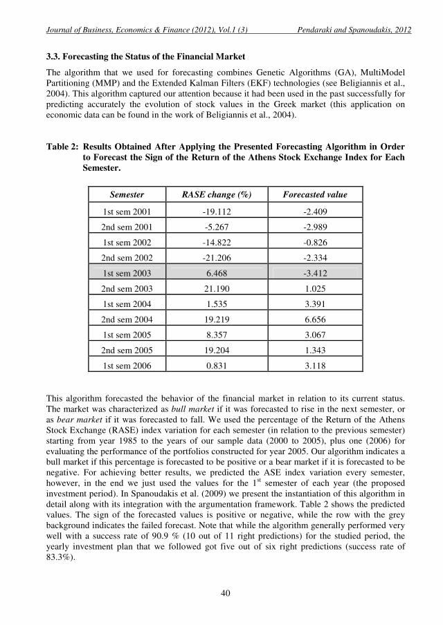
Table 2: Results Obtained After Applying the Presented Forecasting Algorithm in Order
to Forecast the Sign of the Return of the Athens Stock Exchange Index for Each
Semester.
Semester RASE change (%) Forecasted value
1st sem 2001 -19.112 -2.409
2nd sem 2001 -5.267 -2.989
1st sem 2002 -14.822 -0.826
2nd sem 2002 -21.206 -2.334
1st sem 2003 6.468 -3.412
2nd sem 2003 21.190 1.025
1st sem 2004 1.535 3.391
2nd sem 2004 19.219 6.656
1st sem 2005 8.357 3.067
2nd sem 2005 19.204 1.343
1st sem 2006 0.831 3.118
This algorithm forecasted the behavior of the financial market in relation to its current status.
The market was characterized as bull market if it was forecasted to rise in the next semester, or
as bear market if it was forecasted to fall. We used the percentage of the Return of the Athens
Stock Exchange (RASE) index variation for each semester (in relation to the previous semester)
starting from year 1985 to the years of our sample data (2000 to 2005), plus one (2006) for
evaluating the performance of the portfolios constructed for year 2005. Our algorithm indicates a
bull market if this percentage is forecasted to be positive or a bear market if it is forecasted to be
negative. For achieving better results, we predicted the ASE index variation every semester,
however, in the end we just used the values for the 1st semester of each year (the proposed
investment period). In Spanoudakis et al. (2009) we present the instantiation of this algorithm in
detail along with its integration with the argumentation framework. Table 2 shows the predicted
values. The sign of the forecasted values is positive or negative, while the row with the grey
background indicates the failed forecast. Note that while the algorithm generally performed very
well with a success rate of 90.9 % (10 out of 11 right predictions) for the studied period, the
yearly investment plan that we followed got five out of six right predictions (success rate of
83.3%).

Journal of Business, Economics & Finance (2012), Vol.1 (3) Pendaraki and Spanoudakis, 2012
41
3.4. Portfolio Funds Participation Strategies
Having selected the funds that will compose the investment portfolio, through the reasoning
phase, we had the challenge of choosing the participation percentage of each one of them to the
final portfolio. Therefore, we defined a weight vector ),..,( 21 Nwwww = , where each iw
defines the proportion of the available capital invested in the selected funds. We defined four
different portfolio construction strategies for computing this vector.
In the first portfolio construction strategy (or equal participation strategy) the portion of the
portfolio that is allocated to the ith
selected fund (i=1,…,N, where N is the number of total funds
selected by the reasoning phase) is equal, i.e.:
Nwi /1= .
In the second strategy (or performance-based participation strategy), iw is dependent on the
performance of the ith
fund in the current year:
∑=
=N
j
y
j
y
ii
r
rw
1
0
0
,
wherey0 is the current year and y
ir is the return on investment (RoI) value of the ith
selected
fund for year y.
In the third strategy (or history-based participation strategy), iw is dependent on the years where
the ith
fund had high performance:
∑∑
∑
= =
==
N
j
y
yy
y
j
y
yy
y
i
i
h
h
h
h
w
1
0
0
,
whereyk is the year from which we have historical data andy
ih is defined as:
∈
=otherwise
Hrh
yy
iy
i,0
,1.
In the fourth and final portfolio construction strategy (or history combined with performance-
based participation strategy), iw is defined as follows (a mix of the two previous strategies):

Journal of Business, Economics & Finance (2012), Vol.1 (3) Pendaraki and Spanoudakis, 2012
42
∑∑
∑
= =
==
N
j
y
yy
y
j
y
j
y
yy
y
i
y
i
i
h
h
rh
rh
w
1
0
0
4. THE PORTRAIT TOOL
4.1. Architecture
The PORTRAIT tool is a Java program creating a human-machine interface and managing its
modules, namely (see Figure 1):
• the decision making module, which is a prolog rule base (executed in the SWI-prolog1
environment) using the Gorgias2 argumentation framework,
• the forecasting module, which is a Matlab3 implementation of the forecasting hybrid
system,
• thedata import module, which uses Visual Basic for Applications code in Microsoft
Excel to transform the tabular data that are obtained by web sources to the logic format
needed by Prolog.
Figure 1: The Portrait Tool Architecture.
1SWI-Prolog offers a comprehensive Free Software Prolog environment, http://www.swi-
prolog.org 2Gorgias is an open source general argumentation framework that combines the ideas of
preference reasoning and abduction, http://www.cs.ucy.ac.cy/~nkd/gorgias/ 3MATLAB
® is a high-level language and interactive environment for performing
computationally intensive tasks, http://www.mathworks.com/products/matlab

Journal of Business, Economics & Finance (2012), Vol.1 (3) Pendaraki and Spanoudakis, 2012
43
The application connects to the SWI-Prolog module using the provided Java interface (JPL) that
allows for inserting facts to an existing rule-base and running it for reaching goals. The goals can
be captured and returned to the Java program. The forecasting module writes the results of the
algorithm to the Prolog facts base along with the data import module. Thus, after the execution
of the forecasting module the predicate market/1 is determined as bull or bear and inserted in the
Facts.
4.2. Tool Usage
The PORTRAIT user can take the following actions:
1. Select the investment period (i.e. the year of the investment)
2. The investor can select his profile that can be:
a. Either aggressive or moderate in attitude
b. Possibly seeking a high performance per unit of risk
c. He might want to not use the forecasting algorithm results at all or dictate his
own forecast according to his private information for the financial market (to
characterize the market in the following year as bull or bear)
3. The investor chooses the portfolio construction strategy
4. The tool runs the selected scenario outputting the final portfolio
In Figure 2, a screenshot from the tool usage is presented. The user has just run four different
investment scenarios for year 2005.
Journal of Business, Economics & Finance (2012), Vol.1 (3) Pendaraki and Spanoudakis, 2012
44
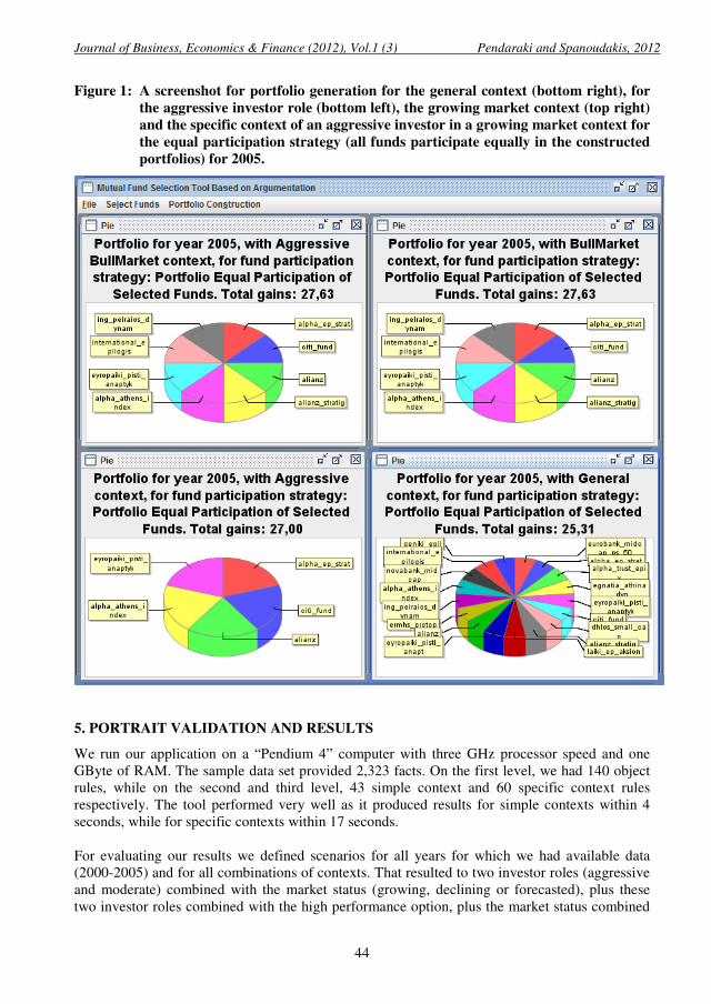
Figure 1: A screenshot for portfolio generation for the general context (bottom right), for
the aggressive investor role (bottom left), the growing market context (top right)
and the specific context of an aggressive investor in a growing market context for
the equal participation strategy (all funds participate equally in the constructed
portfolios) for 2005.
5. PORTRAIT VALIDATION AND RESULTS
We run our application on a “Pendium 4” computer with three GHz processor speed and one
GByte of RAM. The sample data set provided 2,323 facts. On the first level, we had 140 object
rules, while on the second and third level, 43 simple context and 60 specific context rules
respectively. The tool performed very well as it produced results for simple contexts within 4
seconds, while for specific contexts within 17 seconds.
For evaluating our results we defined scenarios for all years for which we had available data
(2000-2005) and for all combinations of contexts. That resulted to two investor roles (aggressive
and moderate) combined with the market status (growing, declining or forecasted), plus these
two investor roles combined with the high performance option, plus the market status combined

Journal of Business, Economics & Finance (2012), Vol.1 (3) Pendaraki and Spanoudakis, 2012
45
with the high performance option, all together eleven different scenarios run for six years each,
plus the simple contexts, roles and preference. Each one of the examined scenarios refers to
different investment choices and leads to the selection of different number and combinations of
MFs.
The evaluation of the proposed methodological framework and the obtained portfolios (in year t)
is performed through their comparison to the return of the Athens Stock Exchange General Index
(ASE-GI) and the average performance of the examined MFs (in year t+1). In Table 3, the
reader can inspect the average return on investment (RoI), i.e. the performance of the constructed
portfolios, for the six years for all different contexts and for all four different portfolio
construction strategies, while in the last two rows of the table the average returns of the ASE-GI
and of the examined MFs are presented. This table shows the added value of our approach.
While there are roles and/or contexts that are more successful than others they are all better than
the average performance of the considered MFs and most of them (14 out of 18) beat the general
market index. This validates our approach as it shows that while we allow the investor to insert
information relevant to his profile we can also offer high returns, always better than the average
performance of the mutual funds of the Greek market. Moreover, we gain information on the
Greek market.
Firstly, an investor that uses the bull market rules gains a better average return than by using our
forecasting algorithm. Among the six examined years three were positive for the market index
(growing or bull market) and three were negative (declining or bear market). An aggressive
investor is also quite successful regardless of whether the market rises or not.
Three of the six cases where the constructed portfolios did not beat the market index are
scenarios where the moderate context is involved either in simple context or specific context (3d,
12th
and 14th
scenario). This is maybe due to the fact that in these contexts we have an investor
who wishes to earn more without taking any amount of risk in the examined period where the
market is characterized by significant variability. The simple general context also performs less
than the Athens GI and shows that the successful MFs of one year are not generally successful
the next year, however, they provide better performance than the average of all MFs. The
remaining two cases where the portfolio returns were less than the market index involve
scenarios with the high performance role (i.e. the 17th
and the 18th
). As we have already
mentioned, the high performance context characterizes mutual funds with high reward-to-
variability ratio and high reward-to-volatility ratio, i.e. the ones with the best managed securities.
In this case the performance of a mutual fund manager is the one that is taken into account.
Again, the variability of the market in the examined period makes it very difficult to implement
successful investment strategies.
Additionally, there are findings that cannot be depicted in such a concentrative table as Table 3.
The most important one is related with the use of argumentation and is that in some specific
contexts the results are more satisfying than the results obtained by simple contexts while in
others there is little or no difference. This means that using effective strategies in the third
preference rules layer the decision maker can optimize the combined contexts. Specifically, in
Table 4the reader can see the return of investment for each year for the aggressive role, the high
performance context and the specific context of their combination when the portfolio has been
constructed with the third strategy. Note that the average RoI of the combination is higher than
that of the individual contexts. Moreover, note that for the year 2005 (first column) the RoI of
the combination of the scenarios is higher than both scenarios. This shows that by successfully

Journal of Business, Economics & Finance (2012), Vol.1 (3) Pendaraki and Spanoudakis, 2012
46
selecting the priority rules at the third level we add knowledge to the knowledge base thus we are
able to provide better results. The pies in Figure 2 agree to this finding as when the growing
market context and the aggressive investor role for year 2005 are merged, the best RoI choice is
selected by the priority rules, thus the specific context has the return of the growing market
context (i.e. 27.63%).
In Table 5, we present the return on investment for different diversities of funds participation in
the constructed portfolios. Each one of the examined contexts refers to different investment
choices and leads to the selection of different number and combinations of MFs. From a total of
59 constructed portfolios, the MFs which composed them ranged between three and 19. Looking
at the results of this table, it is obvious that the more diversified a portfolio is, the higher average
return on investment it has.
We applied the four strategies detailed in §3.4 to all portfolio construction scenarios for the years
2001 to 2005. Each of these strategies can be combined with each investment context. The
investor can choose the strategy that best fits his needs. Our results show that the success of the
portfolio is mainly dependent on the selected context. The best average performance, 7.03%, is
gained by the first portfolio construction strategy, i.e. the equal participation of all funds in the
final portfolio, while according to the second, third and fourth investment strategies, the average
gains for all constructed portfolios and all contexts are 6.83%, 6.62% and 6.42% respectively.
Thus, our research shows that the success of an asset does not in general depend on its past
performance. Figure 3 illustrates these results.

Journal of Business, Economics & Finance (2012), Vol.1 (3) Pendaraki and Spanoudakis, 2012
47
Table 3: Average Return on Investment for Six Years
Scenario
ID Context type Context RoI
1 Simple context General 6.43
2 Role Aggressive 7.22
3 Role Moderate 5.85
4 Preference High performance 6.85
5 Simple context Growing market 7.18
6 Simple context Declining market 7.03
7 Simple context Forecasted Market 6.84
8 Specific
context Aggressive role in a Growing Market 7.18
9 Specific
context Aggressive role in a Declining Market context 6.87
10 Specific
context Aggressive role in a forecasted Market context 7.07
11 Specific
context Aggressive role and High Performance seeking role 7.11
12 Specific
context Moderate role in a Growing Market 5.85
13 Specific
context Moderate role in a Declining Market 6.80
14 Specific
context Moderate role in a forecasted Market context 5.44
15 Specific
context Moderate role and High Performance seeking role 6.85
16 Specific
context
Growing Market context with a High Performance seeking
role 6.85
17 Specific
context
Declining Market context with a High Performance
seeking role 6.42
18 Specific
context
Forecasted Market context with a High Performance
seeking role 6.42
ASE-GI - - 6.75
Avg MFs - - 4.80
Table 4: The Roifor all Years for the third Strategy for the Specific Scenarios
Year 2005 2004 2003 2002 2001 2000 Avg
Co
nte
xt Aggressive 19.53 27.56 9.93 29.63 -25.33 -21.31 6.67
High Perf. 20.73 28.33 14.12 23.79 -27.47 -21.19 6.39
Aggressive - High Perf. 21.77 27.21 9.54 29.63 -25.33 -21.31 6.92

Journal of Business, Economics & Finance (2012), Vol.1 (3) Pendaraki and Spanoudakis, 2012
48
Table 5: Average Return on Investment for Different Funds Participation Number in the
Constructed Portfolios. The Last Column Shows the Percentage of the
Constructed Portfolios that Belongs to Each Category.
Number of Funds
participating in portfolio Average RoI %No
3-8 5.22 32.20
9-15 7.06 49.15
16-19 10.34 18.64
Figure 2: Average Performance of the Portfolio Construction Strategies Compared with
RASE and Average Performance of all MFS for Each Year.
6. CONCLUSIONS AND FUTURE PERSPECTIVES
This paper presented a methodology for the MF portfolio generation problem. The main result of
our work is the ability of a decision maker (fund manager) to construct multi-portfolios of MFs
under different, possibly conflicting contexts that can achieve higher returns than the ones
achieved using simple knowledge. The proposed framework can embody in a direct way the
various decision policies and knowledge (Kakas and Moraitis, 2003) and is used for the first time
for this type of application.
The empirical results of our study showed that argumentation is well suited for this type of
applications and showed our hypothesis “that the proposed methodological framework for the
resolution of the presented financial problem” to be true. Thus, with our approach we answered
to two questions: (1) which MFs are the most suitable to invest in, and (2) what portion of the
available capital should be invested in each of these funds. The proposed methodology gives the
opportunity to a decision maker (fund manager) to construct multi-portfolios of MFs in period t,

Journal of Business, Economics & Finance (2012), Vol.1 (3) Pendaraki and Spanoudakis, 2012
49
that have the ability to achieve higher returns than the ones achieved from the ASE-GI in the
next period, t+1.
The PORTRAIT tool has been validated using the data set described in this paper and is
available for demonstration at the Applied Mathematics and Computers Laboratory (AMCL) of
the Technical University of Crete, Greece. It is intended for use by banks, investment institutions
and consultants, and the public sector.
Our future work is related to the optimization of the strategies so that all combinations add value
to the decision maker. Moreover, it would be of interest to integrate this methodology with
trading approaches, so that one could monitor his portfolio in real time and perform changes to
the portfolio composition instantly as new information becomes available. Thus, it would be of a
great interest to make our tool web-based incorporating: (a) on-line questionnaire for
determining the investor role properties, (b) on-line feed from capital market, and (c) capability
to determine when to update the portfolio (buy or sell) – possibly with a new knowledge base.
References
L.Amgoud and S.Kaci, An argumentation framework for merging conflicting knowledge bases:
The prioritized case, Lecture Notes in Computer Science (LNCS), 3571,(2005), Springer-Verlag,
527–538.
G.N.Beligiannis, L.V .Skarlas and S.D.Likothanassis, A Generic Applied Evolutionary Hybrid
Technique for Adaptive System Modeling and Information Mining, IEEE Signal Processing
Magazine, special issue in Signal Processing for Mining Information,21(3),(2004), 28-38.
S.J. Brown andW.N. Goetzmann, Performance persistence,Journal of Finance,50 (1995), 679-
698.
J.B. DeLong, A. Shleifer, L.H. Summers and R.J.Waldmann, Noise Trader Risk in Financial
Markets,Journal of Political Economy, 98(4), (1990), 703-738.
E.J. Elton and M.J. Gruber, Modern Portfolio Theory and Investment Analysis, Fifth edition,
John Wiley & Sons, New York,(1995).
E.J. Elton, M.J. Gruber, S. Das and M.Hlavka, Efficiency with costly information: A
reinterpretation of evidence from managed portfolios,The Review of Financial Studies,6(1),
(1993), 1-22.
J.G. Gallo and P.E. Swanson, Comparative measures of performance for U.S.-based international
equity mutual funds,Journal of Banking and Finance,20,(1996), 1635-1650.
B.P. Gladish, D.F. Jones, M. Tamiz and A.B. Terol, An interactive three-stage model for mutual
funds portfolio selection,OMEGA35, (2007), 75-88.
M.J. Gruber, Another puzzle: The growth in actively managed mutual funds,Journal of
Finance,51, (1996), 783-810.
D. Hendricks, J. Patel and R.Zeckhauser, Hot hands in mutual funds: Short-Run Persistence of
relative performance, 1974-1988,Journal of Finance,48(1), (1993), 93-130.
R.A. Ippolito, Efficiency with costly information: A study of mutual fund performance, 1965-
1984,Quarterly Journal of Economics, 104,(1989), 1-23.
Journal of Business, Economics & Finance (2012), Vol.1 (3) Pendaraki and Spanoudakis, 2012
50
C.M.Jensen, Risk, the pricing of capital assets, and evaluations of investment portfolio,Journal of
Business, 42,(1969), 67-247.
R.N. Kahn and A. Rudd, Does historical performance predict future performance. Financial
Analysts Journal, (November-December), (1995), 43-53.
A. Kakas and P. Moraïtis Argumentation based decision making for autonomous agents,
Proceedings of the second International Joint Conference on Autonomous Agents and Multi-
Agent Systems (AAMAS’03), Australia, July 14-18, (2003), 883-890.
H. Markowitz, Portfolio Selection: Efficient Diversification of Investments, John Wiley, New
York (1959).
J. Mossin, Optimal Multiperiod Portfolio Policies,Journal of Business,41, (1969), 215-229.
A. Redman, N. Gullett and H. Manakyan, The performance of global and international mutual
funds, Journal of Financial and Strategic Decisions, 13(1), (2000), 75-85.
S. Ross,The Arbitrage Theory of Capital Asset Pricing,Journal of Economic Theory,6
(December), (1976), 341-360.
W.F. Sharpe, Capital asset prices: A theory of market equilibrium under conditions of
risk,Journal of Finance,19, (1964), 425-442.
W.F. Sharpe, Mutual fund performance,Journal of Business,39, (1966), 119-138.
O. Shy, R. Stenbacka, Market structure and diversification of mutual funds,Journal of Financial
Markets,6, (2003), 607-624.
N. Spanoudakis, K. Pendaraki andG. Beligiannis, Portfolio Construction Using Argumentation
and Hybrid Evolutionary Forecasting Algorithms,International Journal of Hybrid Intelligent
Systems,6(4), (2009), 231-243.
V. Subramanian, M.S. Hung and M.Y. Hu, An experimental evaluation of neural networks for
classification,Computers and Operations Research, 20(7),(1993), 769-782.
J.L. Treynor, How to rate management of investment funds,Harvard Business Review,43,
(1965), 63-75.
Appendix A
The Return of the funds is the actual value of return of an investment. The fund’s return in period
t is defined as follows: 11 /)( −−−+= tttpt NAVNAVDISTNAVR , where Rpt is the return of mutual
fund in period t, NAVt is the closing net asset value of the fund on the last trading day of the
period t, NAVt-1 is the closing net asset value of the fund on the last trading day of the period t-1,
and DISTt is the income and capital distributions (dividend of the fund) taken during period t.
The standard deviationσis used to measure the variability of its daily returns, thus representing
the total risk of the fund.The standard deviation of a MF is defined as follows:
∑ −=2)()/1( ptpt RRTσ , where σ is the standard deviation of MF in period t, ptR is the
average return in period t, and T is the number of observation (days) in the period for which the
standard deviation is being calculated.

Journal of Business, Economics & Finance (2012), Vol.1 (3) Pendaraki and Spanoudakis, 2012
51
The beta coefficient (β) is a measure of fund’s risk in relation to the capital market. The beta
coefficient is defined as follows: β = cov (Rpt, RMt) / var (RMt), where cov (Rpt, RMt) is the
covariance of daily return of MF with market portfolio (Athens Stock Exchange), and var (RMt)
is the variance of daily return of market portfolio.
The Sharpe index(Sharpe, 1996) is used to measure the expected return of a fund per unit of risk,
defined by the standard deviation. This measure is defined as the ratio (Rpt- Rft) / σ, where Rft is
the return of the risk free portfolio expressed through the three-month treasury bill.
The Treynor index(Treynor, 1965) is obtained by simply substituting volatility for variability in
the Sharpe index. This measure is defined as the ratio (Rpt- Rft) / β. The evaluation of MFs with
these two indices shows that a MF with higher performance per unit of risk is the best-managed
fund, while a MF with lower performance per unit of risk is the worst managed fund.


