
Air fluidized balls in a background of smaller beads
M. E. Beverland, L. J. Daniels and D. J. Durian
Department of Physics & Astronomy, University of Pennsylvania, Philadelphia,
Pennsylvania 19104-6396, USA
Abstract. We report on quasi-two-dimensional granular systems in which either one or
two large balls is fluidized by an upflow of air in the presence of a background of several
hundred smaller beads. A single large ball is observed to propel ballistically in nearly
circular orbits, in direct contrast to the Brownian behavior of a large ball fluidized in the
absence of this background. Further, the large ball motion satisfies a Langevin equation
with an additional speed-dependent force acting in the direction of motion. This results
in a non-zero average speed of the large ball that is an order of magnitude faster than the
root mean square speed of the background balls. Two large balls fluidized in the absence of
the small-bead background experience a repulsive force depending only on the separation
of the two balls. With the background beads present, by contrast, the ball-ball interaction
becomes velocity-dependent and attractive. The attraction is long-ranged and inconsistent
with a depletion model; instead, it is mediated by local fluctuations in the density of the
background beads which depends on the large balls’ motion.
1. Introduction
A major challenge of modern physics is to understand the behaviour of non-thermal systems
[1, 2], such as granular media [3, 4, 5]. Just as for their thermal counterparts, these
systems can display well-defined statistical distributions that encapsulate their behavior.
For thermal systems, the standard theory of statistical mechanics can be used to predict
all such distributions from equations of motion based on interaction forces plus stochastic
forces set by temperature [6]. For non-thermal systems, by contrast, there is no such general
approach. But in some special cases, experiments have found thermal-like behavior in the
shape of distributions and in the agreement of distinctly defined effective temperatures
[7, 8, 9, 10, 11, 12, 13, 14, 15, 16, 17]. Unfortunately there is no general framework for
determining when such a thermal analogy ought to hold. To make progress, experimentally, it
is sensible to compile further examples of different kinds of driven systems where microscopic
statistical distributions may be measured.
Here we report on measurements of a system consisting of a monolayer of hundreds
of small beads, together with one or two large balls, fluidized in a steady upflow of air.
These beads and balls all roll on a horizontal sieve without slipping and experience in-plane
arX
iv:1
012.
0438
v1 [
cond
-mat
.sof
t] 2
Dec
201
0

forces from collisions with one another and from the air that flows up through them at high
Reynolds number. Previous experiments with this apparatus have shown that a single ball
[13], as well as dense collections of many beads [16], all behave thermally. However, for
two spheres the thermal analogy is progressively broken by increasing the size disparity [15].
Here, for one large ball in a background of small beads, it is therefore unclear in advance
whether or not to expect thermal behavior. Furthermore, for two large balls in a background
of small beads, it is unclear in advance whether to expect the interaction between two large
balls to be repulsive due to turbulence, as in Ref. [15], or to be attractive due to a depletion-
like entropic force mediated by the thermal background of small beads. The latter possibility
of a non-equilibrium depletion force was found in Ref. [18] for a system of large balls in a
background of small beads, all subject to vertical vibration. Our motivation is both to
explore these specific issues, as well as to provide a well documented experimental system
to help motivate and test future statistical theories for non-thermal systems.
Our approach is based on high speed digital video, to track the sphere positions versus
time. We begin with the behavior of the one-ball system in Section 3. The large ball
is observed to propel ballistically through the background medium, creating compressed
and rarefied regions in the background beads. We quantify these local fluctuations in the
background density in Section 3.1. We then characterize the large ball behavior by measuring
statistical distributions, calculating the ball dynamics, and identifying its equation of motion.
We find that the background generates a novel speed-dependent force on the large ball which
accelerates it forward, causing it to move much faster than the small beads. In Section 4, we
analyze the two-ball system and calculate the same time-independent statistical distributions
and dynamics for the two large balls. Lastly, in Section 5, we deduce the interaction between
the two simultaneously-fluidized large balls, which we show to be long-ranged and attractive.
The magnitude and the range are both larger than for a depletion force.
2. Experimental Details
The principal system that we investigate, shown in Fig. 1(a), involves a monolayer of
bidisperse plastic spheres – having radii 0.477 cm and 0.397 cm and masses 0.21 g and 0.165 g,
respectively – fluidized by an upflow of air. This monolayer constitutes the background and
occupies an area fraction of 55% in the absence of larger fluidized balls. This particular
area fraction was chosen so that the background is uniformly distributed across the entire
system. The larger balls fluidized in the presence of this background are ping-pong balls
– radius a = 1.9 cm and mass m = 2.7 g – that have been spray-painted silver to aid in
visualization. Other systems have been analyzed but, except where noted, the diameter ratio
of the large ball to the average diameter of the background is 4.4.
The full system – background beads and one or two large balls – is fluidized by an upflow
of air at 300 cm/s, spatially and temporally homogeneous within ±10 cm/s and 0.5 s, as
2

Figure 1. a) A large sphere, radius a = 1.9 cm and mass 2.7 g, fluidized in the presence of
a bidisperse background of smaller spheres – radii 0.477 cm and 0.397 cm and masses 0.21 g
and 0.165 g, respectively. The diameter ratio of the large ball to the background beads is
4.4. The radius of the system is R = 14.3 cm. The vectors define position ~r, velocity ~v, as
well as the polar angle θ as measured from the horizontal axis. b) A one-minute long trace
of the position of the large ball shown in a). To emphasize the observed circular motion,
the trace is colored red for clockwise motion, blue for counterclockwise.
verified by a hot-wire anemometer. The Reynolds number is 104 such that the motion of the
balls is driven stochastically by turbulence. The airflow is below the terminal free fall speed
of the balls, which ranges from 700-800 cm/s according to mg = 0.43(ρair/2)v22πr2, so that
the balls maintain contact with the sieve and move by rolling without slipping. As such, we
define an effective mass meff = m+ I/r2, where I is the moment of inertia.
The apparatus, fluidization method, and lighting setup are identical to those of Ref. [19].
The apparatus is a rectangular windbox, 1.5×1.5×4 ft.3, positioned upright, with two nearly
cubical chambers separated by a perforated metal sheet. A blower attached to the windbox
base by a flexible cloth sleeve provides vertical airflow perpendicular to a circular brass
testing sieve with mesh size 150 µm and radius 15.3 cm that rests horizontally on top. To
prevent background spheres from getting caught in a small groove at the inner edge of the
sieve, we place a 0.953 cm-diameter norprene tube around its inside edge. Thus, the system
has an actual radius, R = 14.3 cm.
The particles are illuminated from above by six 100 W incandescent bulbs arranged in
a 1-foot diameter ring positioned 3 feet above the sieve. A digital CCD camera placed at
the center of this ring captures the raw video data, typically for 4 hours at a time at 120
frames per second. We threshold these long videos to binary as they save to buffer so that
only the highly-reflective large ball is seen. Post-processing of the video data is accomplished
using LabVIEW, using custom particle-tracking programs. From the center-of-mass position
obtained from the video data, we determine velocity and acceleration by fitting the position
3
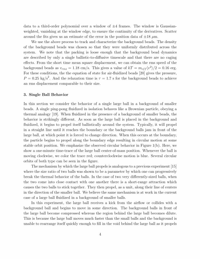
data to a third-order polynomial over a window of ±4 frames. The window is Gaussian-
weighted, vanishing at the window edge, to ensure the continuity of the derivatives. Scatter
around the fits gives us an estimate of the error in the position data of ±18 µm.
We use the above process to track and characterize the background beads. The density
of the background beads was chosen so that they were uniformly distributed across the
system. We note that the packing is loose enough that the background bead dynamics
are described by only a single ballistic-to-diffusive timescale and that there are no caging
effects. From the short time mean square displacement, we can obtain the rms speed of the
background beads as vrms = 1.18 cm/s. This gives a value of kT = meff〈v2〉/2 = 0.16 erg.
For these conditions, the the equation of state for air-fluidized beads [20] gives the pressure,
P = 0.25 kg/s2. And the relaxation time is τ = 1.7 s for the background beads to achieve
an rms displacement comparable to their size.
3. Single Ball Behavior
In this section we consider the behavior of a single large ball in a background of smaller
beads. A single ping-pong fluidized in isolation behaves like a Brownian particle, obeying a
thermal analogy [19]. When fluidized in the presence of a background of smaller beads, the
behavior is strikingly different. As soon as the large ball is placed in the background and
fluidized, it begins to propel itself ballistically around the system. Typically, it will propel
in a straight line until it reaches the boundary or the background balls jam in front of the
large ball, at which point it is forced to change direction. When this occurs at the boundary,
the particle begins to propel along the boundary edge resulting in circular motion at some
stable orbit position. We emphasize the observed circular behavior in Figure 1(b). Here, we
show a one-minute time-trace of the large ball center-of-mass position. Whenever the ball is
moving clockwise, we color the trace red; counterclockwise motion is blue. Several circular
orbits of both type can be seen in the figure.
The mechanism by which the large ball propels is analogous to a previous experiment [15]
where the size ratio of two balls was shown to be a parameter by which one can progressively
break the thermal behavior of the balls. In the case of two very differently-sized balls, when
the two come into close contact with one another there is a short-range attraction which
causes the two balls to stick together. They then propel, as a unit, along their line of centers
in the direction of the smaller ball. We believe the same mechanism is at work in the current
case of a large ball fluidized in a background of smaller balls.
In this experiment, the large ball receives a kick from the airflow or collides with a
background ball and begins to move in some direction. The background balls in front of
the large ball become compressed whereas the region behind the large ball becomes dilute.
This is because the large ball moves much faster than the small balls and the background is
unable to rearrange itself quickly enough to fill in the void behind the large ball as it propels
4

through the system. The dilute wake behind the ball is easily visible in Fig. 1(a). The
compressed region in front of the large ball behaves just like the smaller ball in the earlier
two-ball experiment. The large ball moves in the direction of this compressed region and
gains speed. This also suggests that the local fluctuations in the background density will be
dependent on the speed of the large ball.
To quantify these observations, we begin by analyzing the effect of the large ball
on the distribution of background balls; we then calculate time-independent probability
distributions and the dynamics of the large ball.
3.1. Background Beads
Rather than track the individual background beads, we quantify the local density fluctuations
graphically. We first track the large ball position and then obtain its velocity in each frame.
Then, each frame in the video was rotated and had its origin shifted such that the large ball
was centered and moving to the right along the horizontal axis. Since we have suggested
that the local density is dependent on the large ball speed, we bin these processed images
according to the speed of the large ball and then average over all images within each speed
bin. The results, for three different ranges of large ball speeds, are shown in Fig. 2. The
images have been color-coded by linearly interpolating the grayscale values between 0% area
fraction, shown as black, and jammed particles at 84%, shown as white.
Figure 2. Time-averaged density of the background for three different ranges of the large
ball speed, as specified below each image. The large ball (outlined in white), radius 1.9 cm,
is always moving horizontally to the right. The density scale linearly interpolates between
0% area fraction (black) and a jammed region at 84% (white).
The effect is very dramatic. In the left image, the large ball – outlined by a white circle
– is moving very slowly and the compressed and dilute regions are relatively small. As we
increase speed from left to right, we observe that both the compressed region in front of the
ball and the dilute wake behind the ball become larger. The slight asymmetry in the image
5

is due to the ball circulating in the counterclockwise direction more often than clockwise for
the video analyzed.
To quantify the difference in density between the compressed and rarefied regions, we
obtain the average packing fraction within hemispherical annular areas both in front of,
φahead, and behind, φbehind, the large ball. We then plot the difference between these packing
fractions as a function of the large ball speed, as shown in Fig. 3. The results show that the
extent of the compression and rarefaction, and thus interaction of the large ball with the
background, depends on the speed v of the large ball. The effect vanishes in the limit of zero
speed, and saturates at φahead − φbehind ≈ 0.6 for v > 10 cm/s.
Figure 3. The average difference in packing fraction of the background beads on opposites
sides of a large fluidized ball as a function of its speed. The beads are compressed in front
and rarified in back, as seen in Fig. 2.
3.2. Statics
Because our system reaches a steady state very quickly, the simplest way in which to
characterize it is by compiling statistics of time-independent quantities. Intuitively, we
thought that the presence of the turbulent background would serve to overwhelm repulsive
interactions of the large ball with the bounding walls. In other words, the large ball would
move in a random walk, sampling all of the system space equally. In this case, the radial
probability distribution P (r)/r – where we divide by r to account for the fact that there
are more points in phase space further from the origin – would be constant from the origin
r = 0 to the effective reduced radius of the system R′ = R − a = 12.4 cm, at which point
the distribution would discontinuously vanish.
The observed P (r)/r for our system is shown in Fig. 4(a). In no region is the distribution
constant, suggesting that the background may actually enhance the interaction with the
boundary. There is a large peak at an intermediate radius as the large ball begins to detect
6
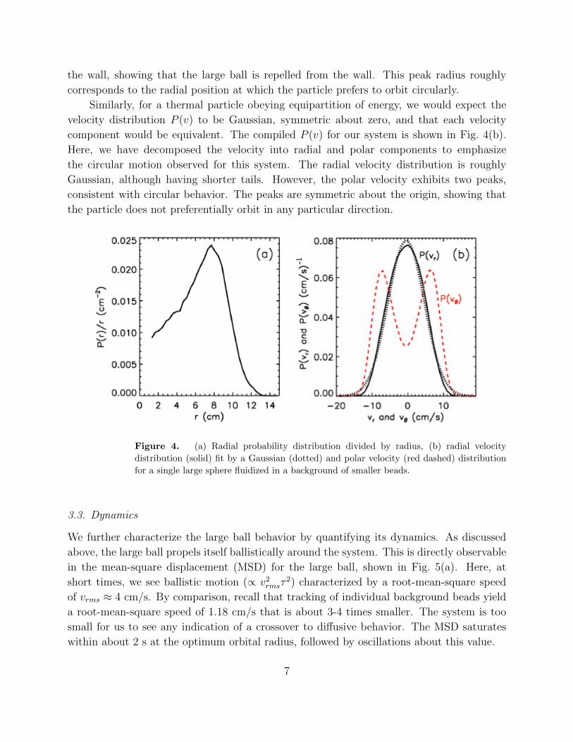
the wall, showing that the large ball is repelled from the wall. This peak radius roughly
corresponds to the radial position at which the particle prefers to orbit circularly.
Similarly, for a thermal particle obeying equipartition of energy, we would expect the
velocity distribution P (v) to be Gaussian, symmetric about zero, and that each velocity
component would be equivalent. The compiled P (v) for our system is shown in Fig. 4(b).
Here, we have decomposed the velocity into radial and polar components to emphasize
the circular motion observed for this system. The radial velocity distribution is roughly
Gaussian, although having shorter tails. However, the polar velocity exhibits two peaks,
consistent with circular behavior. The peaks are symmetric about the origin, showing that
the particle does not preferentially orbit in any particular direction.
Figure 4. (a) Radial probability distribution divided by radius, (b) radial velocity
distribution (solid) fit by a Gaussian (dotted) and polar velocity (red dashed) distribution
for a single large sphere fluidized in a background of smaller beads.
3.3. Dynamics
We further characterize the large ball behavior by quantifying its dynamics. As discussed
above, the large ball propels itself ballistically around the system. This is directly observable
in the mean-square displacement (MSD) for the large ball, shown in Fig. 5(a). Here, at
short times, we see ballistic motion (∝ v2rmsτ
2) characterized by a root-mean-square speed
of vrms ≈ 4 cm/s. By comparison, recall that tracking of individual background beads yield
a root-mean-square speed of 1.18 cm/s that is about 3-4 times smaller. The system is too
small for us to see any indication of a crossover to diffusive behavior. The MSD saturates
within about 2 s at the optimum orbital radius, followed by oscillations about this value.
7

To get a sense of the characteristic timescales in our system, we consider the velocity
and acceleration autocorrelation functions as shown in Figs. 5(b) and (c). The velocity
autocorrelation has a long plateau that rolls off after approximately 1 s and then oscillates
as the function decays to zero. This timescale corresponds roughly to the relaxation time
of the large ball arms/vrms ≈ 0.95 s. The strong oscillations are indicative of the circular
motion exhibited by the ball. The acceleration autocorrelation decorrelates much more
quickly than the velocity does, having one small oscillation at 0.08 s, before decaying to zero
at approximately 0.3 s. This separation of timescales is further emphasized by including an
overlay of the mean square acceleration change on the mean square displacement, Fig. 5(a).
Figure 5. (a) Mean square displacement (solid) and mean square acceleration fluctuations
(red dashed), (b) velocity autocorrelation, and (c) acceleration autocorrelation for a single
large sphere fluidized in a background of smaller beads. The effective radius of the system
is the difference R′ = R− a between the system and the large ball radii.
8
3.4. Equation of Motion
In this section, we analyze the large ball motion in terms of a model of the forces acting
on a single large ball fluidized in the presence of a background of smaller beads. A simple
conceivable equation of motion for the large ball is
meff~a = C(r)r̂ +D(v)v̂ + ~ζ(t), (1)
where the forces D(v) and C(r) are functions of the large ball’s speed and radial position,
and ~ζ(t) is a stochastic force satisfying 〈~ζ(t)〉 = 0. The position dependent force C(r)r̂ must
be circularly symmetric since the system has circular symmetry. The velocity dependent
force must include a drag term for the interaction of the large ball with the mesh substrate,
which we will assume to be linear since the velocity decays more slowly than the acceleration.
As we saw in Section 3.1, the interaction of the large ball with the background is also speed-
dependent. Thus, we write D(v)v̂ = −γ~v + β(v)v̂ where −γ~v is the drag term and β(v)v̂ is
the force caused by the background which, for simplicity, we assume to be in the direction
of the large ball velocity v̂.
We will now examine each term of the equation using a dynamical approach. We can
isolate the central force by taking the cross product of (1) with v̂. Rearranging:
C(r)−
[~ζ × v̂r̂ × v̂
]=
(~a× v̂r̂ × v̂
)meff (2)
Similarly, we can isolate the speed-dependent force by taking the cross product of (1) with
r̂, giving:
D(v)−
[~ζ × r̂v̂ × r̂
]=
(~a× r̂v̂ × r̂
)meff (3)
If we assume the stochastic force is independent of position and velocity, the time
average of the square brackets in both (2) and (3) must be zero. Thus, we can readily obtain
C(r), as shown in Fig. 6(a). We see that there is essentially zero force at small radii. At
increasing r, as the ball approaches the bounding walls, the force becomes repulsive. The
solid line in the figure is a fit to C(r) ∝ r3/(r − R′)0.65. This is in contrast to the linear
dependence of this term observed for a large sphere fluidized in an empty sieve [13, 19]. As
a further comparison, the dashed curve is the radial force obtained if we had approximated
the system as thermal and calculated the radial force using the data for P (r), according
to C(r) = − ddrkTeff log(−P (r)/r). The discrepancy between the two methods for deducing
C(r) shows that the system is not behaving thermally.
We can also readily obtain D(v), as shown in Fig. 6(b). For speeds between 0 cm/s and
roughly 10 cm/s, the speed-dependent force is positive, causing the large ball to speed up.
For speeds larger than about 10 cm/s, the force is negative thus slowing the particle. This
is consistent with our earlier observations of the compression/rarefaction that accompanies
9
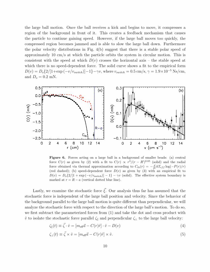
the large ball motion. Once the ball receives a kick and begins to move, it compresses a
region of the background in front of it. This creates a feedback mechanism that causes
the particle to continue gaining speed. However, if the large ball moves too quickly, the
compressed region becomes jammed and is able to slow the large ball down. Furthermore
the polar velocity distributions in Fig. 4(b) suggest that there is a stable polar speed of
approximately 10 cm/s at which the particle orbits the system in circular motion. This is
consistent with the speed at which D(v) crosses the horizontal axis – the stable speed at
which there is no speed-dependent force. The solid curve shows a fit to the empirical form
D(v) = Do{2/[1+exp (−v/vswitch)]−1}−γv, where vswitch = 0.5 cm/s, γ = 1.9×10⁻⁵ Ns/cm,
and Do = 0.2 mN.
Figure 6. Forces acting on a large ball in a background of smaller beads: (a) central
force C(r) as given by (2) with a fit to C(r) ∝ r3/(r − R′)0.65 (solid) and the radial
force obtained via thermal approximation according to Cth(r) = − ddrkTeff log(−P (r)/r)
(red dashed); (b) speed-dependent force D(v) as given by (3) with an empirical fit to
D(v) = Do{2/[1 + exp (−v/vswitch)] − 1} − γv (solid). The effective system boundary is
marked at r = R− a (vertical dotted blue line).
Lastly, we examine the stochastic force ~ξ. Our analysis thus far has assumed that the
stochastic force is independent of the large ball position and velocity. Since the behavior of
the background parallel to the large ball motion is quite different than perpendicular, we will
analyze the stochastic force with respect to the direction of the large ball’s motion. To do so,
we first subtract the parameterized forces from (1) and take the dot and cross product with
v̂ to isolate the stochastic force parallel ζ‖ and perpendicular ζ⊥ to the large ball velocity:
ζ‖(t) ≡ ~ζ · v̂ = [meff~a− C(r)r̂] · v̂ −D(v) (4)
ζ⊥(t) ≡ ~ζ × v̂ = [meff~a− C(r)r̂]× v̂. (5)
10

Since the speed directly enters these equations, we show the stochastic force probability
functions in Fig. 7(a) at the particular speed v = 4.5 cm/s. P (ζ⊥), shown as the solid
curve, is nearly Gaussian. By contrast, the distribution of the parallel stochastic force
is significantly skewed, having much larger probability to provide a kick in the direction of
motion. This shows that our assumption that the stochastic force is independent of the speed
was incorrect. The shape of these distributions does not significantly change depending on
the magnitude of the large ball speed. This is verified in Fig. 7(b) where we plot the standard
deviations σ of the probability distributions P (ζ‖(t)) and P (ζ⊥(t)) as a function of the large
ball speed. Both distributions remain roughly the same width until 8 cm/s, at which point
the distributions narrow. Interestingly, this directional dependence of the stochastic force has
been seen before in the behavior of fluidized rods [21]. In that experiment, it was observed
that the rods self-propel much like the large ball is observed to do in this experiment.
Figure 7. (a) Probability distribution of the stochastic force parallel to (dashed) and
perpendicular to (solid) the large ball velocity, for v = 4.5 cm/s. The dotted curve is a
Gaussian fit to P (ζ⊥). (b) Standard deviation of the stochastic force distributions as a
function of large ball speed.
4. Two Balls Behavior
Having documented the behaviour of a single large ball in a background of smaller balls,
we add a second large ball to the system. When fluidized in an empty sieve, the force
between two balls is characterized by hardcore repulsion and a persistent repulsive force over
all separation distances [19]. With the inclusion of background beads, we might expect a
short-range depletion interaction that would attract the two balls together as well as longer-
range forces mediated by the background. When we place the two large balls in the system,
they both propel ballistically and orbit about the system. Often, the two balls will become
trapped in one another’s wake and travel as a pair. However, they are rarely observed to
11
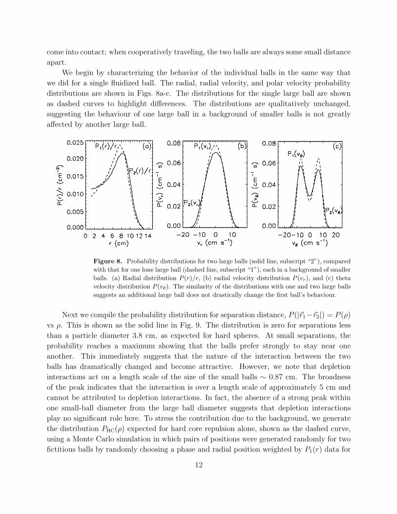
come into contact; when cooperatively traveling, the two balls are always some small distance
apart.
We begin by characterizing the behavior of the individual balls in the same way that
we did for a single fluidized ball. The radial, radial velocity, and polar velocity probability
distributions are shown in Figs. 8a-c. The distributions for the single large ball are shown
as dashed curves to highlight differences. The distributions are qualitatively unchanged,
suggesting the behaviour of one large ball in a background of smaller balls is not greatly
affected by another large ball.
Figure 8. Probability distributions for two large balls (solid line, subscript “2”), compared
with that for one lone large ball (dashed line, subscript “1”), each in a background of smaller
balls. (a) Radial distribution P (r)/r, (b) radial velocity distribution P (vr), and (c) theta
velocity distribution P (vθ). The similarity of the distributions with one and two large balls
suggests an additional large ball does not drastically change the first ball’s behaviour.
Next we compile the probability distribution for separation distance, P (|~r1−~r2|) = P (ρ)
vs ρ. This is shown as the solid line in Fig. 9. The distribution is zero for separations less
than a particle diameter 3.8 cm, as expected for hard spheres. At small separations, the
probability reaches a maximum showing that the balls prefer strongly to stay near one
another. This immediately suggests that the nature of the interaction between the two
balls has dramatically changed and become attractive. However, we note that depletion
interactions act on a length scale of the size of the small balls ∼ 0.87 cm. The broadness
of the peak indicates that the interaction is over a length scale of approximately 5 cm and
cannot be attributed to depletion interactions. In fact, the absence of a strong peak within
one small-ball diameter from the large ball diameter suggests that depletion interactions
play no significant role here. To stress the contribution due to the background, we generate
the distribution PHC(ρ) expected for hard core repulsion alone, shown as the dashed curve,
using a Monte Carlo simulation in which pairs of positions were generated randomly for two
fictitious balls by randomly choosing a phase and radial position weighted by P1(r) data for
12

each. As such, any difference between our data and the simulation is due to interactions either
mediated by the background beads or by the airflow, which is know to be repulsive [19]. The
comparison shows an enhancement of the distribution at close separation, which suggests an
effective attraction between the large balls mediated by the background beads. We further
emphasized that this attractive force is mediated by the background by anchoring one of the
large balls to be stationary while the other large ball freely moves about the system. The
resulting separation probability distribution is identical to the one-ball radial probability
distribution P1(r). Therefore, the attractive force between two free balls is dependent on
their motion through the background and presumably linked to fluctuations in the local
density.
Figure 9. Separation distribution P (ρ) for the separation ρ between two large balls
in a background of smaller balls (solid) and simulation results PHC(ρ) (dashed) for balls
interacting only via hard core repulsion.
5. Ball-Ball Interaction
In this section we seek to quantify the interaction force between two balls in a background
of smaller beads. We assume the same equation of motion as for one large ball, but add
interaction forces:
meff~a1 = C(r1)r̂1 +D(v1)v̂1 + ~ζ1(t) + ~F1 2 (6)
meff~a2 = C(r2)r̂2 +D(v2)v̂2 + ~ζ2(t) + ~F2 1 (7)
Assuming ~F1 2 depends only on ρ, we define an interaction potential Vs(ρ) according to
~F1 2(ρ) = [−dVs(ρ)/dρ]ρ̂1 2 where ρ̂1 2 = (~r1 − ~r2)/|~r1 − ~r2| (8)
First, we want to determine the interaction potential Vs(ρ) from our data. We can infer this
from the separation distribution P (ρ) if we assume the system behaves sufficiently thermally
such that
P (~r1, ~r2) ∝ exp {−[Vc(r1) + Vc(r2) + Vs(ρ)]/Teff} (9)
13

where the central potential for one-large-ball is given by Vc(r) = −Teff ln(P1(r)/r).
Rearranging (9) and integrating over remaining variables, Vs(ρ) can be obtained from the
measured P (ρ):
Vs(ρ) = −Teff ln[P (ρ)/g(ρ)] + const. (10)
where
g(ρ) = ρ
∫ R−a
0
dr1
∫ 2π
0
dϕ r1 exp
[−(Vc(r1) + Vc(r2))
Teff
]. (11)
The resulting interaction potential is shown as the points in Fig. 10. As expected due to
hard-core repulsion, the potential diverges at one ball diameter. The data has been fit to
the empirical form V fits (ρ) = Vα[(ρ− 2a)/a]α + V0 exp[−(ρ− 2a)/λ].
It is straightforward to show that the data is inconsistent with a depletion attraction.
A depletion interaction between large balls is expected when they are sufficiently close that
small balls cannot access the region between them. The background beads impart a constant
pressure p on all accessible surfaces. This pressure p can be estimated by assuming that the
background beads obey a reduced-volume ideal gas equation of state p = NbTb/Areducedwhere Tb = mb,eff〈v2
b〉 and the reduced area Areduced is the area available to the balls’ centers,
minus the minimum area they could occupy. By integrating over the exposed circumference
of one of the large balls, we can derive the depletion force Fdep(ρ)ρ̂1 2 on ball 1 due to ball
2. This force will be non-zero and finite only for the region 2a < ρ < 2(a + b), where a is
the large ball radius and b is the average background bead radius. In this region, the force
is given as Fdep(ρ) = −2ap√
1− [ρ/(2a+ 2b)]2. Then, we are able to obtain the interaction
potential by integration:
Vdep(ρ) = −2ap
ρ2√
1−[
ρ
2(a+ b)
]2
+ (a+ b) sin−1
[ρ
2(a+ b)
] . (12)
This expression has been plotted alongside our data as the dashed curve in Fig. 10, multiplied
by a factor of 50. Both the range and strength of a depletion attraction are much smaller
than that obtained from the data.
Just as the force on a single ball is speed-dependent, it is likely that the ball-ball
interaction is also dependent on how the balls are moving relative to one another. To
examine this, we first separated the video data into three scenarios of large ball motion:
(i) (→→): moving in same direction [i.e. ~v1 · ~v2 > 0]
(ii) (←→): moving apart [i.e. ~v1 · ~v2 < 0 and dρ/dt > 0]
(iii) (→←): moving closer together [i.e. ~v1 · ~v2 < 0 and dρ/dt < 0]
We then repeat the above analysis to determine the interaction potential for different types
of relative motion. Our results are shown in Fig. 11. The potentials are significantly different
from each other, which is strong evidence that the interaction force depends on the velocity
14

Figure 10. Interaction potential for two large balls in a background of smaller
beads, calculated from the measured separation distribution P (ρ) and assuming thermal
equilibrium. The solid line is a fit to V fits (ρ) = Vα[(ρ− 2a)/a]α + V0 exp[−(ρ− 2a)/λ]. The
dashed line shows the depletion potential Vdep(ρ), multiplied by a factor of 50.
of the large balls as well as their separation. Each scenario displays short range repulsion
with attraction at longer ranges. The strongest attraction occurs when the balls move in the
same direction.
Figure 11. Interaction potentials for two large balls in a background of smaller beads
for different relative motion of the large balls, calculated from the measured separation
distribution P (ρ) and assuming thermal equilibrium: moving in the same direction (→→,
red squares); moving apart (←→, blue triangles); and moving closer together (→←,
green diamonds). The solid curves are best fit lines to the empirical form V fits (ρ) =
Vα[(ρ− 2a)/a]α + V0 exp[−(ρ− 2a)/λ].
15
6. Conclusions
We have characterized the behavior of and forces acting on a large sphere fluidized in a
bidisperse background of smaller beads. The large ball self-propels ballistically through
the medium, strongly perturbing the local density of the background. The presence of the
background not only modifies the central force felt by a fluidized ball moving in an empty
sieve but also mediates a novel speed-dependent force. The speed-dependent force acts to
keep the large ball propelling itself at a stable speed of approximately 10 cm/s. Furthermore,
the stochastic force is directionally-dependent and preferentially kicks the large ball in its
direction of motion. When two large balls are fluidized simultaneously, there is a short-range
repulsion mediated by the airflow, as in Ref. [19] but with a range that is cut off. And there
is a long range attraction mediated by the background beads and dependent on the relative
motion of the two balls. Further, we demonstrated that the attraction is not consistent with
the depletion interaction.
7. Acknowledgments
This work was supported by the NSF through grant DMR-0704147.
References
[1] D. Ruelle, Physics Today 57(5), 48 (2004)
[2] CMMP-2010, Condensed-Matter and Materials Physics: The Science of the World Around Us (The
National Academies Press, Washington, DC, 2007)
[3] R.M. Nedderman, Statics and Kinematics of Granular Materials (Cambridge Univ. Press, NY, 1992)
[4] H.M. Jaeger, S.R. Nagel, R.P. Behringer, Rev. Mod. Phys. 68, 1259 (1996)
[5] J. Duran, Sands, powders, and grains (Springer, NY, 2000)
[6] R. Kubo, M. Toda, N. Hashitsume, Statistical Physics II: Nonequilibrium Statistical Mechanics
(Springer, NY, 2001)
[7] B. Pouligny, R. Malzbender, P. Ryan, N.A. Clark, Phys. Rev. B 42, 988 (1990)
[8] I. Ippolito, C. Annic, J. Lemaitre, L. Oger, D. Bideau, Phys. Rev. E 52, 2072 (1995)
[9] J.S. Olafsen, J.S. Urbach, Phys. Rev. E 60, R2468 (1999)
[10] J. Prentis, Am. J. Phys. 68, 1073 (2000)
[11] G.W. Baxter, J.S. Olafsen, Nature 425, 680 (2003)
[12] G. D’Anna, P. Mayor, A. Barrat, V. Loreto, F. Nori, Nature 424, 909 (2003)
[13] R. Ojha, P.A. Lemieux, P.K. Dixon, A.J. Liu, D. Durian, Nature 427, 521 (2004)
[14] C.M. Song, P. Wang, H.A. Makse, PNAS 102, 2299 (2005)
[15] A.R. Abate, D.J. Durian, Phys. Rev. E 72, 031305 (2005)
[16] A.R. Abate, D.J. Durian, Phys. Rev. Lett. 101, 245701 (2008)
[17] P. Wang, C. Song, C. Briscoe, H.A. Makse, Phys. Rev. E 77, 061309 (2008)
[18] P. Melby, A. Prevost, D.A. Egolf, J.S. Urbach, Phys. Rev. E 76, 051307 (2007)
[19] R.P. Ojha, A.R. Abate, D.J. Durian, Phys. Rev. E 71, 016313 (2005)
[20] L.J. Daniels, T.K. Haxton, N. Xu, A.J. Liu, D.J. Durian. In preparation
[21] L.J. Daniels, Y. Park, T.C. Lubensky, D.J. Durian, Phys. Rev. E 79, 041301 (2009)
16


