
USING REPUTATION BASED TRUST TO OVERCOME MALFUNCTIONS AND MALICIOUS FAILURES IN ELECTRIC POWER PROTECTION
SYSTEMS
DISSERTATION
Jose E. Fadul, Captain, USAF
AFIT/DEE/ENG/11-08
DEPARTMENT OF THE AIR FORCE AIR UNIVERSITY
AIR FORCE INSTITUTE OF TECHNOLOGY
Wright-Patterson Air Force Base, Ohio
DISTRIBUTION STATEMENT A: APPROVED FOR PUBLIC RELEASE; DISTRIBUTION UNLIMITED

The views expressed in this dissertation are those of the author and do not reflect the official policy or position of the United States Air Force, the Department of Defense, or the United States Government. This material is declared a work of the U.S. Government and is not subject to copyright protection in the United States.

AFIT/DEE/ENG/11-08
USING REPUTATION BASED TRUST TO OVERCOME MALFUNCTIONS
AND MALICIOUS FAILURES IN ELECTRIC POWER PROTECTION
SYSTEMS
DISSERTATION
Presented to the Faculty
Department of Electrical and Computer Engineering
Graduate School of Engineering and Management
Air Force Institute of Technology
Air University
Air Education and Training Command
In Partial Fulfillment of the Requirements for the
Degree of Doctor of Philosophy
Jose E. Fadul, B.S.E.E., M.S.E.E.
Captain, USAF
September 2011
DISTRIBUTION STATEMENT A: APPROVED FOR PUBLIC RELEASE; DISTRIBUTION UNLIMITED

AFIT/DEE/ENG/lI-08
USING REPUTATION BASED TRUST TO OVERCOME MALFUNCTIONS AND MALICIOUS FAILURES IN ELECTRIC POWER PROTECTION
SYSTEMS
Jose E. Fadul, B.S.E.E., M.S.E.E. Captain, USAF
Approved:
kenneth M. Hopkinson, PhD (Chairman)
4- · ' ~~
Accepted:
M. U. Thomas, PhD Dean, Graduate School of Engineering and Management
/ ~ :Tv ly:L ) II Date
I 'S A""'-~ 2.CI\, Date

iv
AFIT/DEE/ENG/11-08
Abstract
This dissertation advocates the use of reputation-based trust in conjunction with a
trust management framework based on network flow techniques to form a trust
management toolkit (TMT) for the defense of future Smart Grid enabled electric power
grid from both malicious and non-malicious malfunctions. Increases in energy demand
have prompted the implementation of Smart Grid technologies within the power grid.
Smart Grid technologies enable Internet based communication capabilities within the
power grid, but also increase the grid’s vulnerability to cyber attacks. The benefits of
TMT augmented electric power protection systems include: improved response times,
added resilience to malicious and non-malicious malfunctions, and increased reliability
due to the successful mitigation of detected faults. In one simulated test case, there was a
99% improvement in fault mitigation response time. Additional simulations demonstrated
the TMT’s ability to determine which nodes were compromised and to work around the
faulty devices when responding to transient instabilities. This added resilience prevents
outages and minimizes equipment damage from network based attacks, which also
improves system’s reliability. The benefits of the TMT have been demonstrated using
computer simulations of dynamic power systems in the context of backup protection
systems and special protection systems.

v
AFIT/DEE/ENG/11-08
For my wife and my two daughters

vi
Acknowledgments
I would like to express my sincere appreciation to my research advisor,
Dr. Kenneth M. Hopkinson, and my committee members, Dr. James T. Moore and
Maj Todd R. Andel, for their guidance and support throughout the course of this
dissertation effort. Their insight and experience was certainly appreciated. I would, also,
like to thank my sponsor, Dr. Robert J. Bonneau, from the Air Force Office of Scientific
Research for both the support and latitude provided to me in this endeavor.
I’m also indebted to the many professors who spent their valuable time explaining
the details of computer networks, linear programs, network flows and power systems.
Special thanks go to Col Keith Boyer, Lt Col Stuart Kurkowski, Dr. Nathaniel Davis,
Dr. Rusty Baldwin, Dr. Barry Mullins, Dr. Timothy Lacey, Dr. Gary Lamont,
Mrs. Helen Atkinson, Mrs. Yuvonne Cherne, Mrs. Janice Jones, Mrs. Donna Warren,
Mr. Christopher Sheffield, Mr. Donald Bodle, Mr. David Doak, Mr. Bruce Carter,
Mr. Michael Lovelace, Mr. Charles Powers and Mr. Ryan Harris.
Jose E. Fadul

vii
Table of Contents Page
Abstract .............................................................................................................................. iv
Acknowledgments .............................................................................................................. vi
Table of Contents .............................................................................................................. vii
List of Figures .................................................................................................................... xi
List of Tables ................................................................................................................... xiv
List of Symbols ..................................................................................................................xv
List of Abbreviations ...................................................................................................... xvii
I. Introduction ..................................................................................................................1
1.1 Background .........................................................................................................1
1.2 Strategic Problem Statement ...............................................................................8
1.3 Tactical Problem Statement .................................................................................9
1.4 Research Focus ..................................................................................................10
1.5 What is Reputation Based Trust ........................................................................11
1.6 Methodology .....................................................................................................12
1.6.1 Spiral 1 Simple Trust Protocol. .............................................................12
1.6.2 Spiral 2 Centralized SCADA TMT for PSCAD. ..................................13
1.6.3 Spiral 3 Distributed SCADA TMT for PSCAD. ...................................15
1.6.4 Spiral 4 Distributed SCADA TMT for PSS/E .......................................16
1.7 How the Remainder of this Document is Organized .........................................17
II. Simple Trust Protocol .................................................................................................18
2.1 Introduction .......................................................................................................18
2.2 Background .......................................................................................................20
2.2.1 What is Trust .........................................................................................20
2.2.2 Why is trust needed? .............................................................................21
2.2.3 Trust Classifications. .............................................................................21
2.3 Related Work .....................................................................................................22
2.3.1 CONFIDANT. .......................................................................................22

viii
Page
2.3.2 EigenTrust. ............................................................................................23
2.4 Simple Trust Protocol ........................................................................................24
2.4.1 Simple Trust Design Considerations. ....................................................24
2.4.2 Simple Trust Assumptions. ...................................................................25
2.4.3 Centralized Simple Trust. ......................................................................26
2.5 Experimental Design .........................................................................................31
2.6 Experimental Results .........................................................................................33
2.7 Summary ...........................................................................................................34
III. SCADA Trust Management System ..........................................................................37
3.1 Introduction .......................................................................................................37
3.2 Background and Related Work .........................................................................39
3.2.1 Background. ..........................................................................................39
3.2.2 Related Work. ........................................................................................42
3.3 SCADA Trust Management System .................................................................43
3.4 Backup Protection System Scenarios ................................................................56
3.5 Results ...............................................................................................................59
3.6 Conclusion .........................................................................................................62
IV. Trust Management and Security in the Future Communication-Based
“Smart” Electric Power Grid ......................................................................................63
4.1 Introduction .......................................................................................................63
4.2 Background .......................................................................................................65
4.3 Reputation-Based Trust .....................................................................................67
4.4 Trust Management .............................................................................................68
4.5 A Communication-Based Backup Protection System .......................................68
4.6 Simulation environment ....................................................................................70
4.7 Simulation scenarios ..........................................................................................72
4.8 Creating a graph to solve using the Dijkstra’s shortest path algorithm .............76
4.9 Results ...............................................................................................................83

ix
Page
4.10 Summary ...........................................................................................................84
V. A Trust Management Toolkit for Smart Grid Protection Systems .............................85
5.1 Chapter Overview ..............................................................................................85
5.2 Introduction .......................................................................................................85
5.3 Background and Related Work .........................................................................88
5.3.1 Background ...........................................................................................88
5.3.2 Trust Management Related Work .........................................................91
5.4 Trust Management Toolkit ................................................................................92
5.4.1 Trust Assignment Module .....................................................................92
5.4.2 Fault Detection Module .........................................................................95
5.4.3 Decision Module ...................................................................................95
5.4.4 Trust Management Toolkit Test Cases ................................................101
5.5 Methodology ...................................................................................................102
5.5.1 Testing Environment ...........................................................................102
5.5.2 Modified Backup Protection System Test Case Scenario ...................104
5.5.3 Modified Special Protection System Test Case Scenario ...................106
5.5.4 Trust Management Toolkit Simulation Test Procedures .....................108
5.6 Simulation Results ...........................................................................................112
5.6.1 Backup Protection System Scenario Results .......................................112
5.6.2 Special Protection System Scenario Results .......................................113
5.7 Summary .........................................................................................................116
VI. Conclusions and Recommendations .........................................................................117
6.1 Overview .........................................................................................................117
6.2 Developmental Spirals ....................................................................................117
6.3 Research contributions ....................................................................................119
6.4 Recommendations for Future Research ..........................................................121
6.5 Conclusion .......................................................................................................124
Appendix A Spiral Iteration Development Plan ...........................................................126

x
Page
A.1 Spiral 1, Simple Trust Protocol .......................................................................126
A.2 Spiral 2, Centralized SCADA Trust Management System for PSCAD ..........129
A.3 Spiral 3, Distributed SCADA Trust Management System for PSCAD ..........132
A.4 Spiral 4, Distributed SCADA Trust Management System for PSS/E .............134
Appendix B HIPR Flow Algorithm Modifications .......................................................137
Appendix C Network Generation Algorithms ..............................................................142
Appendix D Compensating for Network Delay and Coordination Errors ....................145
D.1 The Network Delay and Coordination Problem ..............................................145
D.2 Pipelining Solution ..........................................................................................147
Appendix E Sample Memory Mapped C++ code .........................................................152
Appendix F Example R Statistical language and MatLab scripts ................................169
Appendix G PSS/E and NS2 Automation batch files ...................................................185
Appendix H SPIN Model Checker ProMeLa Code ......................................................230
Bibliography ....................................................................................................................239
Vita .................................................................................................................................. 244

xi
List of Figures Figure Page
1. A Pedagogical Network Neighborhood Example ..................................................................... 27
2. Design of Experiment Block Diagram ....................................................................................... 32
3. 54 Mbps System Status Determination Time .......................................................................... 35
4. 11 Mbps System Status Determination Time .......................................................................... 36
5. Power Production and Distribution System image by J. Messerly [1] ..................................... 40
6. Government Accountability Office (GAO) Study [22] .............................................................. 42
7. Image Segmentation explanatory example ............................................................................. 45
8. Modified image labeling explanatory example from [27] ....................................................... 46
9. Abstract Representation of a Legacy SCADA System ............................................................... 57
10. Abstract Representation of SCADA TMS with all Trusted Nodes ............................................ 58
11. Abstract Representation of SCADA TMS with Some Untrusted Nodes ................................... 58
12. SCADA TMS insures power is uninterrupted by false trip signal ............................................. 60
13. False trip signal interrupts power in traditional SCADA systems ............................................ 60
14. SCADA TMS isolates faulty line quickly .................................................................................... 61
15. Traditional SCADA system isolates faulty line in ~1.5 seconds [45] ........................................ 62
16. The EPOCHS simulation system ............................................................................................... 71
17. Scenario 1, primary protection system non-interference example ......................................... 73
18. Shortest path problem for Figure 17 ....................................................................................... 73
19. Scenario 2 improved BPS example .......................................................................................... 74
20. Shortest path problem for Figure 19 ....................................................................................... 74
21. Faulty line isolated within 50 ms with the TMS ....................................................................... 83
22. Faulty line isolated within ~1.5 seconds [45] without the TMS ............................................... 84

xii
Figure Page
23. Image segmentation pedagogical example [48] ...................................................................... 94
24. Image labeling pedagogical example [48] ............................................................................... 95
25. Receive trip signal flowchart [59] ............................................................................................ 97
26. Abstract representation of a smart grid wide area network [68] .......................................... 103
27. The EPOCHS simulation system [68] ...................................................................................... 103
28. Backup protection system scenario’s one line diagram [59] ................................................. 105
29. Decision module’s generated graph for Figure 28 [59] ......................................................... 105
30. Simulation data for traditional SPS and 5 untrusted nodes .................................................. 111
31. Simulation data for traditional SPS and 5 untrusted nodes .................................................. 111
32. The trust management toolkit enhanced backup protection system isolates the faulty line quickly—in ~0.022 seconds ............................................................................................. 113
33. Traditional backup protection system isolates the faulty line in ~1.5 seconds ..................... 113
34. Trust management toolkit enhanced special protection system keeps the system’s frequency above 58.8 Hz ....................................................................................................... 114
35. Traditional special protection system is unable to keeps the grid’s frequency above 58.8 Hz ................................................................................................................................... 114
36. Comparison of test cases with 5, 10 and 15 untrusted nodes .............................................. 115
37. Pedagogical example of a graph with multiple minimum cutsets from [27] ......................... 138
38. HIPR program input file for the graph in Figure 37. .............................................................. 139
39. HIPR program output file for the graph in Figure 37. ............................................................ 140
40. The four minimum cutsets corresponding to the graph in Figure 37 .................................... 141
41. Representative acyclic SCADA connectivity network ............................................................ 142
42. Representative cyclic SCADA connectivity network .............................................................. 142
43. Resulting graph for a detected fault between nodes <S4, S5> in Figure 41. ......................... 143

xiii
Figure Page
44. Resulting graph for a detected fault between nodes <S11, S12> in Figure 41. ..................... 143
45. Resulting graph for a detected fault between nodes <S8, S9> in Figure 41. ......................... 144
46. Spiral 2 Centralized SCADA TMS for PSCAD Example ............................................................ 146
47. Spiral 3 Distributed SCADA TMS for PSCAD Example ............................................................ 147
48. SCADA TMS Pipelining Round 1 Example .............................................................................. 149
49. SCADA TMS Pipelining Round 2 Example .............................................................................. 150
50. SCADA TMS Pipelining Round 3 Example .............................................................................. 150
51. SCADA TMS Pipelining Round 4 Example .............................................................................. 151
52. Sequence diagram of the simulation automation batch file processes ................................ 185

xiv
List of Tables Table Page
1. Projected Spiral Approach ....................................................................................................... 12
2. Example of Gateway node system status evaluation using 8 trusted sensor nodes. .............. 29
3. The mean System Status Determination Times. ...................................................................... 33
4. Modified Rules for the Agent’s Behavior [45] ......................................................................... 55
5. Sorted Nodes for Possible Load Shedding ............................................................................. 101
6. Incident Relay Node Edge Values .......................................................................................... 106
7. Projected Spiral Approach ..................................................................................................... 118
8. List of Publications and Associated Research Spirals ............................................................. 120

xv
List of Symbols
Symbol Description 𝐺 Input Graph, consisting of a set of nodes and a set of edges
𝑁 A set of nodes in 𝐺
𝐸 A set of edges in 𝐺
𝐺� Output Graph, consisting of a set of nodes and a set of edges
𝑁� A set of nodes in 𝐺�
𝐸� A set of edges in 𝐺�
∅ This symbol represents the empty set
| | Cardinality operator
∪ Set union operator
− Set difference operator
← Assignment operator
== Equivalence operator
= Equals symbol used within algorithm comments
𝑛 An individual node element in set 𝑁
𝑛. 𝑡𝑟𝑢𝑠𝑡 Notation used to represent an individual node’s trust value
𝑒 An individual edge element in set 𝐸
𝑒. 𝑙𝑒𝑓𝑡 Notation used to represent the node on the left side of an edge
𝑒. 𝑟𝑖𝑔ℎ𝑡 Notation used to represent the node on the left side of an edge
𝐹 This symbol represents the edge experiencing a fault condition

xvi
Symbol Description ℚ This symbol represents the set of rational numbers
ℕ This symbol represents the set of natural numbers
ℝ This symbol represents the set of real numbers
𝑖, 𝑗, … Index variables used to access node information, {𝑖 ∈ ℕ ∶ 1 ≤ 𝑖 ≤ |𝑁|}
𝜏𝑖 This symbol represents the trust value assigned to the 𝑖𝑡ℎ node in 𝑁
ℎ𝑖 This symbol represents the hop distance to the 𝑖𝑡ℎ node in 𝑁 is from 𝐹
ℎ�𝑛𝑖, 𝑛𝑗� This function returns a binary value used to identify nodes in 𝑁 along the shortest path
𝛼 This symbol is the given hop count weighting factor, 𝛼 ∈ ℚ, defaults to 1
𝛽 This symbol is the given trust value weighting factor, 𝛽 ∈ ℚ, defaults to 100
ℎ𝑚𝑎𝑥 This symbol is the given maximum allowable hop distance, ℎ𝑚𝑎𝑥 ∈ ℚ, defaults to 10
𝑋 is the set of nodes on the source side of the cut, 𝑆𝑜𝑢𝑟𝑐𝑒 ∈ 𝑋, and represent the set of trustworthy nodes note: 𝑋 = 𝑁 − 𝑋� and 𝑋� = 𝑁 − 𝑋 and 𝑋 ∩ 𝑋� = ∅
𝑋� is the set of nodes on the sink side of the cut, 𝑆𝑖𝑛𝑘 ∈ 𝑋�, and represent the set of untrustworthy nodes note: 𝑋 = 𝑁 − 𝑋� and 𝑋� = 𝑁 − 𝑋 and 𝑋 ∩ 𝑋� = ∅
(𝑋,𝑋�) is the set of arcs, ⟨𝑆𝑖,𝑘, 𝑆𝑗,𝑙⟩, where 𝑆𝑖,𝑘 ∈ 𝑋 and 𝑆𝑗,𝑙 ∈ 𝑋�
𝑢:𝐴𝑟𝑐𝑠 → ℝ is a selection function from the set of 𝐴𝑟𝑐𝑠 to binary value,
i.e. ℎ�𝑆𝑖,𝑘, 𝑆𝑗,𝑙� = �1 𝑖𝑓 ⟨𝑆𝑖,𝑘, 𝑆𝑗,𝑙⟩ ∈ (𝑋,𝑋�)0 𝑜𝑡ℎ𝑒𝑟𝑤𝑖𝑠𝑒
�

xvii
List of Abbreviations Abbreviation Description ACL Access Control List
ACM Association for Computing Machinery
AEG Anderson Economic Group
AF Air Force
AFIT Air Force Institute of Technology
AKA Also Known As
AMI Advanced Metering Infrastructure
AP Associated Press
AWK Aho, Weinberger, Kernighan – authors of AWK programming language
BFS Breath First Search
BPS Backup Protection System
bps bits per second
BSEE Bachelor of Science in Electrical Engineering
CDF Common Data Format
CERT Computer Emergency Response Team
CI Critical Infrastructure
CIA Central Intelligence Agency
CMF Common Metadata Format
CNN Cable News Network
CONFIDANT Cooperation Of Nodes—Fairness In Dynamic Ad-hoc NeTworks
CPU Central Processing Unit
CRL Certificate Revocation List

xviii
Abbreviation Description CUT Component Under Test
DEE Doctorate in Electrical Engineering
DFS Depth First Search
DHS Department of Homeland Security
DNS Domain Name System, Domain Name Service, or Domain Name Server
DoD Department of Defense
DOE Department of Energy
DSR Dynamic Source Routing
EIA Energy Information Administration
EISA Energy Independence and Security Act
ELCON Electricity Consumers Resource Council
EMACS GNU project’s text editor
EMTDC ElectroMagnetic Transients including Direct Current
ENG Engineering
EPOCHS Electric Power and Communication Synchronizing Simulator
g++ GNU C++ compiler and linker
GAO Government Accountability Office
GB Gigabytes
gcc GNU C compiler and linker
gdb GNU project debugger
GE General Electric
GHz Giga Hertz
GPS Global Positioning System

xix
Abbreviation Description GUI Graphical User Interface
GNU Gnu’s Not Unix
HIPR HIgh-level Push-Relabeling
HSC Homeland Security Council
HSPD Homeland Security Presidential Directive
HVDC High Voltage Direct Current
Hz Hertz
IAM Inforsec Assessment Methodology
IAW In Accordance With
ICEC International Conference on Electronic Commerce
ICIW International Conference on Information Warfare and Security
IEC International Electrotechnical Commission
IED Intelligent Electronic Device
IEEE Institute of Electrical and Electronics Engineers
IEM Inforsec Evaluation Methodology
IETF Internet Engineering Task Force
ILP Integer Linear Programming
Inforsec Information Security
ISP Internet service provider
LAN Local Area Network
Mbps Mega bits per second
MHz Mega Hertz
ms milliseconds

xx
Abbreviation Description MS Microsoft
MSEE Master of Science in Electrical Engineering
MW Mega Watts
NAM Network Animator
NASPI North American SynchroPhasor Initiative
NATO North Atlantic Treaty Organization
NEC National Electrical Code
NIST National Institute of Standards and Technology
NS2 Network Simulator 2
NSC National Security Council
OS Operating System
OTCL Object Tool Command Language
PA Public Affairs
PDD Presidential Decision Directives
PERL Practical Extraction and Report Language
PGP Pretty Good Privacy
PPRN Primal Partitioning
PSCAD Power Systems Computer Aided Design
PSLF Positive Sequence Load Flow
PSS/E Power System Simulation for Engineering
PTI Power Technologies International
QoS Quality of Service
RAM Random Access Memory

xxi
Abbreviation Description RMS Root Mean Square
RTI Run Time Interface
SANS SysAdmin, Audit, Network, Security
SCADA Supervisory Control and Data Acquisition
SED Stream Editor
SPIN Simple PROMELA Interpreter
SPS Special Protection Scheme (also known as Special Protection System)
SSD System State Determination
STEP Students Temporary Employment Program
SUT System Under Test
TCL Tool Command Language
TCP/IP Transmission Control Protocol / Internet Protocol
TMS Trust Management System
TMT Trust Management Toolkit
TOPLAS Transactions on Programming Languages and Systems
UAC Utility Communications Architecture
UDP User Datagram Protocol
US United States
USAF United States Air Force
VI Unix command line text editor
VIM VI Improved
WAN Wide Area Network
WSC Winter Simulation Conference

xxii
Abbreviation Description WWII World War II
XOR Exclusive OR

1
USING REPUTATION BASED TRUST TO OVERCOME MALFUNCTIONS
AND MALICIOUS FAILURES IN ELECTRIC POWER PROTECTION
SYSTEMS
I. Introduction
This chapter is designed to impress upon the reader the importance of the
electrical power production and distribution system to our nation and the need to protect
this critical infrastructure from cyber attacks. Multiple examples are provided to illustrate
the devastating effect of power outages on our economy, health, and safety. As well as,
an example illustrating the effectiveness of a cyber attack conducted in concert with a
physical attack. Additionally, the importance of preventive measures implemented by a
social human network to counteract a cyber attack on the country of Estonia and the
potential international ramifications of such an action are discussed. This chapter
concludes by stating the strategic and tactical goals of this research and the spiral
development plan for achieving these goals.
1.1 Background
The blackout of 2003 [1] highlighted this nation’s dependence on electricity. This
blackout effected 50 million people in Canada and the United States [2]. As an example
of a specific dependency, this power outage left 1.5 million Cleveland residents without
water [3]. The four water pumps in Cleveland Ohio need electricity to operate, hence a
lack of electricity results in a lack of water. Similar water issues occurred in other

2
affected areas, such as the drop in water pressure experienced by residents of Detroit,
Michigan. Related to this outage, our nation suffered an estimated economic loss of
6 billion dollars [4] [5]. The details of this economic lost are covered in [4] and includes
losses due to food spoiling in supermarkets and restaurants, and unexpected costs, such as
overtime paid to city workers. The 2003 blackout is the largest power outage in U.S.
history [3] with a loss of 61,800 Megawatts (MW) [2] of electric power, which affected
our nation’s health, safety and economy.
This nation’s dependence on electricity has continually increased over the years.
This increased dependence is due—in part—to technological advancements in medical
care equipment. These advancements in medical care technology, such as electric
powered ventilators and oxygen machines, have enabled patients to receive their medical
care at home—instead of a hospital or nursing home. Of course, these patients are
dependent on their life-support equipment and are especially susceptible to power
outages. The harsh winter weather of 2009 resulted in numerous power outages
throughout the nation. During these power outages emergency service personnel were
tasked with assisting power dependent patients, but struggled to identify these
patients [6]. This lack of patient information emphasized the need to develop a database
of power dependent individuals and where they are located. This database is a great idea,
but does not address the root problem—a lack of electricity. In addition to this database,
there is the need to protect the power grid and insure the flow of electricity. The more our
medical technology improves, the more dependent on electricity we become, i.e., the loss
of electricity becomes synonymous with the loss of life.

3
The 2003 blackout [1], as well as blackouts caused by weather, are unintentional
and in this document are considered the result of byzantine failures, where the term
byzantine failure refers to an unintentional random failure resulting in erroneous
behaviors. This result is in contrast to malicious failures, where a malicious failure is an
intentional failure designed to meet a predetermined goal, e.g., denying power to a
specific area or gaining unauthorized control of a power grid’s substation. Malicious
failures may be caused by physical or cyber attacks. A physical attack requires physical
access and cannot be done remotely, while a cyber attack can be caused from a remote
location. A blackout caused by byzantine or malicious failures have the same end result;
namely the loss of electric power to a serviced area.
The loss of power resulting from a malicious failure, such as a cyber attack, has
been identified by the United States government as a threat to its national security under
the broader term of critical infrastructure. In 1995, President William J. Clinton signed
Presidential Decision Directive (PDD) 39 identifying the protection of our nation’s
critical infrastructure as a matter of national security [7]. In 1998, President Clinton
signed PDD-62 [8] and PDD-63 [9] reaffirming the importance of protecting our critical
infrastructures and establishing critical infrastructure specific taskings, respectively. In
2003, the Office of the President (under President George W. Bush) published “The
National Strategy for the Physical Protection of Critical Infrastructure and Key
Assets.” [10] This document established a set of goals and objectives to identify
vulnerabilities and mitigating actions necessary to secure our critical infrastructures and
ensure public confidence. In 2003, President Bush also signed Homeland Security

4
Presidential Directive (HSPD) 7 establishing “a national policy for Federal departments
and agencies to identify and prioritize United States critical infrastructure and key
resources and to protect them from terrorist attacks [11].” In 2009,
President Barack H. Obama directed the National Security Council (NSC) and Homeland
Security Council (HSC) to conduct a 60 day review of our cyber security policies and
structures [12]. The results of this review reiterated the need to protect the nation’s
critical infrastructure from cyber attacks. The high level of importance the U.S.
government placed on protecting our critical infrastructures from cyber attacks is easily
justified by the Department of Homeland Security (DHS) “Aurora Generator Test” [13]
and the following real world examples.
The previously classified DHS “Aurora Generator Test” video, obtained by Cable
News Network (CNN) [13], shows a simulated cyber attack against an electric power
generator. This simulated cyber attack remotely changed the operating frequency of the
generator and caused the generator to spin out of control—forcing the generator to fail
and stop functioning. The potential impact of a cyber attack against a power generator as
a real world threat was further supported by Mr. Tom Donahue’s statements at “SANS
security trade conference” on January 18, 2007 [14]. Mr. Tom Donahue, the CIA's top
cyber-security analyst, stated that hackers have penetrated power systems in several
regions outside the U.S. and “in at least one case, caused a power outage affecting
multiple cities [14].” The motivation behind these cyber attacks seems to be money
according to Mr. Allen Paller, Director of SANS Institute, in his statement to Forbes.com
[15]. However, cyber attacks can also be used to achieve military or political goals.

5
The cyber attack in 2007 by Israel against Syrian radar disabled Syria’s ability to
detect the Israeli bombing campaign to destroy a suspected nuclear bomb making
facility [16]. This example illustrates the effectiveness of a cyber attack in conjunction
with a kinetic attack in achieving a military goal. Imagine a cyber attack causing a power
outage at a government location in conjunction with a physical attack against this same
location—such a coordinated attack could be very effective.
The politically motivated cyber attacks against the former Soviet Union controlled
country of Estonia [17] warrants some analysis and discussion. The Estonian government
decided to move a 6-foot tall bronze statue from downtown Tallin (capital city of
Estonia) to a military cemetery in the suburbs. The Russian government had originally
erected the statue to commemorate their dead and Estonia’s freedom from German
occupation after World War II (WWII). The Estonian citizens viewed the statue as a
symbolic reminder of Russian occupation. Hence, Estonia’s decision to move the statue
was politically unpopular with the Russian government and Russian citizens—especially
the Russian descendants of fallen WWII veterans. The response to this unpopular
political act was a coordinated cyber attack against Estonia, which has not been attributed
to any one government or entity. This coordinated cyber attack utilized botnets and
skilled hackers. In Air Force terms, the botnets represented air forces that conducted
carpet bombing campaigns against Estonian servers, and the skilled hackers represented
their special forces, which compromised the integrity of the data stored on specific
computers. This coordinated cyber attack would have been successful if not for the
trusted social network established by Mr. Hillar Aarelaid, head of the Estonian computer

6
emergency response team (CERT). This social network consisted of Mr. Hillar Aarelaid,
Mr. Kurtis Lindqvist, Mr. Patrik Fältström, and Mr. Bill Woodcock. Mr. Kurtis Lindqvist
is responsible for the Shockholm-based Netnod, a root Domain Name System (DNS)
sever. Being in charge of one of the 13 root DNS servers makes Mr. Lindqvist a known
entity in the cyber world, trusted by large Internet Service Providers (ISP) and able to
disconnect a rouge computer from the internet with only a phone call to their servicing
ISP. Mr. Fältström (from Sweden) and Mr. Woodcock (from the U.S.) are also known
trusted entities with the ability to disconnect a rouge computer from the internet with only
a phone call. This small group of trusted people agreed to meet at Estonia’s CERT
Headquarters to mitigate the coordinated cyber attack and help defend Estonia’s
infrastructure. This trusted social network successfully defended Estonia’s infrastructure
during the two week coordinated cyber attack.
Estonia is considered the most wired European country [17] and as such
represents the future interconnected end goal of most nations. The coordinated cyber
attack against Estonia’s infrastructure posed a real world threat that could have required
NATO involvement under Article 5, which states that “an assault on one allied country
obligates the Alliance to attack the aggressor [17].” But who would NATO attack given
the anonymous nature of the Internet? Estonia’s ability to defend their infrastructure from
cyber attacks emphasizes the importance of such a capability in today’s growing cyber
environment.
Learning from Estonia’s experience and following the order’s of our Executive
branch has resulted in the U.S. implementation of Smart Grid technology, which will

7
increase the communication capabilities of our electric power grid. This step forward is
designed to help mitigate increasing demands for power from the power grid [18], by
enabling demand response [19] and microgrid technology [20]. Smart Grid technology is
currently in its infancy with its first report delivered to Congress in 2010 [21]. In essence,
Smart Grid technology is designed to leverage packet-switched network technologies of
the Internet to improve the nation’s electrical power production and distribution systems’
safety, reliability, and efficiency. Demand Response attempts to optimize the power
grid’s efficiency by enabling the average consumer to automatically control how much
energy they draw, from the power grid, based on energy costs. During high demand
times, energy cost would be higher than low demand times. The consumer can grant the
Smart Grid permission to automatically reduce their energy draw based on cost
thresholds. This process is claimed to reduce the total power demands from the power
grid and reduce the consumer’s overall energy bill. Microgrid technology refers to small
power grids with local producers of energy, such as wind mills or solar panels, drawing
little to no energy from the nation's power grid in order to supply their local customers. In
fact, during peak energy demands, these local producers of energy may supply energy to
the nation's power grid. Of course, these smart grid enabled benefits of demand response
and microgrid technologies come with a cost—an increased cyber security risk.
In this document, cyber security risks refer to possible cyber attacks that misuse
information generated within the Smart Grid. For example, the amount of power used by
residential customers could be used to determine when the residential owners are home,
e.g., the amount of power drawn from the power grid may increase when someone is

8
home. Additionally, information concerning what is turned on can be used to determine
who is home, e.g., the television in a child’s room could be turned on—indicating a child
is home. This information is not limited to read only access, but can also be generated
and fed into the Smart Grid. For example, individuals may draw more power from the
power grid than they report to the Smart Grid, i.e., stealing power. Other individuals may
tamper with the power grid’s reported power levels. This type of tampering could cause
the power grid to fail in a given area, i.e., a blackout. To reiterate, the increased
communication capability of the Smart Grid enables demand response and microgrid
technologies, but also increases the power grid’s susceptibility to cyber attacks.
1.2 Strategic Problem Statement
The U.S. electric power production and distribution system’s current
susceptibility to cyber attacks will increase in the future due to the development and
implementation of Smart Grid technology. The U.S. electrical production and distribution
system (power grid) uses Supervisory Control and Data Acquisition (SCADA) systems to
insure its reliable service. The current SCADA system does not use smart grid
technologies, but instead uses point-to-point communication lines between sensors,
relays, and centralized control centers. The centralized control centers are interconnected
via a human network, i.e., humans in the loop. These individuals insure the availability of
the power grid by overseeing the functionally of their SCADA systems. The SCADA
system’s point-to-point communication lines may be accessed by outside users via
telephone modems or connections to electric companies’ Local Area Networks (LAN).
This outside accessibility can be exploited by computer hackers. It has been reported by

9
the Government Accountability Office (GAO) [22], that such exploitation into U.S.
energy and power companies is on the rise, see Figure 6 on page 42. Smart Grid
technology increases accessibility to SCADA information and the power grid’s
susceptibility to cyber attacks. The strategic level aim of this research is to protect the
U.S. power grid from cyber attacks, i.e., prevent unauthorized access to SCADA
information and unauthorized control of SCADA system components. This is tactically
accomplished by insuring the integrity of SCADA information, in particular SCADA
sensor data.
1.3 Tactical Problem Statement
Hypothesis: How can network flow techniques and reputation-based trust, coupled with
the increased communications capabilities of Smart Grid technology,
assure SCADA sensor data integrity? This assured SCADA sensor data
should improve SCADA protection systems situational awareness and
improve their decision making capabilities. The expected measurable
improvements of this approach include the protection system’s response
time to detected faults and resilience to byzantine / malicious nodes within
the power grid network.
At the root of the strategic problem is the protection of the nation’s critical
infrastructures from cyber attacks. The tactical problem addressed by this research effort
supports the strategic problem by utilizing reputation based trust and network flow
techniques to assure supervisory control and data acquisition (SCADA) sensor data’s
integrity. This assured data provides a means to detect and overcome byzantine and

10
malicious failures in electric power systems. In this document, reputation based trust is a
majority rules trust algorithm, where trust values are assigned based on information
received from multiple sources. Network flow techniques are optimization algorithms
used to 1) minimize false positives and false negative trust values and 2) determine the
best mitigating response to SCADA system detected faults. Recall that a byzantine failure
is an unintentional failure resulting in erroneous behaviors, such as, “sending conflicting
information to different parts of the system [23].” A malicious failure is an intentional
failure designed to achieve a predetermined goal. For example, a cyber attack designed to
deny electric power to a predetermined location at a predetermined time.
1.4 Research Focus
The focus of this research is the novel use of network flow and reputation-based
trust techniques within a distributed Trust Management Toolkit (TMT) to 1) assure the
integrity of the available supervisory control and data acquisition (SCADA) sensor data
and 2) improve the decision making process’s response time and accuracy in clearing or
preventing detected faults caused by byzantine or malicious failures. This approach is
novel and utilizes the previously developed EPOCHS program by
Hopkinson et al. (2003) [24]. EPOCHS is middleware designed to bridge the gap
between electric power system simulators (such as, PSCAD and PSS/E) and a network
simulator (namely, NS2).

11
1.5 What is Reputation Based Trust
In this document, reputation based trust is defined as a majority rules trust
paradigm, where trust values are assigned based on information received from multiple
sources. A graph of connected nodes share information concerning the state of the power
grid, where the graph’s nodes represent power grid buses and the graph’s connectivity
represents power grid line connectivity. If a majority of trusted nodes indicate that no
faults exist on the power line, then the Trust Management System concludes that no
faults exist on the line. The nodes that agree with the trusted majority are trusted nodes
and the nodes that disagree with the trusted majority are untrusted.
The sensor information received from these nodes includes voltage and current
readings and whether or not these readings are within predetermined tolerance values.
The amount of voltage sent by a source node is not equal to the amount of voltage
received by a destination (sink) node. This difference in voltage values is due to line loss
and other intermediate impedance elements. In this document, the line impedances
between nodes are considered constant. These constant impedances are used to establish
voltage and current tolerances at each node. The shared status information sent by the
nodes include a '1' for each voltage and current value within tolerance and a '0' for each
voltage and current value not within tolerance, i.e., the node’s state information may be
represented by a bit string, where the bit’s position in the bit string represents a specific
voltage or current value being monitored.

12
1.6 Methodology
An incremental spiral development model is used to solve the tactical problem.
Each spiral builds upon the results of the previous spiral and is designed to answer a
specific question. Table 1 enumerates these spirals and their research objectives. A brief
synopsis of these four spirals follows next—with a dedicated chapter detailing each
spiral’s development and a skeletal outline of each spiral is provided in Appendix A.
Table 1. Projected Spiral Approach
Spiral Name Research Question
Simple Trust Protocol What factor contributes most to meeting SCADA timing constraints with this protocol?
Centralized SCADA TMS for PSCAD How do we implement reputation-based trust and network flow algorithms in a trust assignment module?
Distributed SCADA TMS for PSCAD How do we use network flow algorithms in a decision module?
Distributed SCADA TMS for PSS/E How does the Trust Management Toolkit scale up to larger test cases?
1.6.1 Spiral 1 Simple Trust Protocol.
The first spiral answers the question, “How can the trustworthiness of SCADA
information source nodes be determined within 4 milliseconds (ms) [25]?” An abstract
representation of the Smart Grid Wide Area Network (WAN) is used with one central
node receiving and processing the SCADA information. Here the term SCADA
information represents voltage and current binary tolerance values. This processed
information is then used to determine and assign trust values to the sources of the
SCADA information. The algorithm developed to process the information from the
sources and determine their corresponding trust values is called Simple Trust. The

13
SCADA WAN used in this spiral is based on the WAN in [24] with an added central
processing node running Simple Trust. Coates et al. [25] determined that 4 ms was the
worst-case response time allowable for local area responses to detected faults. The results
of spiral 1 indicated that it is possible to meet this 4 ms timing constraint. Meeting this
timing constraint enables this research to proceed to spiral 2. Additional information
concerning spiral 1 is provided in Chapter 2.
1.6.2 Spiral 2 Centralized SCADA TMT for PSCAD.
The second spiral answers the question, “How can Network Flow techniques,
utilizing Simple Trust results, be used within a centralized Trust Management Toolkit
(TMT) to mitigate detected SCADA errors/faults?” This question is answered using
power and network simulators. The power simulator used is the Power Systems
Computer Aided Design (PSCAD)/ElectroMagnetic Transients including Direct Current
(EMTDC) simulator. The network simulator used is Network Simulator 2 (NS2). The
term network flow is defined as the movement of some entity from one point in the
network (graph) to another along interconnecting edges [26]. Network flow techniques
encompass both the network flow algorithm used to solve a network flow problem and
the network flow problem generator; namely, image segmentation and image labeling
algorithms [27]. Network flow algorithms are optimization algorithms used to maximize
or minimize the network flow from a source node to a destination node (also known as a
sink node). A network flow problem generator is used to convert the SCADA power grid

14
node’s trust relationships, power grid connectivity and assigned trust values into a
network flow problem solvable1
Power Systems Computer Aided Design (PSCAD) is an electromagnetic power
system design tool used to model electrical control systems, such as, our nation’s
electrical power grids. PSCAD uses a Graphical User Interface (GUI) to interact with its
simulation engine, EMTDC. The simulation engine EMTDC, which stands for
ElectroMagnetic Transients including Direct Current, uses differential equations to
model electromagnetic and electromechanical systems. These differential equations are
solved in the time domain at fixed time-step intervals. PSCAD/EMTDC is a commercial
product available from Manitoba High Voltage Direct Current (HVDC) Research Centre
Inc., Winnipeg, Manitoba, Canada.
by a network flow algorithm.
The centralized TMT uses the results from the Simple Trust algorithm as initially
assigned SCADA nodes’ trust values. These initial trust values are processed by the
network flow techniques to minimize false positives and false negatives. A false positive
is defined to be a non-malicious SCADA node assigned a low trust value. A false
negative is defined as a malicious SCADA node assigned a high trust value. The network
flow technique’s resulting trust values are used with a predefined rule set to determine
SCADA system mitigating actions, see Table 4 on page 55.
Two Backup Protection System (BPS) test cases are used within PSCAD/EMTDC
to evaluate SCADA TMT ability to detect and block a false trip signal and its ability to
mitigate a detected SCADA error/fault faster than the current SCADA system’s
1 Network flow problems are a subset of Integer Linear Programming (ILP) problems.

15
1.5 second response time. Backup protection system is defined as, “A form of protection
that operates independently of specified components in the primary protective system. It
may duplicate the primary protection or may be intended to operate only if the primary
protection [system] fails or is temporarily out of service [28].” In the first test case a false
trip signal is generated. SCADA TMT detects the trip signal and determines it is a false
trip signal preventing an unnecessary blackout from occurring. The second test case
involves the failure of an untrusted primary protection system. SCADA TMT detects the
SCADA fault and mitigates the error in 42 milliseconds. This 42 millisecond response
time is faster than the current SCADA system’s 1.5 second response time. Additional
information concerning spiral 2 is provided in Chapter 3.
1.6.3 Spiral 3 Distributed SCADA TMT for PSCAD.
The third spiral answers the question, “How can Network Flow techniques,
utilizing Simple Trust results, be used within a distributed Trust Management Toolkit
(TMT) to mitigate detected SCADA errors/faults within PSCAD/EMTDC?” This spiral
differs from spiral 2 in its implementation of a distributed TMT instead of a centralized
TMT and the use of network flow algorithms in the decision making process—as
opposed to its use in the trust assignment module of spiral 2. This distributed TMT
implementation incurs difficulties not evident in the centralized implementation, such as
network timing delays, out of order packet arrivals and requires SCADA WAN
coordination overhead to synchronize execution. A new mitigating process is described,
presented in pseudo code and implemented. The same two BPS test cases from spiral 2
are used in spiral 3 to determine the distributed SCADA TMT ability to detect a false trip

16
signal and its ability to mitigate a detected SCADA error/fault faster than the current
1.5 seconds response time. Additional spiral 3 information is provided in Chapter 4.
1.6.4 Spiral 4 Distributed SCADA TMT for PSS/E
The fourth spiral answers the question, “How can Network Flow techniques,
utilizing Simple Trust results, be used within a centralized Trust Management Toolkit
(TMT) to mitigate detected SCADA errors/faults within Power System Simulation for
Engineering (PSS/E)?” Spiral 4 differs from the previous spirals in:
1. the degree of difficulty concerning the number of nodes and interconnections
is increased (e.g. going from an 8 node test cases to a 145 node test cases),
2. the use of an electromechanical design tool instead of an electromagnetic
design tool,
3. the use of a new rule set (based on available PSS/E simulator information) and
4. the use of Special Protection System test cases (instead of BPS test cases).
Power System Simulation for Engineering (PSS/E) is a commercial Transmission
System Analysis and Planning design tool created by Siemens Power Technologies
International (PTI), Schenectady, New York. The information available from PSS/E is
different from PSCAD because of the different simulation engines and the types of test
cases; namely Backup Protection Systems (BPS) test cases and Special Protection
Systems (SPS) test cases. Special Protection Systems are designed to mitigate instability
in power systems. These instabilities may be caused by a loss of synchronization between
two or more groups of generators or the loss of a generator (possibly due to a fault
condition) both of which could result in a power outage.

17
Common SPS mitigation techniques used to correct power system instabilities are
opening one or more power lines, ramping of High Voltage Direct Current (HVDC)
power transfers, generation rejection and load shedding [29]. The test cases in this spiral
consider the use of generation rejection, and load shedding to correct power system
instabilities. The increased communication capabilities provided by smart grid
technology is expected to enable TMT’s improvements to SPS response time to SCADA
errors/faults and provide a means of detecting false alarms in the presents of malicious
nodes.
As in the previous spirals, power system information from multiple sources shall
be used to confirm the information’s integrity. The integrity of this information is directly
related to the information’s source node assigned trust value. This trust value is processed
using network flow techniques to minimize false positives and false negatives. The
network flow techniques also provide a means of determining the corrective action to
take by using a greedy algorithm approach. Spiral 4 information is provided in Chapter 5.
1.7 How the Remainder of this Document is Organized
The remainder of this document is organized as follows. The information in
Chapter 2 represents the published work completed in Spiral 1. The information in
Chapter 3 represents the published work completed in spiral 2. The information in
Chapter 4 represents the published work completed in spiral 3. The information in
Chapter 5 represents the work completed in spiral 4 and submitted for publication. The
information in Chapter 6 is the dissertation’s conclusions and recommendations for future
work.

18
II. Simple Trust Protocol∗
Existing Supervisory Control and Data Acquisition (SCADA) networks were not
designed with security in mind. Traditional SCADA controllers react in an automated
way that is oblivious to unanticipated malicious attacks, component malfunctions and
other byzantine failures. A fast and efficient algorithm is needed to assign trust to these
SCADA control system components. In this section, we develop the Simple Trust
protocol to allow for low computational and bandwidth costs in evaluating trust between
SCADA components and demonstrate (through simulation) its capability to meet
SCADA critical timing constrains. This system is a first step towards a more
sophisticated SCADA Trust Management Toolkit, which can proactively operate under
malicious attacks and failure conditions.
2.1 Introduction
Securing our electrical production and distribution infrastructure has been deemed
critically important to our national security [10]. This critical infrastructure must be
protected from malicious users determined to do us harm. Supervisory Control and Data
Acquisition (SCADA) systems monitor our critical infrastructure, but were not originally
designed with security concerns in mind. These systems were originally designed as
standalone networks tasked with collecting data and reacting quickly to detected system
faults. Protecting these standalone networks from malicious users wishing to harm us or
∗ This chapter is based on the previously published paper, [30] J. E. Fadul, K. M. Hopkinson, T. R. Andel, J. T. Moore, and S. H. Kurkowski, "Simple Trust Protocol for Wired and Wireless SCADA networks," in 5th International Conference on Information Warfare and Security, Dayton, OH, 2010, pp. 89-97.

19
extort money from us is a primary goal of this research. Securing access to these systems
is one form of protection and a necessary first step to additional protection measures. Our
proposed Simple Trust protocol is an additional protection measure, which provides a
means for monitoring and assigning trust values to SCADA system components. This
assigned trust value is used to determine the trustworthiness of information provided by
these SCADA components. These SCADA system components may be sensor nodes,
actuators, and humans in the loop.
The current trend towards wireless networks has prompted our utilization of a
trusted wireless medium between SCADA sensor nodes and SCADA network
neighborhood gateway nodes (also known as access points). The effectiveness of our
Simple Trust protocol is evaluated in a simulated SCADA environment. The simulation
environment consists of wireless sensor nodes and a gateway node all implementing our
Simple Trust protocol and functioning semi-autonomously. These semi-autonomous
agents monitor their environment and provide their perceived environmental information
to their assigned gateway node. Each gateway node compares received information from
all sensor node agents within its predefined network neighborhood to determine the
system’s status. The gateway node’s comparison results govern the trust values assigned
to the sensor node agents. The SCADA system uses these trust values to determine the
trustworthiness of the data provided by the associated sensor nodes. The SCADA system
also uses these assigned trust values to determine which actuators to use in mitigating a
detected system fault.

20
Simple Trust has been simulated in a power backup protection system (BPS)
scenario developed by Hopkinson et al. [24], where an agent-based backup protection
system for transmission networks was shown to be successful in a SCADA simulation.
This simulation consisted of two entities: 1) Power Systems Computer Aided
Design/Electromagnetic Transient Direct Current (PSCAD/EMTDC) power simulator
[31] with 2) Network Simulator 2 (NS-2) [32] network communications simulator.
Results indicate that there is merit to the Simple Trust approach in time-critical SCADA
situations. These early results involving the Simple Trust protocol point towards the
ability to create trust management toolkit components in future SCADA components in
order to make them more robust in the face of malicious attacks, component failures, and
other byzantine situations.
2.2 Background
2.2.1 What is Trust
The definition of trust is ambiguous at best. A single standard definition of trust
does not currently exist in the literature. As a result, authors define trust based on system
requirements. For example, if the system needs to restrict access to database information,
then trust may be equivalent to authentication coupled with an access control list (ACL).
Similarly, if a system must insure information integrity between two network nodes, then
trust may be equivalent to establishing a secure communication link between these two
nodes. Dalal Al-Arayed [33] stated that “Trust is context-dependent, dynamic & non-
monotonic.” Her opinion supports the idea that the general definition of trust is
ambiguous.

21
2.2.2 Why is trust needed?
Trust is needed because of the limited amount of time, information and
computational capacity available for decision making [34]. The amount of time available
to make a decision normally restricts the amount of information gathered and the amount
of processing time for certain computational analysis. These limitations may force the
system to render an incomplete decision. Multiple solutions exist to mitigate the
limitations in time, information and computational capacity. For example, memory
caches may be employed to satisfy timing constraints. Furthermore, the computational
complexity of a decision algorithm may be distributed to other network nodes and
computed in parallel to meet timing constraints. These two solutions require varying
levels of trust. Trust in the integrity of the cache memory and trust in the competency of
the other network nodes. Our Simple Trust protocol’s assigned values represent our trust
in the integrity of the received data and the competence of the sensor node providing the
data.
2.2.3 Trust Classifications.
Multiple classifications of trust exist in the literature [34] [35] [36] [37]. Four well
known classifications are blind, reputation, control and punishment, and policy [35].
Blind trust (sometimes called blind faith [36]) is considered total trust in users and/or
suppliers of information. Reputation based trust systems assign trust based on external
observations obtained from other nodes in a network. Control and punishment based trust
systems assign trust based on predefined agreements. These predefined agreements
specify expectations and penalties for failing to meet these expectations. Policy based

22
trust systems assign trust based on a predefined rule set. Our proposed Simple Trust
protocol is a reputation based trust system.
2.3 Related Work
In 1992 David Marsh [38] published a paper identifying the need for a formal
means of assigning trust values to interactions between software agents. In 1996
Matt Blaze et al. [39] coined the term “Trust Management Problem” to collectively refer
to a framework used to study security policies, security credentials and trusted
relationships. This early work by Matt Blaze et al. [39] resulted in two software
programs: PolicyMaker and Keynote. PolicyMaker and Keynote utilize Pretty Good
Privacy (PGP) [40] and X.509 [41] for individual authentication across a computer
network. These early works provided the foundation for the CONFIDANT [42] and
EigenTrust [43] protocols. The CONFIDANT [42] and EigenTrust [43] protocols serve
as inspiration for our Simple Trust protocol. Preliminary work in the use of agents within
SCADA systems via simulations has also been accomplished by Hopkinson et al. [24]
and Igure et al. [44].
2.3.1 CONFIDANT.
Cooperation Of Nodes: Fairness In Dynamic Ad-hoc NeTworks
(CONFIDANT) [42] is a network layer protocol designed to promote fairness in wireless
ad hoc networks. The CONFIDANT protocol is a reputation based trust protocol capable
of detecting and isolating misbehaving nodes. These misbehaving nodes may be
experiencing malicious or byzantine failures, i.e., intentional or unintentional failures.
CONFIDANT was applied as an extension to the Dynamic Source Routing (DSR)

23
protocol, referred to as DSR fortified. Each node in the wireless ad hoc network
maintains a trust value for all the remaining nodes. These trust values are similar to the
values used in PGP [40], such as unknown, none, marginal and complete. These trust
values are updated in one of three ways: monitoring neighbor nodes to insure they
retransmit your sent messages (experienced knowledge), monitoring neighbor nodes to
insure they retransmit messages from other nodes (observed knowledge) and by receiving
alert messages (received knowledge). The CONFIDANT alert messages inform trusted
localized nodes (as known as friend nodes) of malicious nodes in the ad hoc network.
These alert messages are used to reduce the trust value of misbehaving nodes. Using only
negative alarm messages may give the impression that the CONFIDANT protocol would
declare all ad hoc network nodes malicious as time approaches infinity. This effect is
unlikely considering the transient nature of nodes in ad hoc networks, but considered
unacceptable for SCADA system networks. Our Simple Trust protocol uses the message
sharing aspect of CONFIDANT in determining the trust value of SCADA sensor nodes.
2.3.2 EigenTrust.
EigenTrust [43] is an application layer protocol. EigenTrust is designed to prevent
malicious file sharing in peer-to-peer (P2P) networks. EigenTrust is a reputation based
protocol capable of detecting and isolating malicious nodes in P2P networks. The
EigenTrust protocol uses distributed and secure means to calculate the trust value for
each node in the P2P file sharing network. The Eigentrust protocol calculations consist of
linear algebra techniques used to determine the eigenvalue of each node. The node’s
eigenvalue corresponds to the trustworthiness of the node regarding file sharing. Our

24
Simple Trust protocol uses linear algebra techniques to calculate both the network
neighborhood system status and the trustworthiness of sensor nodes.
2.4 Simple Trust Protocol
In this section, the Simple Trust protocol is described. Our Simple Trust protocol
was inspired by the previous efforts of CONFIDANT [42] and EigenTrust [43]. Simple
Trust is an application level reputation based trust protocol designed for use in SCADA
networks. A key feature of our Simple Trust protocol is speed. Simple Trust is a simple
and effective algorithm capable of meeting the 4 milliseconds (ms) fault detection timing
requirement for power production and distribution systems [25]. Subsection 2.4.1
discusses the design considerations. Subsection 2.4.2 identifies assumptions concerning
Simple Trust’s implementation. Subsection 2.4.3 discusses a centralized implementation
of Simple Trust.
2.4.1 Simple Trust Design Considerations.
The following implementation requirements were considered in designing our
Simple Trust protocol:
1) The protocol should detect critical failures within the timing constraint of
4 milliseconds (ms) [25]. Rapidly detecting and reacting to critical failures in
power production and distribution systems is key in preventing cascading
power outages.
2) The protocol should be robust against malicious and byzantine failures, i.e.,
malicious cyber activities and component failures.

25
3) The protocol should utilize a light weight routing protocol. The overhead
associated with network routing affects the ability to meet predefined timing
constraints.
4) The protocol should minimize the amount of overhead information in the
message headers. Smaller frames of data experience shorter overall network
transmission delays.
5) The protocol should minimize data complexities. The complexity of the data
is directly related to the amount of time required to encode and decode the
data at both the source and destination, respectively.
2.4.2 Simple Trust Assumptions.
The proposed Simple Trust protocol implementation makes the following
assumptions:
1) Conserving power at the sensor nodes is not a goal of this protocol. The nodes
implementing the Simple Trust protocol are monitoring power production and
distribution systems, i.e., these nodes can charge their batteries from the
power system they are monitoring.
2) Dropped network packets are attributed to collisions.
3) The transmission medium does not fail. All failures are attributed to faulty or
compromised sensor nodes.
4) A network neighborhood consists of a single gateway node and a set of sensor
nodes in close physical proximity. Physical proximity refers to: 1) the nodes

26
ability to monitor/detect the same system events and 2) the nodes ability to
communicate with a designated gateway node.
5) Sensor nodes are able to collect and process all their sensor data within the
critical timing constraint of 4 ms.
6) Less than half the trusted sensor nodes in a network neighborhood experience
byzantine failures.
2.4.3 Centralized Simple Trust.
Centralized Simple Trust consists of sensor nodes and a single gateway node
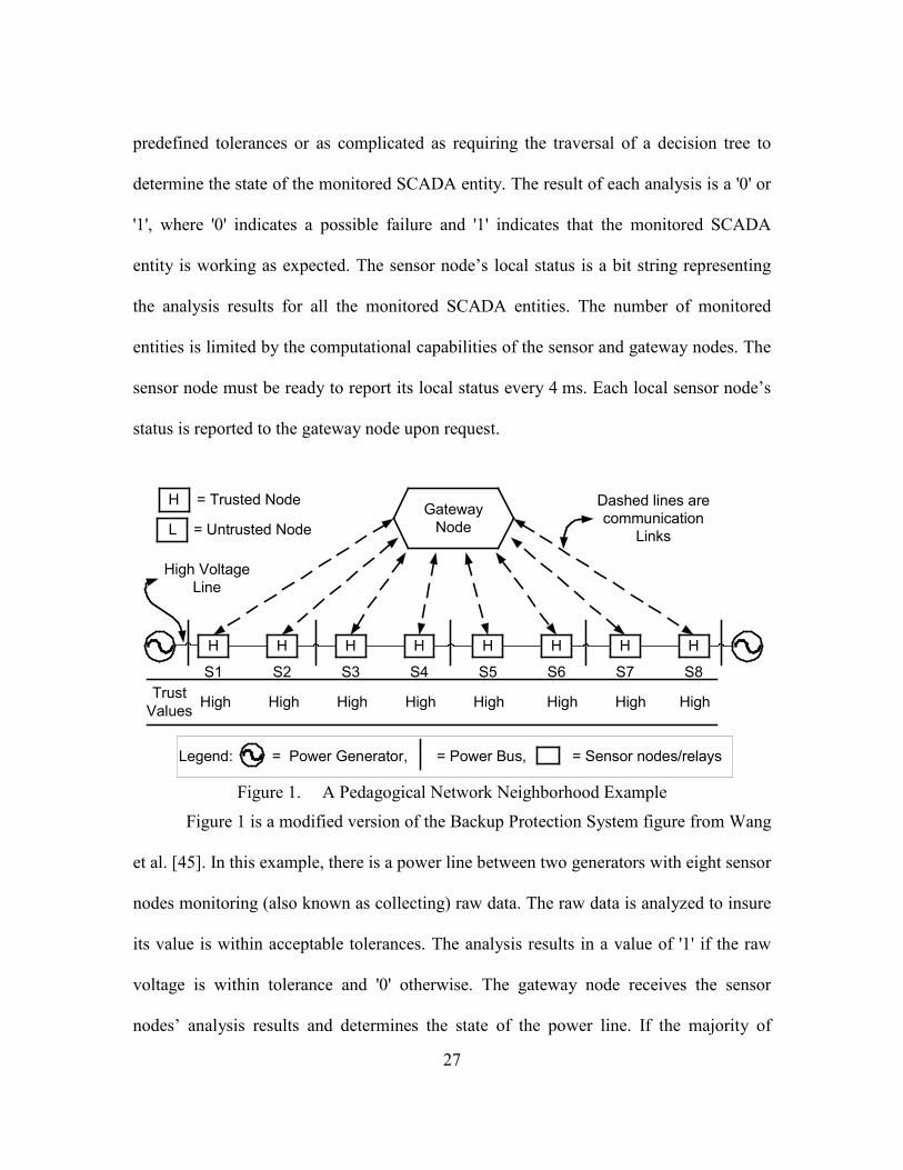
within a network neighborhood, see Figure 1. Sensor nodes monitor and analyze each
sensed SCADA entity, such as, line voltages, currents and impedances. The gateway
node evaluates the analyzed results from the sensor nodes and assigns trust values
accordingly. The SCADA entities monitored by these sensor nodes are predetermined
physical aspects of the power production and distribution system. For example, a sensor
node attached to a power line could monitor the voltage level flowing across the power
line. This monitored voltage is analyzed to determine if a fault condition exists. Each
sensor node’s result is transferred to the gateway node. The gateway node evaluates the
results from all the sensor nodes to determine and assign each sensor node a trust value.
The sensor nodes may collect multiple raw data readings from multiple SCADA
entities for analysis. The analysis performed depends on the type of SCADA entity being
monitored. For example, the analysis of a voltage reading may require a sensor node to
calculate its peak, average or RMS value. The results of this analysis are then evaluated.
Evaluation of the analyzed results could be as simple as insuring the results are within
27
predefined tolerances or as complicated as requiring the traversal of a decision tree to
determine the state of the monitored SCADA entity. The result of each analysis is a '0' or
'1', where '0' indicates a possible failure and '1' indicates that the monitored SCADA
entity is working as expected. The sensor node’s local status is a bit string representing
the analysis results for all the monitored SCADA entities. The number of monitored
entities is limited by the computational capabilities of the sensor and gateway nodes. The
sensor node must be ready to report its local status every 4 ms. Each local sensor node’s
status is reported to the gateway node upon request.
Figure 1. A Pedagogical Network Neighborhood Example
Figure 1 is a modified version of the Backup Protection System figure from Wang
et al. [45]. In this example, there is a power line between two generators with eight sensor
nodes monitoring (also known as collecting) raw data. The raw data is analyzed to insure
its value is within acceptable tolerances. The analysis results in a value of '1' if the raw
voltage is within tolerance and '0' otherwise. The gateway node receives the sensor
nodes’ analysis results and determines the state of the power line. If the majority of
GatewayNode
H
S1
H
S2
H
S3
H
S4
H
S5
H
S6
H
S7
H
S8
High High High High High High High HighTrustValues
Dashed lines arecommunication
Links
High VoltageLine
H = Trusted Node
L = Untrusted Node
Legend: = Power Generator, = Power Bus, = Sensor nodes/relays

28
analysis results from the trusted sensor nodes are '1', then the power line is within
tolerance. If the majority of analysis results from the trusted sensor nodes are '0', then the
power line is not within tolerance. If no majority is found (i.e., the number of '1' equals
the number of '0'), then the state of the power line is unknown and no trust values are
updated, i.e., previous trust values remain valid. The gateway node’s evaluation result is
used to determine and assign trust values to the sensor nodes. If the sensor node’s
analysis results agrees with the gateway’s evaluation result, then the sensor node is
trusted (i.e., trust value is high), otherwise the sensor node is untrusted (i.e., trust value is
low).
Each network neighborhood consists of one gateway node and a finite set of
sensor nodes. The gateway node receives each sensor node's local status. These local
statuses are evaluated by the gateway node. For example, consider a gateway node with 8
sensor nodes in its neighborhood with the local statuses shown in Table 2, where nodes
S1-S8 represent the sensor nodes and each sensor node’s local status is represented as the
decimal integer representation of their 7 bit analysis results. Each bit represents a
monitored entity’s analysis result, where a '1' indicates that the monitored entity is within
tolerance and a '0' indicates that the monitored entity is not within tolerance. These
monitor entities are line voltages, line currents, or line impedances. The trust evaluation
is a conditional bitwise sum, followed by a left shift of the resulting sum values and a
comparison with the current number of trusted nodes. The result of this evaluation is a
sensor node consensus concerning the system state of the monitored SCADA entities.
Initially, all eight sensor nodes are trusted (i.e., have a high trust value assigned) by the

29
gateway node, i.e., the “Trust Value (before)” column. Each trusted node’s 7 bit value is
added to the conditional bitwise sum, e.g., all eight ones in column b0 are added together.
The bitwise sums are shifted to the left, i.e., their values are doubled. These shifted values
are compared to the current number of trusted sensor nodes; namely, 8. If the shifted
values are greater than the number of current trusted nodes, then the corresponding
evaluation result is a '1', otherwise '0'.
Table 2. Example of Gateway node system status evaluation using 8 trusted sensor nodes.
node Local status b b6 b5 b4 b3 b2 b1 Trust Value
(before)
0 Trust Value (after) Monitored SCADA Entities
S1 12310 1 = 1 1 1 0 1 1 High High S2 12310 1 = 1 1 1 0 1 1 High High S3 10910 1 = 1 0 1 1 0 1 High High S4 710 0 = 0 0 0 1 1 1 High Low S5 710 0 = 0 0 0 1 1 1 High Low S6 1710 0 = 0 1 0 0 0 1 High Low S7 12310 1 = 1 1 1 0 1 1 High High S8 12310 1 = 1 1 1 0 1 1 High High
Conditional Bitwise Sum 5 5 5 5 3 6 8 Shifted Bitwise Sum 10 10 10 10 6 12 16
System Status Results 1 1 1 1 0 1 1 Note: The “Trust Value (before)” column contains the sensor node’s trust values before the Gateway evaluation algorithm
starts. The “Trust Value (after)” column contains the sensor node’s trust values after the Gateway evaluation algorithm.
The evaluation results represent the sensor nodes’ consensus concerning the state
of each monitored SCADA entity. Collectively the evaluation results are referred to as
the neighborhood system status. This system status is compared with the sensor nodes'
local state to determine the sensor nodes' trust values, i.e., the “Trust Value (after)”
column. If over half of the local status bits match the system status bits, then the
corresponding sensor node is trusted (i.e., is assigned a high trust value), otherwise

30
untrusted (i.e., is assigned a low trust value). This is a bit by bit comparison where the
number of matches is used to determine a sensor node's trust value.
The gateway node’s evaluation results represent the neighborhood’s system
status. This system status is used to determine the trustworthiness of the sensor nodes in
the neighborhood. The bit string representing the local status from each sensor node is
compared with the system status bit string. This comparison is a bitwise exclusive OR
operation. The number of ones in the resulting bit string is shifted to the left and
compared to the number of SCADA entities monitored by the sensor nodes to determine
the corresponding sensor node’s trustworthiness, i.e., trust value. For example, node S1 in
Table 2, has a resulting bit string of 0000000 (i.e., 1111011 XOR 1111011). The number
of ones in this bit string result is zero. The left shift of this zero value remains zero
indicating that node S1 is trusted. The same holds true for nodes S2, S7 and S8. Nodes S4
and S5 in Table 2, have a resulting bit string of 1111100 (i.e., 0000111 XOR 1111011).
The number of ones in this bit string result is 5. The left shift of this 5 value results in 10.
Ten is greater than 7 (the number of SCADA entities monitored by each sensor node)
indicating that nodes S4 and S5 are untrusted. Node S6 in Table 2 has a resulting bit
string of 1101010 (0010001 XOR 1111011). The number of ones in this bit string result
is 4. The left shift of this 4 value results in 8. Eight is greater than 7 indicating that node
S6 is untrusted. The remaining nodes are evaluated and found to be trusted. Hence, the
next gateway evaluation uses the five trusted sensor nodes’ local status to determine the
neighborhood system status. The newly calculated system status is then used to determine
the trustworthiness of all the sensor nodes.

31
Our proposed Simple Trust protocol utilizes the addition, left shift and
comparison operations in the analysis and evaluation of sensor node data to determine the
neighborhood’s system status and the trustworthiness of each sensor node in the
neighborhood. These operations are some of the fastest operations performed by
computing devices. These fast operations enable our Simple Trust protocol to meet the
4 ms critical event detection timing constraint.
2.5 Experimental Design
Our experimental design focused on answering two questions: 1) can our Simple
Trust protocol meet timing constraints in a wireless network and 2) which factors
(transmission medium, network bandwidth or number of untrusted nodes) most affects
our ability to determine the system status within SCADA timing constraints. Our
experimental design follows a 2k 46 factorial design without replication format [ ]. This
experimental design was chosen for its ability to attribute a percentage of effect to the
2-level factors regarding their measured results. This approach provides statistical
evidence to support our findings concerning the factors’ effects on system status
determination time. The system status determination time is one of the measured metrics.
The remaining metrics are system throughput, transaction time, request time and response
time. The Simple Trust protocol's ability to quickly determine the neighborhood's system
status is measured as the system status determination time. The mean value of this metric
is used to answer question 1. The remaining metrics are collected to help answer
question 2 and for diagnostic purposes, i.e., to help identify problem areas causing the

32
system to exceed the 4 ms timing constraint. Figure 2 is a pictorial representation of this
experimental design.
Our experimental data come from simulations conducted within Network
Simulator 2 (NS2) [32]. NS2 version 2.29 was used within Cygwin version 1.5.25-15
running over Windows XP service pack 3. The computer hosting these simulations was a
Dell OptiPlex 755 with 3.25 GB of RAM and a Quad Q9550 CPU running at 2.83 GHz.
NAM (the Network Animator) version 1.0a1 [47] was used to visualize network
interactions.
This experiment varies the transmission medium, the bandwidth of the medium
and the number of untrusted nodes in the network. These three items were selected as the
factors of the experiment to help answer our two experiment questions. The two levels of
these factors are wired and wireless for the transmission medium type, 11 and 54 Mbps
bandwidths, and 1 or 3 untrusted nodes in the network.
Figure 2. Design of Experiment Block Diagram
A predefined workload scenario is submitted to the SUT with 1 of 8 possible
factor configurations, following a 2k
A B C
Predefined networktopology and workload scenario:8 sensor nodes and 1 gateway node
Throughput
System Status
Transaction
Request
Response
System Under Test (SUT)
NS2
NAM
Component Under TestMedium
32-bit Windows OS using Cygwin
factorial design. The factors labeled A, B and C
represent transmission medium, bandwidth and the number of untrusted nodes,

33
respectively. The collected metrics are system throughput, system status determination
time, transaction time, request time and response time. The SUT components represent
some of the experimental environment software elements.
2.6 Experimental Results
The results of our experiments show that the number of untrusted nodes has no
effect on the metric values. Furthermore, the 54 Mbps scenarios met the critical time
constraints and the 11 Mbps scenarios did not meet the critical timing constraints, see
Table 3. Further investigation is required to isolate the cause for the long system status
determination times at 11 Mbps. A small, approximately 2 percent, difference between
wired and wireless transmission mediums was observed in the 11 Mbps scenarios.
Possible causes of this small difference are queuing delays in the wired medium,
differences in packet sizes and the use of “request to send/clear to send” packets in the
wireless medium. There was no observed difference between wired and wireless
transmission mediums in the 54 Mbps scenarios, see Figure 3 and Figure 4. The 2k
Table 3. The mean System Status Determination Times.
factorial designed showed that of the three factors, bandwidth has a 99.9% effect on the
system status determination time. Hence, changes in bandwidth have the greatest impact
on our Simple Trust protocol’s ability to meet the 4 ms timing constraint.
Medium 11 Mbps 54 Mbps
1 bad node
3 bad nodes
1 bad node
3 bad nodes
Wired 5.56 ms 5.56 ms 2.4 ms 2.4 ms Wireless 5.44 ms 5.44 ms 2.4 ms 2.4 ms
Note: The 54 Mbps test scenarios met the 4 ms critical timing constraints [25]. The 11 Mbps test scenarios did not meet the timing constraints. The number of bad (untrusted) nodes had no affect on this —or any other—metric value.

34
2.7 Summary
In this section, we developed the Simple Trust protocol to allow for low
computational and bandwidth cost in evaluating trust between SCADA components. We
demonstrated the benefits of our Simple Trust protocol through simulation. The lack of
security protection measures in originally designed SCADA systems creates a security
risk. Our Simple Trust protocol is a protection enhancement capable of assigning trust
values to SCADA components and partially reducing this security risk. This enhancement
improves the SCADA controller responses by insuring the accuracy of the sensed system
status. We conclude that the greatest affects to the system status determination time is the
available bandwidth in the transmission medium. Our results also show that the Simple
Trust protocol meets the timing constraints in both wired and wireless mediums given
enough bandwidth. Our preliminary results show promise for the future creation of a
Trust Management Toolkit, which can manage SCADA networks based on assigned trust
values in order to proactively mitigate SCADA threats, failures and other byzantine
vulnerabilities.

35
1 Bad Node 3 Bad Nodes
Wire
d
Wire
less
Figure 3. 54 Mbps System Status Determination Time
All four 54 Mbps test scenarios resulted in system status determination (SSD)
times within the 4 ms timing constraints [25]. The initial SSD time for the wireless
scenarios is slightly longer than the wired scenarios. The steady-state values for both
wired and wireless scenarios are the same.
Sample Number
Syst
em S
tate
D
eter
min
atio
n Ti
me
(Sec
onds
)
0 205 410 615 820 1025 12300.000
0.001
0.002
0.003
0.004
0.005
0.006
0.007
X X X
Sample Number
Syst
em S
tate
D
eter
min
atio
n Ti
me
(Sec
onds
)
0 205 410 615 820 1025 12300.000
0.001
0.002
0.003
0.004
0.005
0.006
0.007
X X X
Sample Number
Syst
em S
tate
D
eter
min
atio
n Ti
me
(Sec
onds
)
0 205 410 615 820 1025 12300.000
0.001
0.002
0.003
0.004
0.005
0.006
0.007
X X X
Sample Number
Syst
em S
tate
D
eter
min
atio
n Ti
me
(Sec
onds
)
0 205 410 615 820 1025 12300.000
0.001
0.002
0.003
0.004
0.005
0.006
0.007
X X X

36
1 Bad Node 3 Bad Nodes W
ired
Wire
less
Figure 4. 11 Mbps System Status Determination Time
All four 11 Mbps test scenarios resulted in system status determination (SSD)
times above the 4 ms timing threshold [25]. The wired 11 Mbps scenarios are very stable
compared to the wireless scenarios, which display a considerable amount of variation.
Sample Number
Syst
em S
tate
D
eter
min
atio
n Ti
me
(Sec
onds
)
0 205 410 615 820 1025 12300.000
0.001
0.002
0.003
0.004
0.005
0.006
0.007
X X X
Sample Number
Syst
em S
tate
D
eter
min
atio
n Ti
me
(Sec
onds
)
0 205 410 615 820 1025 12300.000
0.001
0.002
0.003
0.004
0.005
0.006
0.007
X X X
Sample Number
Syst
em S
tate
D
eter
min
atio
n Ti
me
(Sec
onds
)
0 205 410 615 820 1025 12300.000
0.001
0.002
0.003
0.004
0.005
0.006
0.007
X X X
Sample Number
Syst
em S
tate
D
eter
min
atio
n Ti
me
(Sec
onds
)
0 205 410 615 820 1025 12300.000
0.001
0.002
0.003
0.004
0.005
0.006
0.007
X X X

37
III. SCADA Trust Management System∗
Existing Supervisory Control and Data Acquisition (SCADA) systems were originally
designed for reliability. These initial SCADA systems used proprietary protocols over hub and
spoke modem enabled networks to access sensed data and initiate supervisory control. These
SCADA systems were not designed with Internet security in mind, which provides challenges as
these systems are migrated toward common Internet communication protocols and networks.
Traditional SCADA controllers react in an automated way that is oblivious to Internet attacks.
Such attacks can be identified and mitigated by the proposed SCADA Trust Management
System (TMS). SCADA TMS builds upon Simple Trust protocol to provide mission assurance,
via information integrity and information sharing within a SCADA network. Low computational
and bandwidth requirements are critically important to the success of SCADA TMS. SCADA
TMS has shown, through two Backup Protection System (BPS) Simulation test cases, the ability
to meet SCADA critical timing constraints and in one case improved response time by 99%.
3.1 Introduction
The protection of our nation’s critical infrastructures (e.g., electrical production and
distribution systems) has been deemed a matter of national security by the previous two
presidents and the current administration [7-11]. The 2003 blackout [1] affecting the North
Eastern United States and portions of Canada, showed us how important the electrical power grid
is to our way of life. In 2009 [6], Associated Press author Lauran Neergaard discussed how
improvements in medical technologies over the last decade have enabled people to move out of
∗ This chapter is based on the previously published paper, [48] J. E. Fadul, K. M. Hopkinson, T. R. Andel, J. T. Moore, and S. H. Kurkowski, "SCADA Trust Management System," in 2010 International Conference on Security and Management (SAM'10) (under The 2010 World Congress in Computer Science, Computer Engineering, and Applied Computing (WORLDCOMP'2010)), Las Vegas, Nevada USA, 2010, pp. 548 - 554.

38
nursing homes and use residential life support units. These people become dependent on their
electric powered medical equipment (.e.g., home oxygen machines and ventilators). These same
people may become collateral damage in a cyber war involving our nation’s electrical production
and distribution systems—power grid. The strategic use of cyber to achieve a tactical goal, e.g.
denial of power to a given area, may disrupt power to medical equipment used to keep home care
patients alive. Hence, a cyber war involving the nation’s power grid is a not just a matter of
national security, but also a matter of public health.
The reasons why our current electrical power grid is vulnerable to cyber attacks was
explained by Mr. Robert F. Dacey, in his 2004 testimony to Congress [49], where he identified
the following four causes:
1) the adoption of standardized technologies with known vulnerabilities,
2) the connectivity of control systems to other networks,
3) insecure remote connections, and
4) the widespread availability of technical information about control systems.
The importance of the nation’s power grid, coupled with their cyber vulnerabilities,
warrant its inclusion as one of our nation’s critical infrastructure (CI) requiring protection from
cyber attacks. This was confirmed by Melissa Hathaway and her team [12] in the 2009 cyber
space review.
This Supervisory Control and Data Acquisition (SCADA) Trust Management System
(TMS) is designed to protect power grid SCADA systems from cyber attacks. This additional
security is provided via information assurance’s; information integrity, sharing and
dissemination within the SCADA network. Some may think a network firewall is sufficient for
the protection of SCADA networks, but improvements in technology and the increased computer

39
literacy throughout the world have increased the number of people capable of breaching network
firewalls [49]. Once past this firewall, the cyber attacker could manipulate the power grid to
achieve their goals. SCADA TMS does not replace or eliminate the need for a network firewall,
but supplements the use of a firewall by using side-channel information to verify detected faults
and determine corrective actions.
These cyber attacks may result in undesired actions; e.g., loss of power production, loss
of power distribution, or over production of power. Such undesired actions may result in loss of
revenue, damage to the environment and/or endangering the public’s safety [44]. The authors of
[44] have identified three challenges that must be addressed to strengthen legacy SCADA
networks; 1) improve access control, 2) improve security inside the SCADA network and 3)
improve security management. The second challenge corresponds to trusting the information
shared within a SCADA network and used in decision making. We are contributing to the
solution of this second SCADA challenge.
The remaining 5 sections are organized as follows; Section 3.2 contains background
information concerning SCADA and information concerning the development of trust,
Section 3.3 describes SCADA TMS, Section 3.4 describes two backup protection system (BPS)
test scenarios, Section 3.5 presents test results and the conclusion is presented in Section 3.6.
3.2 Background and Related Work
3.2.1 Background.
Typical power production and distribution systems consist of multiple components, see
Figure 5. A detailed explanation of all these components is beyond the scope of this research, but
a brief introduction proves useful in understanding the problem SCADA TMS is attempting to
solve.

40
Electrical energy is produced by a generating station. This electrical energy is
up-converted to a high voltage value by a step-up transformer located at the transmission
substation. This high voltage value minimizes power losses in transmission of electrical energy
over long distances. High voltage energy is transferred from the transmission substation to power
substations by high voltage transmission lines. A step-down transformer located at the power
substation down converts the received voltage to a lower value, normally a few thousand volts.
Distribution lines carry the voltage energy from the power substation to the customers. At the
customer’s location, a power step-down transformer converts the voltage energy to 120 volts and
240 volts before it enters the consumer’s home or office. This process is a very simplified view
of a power production and distribution system based on the information found in [1] and [50].
Multiple SCADA sensors and actuators are located throughout the system to monitor and control
power generation and distribution. The SCADA system controls the amount of power generated
to meet user demands, while insuring the power distribution system is not overloaded.
Figure 5. Power Production and Distribution System image by J. Messerly [1]
Figure 5 is a very simplified view of the power production and distribution system, which
does not consider line or component loss due to resistance or multiple paths from sources to
sinks.
Transmission lines 765, 500, 345, 230, and 138 kV
Transmission Customer 138kV or 230kV
Generating Station
Generating Step Up
Transformer
Substation Step Down
Transformer Color Key: Black: Generation Green: Distribution Blue: Transmission Subtransmission
Customer 26kV and 69kV
Primary Customer 13kV and 4kV
Secondary Customer 120V and 240V

41
The power industry, partnered with the United States government, is developing smart
grid technology and standards to help mitigate the increased electrical power demands and cyber
security threats [51]. The current power grid is a global broadcast system, where generators
supply power to the power grid’s transmission / distribution system and customers extract power
from the power grid’s transmission / distribution system. Originally, SCADA systems were
designed to monitor and control the electricity flowing in the power grid’s production and
distribution system to ensure safe and reliable service. SCADA system vulnerabilities were
limited to physical attacks, equipment failures and natural disasters (weather, tree limits,
woodpeckers … etc). Cyber attacks were not a legacy SCADA system design consideration.
Cost savings and efficiencies associated with advancements in communications
technologies have driven the power grid distribution system toward an Internet accessible
network. These advancements replaced costly proprietary protocols over serial Modbus
communication links with standard TCP/IP protocols. These advances provide real-time system
status to decision makers, e.g., system engineers and utility managers. These cost savings and
efficiencies gains come with an increased risk of cyber vulnerabilities.
A Government Accountability Office (GAO) study [22], see Figure 6, shows the number
of cyber attacks against our nation’s energy and power companies have increased over the years.
This alarming fact supports the presidential directives [7-11] issued by the previous two
presidents and the current administration, which identify the need to protect our nation’s power
grid from cyber attacks. SCADA TMS is designed to satisfy this need.

42
Figure 6. Government Accountability Office (GAO) Study [22]
Figure 6 depicts a GAO study showing an increase in cyber-attacks against U.S. energy
and power companies. In fact, a 2002 GAO report [52] stated that U.S. companies were attacked
an average of 1,280 times per company over a 6 month period (January 1, 2002, to June 30,
2002) and that 70 percent of these U.S. energy and power companies experienced some kind of
severe cyber attack against their computing or energy management systems over this same time
frame.
3.2.2 Related Work.
The previous efforts of Marsh [53], Buchegger et al. [42], Zimmermann [40],
Blaze et al. [39], Housley et al. [41], Kamvar et al. [43], Hopkinson et al. [24], Wang et al. [45]
and Igure et al. [44] provided guidance on how to define trust in a SCADA network.
David Marsh [53] was one of the first authors to formally define and assign trust values to
software agents’ interactions. Matt Blaze et al. [39] coined the term “Trust Management

43
Problem.” This term refers to the framework used to study security policies, security credentials
and trusted relationships. Matt Blaze et al. [39] work resulted in two software programs
(PolicyMaker and Keynote), which utilize Pretty Good Privacy (PGP) [40] and X.509 [41] for
individual authentication across a computer network.
CONFIDANT [42] and EigenTrust [43] protocols serve as inspiration for the initial
incarnation of SCADA TMS (i.e., Simple Trust protocol [30]). Also, the preliminary work by
Hopkinson et al. [24], Wang et al. [45] and Igure et al. [44], where agents within SCADA
systems were shown (via computer simulation) to be a viable cyber security preventative option.
3.3 SCADA Trust Management System
SCADA TMS consist of two major functions. Function one assigns trust values to
individual power production and distribution system components. Function two uses this trust
information in determining the correct course of action when a fault is detected. Software
entities, known as agents, perform these two functions. In our simulations, these trust agent
software programs are resident on intelligent electronic devices (IEDs) located at transmission
and power substation buses. The electrical buses located at the transmission and power
substations monitor and control the amount of electrical energy entering and leaving the power
transmission system—hence, our decision to locate trust agents at these power bus locations.
Information assurance is a key requirement of SCADA TMS. The information gathered
by trust agents, concerning the state of the transmission system’s power lines, is verified and
shared with other trust agents. A majority rules technique is used to verify the power system’s
state. The power system’s state is compared with the individual trust agents’ reported states to
determine their associated trust values. This verified state information is also shared with other

44
trust agents to mitigate false positives and false negatives. This description is a high level view
of our previously developed Simple Trust protocol—discussed in chapter 2 and in [30].
SCADA TMS uses trust information to make better decisions concerning detected fault
resolutions. The trust values initially developed using Simple Trust protocol discussed in
chapter 2 and in [30], are further refined using network flow techniques (e.g., image
segmentation or image labeling) to prevent false positive and false negative trust assignments. A
false positive is defined to be a non-malicious trust agent assigned a low trust value. A false
negative is defined as a malicious trust agent assigned a high trust value.
The image segmentation [27] network flow formulation, see Figure 7, is used to assign a
high or low trust value to the sensor nodes/relays. The image labeling [27] network flow
formulation, see Figure 8, is used to assign a percentage of trust, between 0 and 100, to the
sensor nodes/relays. This range of trust values considers the sensor node/relay’s previous 10 trust
values in determining its current trust value. Many network flow solvers exist, such as, the Ford-
Fulkerson labeling algorithm [54], for solving these network flow formulation problems.
SCADA TMS uses a modified version of the HIgh-level Push-Relabel (HIPR) flow
algorithm [55] to solve the resulting network flow formulation problems, see Appendix B. The
modifications to this program consists of adding an algorithm, by Curet et al. [56], for finding all
minimum cutsets. A minimum cutset partitions the network’s sensor node/relays into two sets, a
trusted set and an untrusted set. The minimum cutset is found by determining the minimal sum of
arcs(i,j), where i represents a node on the super source side of the cut and j represents a node on
the super sink side of the cut (for a more detail explanation of a minimum cutset see page 49).
The nodes on the super source side are trusted and the nodes on the super sink side are
untrusted. The resulting trust information is used by SCADA TMS decision making process.

45
Figure 7. Image Segmentation explanatory example
The arc capacities aj, bi, and pi,j Figure 7in represent the likelihood that node j is
trustworthy, the likelihood that node i is untrustworthy, and the penalty assessed for trusting
node i and not trusting an adjacent node j, respectively. Figure 7 also shows sensor node/relay,
S1, is assigned a High trust value and sensor node/relay, S2, is assigned a Low trust value. In
other words, the sensor nodes/relays on the source side of the cut are trusted, and the nodes on
the sink side of the cut are untrusted.
The initially developed trust values, along with the SCADA network topology, are
provided to Gateway nodes. This information is used by a parameter generator function, i.e.,
Parameter_Generator(Initial_values, SCADA_Network_Topology).
The parameter generator function sets up the abstract network flow parameters in accordance
with the detected fault. If no fault or a zone 1 fault is detected, then set up the parameters for an
image labeling network flow problem. Furthermore, if a zone 1 fault is detected, then use the
image labeling results to determine whether or not to trip its breakers. If a zone 3 fault is
detected, then set up the parameters for an image segmentation network flow problem to
determine the trusted breakers to trip. This information is provided to a modified HIPR
S1
S2
SuperSource
SuperSink
a1
a2
b1
b2
p12
p21
The Cut

46
program [55], which returns all the minimum cutsets within the given image segmentation or
image labeling networks. The original HIPR program returned one minimum cutset, although
multiple minimum cutsets existed. This solution was not useful for SCADA TMS
implementation. The algorithm for finding all minimum cutsets by Curet et al. [56] was added to
HIPR. This addition enables SCADA TMS to select the correct minimum cutset when multiple
minimum cutsets are found.
Image segmentation and image labeling attempt to maximize the flow from the added
super source node to the added super sink node. The difference between these two network flow
formulation techniques is the objective functions and the level of trust they can determine. The
image segmentation technique can separate the sensor node/relays into two groups, trusted and
untrusted. The image labeling technique can separate the sensor nodes/relays into multiple
groups (six groups are shown in Figure 8), where each group represents a level of trust. The
possible levels of trust for the sensor nodes in Figure 8 are 0% to 100% in 20% increments.
Figure 8. Modified image labeling explanatory example from [27]
S1,1 S1,3S1,2 S1,4 S1,5
S T
S2,1 S2,3S2,2 S2,4 S2,5
L
L L L L
L
LLLLL
La1,0
a1,1 a1,2 a1,3 a1,4
a1,5
a2,0 a2,1 a2,2 a2,3 a2,4a2,5
The Cut
p1,2 p1,2
p1,2
p1,2p1,2

47
The arc capacities aj,k, pi,j Figure 8 and L shown in represent the likelihood that node j is
assigned a k level of trust, the penalty assessed for assigning adjacent nodes i and j different k
levels of trust, and the amount of return flow, respectively. Nodes S and T represent the Super
Source and Super Sink nodes, respectively. Figure 8 shows sensor node/relay S1 is assigned an
80% trust k value and sensor node/relay S2 is assigned a 40% trust k value. A predefined
threshold of 75% may be used for determining trusted and untrusted sensor node/relays.
The network flow objective function being maximized by image segmentation is:
Maximize: 𝜈 (1)
Subject to:
� 𝑓�𝑆𝑖, 𝑆𝑗�𝑆𝑗∈𝐴(𝑆𝑖)
− � 𝑓(𝑆𝑘 ,𝑆𝑖)𝑆𝑘∈𝐵(𝑆𝑖)
= �𝜈 𝑖𝑓 𝑆𝑖 == 𝑆𝑜𝑢𝑟𝑐𝑒0 𝑖𝑓 𝑆𝑖 ≠ 𝑆𝑜𝑢𝑟𝑐𝑒 ∧ 𝑆𝑖 ≠ 𝑆𝑖𝑛𝑘
−𝜈 𝑖𝑓 𝑆𝑖 == 𝑆𝑖𝑛𝑘�
(also known as Conservation Constraints)
(2)
𝑓�𝑆𝑖, 𝑆𝑗� ≤ 𝑎𝑗 𝑖𝑓 𝑆𝑖 == 𝑆𝑜𝑢𝑟𝑐𝑒 (3)
𝑓�𝑆𝑖, 𝑆𝑗� ≤ 𝑝𝑖,𝑗 𝑖𝑓 𝑆𝑖 ≠ 𝑆𝑜𝑢𝑟𝑐𝑒 ∧ 𝑆𝑗 ≠ 𝑆𝑖𝑛𝑘 (4)
𝑓�𝑆𝑖, 𝑆𝑗� ≤ 𝑏𝑖 𝑖𝑓 𝑆𝑗 == 𝑆𝑖𝑛𝑘 (5)
𝑓�𝑆𝑖, 𝑆𝑗� ≥ 0 (6)
where
𝑁 is the set of nodes in the network
𝐴𝑟𝑐𝑠 is the set of arcs in the network
|𝑁| ∈ ℕ ∪ {0} is the cardinality of set 𝑁
𝑖, 𝑗,𝑘 ∈ {1 … |𝑁|} are node index variables used to specify individual nodes in the network
𝜈 is the maximum flow from the source node to the sink node, such that
𝜈 = � 𝑓�𝑆𝑜𝑢𝑟𝑐𝑒, 𝑆𝑗� = � 𝑓(𝑆𝑖, 𝑆𝑖𝑛𝑘)𝑆𝑖∈𝐵(𝑆𝑖𝑛𝑘)𝑆𝑗∈𝐴(𝑆𝑜𝑢𝑟𝑐𝑒)
also known as Capacity
Constraints

48
𝐴: 𝑆𝑖 → 𝑁 is a function mapping a given node 𝑆𝑖 ∈ 𝑁 to a set of nodes 𝑆𝑗 ∈ 𝑁 that are
after 𝑆𝑖, i.e. ⟨𝑆𝑖, 𝑆𝑗⟩ ∈ 𝐴𝑟𝑐𝑠.
In other words, 𝐴(𝑆𝑖) = �𝑆𝑗 ∈ 𝑁|⟨𝑆𝑖,𝑆𝑗⟩ ∈ 𝐴𝑟𝑐𝑠�
𝐵: 𝑆𝑗 → 𝑁 is a function mapping a given node 𝑆𝑗 ∈ 𝑁 to a set of nodes 𝑆𝑖 ∈ 𝑁 that are
before 𝑆𝑗, i.e. ⟨𝑆𝑖, 𝑆𝑗⟩ ∈ 𝐴𝑟𝑐𝑠.
In other words, 𝐵�𝑆𝑗� = �𝑆𝑖 ∈ 𝑁|⟨𝑆𝑖, 𝑆𝑗⟩ ∈ 𝐴𝑟𝑐𝑠�
𝑓:𝐴𝑟𝑐𝑠 → ℝ is a function mapping network arcs to real value which represent the flow
across the specific arc.
𝑎𝑗 is the capacity of arc ⟨𝑆𝑖, 𝑆𝑗⟩ where 𝑆𝑖 = 𝑆𝑜𝑢𝑟𝑐𝑒 and represents the
likelihood that node 𝑆𝑗 is trustworthy
𝑏𝑖 is the capacity of arc ⟨𝑆𝑖, 𝑆𝑗⟩ where 𝑆𝑗 = 𝑆𝑖𝑛𝑘 and represents the likelihood
that node 𝑆𝑖 is not trustworthy
𝑝𝑖,𝑗 is the capacity of arc ⟨𝑆𝑖, 𝑆𝑗⟩ where 𝑆𝑖 ≠ 𝑆𝑜𝑢𝑟𝑐𝑒 and 𝑆𝑗 ≠ 𝑆𝑖𝑛𝑘 and
represents the penalty assessed for separating adjacent nodes 𝑆𝑖 and 𝑆𝑗 into
separate trust categories, e.g. 𝑆𝑖 is trusted and 𝑆𝑗 is not trusted or vice versa.
Solving this network flow problem for its maximum flow value, from the source node to the sink
node, results in a flow value 𝜈 and a partitioning of the network into two parts; namely a source
side partition and a sink side partition. The network nodes on the source side of the partition are
considered trustworthy and the network nodes on the sink side of the partition are considered
untrustworthy. This partitioning of the network is called the minimum 𝑠 − 𝑡 cutset and represents
the dual of the maximum flow from 𝑠 to 𝑡, where 𝑠 is the source node and 𝑡 is the sink node.

49
This duality is referred to as the maximum flow-minimum cut theorem [27, 54, 57, 58]. The
corresponding dual network flow objective function being minimized, with its constraints, is:
Minimize: ��𝑢�𝑆𝑖, 𝑆𝑗�ℎ�𝑆𝑖, 𝑆𝑗�|𝑁|
𝑗=1
|𝑁|
𝑖=1
(7)
Subject to: 𝑢�𝑆𝑖, 𝑆𝑗� = 0 𝑖𝑓 ⟨𝑆𝑖, 𝑆𝑗⟩ ∉ 𝐴𝑟𝑐𝑠 (8)
𝑢�𝑆𝑖, 𝑆𝑗� = 𝑏𝑖 𝑖𝑓 𝑆𝑖 ∈ 𝑋 and 𝑆𝑗 == 𝑆𝑖𝑛𝑘 (9)
𝑢�𝑆𝑖, 𝑆𝑗� = 𝑎𝑗 𝑖𝑓 𝑆𝑖 == 𝑆𝑜𝑢𝑟𝑐𝑒 and 𝑆𝑗 ∈ 𝑋� (10)
𝑢�𝑆𝑖, 𝑆𝑗� = 𝑝𝑖,𝑗 𝑖𝑓 𝑆𝑖 ∈ 𝑋 and 𝑆𝑖 ≠ 𝑆𝑜𝑢𝑟𝑐𝑒 and 𝑆𝑗 ∈ 𝑋� and 𝑆𝑗 ≠ 𝑆𝑖𝑛𝑘 (11)
ℎ�𝑆𝑖, 𝑆𝑗� ≥ 0 𝑖𝑓 ⟨𝑆𝑖, 𝑆𝑗⟩ ∈ (𝑋,𝑋�) 𝑡ℎ𝑒𝑛 ℎ�𝑆𝑖, 𝑆𝑗� = 1 𝑜𝑡ℎ𝑒𝑟𝑤𝑖𝑠𝑒 0 (12)
where
𝑋 is the set of nodes on the source side of the cut, 𝑆𝑜𝑢𝑟𝑐𝑒 ∈ 𝑋, and represent the
set of trustworthy nodes, such that
𝑋 = 𝑁 − 𝑋� and 𝑋� = 𝑁 − 𝑋 and 𝑋 ∩ 𝑋� = ∅
𝑋� is the set of nodes on the sink side of the cut, 𝑆𝑖𝑛𝑘 ∈ 𝑋�, and represent the set
of untrustworthy nodes, such that
𝑋 = 𝑁 − 𝑋� and 𝑋� = 𝑁 − 𝑋 and 𝑋 ∩ 𝑋� = ∅
(𝑋,𝑋�) is the set of arcs, ⟨𝑆𝑖, 𝑆𝑗⟩, where 𝑆𝑖 ∈ 𝑋 and 𝑆𝑗 ∈ 𝑋�
𝑢:𝐴𝑟𝑐𝑠 → ℝ is a function mapping arcs to real values and represent the arc’s capacity
ℎ:𝐴𝑟𝑐𝑠 → {0,1} is a selection function from the set of 𝐴𝑟𝑐𝑠 to a binary value, such that
ℎ�𝑆𝑖, 𝑆𝑗� = �1 𝑖𝑓 ⟨𝑆𝑖, 𝑆𝑗⟩ ∈ (𝑋,𝑋�)0 𝑜𝑡ℎ𝑒𝑟𝑤𝑖𝑠𝑒
�

50
The network flow objective function being maximized by image labeling is:
Maximize: 𝜈 (13)
Subject to: � 𝑓�𝑆𝑖,𝑘,𝑆𝑗,𝑙� − � 𝑓�𝑆𝑧,𝑦, 𝑆𝑖,𝑘� = �
𝜈 𝑖𝑓 𝑆𝑖,𝑘 == 𝑆𝑜𝑢𝑟𝑐𝑒0 𝑖𝑓 𝑆𝑖,𝑘 ≠ 𝑆𝑜𝑢𝑟𝑐𝑒 ∧ 𝑆𝑖,𝑘 ≠ 𝑆𝑖𝑛𝑘
−𝜈 𝑖𝑓 𝑆𝑖,𝑘 == 𝑆𝑖𝑛𝑘�
𝑆𝑧,𝑦∈𝐵�𝑆𝑖,𝑘�𝑆𝑗,𝑙∈𝐴�𝑆𝑖,𝑘�
(also known as Conservation Constraints)
(14)
𝑓�𝑆𝑖,𝑘, 𝑆𝑗,𝑙� ≤ 𝑎𝑗,0 𝑖𝑓 𝑆𝑖,𝑘 == 𝑆𝑜𝑢𝑟𝑐𝑒 (15)
𝑓�𝑆𝑖,𝑘, 𝑆𝑗,𝑙� ≤ 𝐿 𝑖𝑓 𝑆𝑗,𝑙 == 𝑆𝑜𝑢𝑟𝑐𝑒 (16)
𝑓�𝑆𝑖,𝑘, 𝑆𝑗,𝑙� ≤ 𝑝𝑖,𝑗 𝑖𝑓 𝑆𝑖,𝑘 ≠ 𝑆𝑜𝑢𝑟𝑐𝑒 ∧ 𝑆𝑗,𝑙 ≠ 𝑆𝑖𝑛𝑘 ∧ 𝑘 == 𝑙 ∧ 𝑖 ≠ 𝑗 (17)
𝑓�𝑆𝑖,𝑘, 𝑆𝑗,𝑙� ≤ 𝑎𝑖,𝑘 𝑖𝑓 𝑆𝑗,𝑙 ≠ 𝑆𝑖𝑛𝑘 ∧ 𝑙 == 𝑘 + 1 ∧ 𝑖 == 𝑗 (18)
𝑓�𝑆𝑖,𝑘, 𝑆𝑗,𝑙� ≤ 𝐿 𝑖𝑓 𝑆𝑗,𝑙 ≠ 𝑆𝑜𝑢𝑟𝑐𝑒 ∧ 𝑙 == 𝑘 − 1 ∧ 𝑖 == 𝑗 (19)
𝑓�𝑆𝑖,𝑘, 𝑆𝑗,𝑙� ≤ 𝑎𝑖,𝑘 𝑖𝑓 𝑆𝑗,𝑙 == 𝑆𝑖𝑛𝑘 (20)
𝑓�𝑆𝑖,𝑘, 𝑆𝑗,𝑙� ≤ 𝐿 𝑖𝑓 𝑆𝑖,𝑘 == 𝑆𝑖𝑛𝑘 (21)
𝑓�𝑆𝑖,𝑘, 𝑆𝑗,𝑙� ≥ 0 (22)
Also known as Capacity
Constraints

51
where
𝑁 is the set of nodes in the network
𝐴𝑟𝑐𝑠 is the set of arcs in the network
|𝑁| ∈ ℕ ∪ {0} is the cardinality of set 𝑁
𝑖, 𝑗, 𝑧 ∈ {1 … |𝑁|} are node index variables used to specify individual nodes in the
network
𝑀 is the number of trust levels
𝑙,𝑘,𝑦 ∈ {0 …𝑀} are trust level index variables used to specify an individual node’s
trust level
𝜈 is the maximum flow from the source node to the sink node, such
that 𝜈 = � 𝑓�𝑆𝑜𝑢𝑟𝑐𝑒, 𝑆𝑗,𝑙� = � 𝑓�𝑆𝑖,𝑘,𝑆𝑖𝑛𝑘�𝑆𝑖,𝑘∈𝐵(𝑆𝑖𝑛𝑘)𝑆𝑗,𝑙∈𝐴(𝑆𝑜𝑢𝑟𝑐𝑒)
𝐴: 𝑆𝑖,𝑘 → 𝑁 is a function mapping a given node 𝑆𝑖,𝑘 ∈ 𝑁 to a set of nodes
𝑆𝑗,𝑙 ∈ 𝑁 that are after 𝑆𝑖,𝑘, i.e. ⟨𝑆𝑖,𝑘,𝑆𝑗,𝑙⟩ ∈ 𝐴𝑟𝑐𝑠.
In other words, 𝐴�𝑆𝑖,𝑘� = �𝑆𝑗,𝑙 ∈ 𝑁|⟨𝑆𝑖,𝑘, 𝑆𝑗,𝑙⟩ ∈ 𝐴𝑟𝑐𝑠�
𝐵: 𝑆𝑗,𝑙 → 𝑁 is a function mapping a given node 𝑆𝑗,𝑙 ∈ 𝑁 to a set of nodes
𝑆𝑖,𝑘 ∈ 𝑁 that are before 𝑆𝑗,𝑙, i.e. ⟨𝑆𝑖,𝑘, 𝑆𝑗,𝑙⟩ ∈ 𝐴𝑟𝑐𝑠.
In other words, 𝐵�𝑆𝑗,𝑙� = �𝑆𝑖,𝑘 ∈ 𝑁|⟨𝑆𝑖,𝑘, 𝑆𝑗,𝑙⟩ ∈ 𝐴𝑟𝑐𝑠�
𝑓:𝐴𝑟𝑐𝑠 → ℝ is a function mapping network arcs to real value which represent the
flow across the specific arc.
𝑎𝑖,𝑘 is the capacity of arc ⟨𝑆𝑖,𝑘, 𝑆𝑗,𝑙⟩ where 𝑆𝑖,𝑘 ≠ 𝑆𝑜𝑢𝑟𝑐𝑒 and represents
the likelihood that node 𝑆𝑖,𝑘 is assigned k level of trust

52
𝑎𝑗,0 is the capacity of arc ⟨𝑆𝑖,𝑘, 𝑆𝑗,𝑙⟩ where 𝑆𝑖,𝑘 == 𝑆𝑜𝑢𝑟𝑐𝑒 and represents
the likelihood that node 𝑆𝑗,𝑙 is assigned a 0 level of trust, i.e. 𝑘 == 0
𝐿 is the capacity of the return arcs, 𝐿 ≥ ∑ 𝑎𝑗,0𝑆𝑗∈𝑁
Returns arcs are arcs that satisfy one of the following two conditions:
1) ⟨𝑆𝑖,𝑘, 𝑆𝑗,𝑙⟩ with 𝑆𝑖,𝑘 == 𝑆𝑖𝑛𝑘 or 𝑆𝑗,𝑙 == 𝑆𝑜𝑢𝑟𝑐𝑒
2) ⟨𝑆𝑖,𝑘, 𝑆𝑗,𝑙⟩ 𝑤𝑖𝑡ℎ 𝑆𝑗,𝑙 ≠ 𝑆𝑜𝑢𝑟𝑐𝑒 and 𝑆𝑖,𝑘 ≠ 𝑆𝑖𝑛𝑘 and 𝑙 == 𝑘 − 1
and 𝑖 == 𝑗
𝑝𝑖,𝑗 is the capacity of arc ⟨𝑆𝑖,𝑘, 𝑆𝑗,𝑙⟩ where 𝑆𝑖,𝑘 ≠ 𝑆𝑜𝑢𝑟𝑐𝑒 and 𝑆𝑗,𝑙 ≠ 𝑆𝑖𝑛𝑘
and 𝑙 == 𝑘 and 𝑖 ≠ 𝑗 and represents the penalty assessed for
assigning adjacent nodes different trust k levels.
As with the image segmentation [27] techniques discussed earlier, solving this image
labeling [27] network flow problem results in a maximum flow value 𝜈 and a partitioning
of the network into two parts; namely a source side partition and a sink side partition. As
previously mentioned, this partitioning of the network is called the minimum 𝑠 − 𝑡 cutset
and represents the dual of the maximum flow from 𝑠 to 𝑡, where 𝑠 is the source node and
𝑡 is the sink node. This process is referred to as the maximum flow-minimum cut
theorem [27, 54, 57, 58]. The resulting minimum cutset is used to assign k trust levels to
the network nodes, i.e. 𝑆𝑖 ∈ 𝑁 is assigned trust level k if and only if 𝑎𝑖,𝑘 ∈ (𝑋,𝑋�). The
corresponding dual network flow objective function being minimized with its constraints
is:

53
Minimize: �� � � 𝑢�𝑆𝑖,𝑘, 𝑆𝑗,𝑙�ℎ�𝑆𝑖,𝑘,𝑆𝑗,𝑙�|𝑁|+1
𝑗=0
|𝑁|+1
𝑖=0
𝑀
𝑙=0
𝑀
𝑘=0
(23)
Subject to: 𝑢�𝑆𝑖,𝑘,𝑆𝑗,𝑙� = 0 𝑖𝑓 ⟨𝑆𝑖,𝑘, 𝑆𝑗,𝑙⟩ ∉ 𝐴𝑟𝑐𝑠 (24)
𝑢�𝑆𝑖,𝑘,𝑆𝑗,𝑙� = 𝑎𝑗,0 𝑖𝑓 𝑆𝑖,𝑘 == 𝑆𝑜𝑢𝑟𝑐𝑒 (25)
𝑢�𝑆𝑖,𝑘,𝑆𝑗,𝑙� = 𝐿 𝑖𝑓 𝑆𝑗,𝑙 == 𝑆𝑜𝑢𝑟𝑐𝑒 (26)
𝑢�𝑆𝑖,𝑘,𝑆𝑗,𝑙� = 𝑎𝑖,𝑘 𝑖𝑓 𝑆𝑗,𝑙 ≠ 𝑆𝑖𝑛𝑘 and 𝑙 == 𝑘 + 1 and 𝑖 == 𝑗 (27)
𝑢�𝑆𝑖,𝑘,𝑆𝑗,𝑙� = 𝐿 𝑖𝑓 𝑆𝑗,𝑙 ≠ 𝑆𝑜𝑢𝑟𝑐𝑒 and 𝑙 == 𝑘 − 1 and 𝑖 == 𝑗 (28)
𝑢�𝑆𝑖,𝑘,𝑆𝑗,𝑙� = 𝑝𝑖,𝑗 𝑖𝑓 𝑆𝑖,𝑘 ≠ 𝑆𝑜𝑢𝑟𝑐𝑒 and 𝑆𝑗,𝑙 ≠ 𝑆𝑖𝑛𝑘 and 𝑘 == 𝑙 and 𝑖 ≠ 𝑗 (29)
𝑢�𝑆𝑖,𝑘,𝑆𝑗,𝑙� = 𝑎𝑖,𝑘 𝑖𝑓 𝑆𝑗,𝑙 == 𝑆𝑖𝑛𝑘 (30)
𝑢�𝑆𝑖,𝑘,𝑆𝑗,𝑙� = 𝐿 𝑖𝑓 𝑆𝑖,𝑘 == 𝑆𝑖𝑛𝑘 (31)
ℎ�𝑆𝑖,𝑘, 𝑆𝑗,𝑙� ≥ 0 𝑖𝑓 ⟨𝑆𝑖,𝑘, 𝑆𝑗,𝑙⟩ ∈ (𝑋,𝑋�) 𝑡ℎ𝑒𝑛 ℎ�𝑆𝑖,𝑘, 𝑆𝑗,𝑙� = 1 𝑜𝑡ℎ𝑒𝑟𝑤𝑖𝑠𝑒 0
(32)
where
𝑋 is the set of nodes on the source side of the cut, 𝑆𝑜𝑢𝑟𝑐𝑒 ∈ 𝑋, and
represent the set of trustworthy nodes, such that
𝑋 = 𝑁 − 𝑋� and 𝑋� = 𝑁 − 𝑋 and 𝑋 ∩ 𝑋� = ∅
𝑋� is the set of nodes on the sink side of the cut, 𝑆𝑖𝑛𝑘 ∈ 𝑋�, and represent
the set of untrustworthy nodes, such that
𝑋 = 𝑁 − 𝑋� and 𝑋� = 𝑁 − 𝑋 and 𝑋 ∩ 𝑋� = ∅
(𝑋,𝑋�) is the set of arcs, ⟨𝑆𝑖,𝑘, 𝑆𝑗,𝑙⟩, where 𝑆𝑖,𝑘 ∈ 𝑋 and 𝑆𝑗,𝑙 ∈ 𝑋�
𝑢:𝐴𝑟𝑐𝑠 → ℝ is a function mapping arcs to real values and represent the arc’s
capacity

54
ℎ:𝐴𝑟𝑐𝑠 → {0,1} is a selection function from the set of 𝐴𝑟𝑐𝑠 to binary value,
i.e. ℎ�𝑆𝑖,𝑘, 𝑆𝑗,𝑙� = �1 𝑖𝑓 ⟨𝑆𝑖,𝑘, 𝑆𝑗,𝑙⟩ ∈ (𝑋,𝑋�)0 𝑜𝑡ℎ𝑒𝑟𝑤𝑖𝑠𝑒
�
SCADA TMS implements the rules listed in Table 4 with the trust values
resulting from the network flow formulated problems. The two possible fault types are
zone 1 and zone 3 faults. A zone 1 fault is a line fault near the detecting relay and a
zone 3 fault is a line fault further away from the relay. The apparent line impedance
amount seen by the detecting relay is used to distinguish between zone 1 and zone 3
failures. A zone 1 failure detection is always accompanied by a zone 3 failure detection.
While a zone 3 failure detection may be far enough away that a zone 1 failure is not
detected. When a zone 1 trip signal is generated by a trusted agent, the SCADA TMS
attempts to locally confirm the signal by checking the zone 3 trip signal status, as well as
the voltages and currents on the power lines. If the zone 1 trip signal is confirmed locally,
then proceed to trip the breaker. If the zone 1 trip signal is not confirmed locally or the
source of the signal is an untrusted agent, then TMS blocks the signal and will request
confirmation from its nearby agents—via gateway nodes. If the zone 1 trip signal is not
confirmed by nearby agents, then SCADA TMS will continue to block the incorrect trip
signal. If the zone 1 trip signal is confirmed by neighboring agents, then SCADA TMS
will send a gateway trip signal, which engages the associated breaker.
When a zone 3 trip signal is generated by a trusted agent, SCADA TMS attempts
to locally confirm the signal by checking the voltages and currents on the distribution
lines. If the zone 3 trip signal is confirmed locally, then SCADA TMS awaits a gateway
trip signal before tripping the circuit breaker. This gives the zone 1 relays the opportunity
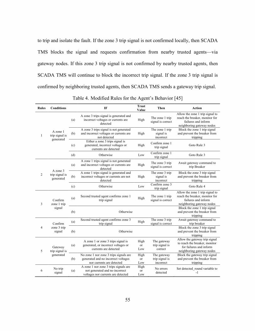
55
to trip and isolate the fault. If the zone 3 trip signal is not confirmed locally, then SCADA
TMS blocks the signal and requests confirmation from nearby trusted agents—via
gateway nodes. If this zone 3 trip signal is not confirmed by nearby trusted agents, then
SCADA TMS will continue to block the incorrect trip signal. If the zone 3 trip signal is
confirmed by neighboring trusted agents, then SCADA TMS sends a gateway trip signal.
Table 4. Modified Rules for the Agent’s Behavior [45]
Rules Conditions IF Trust Value Then Action
1 A zone 1
trip signal is generated
(a) A zone 3 trips signal is generated and
incorrect voltages or currents are detected
High The zone 1 trip signal is correct
Allow the zone 1 trip signal to reach the breaker, monitor for
failures and inform neighboring gateway nodes
(b) A zone 3 trips signal is not generated and incorrect voltages or currents are
not detected High
The zone 1 trip signal is incorrect
Block the zone 1 trip signal and prevent the breaker from
tripping
(c) Either a zone 3 trips signal is
generated, incorrect voltages or currents are detected
High Confirm zone 1 trip signal Goto Rule 3
(d) Otherwise Low Confirm zone 1 trip signal Goto Rule 3
2 A zone 3
trip signal is generated
(a) A zone 1 trips signal is not generated and incorrect voltages or currents are
detected High The zone 3 trip
signal is correct Await gateway command to
trip Breaker
(b) A zone 1 trips signal is generated and incorrect voltages or currents are not
detected High
The zone 3 trip signal is incorrect
Block the zone 3 trip signal and prevent the breaker from
tripping
(c) Otherwise Low Confirm zone 3 trip signal Goto Rule 4
3 Confirm
zone 1 trip signal
(a) Second trusted agent confirms zone 1 trip signal High The zone 1 trip
signal is correct
Allow the zone 1 trip signal to reach the breaker, monitor for
failures and inform neighboring gateway nodes
(b) Otherwise Block the zone 1 trip signal
and prevent the breaker from tripping
4 Confirm
zone 3 trip signal
(a) Second trusted agent confirms zone 3 trip signal High The zone 3 trip
signal is correct Await gateway command to
trip breaker
(b) Otherwise Block the zone 3 trip signal
and prevent the breaker from tripping
5 Gateway
trip signal is generated
(a) A zone 1 or zone 3 trips signal is
generated, or incorrect voltages or currents are detected
High or
Low
The gateway trip signal is
correct
Allow the gateway trip signal to reach the breaker, monitor
for failures and inform neighboring gateway nodes
(b) No zone 1 nor zone 3 trips signals are generated and no incorrect voltages
nor currents are detected
High or
Low
The gateway trip signal is
incorrect
Block the gateway trip signal and prevent the breaker from
tripping
6 No trip signal (a)
A zone 1 nor zone 3 trips signals are not generated and no incorrect
voltages nor currents are detected
High or
Low
No errors detected
Set detected_round variable to -1

56
3.4 Backup Protection System Scenarios
The originally designed hub and spoke modem enabled SCADA system is
abstractly represented in Figure 9. This representation shows two generators supplying
power to a high voltage transmission line. This high voltage line has 5 power buses and 8
sensor node/relays, where each relay controls a power line circuit breaker. The sensor
node/relays trip their associated circuit breaker when a predetermined fault condition is
detected or a trip circuit breaker message is received from the process control system.
The predetermined fault conditions are shorted power lines, large differential current
readings or low apparent resistance readings. Additionally, timing delays and pilot lines
are used to prevent cascading power outages. A point-to-point modem communication
system is used instead of the Wide Area Network (WAN) proposed in [24] and [45],
hence, the lack of information assurance’s integrity in fault conditions and received trip
messages. This lack of information integrity is a vulnerability that can be easily exploited
by a cyber attacker.
The proposed SCADA TMS, see Figure 10 and Figure 11, is an extension of [45],
designed to satisfy SCADA information assurance needs within acceptable timing
constraints. The timing constraints depend on the detected fault condition (e.g., a
lightning strike requires a faster system response than a received trip message from the
process control system). SCADA TMS adds an abstract software entity known as a
“gateway” node and modifies the sensor node/relay logic to utilize trust values, see
Table 4. The gateway nodes implement a Simple Trust protocol and uses network flow

57
techniques to determine and assign trust values to sensor node/relays. These trust values
are used to correctly mitigate detected faults.
Figure 9. Abstract Representation of a Legacy SCADA System
These test case scenarios consider the SCADA Backup Protection System (BPS).
SCADA BPS is designed to operate independently of primary protection systems. The
SCADA BPS relay engages its associated circuit breakers to isolate a detected fault not
mitigated by a primary protection system.
The two test case scenarios considered are 1) a false zone 1 trip signal generated
by a sensor node/relay and 2) a true trip signal ignored by three misbehaving sensor
node/relays. In the first test case scenario, a zone 1 trip signal is generated in error by
sensor node/relay S5. S5 is trusted by SCADA TMS. This indicates that the voltage and
current values reported by S5 agree with the neighboring reported values. The voltages
and currents are all within tolerance and no zone 3 trip signal is generated. This
information causes SCADA TMS to implement rule 1(b), i.e., block the false zone 1 trip
signal. Additionally, the SCADA BPS does not respond to the false zone 1 trip signal.
PROCESSCONTROLSYSTEM
R1 R2 R3 R4 R5 R6 R7 R8
Dashed lines arepoint to point modemcommunication Links
High VoltageLine
Legend: = Power Generator, = Power Bus, = relays

58
This test scenario is indicative of a cyber attacker gaining access to S5 and attempting to
trip the circuit breaker associated with S5 by generating a zone 1 trip signal.
Figure 10. Abstract Representation of SCADA TMS with all Trusted Nodes
Figure 11. Abstract Representation of SCADA TMS with Some Untrusted Nodes
PROCESSCONTROLSYSTEM
G1 G2 G3
H
S1
H
S2
H
S3
H
S4
H
S5
H
S6
H
S7
H
S8
High High High High High High High HighTrustValues
Dashed lines arecommunication
Links
High VoltageLine
H = Trusted Node
L = Untrusted Node
Legend: = Sensor nodes/relays, = Gateway Node,
= Power Generator, = Power Bus
G#
PROCESSCONTROLSYSTEM
G1 G2 G3
H
S1
H
S2
H
S3
H
S7
H
S8
High High High Low Low Low High HighTrustValues
Dashed lines arecommunication
Links
High VoltageLine
H = Trusted Node
L = Untrusted Node
Legend: = Sensor nodes/relays, = Gateway Node,
= Power Generator, = Power Bus
G#
L
S4
L
S6
L
S5

59
In the second test case, a true zone 1 trip signal is generated (i.e. a fault occurs on
the power line between sensor node/relays S5 and S6). In this scenario, sensor
node/relays S4, S5 and S6 are misbehaving and untrusted. This zone 1 trip signal is
ignored by S5 and S6, which causes the gateways G2 and G3 to engage the SCADA BPS
sensor node/relays, S3 and S7 (the nearest set of trusted sensor nodes/relays, see
Figure 11), to trip their circuit breakers. These SCADA BPS sensor node/relays S3 and
S7 comply with their received trip signals and trip their circuit breakers. The specifics on
how this works are as follows:
1) The true zone 1 trip signals at S5 and S6 are confirmed by zone 3 trip signals
and incorrect voltage and incorrect current readings.
2) Gateway nodes G2 and G3 received this information and the status of S5 and
S6 power line breakers. This information, together with predetermined trust
values, is used to select the nearest set of trusted sensor node/relays to respond
to the fault; namely, S3 and S7.
Sensor node/relays S3 and S7 are tasked by SCADA TMS as backup protection
sensor node/relays in this scenario. This test scenario is indicative of failed breaker
responses or cyber attacks against S4, S5 and S6 breakers.
3.5 Results
The results from the first test case scenario are shown in Figure 12 and Figure 13.
Figure 12 shows the false zone 1 signal generated at simulation time 0.2 seconds fails to
disrupt power flow. This signal is immediately blocked by SCADA TMS. Traditional
SCADA systems cannot confirm the integrity of the trip signal and result in an
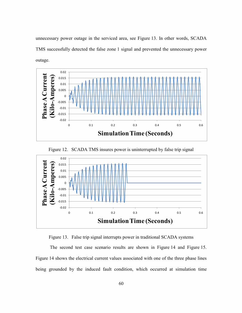
60
unnecessary power outage in the serviced area, see Figure 13. In other words, SCADA
TMS successfully detected the false zone 1 signal and prevented the unnecessary power
outage.
Figure 12. SCADA TMS insures power is uninterrupted by false trip signal
Figure 13. False trip signal interrupts power in traditional SCADA systems
The second test case scenario results are shown in Figure 14 and Figure 15.
Figure 14 shows the electrical current values associated with one of the three phase lines
being grounded by the induced fault condition, which occurred at simulation time
-0.02
-0.015
-0.01
-0.005
0
0.005
0.01
0.015
0.02
0 0.1 0.2 0.3 0.4 0.5 0.6
Phas
e A C
urre
nt
(Kilo
-Am
pere
s)
Simulation Time (Seconds)
-0.02
-0.015
-0.01
-0.005
0
0.005
0.01
0.015
0.02
0 0.1 0.2 0.3 0.4 0.5 0.6
Phas
e A C
urre
nt
(Kilo
-Am
pere
s)
Simulation Time (Seconds)

61
0.3 seconds. This fault condition is detected by SCADA TMS at simulation time
0.312 seconds and corrective action is taken at simulation time 0.322 seconds. SCADA
TMS was able to detect the fault condition, determine where the fault occurred, that the
primary sensor node/relays (S5 and S6) have not tripped their circuit breakers and select
the nearest set of trusted sensor nodes/relays (S3 and S7) to trip and isolate the fault
condition. SCADA TMS was able to determine and implement the proper backup
protection system (BPS) corrective action within 22 milliseconds. A traditional SCADA
system would have taken 1575 milliseconds [45] to isolate the fault under these same
conditions, see Figure 15. These results indicate a 99 % improvement in BPS response
time. SCADA TMS shared communications correctly assessed the situation and
determined which trusted sensor node/relays to engaged. SCADA TMS successfully
isolates the line for fault clearing.
Figure 14. SCADA TMS isolates faulty line quickly
-4-202468
0 0.2 0.4 0.6 0.8 1 1.2 1.4 1.6 1.8 2
Phas
e A
Curr
ent
(Kilo
-Am
pere
s)
Simulation Time (Seconds)

62
Figure 15. Traditional SCADA system isolates faulty line in ~1.5 seconds [45]
3.6 Conclusion
Proposed SCADA TMS improves upon traditional legacy SCADA systems
response time to detected line faults and provides some defense against cyber attacks.
The two test scenarios indicate that SCADA Backup Protection System (BPS) is not
degraded, i.e. the quick responses by primary relays to zone 1 trip signals are maintained
and the response of secondary relays to zone 3 trip signals are improved.
The shared information, received by the gateway nodes, together with network
flow techniques and power grid topology provides a rapid means of determining the trust
values of each sensor node/relay. These trust values are key factors in SCADA TMS
ability to determine which corrective action from Table 4 to take when a fault is detected.
-4-202468
0 0.2 0.4 0.6 0.8 1 1.2 1.4 1.6 1.8 2
Phas
e A
Curr
ent
(Kilo
-Am
pere
s)
Simulation Time (Seconds)

63
IV. Trust Management and Security in the Future Communication-Based “Smart” Electric Power Grid∗
New standards and initiatives in the U.S. electric power grid are moving in the
direction of a smarter grid. Media attention has focused prominently on smart meters in
distribution systems, but big changes are also occurring in the domains of protection,
control, and Supervisory Control And Data Acquisition (SCADA) systems. These
changes promise to enhance the reliability of the electric power grid and to allow it to
safely operate closer to its limits, but there is also a real danger concerning the
introduction of network communication vulnerabilities to so-called cyber attacks. This
section advocates the use of a reputation-based trust management system as one method
to mitigate such attacks. A simulated demonstration of the potential for such systems is
illustrated in the domain of backup protection systems. The simulation results show the
promise of this proposed technique.
4.1 Introduction
There have been a number of significant efforts in recent years to replace legacy
protection, control, and Supervisory Control And Data Acquisition (SCADA) systems in
the electric power grid with modern communication network alternatives. Legacy
technology uses relatively limited communication and proprietary protocols. New efforts
based on a modern communication network approach, and often employing Internet
protocols and equipment, include Utility Communications Architecture version 2.0 ∗ [59] J. E. Fadul, K. M. Hopkinson, T. R. Andel, and J. T. Moore, "Trust Management and Security in the Future Communication-Based “Smart” Electric Power Grid," in 44 Hawaii International Conference on System Sciences (HICSS) (Electric Power Systems: reliability, Security, and Trust Track), Koloa, Kauai, Hawaii, January 4-7, 2011, pp. 1-10.

64
(UCA 2.0) [60] in the 1990s followed by the IEC 61850 standard [61] and more recently,
the Wide Area Measurement System [62], NASPI [63], and the general push towards
“smart grid” technology [21]. While the media’s portrayal of smart grid is often
synonymous with smart metering, it can be defined more expansively to encompass
modern technologies for the power production and transmission system (also known as
power grid), such as those mentioned above. The holistic result of smart grid technology
is likely to be protection and control equipment that is more reliable and aware than its
predecessors. SCADA systems leveraging these smart grid technologies should be
capable of much faster sweeps through the grid with higher data transfer rates and
possibly include more information not previously provided.
The term “smart” in smart grid is perhaps misleading. It evokes images of a grid
that adapts its behavior through learning—using artificial intelligence methods to
improve its performance over time with little user monitoring or control. This type of
smart grid is unlikely since it would be too unpredictable to trust. A more realistic
description of the smart grid is a set of protection and control schemes that previously
operated on a stand-alone basis, with limited or no communication capabilities, which
will be able to use network communication capabilities to gain context-awareness about
the regional status of the grid. This context-awareness has the potential to greatly
improve the effectiveness of the protection and control schemes in question. A
disadvantage accompanying this new reliance on communication and digital software is
the potential increased risk to malicious network attacks, such as viruses, and other such
problems seen in the Internet, i.e., increased vulnerability to cyber attacks.

65
This section advocates the use of a reputation-based trust management system to
mitigate network vulnerabilities to cyber attacks in future smart electric power grids. A
basic approach towards this end is described using a communication-based backup
protection system as an example of how a trust management system can be introduced to
smart grid devices. A simulation is also conducted to illustrate the benefits of the
reputation-based trust management system.
4.2 Background
The blackout of 2003 [1] was a devastating blow to the United States (U.S.)
economy[4] [5], health [3] and safety [6]. Millions of citizens in the U.S. and Canada
were affected by this blackout [2], which is estimated to have cost the U.S. 6 billion
dollars. This is not surprising considering the loss of 61,800 Megawatts (MW) [2] of
electric power during the 2003 blackout is the largest power outage in U. S. history [3].
The devastating effects of this blackout could be caused by a cyber attack in the future, as
shown by the Department of Homeland Security (DHS) “Aurora Generator Test” [13].
This DHS demonstration highlighted the nation’s power grid vulnerability to cyber
attacks and prompted the move toward a smart electric power grid (also known as Smart
Grid). New Smart Grid technologies are intended to protect the nation’s power grid from
cyber attacks and improve overall efficiency to meet projected increases in energy
demands. The use of a reputation-based trust management system within the smart grid
will help meet these goals by assigning trust values to the sources of SCADA
information.

66
Our nation’s power grid supports and enables many safety services; such as public
and private transportation, and water treatment and distribution facilities. The 2003
blackout left ~1.5 million Cleveland Ohio residence without water for approximately
10 days. The water treatment and distribution facilities used electric water pumps. In
New York City, the 2003 blackout disabled the traffic signals causing multiple vehicle
accidents and traffic jams. The New York City public subway also came to a standstill
during the 2003 Blackout, resulting in individuals abandoning the subway cars and
traversing the subway tunnels or across elevated train tracks—with transit authority
personnel assistance. These issues underscore the importance of our nation’s power grid
to our public safety.
Our nation’s dependence on electricity has increased over the years due to
technological advancements in portable medical care equipment. These advancements in
medical care technology, such as, electric powered ventilators and oxygen machines,
have enabled patients to receive their life giving care at home—instead of a hospital or
nursing home. Of course, these patients are dependent on their life-support equipment
and are especially susceptible to power outages. As an example consider the bad winter
weather of 2009, which resulted in numerous power outages throughout the nation.
During these power outages emergency service personnel were tasked with assisting
power dependent patients, but struggled to identify these patients [6]. Simply put, the
more our medical technology improves, the more synonymous “the loss of electricity”
becomes with “the loss of life.”

67
4.3 Reputation-Based Trust
The idea behind reputation-based trust is that external actions can be evaluated by
one or more peers to determine the trustworthiness of an individual. This is different from
an internal monitor, which is sometimes used in trusted computing, to evaluate whether
components are operating correctly. In this section, reputation-based trust is a majority
rule trust algorithm, where trust values are assigned based on the concurrence of
information received from multiple sources. A predefined set of connected nodes, where
nodes represent power buses and their connectivity represents power lines, share
information concerning the state of the power grid from their point of view, i.e., sensor
readings. If a majority of trusted nodes indicate that no faults exist, then no faults exist.
The nodes that agree with the trusted majority are considered trusted and the nodes that
disagree with the trusted majority are considered untrusted.
The information shared by these nodes include whether or not the voltage and
current readings are within predefined tolerance values. The reason for not using the
actual voltage and current readings is power losses resulting from varying line and
component impedances, e.g., two voltage readings may be very different but correct for
their respective locations in the power grid. Power line losses are caused by power line
impedance, which in this chapter includes power line component losses, such as power
transformers and capacitors. The line impedances between nodes are considered constant.
These constant impedances are used to establish voltage and current tolerances at each
node. The information shared by the nodes is an ordered set of binary values, where a '1'
indicates the corresponding current, voltage or impedance value is within tolerance and a

68
'0' indicates it is not within tolerance. A previously developed Simple Trust algorithm
discussed in chapter 2 and in [30] uses this shared information to determine the trust
values of the individual nodes. These trust values are shared with all nodes defined as
peers to determine which nodes to call upon for backup protection support.
4.4 Trust Management
The central premise in this chapter is that reputation-based trust levels, once
determined, can be used as inputs in electric power protection and control schemes to
make decisions that can allow “smart”, or context-aware, elements to make better
decisions. These smart devises can help to circumvent parts of the system that have been
disabled or otherwise compromised through either accidental or malicious circumstances.
Fundamental algorithms such as shortest-paths, network flows, and other basic
optimization schemes can be incorporated into a trust management system to augment the
decision making process. The main idea behind such a system is that there is usually a
trade-off to be made between level of trust and the optimality of the system, where the
definition of optimal varies based on the type of protection or control scheme in question.
Basic optimization algorithms can be simple enough to run on an intelligent electronic
device and yet can allow good decisions regarding fundamental trade-offs.
4.5 A Communication-Based Backup Protection System
Backup protection relays are required to clear a fault when the primary protection
relay fails. Backup protection systems have many challenges to overcome. First, the
region they isolate is often larger than it need be. Second, they traditionally act without

69
the use of explicit communication. The need for small isolated regions imposes long lag
times for backup protection relays, which are one of the major causes of power system
instability.
A new agent-based design for backup protection relays was first introduced by
Wang et al. in [20]. The agent-based relays are able to use Smart Grid network
communication capabilities to send to designated gateway nodes their relay status
information, breaker trip signal events, and local measurements when a primary
protection event occurs. The agent-based protection system has many benefits over
traditional systems. Backup protection relays can be monitored to allow corrections to
prevent false breaker trips. These corrections have the potential to greatly reduce the
number of incorrect trips in cases where there is a heavy load. In addition, in the case of
both primary and local backup relay failure, the agent can locate the faulted line (using
notification messages) and can send a trip signal to potentially only clear the faulted line.
Traditional backup systems clear such faults using remote backup relays with a bigger
isolated region and with a greater delay time. If an incorrect primary relay trip is found
by the agent, then a block signal can be sent to stop an unwarranted breaker trip. Breaker
failure protection trips all breakers connected in the same bus in most bus arrangements
and induces a big disturbance leading to poor overall reliability. The potential reliability
gains can be significant in those cases.
We see this system as representative of the types of benefits that arise when
communication is added to protection and control systems. By adding context-awareness
over much wider areas than typical devices, new smart schemes are able to perform much

70
better than their traditional counterparts. The drawback is that network-based
communication introduces the same types of vulnerabilities present in traditional
networks like the Internet. These threats must be managed for communication-based
smart schemes to be practical.
4.6 Simulation environment
To illustrate the potential of the use of a trust management system in electric
power protection, a reputation-based trust management system is applied to a
communication-based backup protection system inside a simulated environment. The
electric power and communication synchronizing simulator (EPOCHS) is used in the
simulated experiments. EPOCHS federates, or combines, General Electric’s (GE’s)
Positive Sequence Load Flow (PSLF) [64], Siemen’s Power System Simulation for
Engineering (PSS/E) [65] electromechanical transient simulators, HVDC Manitoba’s
Power Systems Computer Aided Design / ElectroMagnetic Transients including Direct
Current (PSCAD/EMTDC) simulator [66], and the University of California at Berkeley’s
network simulator 2 (ns2) [67] together to allow users to study electric power protection
and control systems that depend on network communication [68]. In this chapter,
EPOCHS is used with PSCAD/EMTDC to simulate electromagnetic transient situations
and ns2 is used to simulate smart grid network communication capabilities. These
individual simulators are seamlessly integrated from a modeler’s perspective.
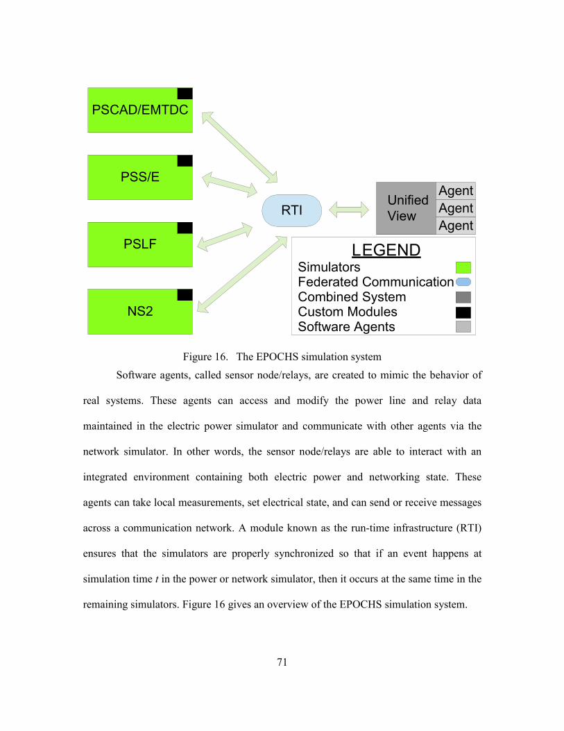
71
Figure 16. The EPOCHS simulation system
Software agents, called sensor node/relays, are created to mimic the behavior of
real systems. These agents can access and modify the power line and relay data
maintained in the electric power simulator and communicate with other agents via the
network simulator. In other words, the sensor node/relays are able to interact with an
integrated environment containing both electric power and networking state. These
agents can take local measurements, set electrical state, and can send or receive messages
across a communication network. A module known as the run-time infrastructure (RTI)
ensures that the simulators are properly synchronized so that if an event happens at
simulation time t in the power or network simulator, then it occurs at the same time in the
remaining simulators. Figure 16 gives an overview of the EPOCHS simulation system.
PSCAD/EMTDC
PSS/E
PSLF
NS2
RTIUnifiedView
AgentAgentAgent
LEGENDSimulatorsFederated CommunicationCombined SystemCustom ModulesSoftware Agents

72
EPOCHS has been used in previous experiments to show how network
communication provided by a Utility Intranet, such as the smart grid, could be used to
enhance the capabilities of protection and control systems. These experiments include
past work looking at zone 3 backup protection relays augmented with networking
communication capabilities [68]. Experiments with EPOCHS are able to show the
promise and potential pitfalls of next-generation smart grid technology applied to electric
power grid protection and control systems.
4.7 Simulation scenarios
Two simulation scenarios are presented in this chapter. The first scenario
simulates a shorted power line in a SCADA power grid containing trusted and untrusted
sensor node/relays. The second scenario simulates a cyber attacker’s attempt to cause a
power outage by gaining remote access to a sensor node/relay. Both scenarios are
mitigated by the proposed reputation-based trust management system.
Both scenarios are based on the communication-based backup protection system,
which was described in section 4.5. A backup protection system (BPS) engages circuit
breakers to isolate power line faults when the primary protection systems fails or
becomes inoperable. Hence, our reputation-based trust management system BPS must not
interfere with the primary protection system. Figure 17 and Figure 18 are used to
illustrate that the primary protection system is not interfered with, but supported by the
reputation-based trust management system.

73
Figure 17. Scenario 1, primary protection system non-interference example
Figure 18. Shortest path problem for Figure 17
Figure 17 represents an electric power grid with 2 generators and 8 trusted sensor
node/relays. The “X” between sensor node/relays S5 and S6 represents a fault on the
power line between these two nodes. The high trust values at all the nodes indicated that
the primary protection system will mitigate the faulty line by opening the circuit breakers
located at nodes S5 and S6. The reputation-based trust management system uses the
power grid topology with the detected fault’s location and a transformation algorithm to
reason about which regional peers should trip in order to contain the fault. The peers are
chosen based on proximity to the fault, as one would expect, but are also chosen based on
the trustworthiness of the peers based on their interactive history. A trust management
framework can be created using network flows, shortest paths, and other fundamental
H
S1
H
S2
H
S3
H
S4
H
S5
H
S6
H
S7
H
S8
100 100 100 100 100 100 100 100TrustValues
High VoltageLine H = Trusted NodeL = Untrusted Node
Legend: = Sensor nodes/relays, = Power Generator, = Power Bus, = Line Fault
X
X
SuperSource
Legend: = Relay Nodes, = Left side Junction Node, = Right side Junction NodeL
L R
S1
S2
S3
S4
S5
S6
S7
S8
SuperSink
0 00
62
3
4
5
4
3
2
R

74
algorithms. In the case of this backup protection system, a graph is created, as shown in
Figure 18. This graph is solved using Dijkstra’s shortest path algorithm [69]. The shortest
path between the super source node and the super sink node, highlighted in blue,
indicates that the circuit breakers located at S5 and S6 should be used to clear the detected
fault. This result agrees with the result expected from the primary protection system
indicating that the reputation-based trust management system supports the primary
protection system. The details on how the graph is generated from a given power grid
topology with a detected line fault is explained in the following section. Recall that the
first test case scenario uses the backup protection system within a power grid network
with trusted and untrusted nodes. This is illustrated in Figure 19 and Figure 20.
Figure 19. Scenario 2 improved BPS example
Figure 20. Shortest path problem for Figure 19
H
S1
H
S2
H
S3
L
S4
L
S5
L
S6
H
S7
H
S8
100 100 100 10 10 40 100 100TrustValues
High VoltageLine H = Trusted NodeL = Untrusted Node
Legend: = Sensor nodes/relays, = Power Generator, = Power Bus, = Line Fault
X
X
SuperSource
Legend: = Relay Nodes, = Left side Junction Node, = Right side Junction NodeL
L R
S1
S2
S3
S4
S5
S6
S7
S8
SuperSink
0 00
63.5
3
4
5
4
12
11
R

75
Figure 19 represents the same power grid topology with the same detected power
line fault between nodes S5 and S6 as in Figure 17. The difference between these two
figures is the nodes assigned trust values. In Figure 19, nodes S4, S5 and S6 are untrusted
with trust values of 10%, 10% and 40%, respectively. These lower trust values
correspond with the higher edge costs in Figure 20. This causes Dijkstra’s algorithm to
select a different path from the super source node to the super sink node. This updated
path is highlighted in blue in Figure 20 and indicates that the circuit breakers at locations
S3 and S7 should be engaged to clear the fault. These two nodes, S3 and S7, are the
closest trusted nodes to the detected fault. The selection of these two nodes by the backup
protection system minimizes the affected service area and the associated damages in
terms of financial costs. Notice that engaging the circuit breakers at S2 and S8 will also
mitigate the detected fault, but increase the size of the affected service area. The details
on how the graphs solved by Dijkstra’s algorithm are generated from a given power grid
topology with a detected line fault is explained in the following section.
The second scenario is included to emphasize the reasoning behind the proposed
reputation-based trust management system, which is to protect the smart grid enabled
power production and distribution system from cyber attacks. This goal is accomplished
by the trust management system’s implementation. The trust management system does
not engage any circuit breakers based on one sensor node/relay’s input. This
implementation requires, as a minimum, the inputs from two nodes and confirming
results from Dijkstra’s shortest path algorithm [69]. Hence, a cyber attacker gaining
access to one sensor node/relay cannot cause a power outage. The attacker would need to

76
gain access to at least 3 sensor node/relays to circumvent the proposed reputation-based
trust management system. These three nodes include: 1) the two nodes detecting the fault
and 2) a third node to assign trust values. These trust values are used by the
transformation algorithm to create the graph solved by Dijkstra’s algorithm [69].
4.8 Creating a graph to solve using the Dijkstra’s shortest path algorithm
Creating the shortest path problem in the backup protection relay’s trust
management system requires 1) knowledge of the power grid topology, 2) knowledge of
all sensor node/relays’ assigned trust values, and 3) knowledge of the location of the
detected line fault. The first requirement, “knowledge of the power grid topology,” would
need to be provided by SCADA system operators or a network discovery program. This
information is fairly static and only needs to be updated when changes occur.
The second requirement, “knowledge of all sensor node/relays’ assigned trust
values,” is provided using our previously developed simple trust algorithm as described
in chapter 2 and [30]. This algorithm assigns individual trust values to sensor node/relays
based on their sensor readings. This simple trust algorithm is a reputation based
algorithm, where nodes develop a reputation over time. This reputation is accomplished
by maintaining the trust history of the nodes and using this history to calculate each
node’s trust value. These calculated trust values represent the weighted sum of the nodes
historical trust values. These calculated trust values, τj, are used in Equation 37 below to
calculate an edge’s capacity. This trust value is updated on a recurring basis. The

77
simulations in this chapter used a 2 millisecond (ms) time-step, resulting in a 2 ms trust
value refresh rate.
The third requirement, “knowledge of the location of the detected line fault,” is
only needed when a fault occurs, i.e., when the primary protection system or backup
protection system must mitigate the problem. This line fault is detected by electronic
distance relays, which monitor the line impedance for out of tolerance changes. For
example, a high impedance measurement indicates an open power line and a low
impedance measurement indicates a shorted power line. The location of the line fault is
determined by the distance relays and provided to the graph generating algorithm.
Once the power grid topology is provided and trust values are established for the
relays in the system via the Simple Trust algorithm as describe in chapter 2 and in [30], a
method needs to be found to balance considerations of distance versus trust. This balance
needs to be set by the operators of the system since some may value the trade-off
differently than others. This is accomplished by adding two weighting variables α and β.
These two variables are inversely related to each other, which means one variable could
replace the other, such as, α=100/β. The decision to maintain two variable is intended to
clarify their functions and meaning within this algorithm. The α variable is the weighting
factor for distance from the detected fault location and β is the weighting factor for trust.
The weighted trust values combined with the weighted breakers' distance from the faults
is used to quantify a fault's associated damage area. Minimizing a fault's damage area
should minimize the total effect of the fault. The only remaining question is how to
combine these two values—trust values and distance from fault. The goal here is to

78
minimize the trip area by engaging trusted circuit breakers that are near the fault.
Minimizing the following objective function achieves this goal:
Minimize: ��𝑢�𝑛𝑖 ,𝑛𝑗�ℎ�𝑛𝑖 ,𝑛𝑗�|𝑁�|
𝑗=1
|𝑁�|
𝑖=1
(33)
Subject to: �ℎ�𝑛𝑖, 𝑛𝑗�|𝑁�|
𝑗=1
−�ℎ(𝑛𝑘,𝑛𝑖)|𝑁�|
𝑘=1
= �1 𝑖𝑓 𝑛𝑖 = 𝑆𝑜𝑢𝑟𝑐𝑒0 𝑖𝑓 𝑛𝑖 ≠ 𝑆𝑜𝑢𝑟𝑐𝑒 ∧ 𝑛𝑖 ≠ 𝑆𝑖𝑛𝑘
−1 𝑖𝑓 𝑛𝑖 = 𝑆𝑖𝑛𝑘�
(also known as Conservation Constraints)
(34)
ℎ�𝑛𝑖 ,𝑛𝑗� ≥ 0 𝑓𝑜𝑟 𝑎𝑙𝑙 𝑖, 𝑗 ∈ �1,2 … �𝑁��� (35)
𝑢�𝑛𝑖, 𝑛𝑗� = 0 𝑖𝑓 ⟨𝑛𝑖, 𝑛𝑗⟩ ∉ 𝐸� or 𝑛𝑗 ∉ 𝑁 (36)
𝑢�𝑛𝑖, 𝑛𝑗� = 𝛼 ⋅ ℎ𝑗 + 𝛽 ⋅ �1𝜏𝑗� 𝑖𝑓 𝑛𝑗 ∈ 𝑁 (37)
where
𝑁 the set of sensor node/relays in the SCADA network
𝑁� the set of nodes in the graph generated by Algorithm 1 and Algorithm 2
𝐸� the set of edges in the graph generated by Algorithm 1 and Algorithm 2
𝑖, 𝑗 ∈ �1,2, … |𝑁| … �𝑁��� are index variables used to enumerate the nodes in the graph generated by Algorithm 1 and Algorithm 2
ℎ𝑗 ∈ {𝑥|𝑥 ∈ ℕ ∧ 𝑥 ≤ ℎ𝑚𝑎𝑥 ∧ 𝑗 ≤ |𝑁|} the number of hops node 𝑗 is away from the fault, ℎ𝑚𝑎𝑥 is predetermined upper bound

79
𝜏𝑗 ∈ {𝑥|𝑥 ∈ ℚ ∧ 0 ≤ 𝑥 ≤ 1 ∧ 𝑗 ≤ |𝑁|} the trust value assigned to node 𝑗
𝛼 ∈ ℚ weighting factor, used to control the importance of distance
𝛽 ∈ ℚ weighting factor, used to control the importance of trust
𝑢:𝐸� → ℝ is a function mapping arcs to real values and represent the edge’s capacity
ℎ�𝑛𝑖 ,𝑛𝑗� ∈ {0,1} a binary variable used to determine if edge ⟨𝑛𝑖 ,𝑛𝑗⟩ is selected, i.e. along the shortest path
With ℕ, ℚ, and ℝ representing the set of natural, rational, and real numbers; respectively.
The values of |𝑁|, 𝛼, 𝛽 and ℎ𝑚𝑎𝑥 are provided by the SCADA system operator.
The values of 𝜏𝑖 are determined by the trust management system; namely by the simple
trust algorithm described in chapter 2 and in [30]. The values of ℎ𝑗 are determined by a
breath first search (BFS) like algorithm with a given maximum depth or distance
constraint, ℎ𝑚𝑎𝑥. The problem is how to determine which trusted sensor node/relay
circuit breakers to engage, i.e. the values of ℎ�𝑛𝑖 ,𝑛𝑗�. The binary variable ℎ�𝑛𝑖, 𝑛𝑗� is
used to select the trusted sensor node/relay circuit breakers to engage, i.e., a value of '1'
indicates that the corresponding sensor node/relay’s circuit breaker is selected and a value
of '0' indicates that the corresponding sensor node/relay is not selected. A graph generator
(Algorithms 1 and 2 below) converts the sensor node/relay power grid connectivity
topology to a graph, which is solved using Dijkstra’s shortest path algorithm [69]. The
nodes along the shortest path have their ℎ�𝑛𝑖 ,𝑛𝑗� binary variables set to '1', otherwise
zero.

80
The algorithm used to select trusted sensor node/relay circuit breakers to open
must be efficient in order to isolate/clear a detected SCADA error/fault within SCADA
timing constraints. This efficiency is quantified in terms of an algorithm’s order of
asymptotic growth notation, e.g., 𝑂 ��𝑁��2�, 𝑂 ���𝑁�� + �𝐸��� ∗ log�𝑁���, … etc. Dijkstra’s
shortest path algorithm [69], with a 𝑂 ���𝑁�� + �𝐸��� ∗ log�𝑁��� order of growth [70] may
be the best option—given the SCADA power grid topology transformation technique.
This symbol |𝑁| represents the number of nodes in a given SCADA network, 𝐺, and |𝐸|
represents the number of edges in 𝐺. The graph generated by Algorithm 1 and
Algorithm 2, 𝐺�, uses �𝑁�� and �𝐸�� for the number of nodes and edges in 𝐺�. The
transformation technique takes the input SCADA power grid network in Figure 19 and
generates the graph in Figure 20. The edge cost for the edges going in to the sensor
node/relays are calculated using 𝛼 ∗ ℎ𝑖 + 𝛽 ∗ �1𝜏𝑖�, with 𝛼 = 1, 𝛽 = 100, ℎ𝑚𝑎𝑥 = 10, 𝜏𝑖
trust values and ℎ𝑖 number of hops from the fault are provided by Figure 19. The edges
going into the Left Junction, Right Junction and Super Sink nodes are assigned a cost of
0. Dijkstra’s algorithm [69] determines the shortest path from the super source node to
the super sink node. That is, Dijkstra’s shortest path algorithm [69] assigns each edge in
𝐺� a '1' if it is along the shortest path between the super source node and the super sink
node, or '0' otherwise. In this case the shortest path between the super source and the
super sink traverses through 𝑆3 and 𝑆7. This indicates that tripping the breakers at 𝑆3 and
𝑆7 would have the greatest probability of isolating the fault, while minimizing the
affected damage area. The transformation algorithms are as follows:

81
Algorithm 1 SCADA_TMS_Transformation Pseudocode (N, E, F) 1. Procedure SCADA_TMS_Transformation // Inputs: 𝑁 is the set of SCADA nodes within the SCADA Power Grid, see Figure 19 // 𝐸 is the set of SCADA edges within the SCADA Power Grid, see Figure 19 // 𝐹 is the SCADA edge experiencing a Fault, i.e. 𝐹 ∈ 𝐸. // Note: Each edge is represented by a set of two nodes, i.e., 𝑒 ∈ 𝐸, 𝑒 = {𝑙𝑒𝑓𝑡, 𝑟𝑖𝑔ℎ𝑡}, // where 𝑙𝑒𝑓𝑡, 𝑟𝑖𝑔ℎ𝑡 ∈ 𝑁 and accessed by 𝑒. 𝑙𝑒𝑓𝑡 = 𝑙𝑒𝑓𝑡 and 𝑒. 𝑟𝑖𝑔ℎ𝑡 = 𝑟𝑖𝑔ℎ𝑡. 2. Begin // Initialization 3. 𝑁� ← ∅, 𝐸� ← ∅ // clear return variables--Node and Edge sets 4. 𝐿𝑒𝑓𝑡𝑟𝑜𝑜𝑡 ← 𝐹. 𝑙𝑒𝑓𝑡, 𝑅𝑖𝑔ℎ𝑡𝑟𝑜𝑜𝑡 ← 𝐹. 𝑟𝑖𝑔ℎ𝑡 // get fault end nodes, both left and right 5. 𝐸 ← 𝐸 − 𝐹 // remove fault edge from given set of Edges 6. 𝑁 ← 𝑁 − 𝐿𝑒𝑓𝑡𝑟𝑜𝑜𝑡 // remove left root node from given set of Nodes 7. 𝑁 ← 𝑁 − 𝑅𝑖𝑔ℎ𝑡𝑟𝑜𝑜𝑡 // remove right root node from given set of Nodes 8. ℎ ← 1, // set hop count value to 1 9. ℎ𝑚𝑎𝑥 ← 10 // set max hop value to 10 10. 𝛼 ← 1 // set hop distance weighting factor to 1 11. 𝛽 ← 100 // set trust weighting factor to 100 // Add Super Source, Left Junction, Right Junction and Super Sink Nodes to // return variables, 𝑁� 𝑎𝑛𝑑 𝐸�—see Figure 20 12. 𝑁� ← 𝑁� ∪ {𝑆} ∪ {𝐿} ∪ {𝑅} ∪ {𝑇} 13. 𝐸� ← 𝐸� ∪ �{𝑆, 𝐿, 𝑐𝑜𝑠𝑡 ← 0}�
14. 𝐸� ← 𝐸� ∪ ��𝐿, 𝐿𝑒𝑓𝑡𝑟𝑜𝑜𝑡 , 𝑐𝑜𝑠𝑡 ← 𝛼 ∗ ℎ + 𝛽 ∗ � 1𝐿𝑒𝑓𝑡𝑟𝑜𝑜𝑡.𝑡𝑟𝑢𝑠𝑡
��� ∪ �{𝐿𝑒𝑓𝑡𝑟𝑜𝑜𝑡 ,𝑅, 𝑐𝑜𝑠𝑡 ← 0}�
// Call recursive helper function for left side nodes 15. Build_Graph�𝑁,𝐸,𝑁�,𝐸� , 𝐿𝑒𝑓𝑡𝑟𝑜𝑜𝑡 , 𝐿,𝑅, ℎ, ℎ𝑚𝑎𝑥�
16. 𝐸� ← 𝐸� ∪ ��𝑅,𝑅𝑖𝑔ℎ𝑡𝑟𝑜𝑜𝑡 , 𝑐𝑜𝑠𝑡 ← 𝛼 ∗ ℎ + 𝛽 ∗ � 1𝑅𝑖𝑔ℎ𝑡𝑟𝑜𝑜𝑡.𝑡𝑟𝑢𝑠𝑡
��� ∪ �{𝑅𝑖𝑔ℎ𝑡𝑟𝑜𝑜𝑡 ,𝑇, 𝑐𝑜𝑠𝑡 ← 0}�
// Call recursive helper function for right side nodes 17. Build_Graph�𝑁,𝐸,𝑁�,𝐸� ,𝑅𝑖𝑔ℎ𝑡𝑟𝑜𝑜𝑡 ,𝑅,𝑇, ℎ, ℎ𝑚𝑎𝑥� 18. Return 𝑁�,𝐸� 19. End procedure SCADA_TMS_Transformation Note: This algorithm uses a SCADA power grid connectivity graph (N, E) and a
fault location edge (F) to construct a graph problem, solvable by Dijkstra’s shortest path algorithm [69].

82
Algorithm 2 Build_Graph Pseudocode �𝑁,𝐸,𝑁�,𝐸� , 𝑟𝑜𝑜𝑡, 𝑗,Ω, h, hmax� 1. Procedure Build_Graph // Inputs: 𝑁 is the set of SCADA nodes within the SCADA Power Grid, see Figure 19 // 𝐸 is the set of SCADA edges within the SCADA Power Grid, see Figure 19 // 𝑁� is the set of network flow problem nodes // 𝐸� is the set of network flow problem edges // 𝑟𝑜𝑜𝑡 is the starting node in 𝑁 // 𝑗 is the source node in 𝑁� // Ω is the end node in 𝑁� // ℎ𝑚𝑎𝑥 is the maximum allowed hop distance from the fault // Note: all above variables are passed by reference // ℎ is the hop distance from the fault 2. Begin // Check Exit conditions 3. If (𝐸 == ∅) or (𝑁 == ∅) or (ℎ ≥ ℎ𝑚𝑎𝑥) 4. Return 5. End If // Initialization 6. 𝑡𝑒𝑚𝑝_𝑒𝑑𝑔𝑒𝑠 ← ∅, 𝑡𝑒𝑚𝑝_𝑛𝑜𝑑𝑒𝑠 ← ∅, ℎ ← ℎ + 1, 𝛼 ← 1, 𝛽 ← 100 // find all nodes adjacent to 𝑟𝑜𝑜𝑡 in 𝑁 7. For each 𝑒 in 𝐸 8. If (𝑒. 𝑙𝑒𝑓𝑡 == 𝑟𝑜𝑜𝑡) and (𝑒. 𝑟𝑖𝑔ℎ𝑡 ∈ 𝑁) 9. 𝑡𝑒𝑚𝑝_𝑒𝑑𝑔𝑒𝑠 ← 𝑡𝑒𝑚𝑝_𝑒𝑑𝑔𝑒𝑠 ∪ 𝑒 10. 𝑡𝑒𝑚𝑝_𝑛𝑜𝑑𝑒𝑠 ← 𝑡𝑒𝑚𝑝_𝑛𝑜𝑑𝑒𝑠 ∪ 𝑒. 𝑟𝑖𝑔ℎ𝑡 11. End If 12. If (𝑒. 𝑟𝑖𝑔ℎ𝑡 == 𝑟𝑜𝑜𝑡) and (𝑒. 𝑙𝑒𝑓𝑡 ∈ 𝑁) 13. 𝑡𝑒𝑚𝑝_𝑒𝑑𝑔𝑒𝑠 ← 𝑡𝑒𝑚𝑝_𝑒𝑑𝑔𝑒𝑠 ∪ 𝑒 14. 𝑡𝑒𝑚𝑝_𝑛𝑜𝑑𝑒𝑠 ← 𝑡𝑒𝑚𝑝_𝑛𝑜𝑑𝑒𝑠 ∪ 𝑒. 𝑙𝑒𝑓𝑡 15. End If 16. End For each // Update the given nodes and edges 17. 𝐸 ← 𝐸 − 𝑡𝑒𝑚𝑝_𝑒𝑑𝑔𝑒𝑠 18. 𝑁 ← 𝑁 − 𝑡𝑒𝑚𝑝_𝑛𝑜𝑑𝑒𝑠 19. If (𝑡𝑒𝑚𝑝_𝑒𝑑𝑔𝑒𝑠 == ∅) or (𝑡𝑒𝑚𝑝_𝑛𝑜𝑑𝑒𝑠 == ∅) 20. Return 21. End If 22. If (|𝑡𝑒𝑚𝑝_𝑛𝑜𝑑𝑒𝑠| == 1) 23. 𝑁� ← 𝑁� ∪ 𝑡𝑒𝑚𝑝_𝑛𝑜𝑑𝑒𝑠
24. 𝐸� ← 𝐸� ∪ ��𝑗, 𝑡𝑒𝑚𝑝_𝑛𝑜𝑑𝑒𝑠. 𝑒𝑙𝑒𝑚𝑒𝑛𝑡, 𝑐𝑜𝑠𝑡 ← 𝛼 ∗ ℎ + 𝛽 ∗ 1𝑡𝑒𝑚𝑝_𝑛𝑜𝑑𝑒𝑠.𝑒𝑙𝑒𝑚𝑒𝑛𝑡.𝑡𝑟𝑢𝑠𝑡
��
25. 𝐸� ← 𝐸� ∪ {{𝑡𝑒𝑚𝑝_𝑛𝑜𝑑𝑒𝑠. 𝑒𝑙𝑒𝑚𝑒𝑛𝑡,Ω, cost ← 0}} 26. Build_Graph�𝑁,𝐸,𝑁�,𝐸� , 𝑡𝑒𝑚𝑝_𝑛𝑜𝑑𝑒𝑠. 𝑒𝑙𝑒𝑚𝑒𝑛𝑡, 𝑗,Ω, ℎ, ℎ𝑚𝑎𝑥� 27. Return 28. End If // spit point found requiring addition virtual junction nodes 29. 𝐽𝑢𝑛𝑐𝑡𝑖𝑜𝑛𝑖𝑛 ← 𝑛𝑒𝑤 𝑣𝑖𝑟𝑡𝑢𝑎𝑙 𝐽𝑢𝑛𝑐𝑡𝑖𝑜𝑛 𝑛𝑜𝑑𝑒 30. 𝑁� ← 𝑁� ∪ {𝑗𝑢𝑛𝑐𝑡𝑖𝑜𝑛𝑖𝑛} 31. 𝐸� ← 𝐸� ∪ {{𝑗, 𝑗𝑢𝑛𝑐𝑡𝑖𝑜𝑛𝑖𝑛, 𝑐𝑜𝑠𝑡 ← 0}} 32. For each 𝑛𝑜𝑑𝑒 in 𝑇𝑒𝑚𝑝_𝑛𝑜𝑑𝑒𝑠 33. 𝑗𝑢𝑛𝑐𝑡𝑖𝑜𝑛𝑜𝑢𝑡 ← 𝑛𝑒𝑤 𝑣𝑖𝑟𝑡𝑢𝑎𝑙 𝑗𝑢𝑛𝑐𝑡𝑖𝑜𝑛 𝑛𝑜𝑑𝑒

83
34. 𝑁� ← 𝑁� ∪ {𝑗𝑢𝑛𝑐𝑡𝑖𝑜𝑛𝑜𝑢𝑡} 35. Build_Graph�𝑁,𝐸,𝑁�,𝐸� ,𝑛𝑜𝑑𝑒, 𝑗𝑢𝑛𝑐𝑡𝑖𝑜𝑛𝑖𝑛 , 𝑗𝑢𝑛𝑐𝑡𝑖𝑜𝑛𝑜𝑢𝑡 , ℎ, ℎ𝑚𝑎𝑥� 36. 𝑗𝑢𝑛𝑐𝑡𝑖𝑜𝑛𝑖𝑛 ← 𝑗𝑢𝑛𝑐𝑡𝑖𝑜𝑛𝑜𝑢𝑡 37. End For each 38. 𝐸� ← 𝐸� ∪ {{𝑗𝑢𝑛𝑐𝑡𝑖𝑜𝑛𝑜𝑢𝑡 ,Ω, cost ← 0}} 39. Return 40. End procedure Build_Graph
4.9 Results
The proposed reputation-based trust management system does not interfere with
the primary protection system, provides protection against cyber attacks that are
detectable through reputation-based trust, and improves the backup protection scheme
with a much better response time (50 ms) than traditional SCADA backup protection
schemes (~1.5 seconds), see Figure 21 and Figure 22. This last benefit is due to the
additional shared knowledge available in a smart grid enabled power grid. The traditional
power grid backup protection schemes utilized pilot wires, timeout timers, and point to
point communication lines. These results help to illustrate some of the strong benefits
provided by context-aware smart protection schemes. These experiments provide an
indication that the employment of a trust management system can help to mitigate some
of the security concerns in using smart grid enabled protection and control systems.
Figure 21. Faulty line isolated within 50 ms with the TMS
-4-202468
0 0.2 0.4 0.6 0.8 1 1.2 1.4 1.6 1.8 2
Phas
e A
Curr
ent
(Kilo
-Am
pere
s)
Simulation Time (Seconds)

84
Figure 22. Faulty line isolated within ~1.5 seconds [45] without the TMS
4.10 Summary
Smart grid technology, where network communication is used to provide far
greater context-awareness than is currently available, has the potential to make many
advances in protection and control systems in the electric power grid. At the same time,
Internet based network communication capabilities introduce new vulnerabilities which
need to be addressed. The proposed reputation-based trust management system has
shown promise, in the communication-based backup protection system simulated in this
chapter, to work comparably to systems without the trust management system when no
attacks or other failures occur and to operate effectively even when some elements in the
system are compromised by attacks or from accidental breakdowns. The results show
promise of similar benefits in other smart communication-based protection and control
systems.
-4-202468
0 0.2 0.4 0.6 0.8 1 1.2 1.4 1.6 1.8 2
Phas
e A
Curr
ent
(Kilo
-Am
pere
s)
Simulation Time (Seconds)

85
V. A Trust Management Toolkit for Smart Grid Protection Systems∗
5.1 Chapter Overview
This section develops the trust management toolkit and proposes its use in future
smart grid protection systems. This solution is a robust and configurable trust
management toolkit protection system augmentation, which can successfully function in
the presence of untrusted (malfunctioning or malicious) smart grid protection system
nodes. The trust management toolkit combines reputation-based trust with network flow
algorithms to identify and mitigate faulty smart grid protection system components. This
trust management toolkit assigns trust values to all smart grid protection system
components. Faulty components, attributed to malfunctions or malicious cyber attacks,
are assigned a lower trust value, which indicates a higher risk of failure. The utility of this
trust management toolkit is validated through experiments comparing the trust
management toolkit modified backup and special protection systems to the original
backup and special protection systems via an ANOVA analysis. These simulation results
show promise concerning the effectiveness of the trust management toolkit.
5.2 Introduction
Smart grid enabled technologies are expected to improve the reliability and
efficiency of the world’s electric power grids [51]. This technology is needed to help
mitigate growing energy demands, which is attributed, in part, to increased population
∗ [71] J. E. Fadul, K. M. Hopkinson, T. R. Andel, and J. T. Moore, "A Trust Management Toolkit for Smart Grid Protection Systems," IEEE Transactions on Smart Grid, p. Submitted for publication, 2011.

86
size [72, 73] and technological advancements [6]. Although definitions vary, the term
“smart grid” often refers to the use of digital equipment that employs network
communication to enable a greater situational awareness for protection, control, and other
core power grid mechanisms, than is possible with traditional power grid equipment. This
is the definition of smart grid technology used in this section. The improved situational
awareness enables enhanced operational efficiency and reliability. The use of smart grid
technology makes it possible to improve legacy protection systems, which currently
mitigates detected faults with predetermined actions, by taking advantage of greater
cooperation and sharing of information between protection system components. The
legacy protection system’s approach is appropriate for the previously limited context
aware power grid environment. The increased bandwidth in future smart grids will
improve the systems’ context awareness and enable better protection system decisions
concerning faults in dynamic power grid environments. The trust management toolkit
developed in this section modifies legacy protection components to better utilize the
increased bandwidth capacity in smart grids and improve decision making processes in
the presence of failures, disruptions, and malicious behavior.
The trust management toolkit has three major modules; a trust assignment
module, a fault detection module, and a decision module. The trust assignment module
uses context sensitive information and periodic intercommunication messages to
determine individual smart grid protection components’ trust values. The fault detection
module uses trip signals generated by traditional distance relays and frequency
disturbance monitoring devices to detect line and system faults, respectively. The

87
decision module combines and analyzes the current power grid conditions; the detected
fault conditions and the protection components’ assigned trust values, to decide on the
most reliable corrective action, where reliable means minimal risk of failure to mitigate
the detected fault condition. Software simulations have demonstrated the potential
benefits of the trust management toolkit in backup and special protection system test case
scenarios.
The trust management toolkit augmented backup and special protection system
test case scenarios utilized the electric power and communication synchronizing
simulator (EPOCHS) [68] simulation platform. EPOCHS is a simulation environment
that federates, or combines, Network Simulator 2 (NS2) [32], the Power Systems
Computer Aided Design (PSCAD) [66], and the Power System Simulation for
Engineering (PSS/E) [65]. NS2 [32] is an open source network simulation developed for
academic and research uses. PSCAD [66] and PSSE [65] are commercial electromagnetic
and electromechanical power system transient simulators, respectively. EPOCHS [68] is
a middleware platform used to coordinated and control the interactions between NS2 [32]
and the commercial power simulators. The resulting raw simulation data is analyzed with
the open source R statistical package [74]. An analysis of variance (ANOVA) and a
comparison of confidence intervals (CI) [46] is used to determine the statistical
significance of the simulation results.
Simulation results support the use of the proposed trust management toolkit, or a
similar toolkit, in backup and special protection systems operated within a smart grid
environment among untrusted protection system nodes. This will result in equal (if not

88
improved) speed and accuracy when compared to traditional systems. The utility of this
trust management toolkit is validated through experiments comparing the trust
management toolkit modified backup and special protection systems to the original
backup and special protection systems and their associated ANOVA analysis. The main
contribution of this paper is a robust and configurable trust management toolkit
protection system augmentation, which can successfully function in the presence of
untrusted (malfunctioning or malicious) smart grid protection system nodes. This trust
management toolkit should be included in future smart grid implementations.
This section is divided into seven subsections. Subsection 5.2 is the introduction.
Section 5.3 provides background and related work information. Section 5.4 describes the
trust management toolkit’s implementation and its use to augment previously published
backup and special protection systems. Section 5.5 covers the testing environment used in
this section’s simulations and the procedure used to compare the augmented protection
systems to their original versions. Section 5.6 presents the experimental results and
discusses their statistical and real world significance. Section 5.7 contains this Section’s
conclusion.
5.3 Background and Related Work
5.3.1 Background
In the United States, the nation’s electric power grid has been deemed a matter of
national security by the previous two presidents [7-11, 75] and the current
administration [12]. This was further supported by the codification of the Energy
Independence and Security Act (EISA) of 2007 [51] Title XIII sections 1301—1306,

89
Smart Grid. EISA of 2007 [51] Title XIII, section 1301 identifies ten characteristics of a
smart grid, whose intent is to modernize the electric power grid and enable it to safely
operate closer to its peak capacity. The proposed trust management toolkit supports seven
of these ten characteristics. For example, the trust management toolkit supports the first
characteristic; namely, increased use of digital information and controls technology to
improve reliability, security, and efficiency of the electric grid, by using context sensitive
information to improve the decision making process.
The proposed trust management toolkit is enabled by a smart grid’s increased
communications bandwidth and its implementation of standard Internet protocols and
associated technologies. Other smart grid enabled technologies include microgrids [20]
and demand response [19], which should help reduce the current and future projected
increases in energy demands on the U.S. power grid. Microgrid technologies [20] refers
to small power grids with local producers of energy, such as wind mills or solar panels,
which draw little to no energy from the nation's power grid in order to supply their local
customers. Demand response [19] advanced metering infrastructure attempts to optimize
the power grid’s efficiency by enabling the average consumer to automatically control
how much energy they draw, from the electric power grid, based on current energy costs
and energy demands. The trust management toolkit uses demand response information in
determining the best response to a detected error condition and may use microgrid
technologies information in future implementations.
Power grid protection systems are used to mitigate detected faults and minimize
their impact on customers. Two of these protection schemes are backup and special

90
protection systems. Backup protection system assemblies are tasked with clearing faults
when primary protection assemblies fail or become inoperable [28]. The trust
management toolkit improves the backup protection system’s response time by utilizing
context sensitive trust information in the selection of relays to engage and clear the fault.
Special protection systems [29] monitor one or more power grid systems for error
conditions and take predetermined corrective actions to mitigate the detected error
conditions. In this paper, the trust management toolkit augmented special protection
system test cases monitor system frequency for error conditions and dynamically select
the corrective action with the highest probability of successfully mitigating the detected
error conditions. The trust management toolkit enhanced backup and special protection
system test case scenarios are further discussed in subsection 5.5.
The trust management toolkit uses network flow techniques [26, 54, 57, 58],
problem formulations [27], and solution algorithms [55, 56, 69] in the trust assignment
and decision modules. Here the term network represents a set of nodes and edges and the
term flow represents a path between two specific nodes. Network flow techniques
encompass the idea of optimizing an objective function, while insuring flow conservation
along non-negative capacitated edges. The maximum flow problem formulations
algorithms used are image segmentation [27] and image labeling [27]. Both of these
algorithms utilized the maximum flow / minimum cutset duality in segregating the
network nodes into trusted and untrusted sets. The solution algorithms used are Dijkstra’s
shortest path algorithm [69] and a modified version of Goldberg’s HIgh-level Push-
Relabel flow (HIPR) algorithm [55]. The modification to HIPR [55] incorporates the

91
Curet et al. [56] algorithm for finding all minimum cutsets in a given network flow
problem. An explanation of the trust management toolkit’s implementation of these
network flow techniques is provided in subsection 5.4.
5.3.2 Trust Management Related Work
The previous efforts of Marsh [53], Buchegger et al. [42], Zimmermann [40],
Blaze et al. [39], Housley et al. [41], Kamvar et al. [43], Hopkinson et al. [68],
Wang et al. [45], and Igure et al. [44] provided guidance on how to define trust in a smart
grid network. David Marsh [53] was one of the first authors to formally define and assign
trust values to software agents’ interactions. Matt Blaze et al. [39] coined the term “Trust
Management Problem.” This term refers to the framework used to study security policies,
security credentials and trusted relationships. Matt Blaze et al. [39] work resulted in two
software programs (PolicyMaker and Keynote), which utilize Pretty Good Privacy
(PGP) [40] and X.509 [41] for individual authentication across a computer network.
CONFIDANT [42] and EigenTrust [43] protocols served as inspiration for the
initial incarnation of the trust management toolkit (i.e., Simple Trust protocol [30]). Also,
the preliminary work by Hopkinson et al. [68], Wang et al. [45], and Igure et al. [44],
where agents within Supervisory Control and Data Acquisition (SCADA) systems were
shown (via computer simulation) to be viable cyber security preventative options.
Furthermore, the agent-based SCADA trust system developed by Borowski et al. [76]
supports the idea of a backup protection system augmented by a trust system, which is
expanded upon in the proposed trust management toolkit.

92
5.4 Trust Management Toolkit
The trust management toolkit uses network flow techniques and reputation-based
trust values to improve smart grid protection system fault response times and resiliency to
intentional and unintentional protection component and communication network errors.
Intentional errors are malicious acts by rogue individuals or organizations, intent on
exploiting the need for electricity, for political or financial gains. Unintentional errors are
component failures due to normal wear and tear, manufacturing defects, or non-malicious
maladjustments of settings, i.e., operator or technician errors. The trust management
toolkit is composed of three modules, namely; a trust assignment module, a fault
detection module and a decision module. The implementation of these three modules is
discussed next.
5.4.1 Trust Assignment Module
The trust assignment module develops and assigns trust values to smart grid
protection components, where trust is the probability that a component will function
correctly when tasked to perform some action. This module uses context sensitive
information to develop initial reputation based trust values. These initial trust values are
processed using network flow techniques to mitigate false trust levels. In this case, a false
positive is a non-malicious trust agent assigned a low trust value and a false negative is a
malicious trust agent assigned a high trust value. These trust values are used by the
decision module in selecting the best response to a detected fault condition.
The context sensitive information shared by smart grid protection components are
line conditions (e.g., voltages, currents and impedances) for the trust management toolkit

93
enhanced backup protection system and system conditions (e.g., generator frequencies)
for the trust management toolkit enhanced special protection system. This shared
information is used to reach a consensus concerning the state of the line or the system.
The protection components in agreement with the consensus are assigned an initial high
trust value and those whom disagree are assigned an initial low trust value. These initial
trust values are filtered to identify and correct false positive and false negative trust
values using image segmentation [27] or image labeling [27] algorithms.
Image segmentation [27] and image labeling [27] are algorithms used to
formulate maximal network flow problems. The maximal flow from an artificial super
source node to an artificial super sink node is determined using HIPR [55]. The
corresponding minimum cutset is used to partition the protection component nodes into
sets with varying levels of trust. Figure 23, is a small pedagogical example of image
segmentation [27]. The super source and sink nodes are displayed as boxes and circles
represent the two protection nodes (S1 and S2). The non-negative edge values represent
the probability that a protection component node is trusted (a1 and a2), untrusted (b1 and
b2) and the penalty (p12 and p21) assessed for assigning different trust values to these two
nodes. In this example, S1 is on the Source side of the cut and assigned a high trust value,
while S2 is on the Sink side of the cut and assigned a low trust value. These assigned trust
values are used by the decision module in determining the best option for mitigating a
detected fault condition.

94
Figure 23. Image segmentation pedagogical example [48]
An image labeling pedagogical example is shown in Figure 24. The super source
(S) and super sink (T) nodes are displayed as boxes and the two protection nodes (S1 and
S2) are represented by sets of circles. Each protection node is represented by a set of five
circles. Each circle (Si,k) represents a level of trust, where i is the protection node’s
identification number and k is a level of trust. The non-negative edges ai,k, pi,j
55
and L
represent the likelihood of protection node i being assigned a trust level of k, the penalty
assessed for assigning protection nodes i and j different trust values and the return
capacity L included for completeness. In this example, S1 with four of its circles on the
source side of the cut is assigned a trust level of 4 and S2 with two of its circles on the
source side of the cut is assigned a trust level of 2. As with image segmentation, these
continually calculated trust values are determined using the HIPR [ ] algorithm to
partition the network into two sets, a trusted set of nodes and an untrusted set of nodes.
S1
S2
SuperSource
SuperSink
a1
a2
b1
b2
p12
p21
The Cut

95
Of course, these assigned trust values are used by the decision module in determining the
best option for mitigating a detected fault condition.
Figure 24. Image labeling pedagogical example [48]
5.4.2 Fault Detection Module
The fault detection module monitors one or more predetermined values for
changes that indicate a condition requiring corrective action. The predetermined values in
the PSCAD-based backup protection system test cases consist of line impedances via
distance relays and in PSSE-based special protection system test cases they include grid
frequencies measured at all generator and load locations. The trust management toolkit’s
decision module is notified when a monitored value exceeds or falls below its
predetermined limits.
5.4.3 Decision Module
The decision module uses the previously assigned trust values to validate the
detected fault and responds appropriately to minimize power grid downtime. The
S1,1 S1,3S1,2 S1,4 S1,5
S T
S2,1 S2,3S2,2 S2,4 S2,5
L
L L L L
L
LLLLL
La1,0
a1,1 a1,2 a1,3 a1,4
a1,5
a2,0 a2,1 a2,2 a2,3 a2,4a2,5
The Cut
p1,2 p1,2
p1,2
p1,2p1,2

96
decision module is a distributed piece of autonomous software that is capable of
independent analysis and actions. The decision module’s corrective actions are either
static or dynamic. The static actions are predetermined and scripted (such as with a truth
table [48] or flowchart [59]), while dynamic actions use context sensitive smart grid
information to minimize the effects of a validated fault on the power grid’s customers.
For example, the flowchart depicted in Figure 25 statically enforces the requirement for
two trusted smart grid protection node initiated trip signals before executing the trip
signal’s request and tripping a given line breaker. The dynamic actions are more difficult
and entail selecting the smallest number of protection system nodes with the highest
probability (also known as trust value) of successfully mitigating the detected fault with
minimal impact on the power grid’s customers. Two approaches for dynamically
determining corrective actions are discussed next; namely network flow and greedy
algorithm approaches.
The network flow approach used by the trust management toolkit in the PSCAD
test cases is an optimization approach where the objective function (38), is minimized
subject to the constraints given in (39)-(42). Minimizing the objective function (38)
represents the minimization of the sum between risk of failure and affected size of power
grid’s outage. Minimizing the risk of failure can also be thought of as maximizing the
probability of successfully mitigating the detected fault (i.e., maximizing the summed
trust values).
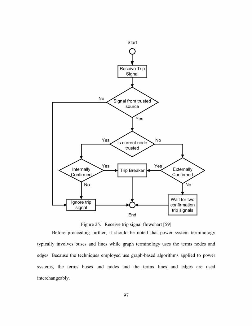
97
Figure 25. Receive trip signal flowchart [59]
Before proceeding further, it should be noted that power system terminology
typically involves buses and lines while graph terminology uses the terms nodes and
edges. Because the techniques employed use graph-based algorithms applied to power
systems, the terms buses and nodes and the terms lines and edges are used
interchangeably.
Start
Receive TripSignal
Signal from trustedsource
Ignore tripsignal
Is current nodetrusted
InternallyConfirmed
ExternallyConfirmed
Trip Breaker
Wait for twoconfirmationtrip signals
End
Yes
No
Yes No
Yes Yes
No No

98
Minimize: ��𝑢�𝑛𝑖 ,𝑛𝑗�ℎ�𝑛𝑖, 𝑛𝑗�|𝑁�|
𝑗=1
|𝑁�|
𝑖=1
(38)
Subject to:
�ℎ�𝑛𝑖 ,𝑛𝑗�|𝑁�|
𝑗=1
−�ℎ(𝑛𝑘,𝑛𝑖)|𝑁�|
𝑘=1
= �1 𝑖𝑓 𝑛𝑖 = 𝑆𝑜𝑢𝑟𝑐𝑒0 𝑖𝑓 𝑛𝑖 ≠ 𝑆𝑜𝑢𝑟𝑐𝑒 ∧ 𝑛𝑖 ≠ 𝑆𝑖𝑛𝑘
−1 𝑖𝑓 𝑛𝑖 = 𝑆𝑖𝑛𝑘�
(also known as Conservation Constraints)
(39)
ℎ�𝑛𝑖 ,𝑛𝑗� ≥ 0 𝑖, 𝑗 ∈ �1,2 … �𝑁��� (40)
𝑢�𝑛𝑖 ,𝑛𝑗� = 0 𝑖𝑓 ⟨𝑛𝑖, 𝑛𝑗⟩ ∉ 𝐸� or 𝑛𝑗 ∉ 𝑁 (41)
𝑢�𝑛𝑖, 𝑛𝑗� =
𝛼 ⋅ ℎ𝑗 + 𝛽 ⋅ �1𝜏𝑗�
𝑖𝑓 𝑛𝑗 ∈ 𝑁 (42)
Where
𝐸� is the set of edges in the constructed graph
�𝑁�� is the number of nodes in the constructed graph
𝑁 is the set of protection system nodes
|𝑁| is the number of protection node relays
𝑖, 𝑗 are index variables used to enumerate the sensor nodes/relays

99
ℎ𝑗 is the number of hops node j is away from the fault with a predetermine upper
bound of ℎ𝑚𝑎𝑥
𝜏𝑗 is the trust value assigned to sensor node/relay j
𝛼 weighting factor, used to control the importance of distance
𝛽 weighting factor, used to control the importance of trust
𝑢�𝑛𝑖 ,𝑛𝑗� function mapping edges ⟨𝑛𝑖 ,𝑛𝑗⟩ to their edge cost
ℎ�𝑛𝑖 ,𝑛𝑗� function mapping edges ⟨𝑛𝑖 ,𝑛𝑗⟩ to 1 if the edge is used within the shortest
path, otherwise 0.
The values of |N|, α, β and hmax are given by the smart grid system operator. The
values of τj are determined by the trust assignment module and the location of the
detected fault is provided by the fault detection module. The values of hj are determined
by a breadth first search like algorithm that starts from the given fault location with a
given maximum depth or distance constraint, hmax
Figure 28
. A recursive graph generator algorithm
transforms the power grid’s one line diagram (see ) into a graph (see Figure 29),
which is solved using Dijkstra’s shortest path algorithm [69]. Equation (38) is minimized
by the identified shortest path from the super source node to the super sink node. The
binary function ℎ�𝑛𝑖 ,𝑛𝑗� returns a '1' when protection system node 𝑛𝑗 is traversed along
the shortest path, otherwise zero. This binary function ℎ�𝑛𝑖,𝑛𝑗� also identifies the trusted
protection system node’s relay 𝑛𝑗 line breakers to engage, i.e., a value of '1' indicates that
the corresponding protection system node’s relay is engaged (opening the associated line

100
breaker) and a value of '0' indicates that the corresponding protection system node’s relay
is not engaged.
The greedy approach used by the trust management toolkit in the PSS/E-based
special protection system test cases uses a sorting algorithm to determine the order in
which the protection system nodes are selected for load shedding. This sorting algorithm
uses smart grid’s demand response data in conjunction with assigned trust values, node
type and load values to sort all the protection system nodes. Table 5 is an example of a
sorted set of such nodes. Notice that the nodes are sorted by the first four columns with
an order of precedence from left to right, i.e., first sort by Type and then by Trust Value
followed by Demand Response and lastly by Load (MW). The columns are type of
protection system, node’s trust value assigned, demand response participant (yes or no),
load amount at the node, customer authorized load shed amount (10% of load amount in
this example), and the node’s identification number. If a frequency disturbance is
detected and requires the power grid to shed 200 MW of power, then the greedy
algorithm would attempt to meet this requirement by selecting the first load node in
Table 5, namely node 120. If the selection of this first node is not enough to meet the
requirement, then the greedy algorithm would select the next node, namely node 73. Now
the selected nodes have enough load available for shedding (i.e., 330 MW) to meet the
requirement—enabling the greedy algorithm to stop selecting additional nodes for load
shedding. The trust management toolkit’s decision module uses the two selected nodes to
meet the load shedding requirement. Hence, the decision module is able to meet the load
shed requirement with minimal impact to power grid customers. If the load shed

101
requirement was greater than 330 MW, then the greedy algorithm would continue
selecting nodes until the requirement was met or the system operator intervened.
Table 5. Sorted Nodes for Possible Load Shedding
Type Trust Value
Demand Response
Load (MW)
Shed Amt (MW)
Node ID
Load High Yes 1812 181 120 Load High Yes 1492 149 73 Load High No 1492 149 25 Load High No 1250 125 72 Load Low No 1592 159 33 Load Low No 1492 149 82
5.4.4 Trust Management Toolkit Test Cases
The utility of the proposed trust management toolkit is demonstrated by computer
simulations of augmented backup and special protection systems within power grid test
cases. The protection systems are augmented as follows:
1) Trust Management Toolkit Augmented Backup Protection System
The traditional backup protection system is augmented with a trust management
toolkit. The assignment module utilizes current grid power line information in a
reputation based trust manor, with image segmentation and image labeling algorithms, to
establish and assign trust values. The fault detection module uses the traditional distance
relay mechanism to detect line faults. The decision module minimizes the objective
function (38) to determine which protection system relays to engage.
2) Trust Management Toolkit Augmented Special Protection System
The traditional special protection system is augmented with a trust management
toolkit. The assignment module utilizes current grid frequency information in a reputation

102
based trust manor to establish and assign trust values. The fault detection module uses the
traditional frequency disturbance mechanism to detect system conditions indicative of an
imminent under-frequency fault. The decision module uses a greedy algorithm approach
to determine which buses to select for load shedding.
5.5 Methodology
5.5.1 Testing Environment
The trust management toolkit demonstration test case scenarios make use of
EPOCHS [68], NS2 [32] (including NAM [47]), PSCAD [66] and PSS/E [65], where the
PSCAD [66] electromagnetic transient simulator is used for the backup protection system
test case scenarios and the PSS/E [65] electromechanical transient simulator is used for
the special protection system test case scenarios. NS2 [32] is the network simulator used
to represent the increased bandwidth in an Internet-like smart grid utility intranet. In
networking terms a smart grid is considered a wide area network servicing a utility’s
Regional Transmission Organization (RTO) region’s customers, see Figure 26. The smart
grid interconnects multiple node types; such as, control centers, power plants, substations
and customers (e.g., residential, commercial, industrial, medical and educational
institutions). Each node type may be represented by a software agent in NS2 [32], where
software agents are autonomous software entities designed to mimic the behavior of real
world systems. It is important to note that in a real world implementation of this trust
management toolkit, these software agents would reside inside Intelligent Electronic
Devices (IED) strategically located across the smart grid. In the simulation environment,
these software agents communicate with each other via NS2 [32] and with their

103
corresponding power simulator component via EPOCHS [68], see Figure 27. Each
software agent represents a single power simulator component, such as a load bus in
PSS/E [65] or a power bus in PSCAD [66]. Each software agent can access and modify
their corresponding power component’s data (e.g., access sensor data, engage relays,
change load power levels, etc). The software agents’ capabilities enable seamless
integration of the trust management toolkit modules with a simulated smart grid enhanced
power grid.
Figure 26. Abstract representation of a smart grid wide area network [68]
Figure 27. The EPOCHS simulation system [68]
Ethernet LAN
Host Computer
ProtectionIED
ProtectionIED
ControlIED
ControlIED
Smart Grid
Power PlantSubstation
Router
Power Plant - Control Center - Substation
SCADA System
Control Center
Customers
PSCAD/EMTDC
PSS/E
PSLF
NS2
RTIUnifiedView
AgentAgentAgent
LEGENDSimulatorsFederated CommunicationCombined SystemCustom ModulesSoftware Agents

104
5.5.2 Modified Backup Protection System Test Case Scenario
As previously stated, backup protection systems are tasked with clearing faults
when the primary protection system fails or become inoperable [28]. In the trust
management toolkit enhanced backup protection system test case scenarios, the power
grid topology, see Figure 28, consist of two generators supplying power across 5 power
busses to various customers. Customers are not explicitly shown in the one line diagram.
The trust assignment modules receive sensor data values from all relay nodes and
determine that nodes S4, S5 and S6 are untrusted with trust values of 10%, 10% and 40%,
respectively. The remaining nodes are fully trusted, i.e., assigned trust values of 100%.
The fault detection modules sense a line fault between nodes S5 and S6. The detected
fault’s location is shared among the nodes via network broadcast messages. The decision
modules receive the fault messages and use the assigned trust values to transform the one
line diagram in Figure 28 into the graph in Figure 29. The cost assigned to the edges
entering relay nodes, see Table 6, are determined using (42) and the remaining edges are
assigned a cost of zero. The lower trust values in Figure 28 correspond with the higher
edge costs in Figure 29 and Table 6. The decision modules implements Dijkstra’s
algorithm [69] on the generated graph to determine the shortest path between the super
source node and the super sink node. This path traverses nodes S3 and S7, indicating that
the line relays at these nodes should be engaged to isolate and clear the fault. As a result,
the decision modules at nodes S1, S2, S3 and S8 send trip messages to node S7. The
decision module at S7 receives and processes the trip messages, see Figure 25, which
causes it to trip its line breakers. Additionally, the decision modules at nodes S1, S2, S7

105
and S8 send trip messages to node S3. The decision module at S3 also receives and
processes the trip messages, which causes it to trip its line breakers. Tripping both
breakers isolates the fault from the remaining power grid. Now the detected fault can be
automatically cleared, such as grounding out excess power line energy, or manually
cleared by a power line technician, such as repairing a broken line.
Figure 28. Backup protection system scenario’s one line diagram [59]
Figure 29. Decision module’s generated graph for Figure 28 [59]
H
S1
H
S2
H
S3
L
S4
L
S5
L
S6
H
S7
H
S8
100 100 100 10 10 40 100 100TrustValues
High VoltageLine H = Trusted NodeL = Untrusted Node
Legend: = Sensor nodes/relays, = Power Generator, = Power Bus, = Line Fault
X
X
SuperSource
Legend: = Relay Nodes, = Left side Junction Node, = Right side Junction NodeL
L R
S1
S2
S3
S4
S5
S6
S7
S8
SuperSink
0 00
63.5
3
4
5
4
12
11
R

106
Table 6. Incident Relay Node Edge Values
Node ID j 𝛼 𝛽 ℎ𝑗 𝜏𝑗 Cost S1 1 1 100 5 100 6 S2 2 1 100 4 100 5 S3 3 1 100 3 100 4 S4 4 1 100 2 10 12 S5 5 1 100 1 10 11 S6 6 1 100 1 40 3.5 S7 7 1 100 2 100 3 S8 8 1 100 3 100 4
5.5.3 Modified Special Protection System Test Case Scenario
Special protection systems [29] monitor one or more power grid systems for error
conditions and take predetermined actions to preemptively correct such errors. This trust
management toolkit enhanced special protection system test case scenarios monitor the
power grid’s frequency for disturbances that are indicative of an imminent fault and
attempts to prevent the fault by generation rejection and load shedding. A modified
version of the IEEE 145 node / 50 generator power flow dynamic test case [77] is used
within PSS/E [65] to demonstrate the proposed trust management toolkit’s benefits. This
test case is available at http://www.ee.washington.edu/research/pstca. This IEEE test case
was modified to better represent an electric power grid system requiring a special
protection system’s protection. A detailed summary of the modifications is available in
[68].
In this modified test case, two inter-tie power lines are lost causing a special
protection system condition. As a result, the power grid becomes transiently unstable
necessitating power generation rejection. Generator 93 was preselected by SCADA
operators for power generation reject and commanded to trip, i.e., go off line, by the trust

107
management toolkit enhanced special protection system. This counteracts the power
grid’s transient instability, but causes an unacceptable decrease in frequency, i.e., the
supplied generator power is less than the load power demanded. If the nominal 60 Hz
frequency drops below 58.8 Hz [68], then the power grid could experience a blackout
(similar to the 1965 northeast blackout [78], which was preceded by a drop in system
frequency). The trust management toolkit enhanced special protection system uses the
disturbance size to estimate the load shed amount required to maintain the power grid’s
frequency above 58.8 Hz [68]. This load shed amount is levied on selected load nodes. If
the selected load shedding nodes are untrusted and refuse to load shed their fair amount,
then the special protection system will fail to maintain the power grid’s frequency above
58.8 Hz [68]. This underlines the importance in the trust management toolkit’s decision
module selection of trusted nodes for load shedding. Recall that trusted nodes have a
higher probability of successfully completing assigned task than untrusted nodes.
The trust management toolkit’s decision module selects nodes for load shedding
based on assigned trust values, smart grid enabled demand response data and the amount
of load that must be shed. The trust management toolkit’s trust assignment module uses
the frequency information provided by all the nodes in the smart grid to determine their
individual trust values. The smart grid data used includes demand response participation,
amount of load drawn by the node, the amount of load available for shedding and the
node's identification number. The detection module senses the frequency disturbance,
created by losing the generator at node 93, and estimates the load shedding amount
required to maintain the system's frequency above 58.8 Hz [68]. The trust management

108
toolkit’s decision module uses this information to select nodes for load shedding and
determines how much load each selected node must shed. The trust management toolkit’s
decision module sends each selected node a load shed message with the load shed amount
required by the node. The trusted nodes load shed their assigned amount, which
maintains the power grid frequency above 58.8 Hz [68]—possible power outage averted.
5.5.4 Trust Management Toolkit Simulation Test Procedures
Simulated experiments using the trust management toolkit have been performed
using a backup protection system case involving PSCAD and a special protection system
case involving PSS/E. The backup protection system case is a relatively small (8 nodes)
test case, which is fully documented in chapters 3 and 4, as well as in [48] and [59]. The
second set of experiments involves the special protection system case in PSS/E, which
are implemented on a larger (145 nodes) test case. The special protection system
experiments are documented in this section. Both experiments advocate the use of the
proposed trust management toolkit in future smart grid protection systems.
A pilot study was conducted on the PSS/E-based special protection system test
case to determine the normality of the collected data and the number of observations
required to detect a statistically significant difference between the two treatments;
namely, between the special protection system with the trust management toolkit and the
special protection system without the trust management toolkit.
NS2 [32] has predefined 64 good random seed values in their random number
generator for computer simulation experiments. These random seed values are equally
spaced around a 231 cycle of random numbers, where each seed value is approximately

109
33,000,000 elements apart from each other. The pilot study used 32 of these seed values
to generate the sample data. The resulting sample mean value was 58.889 Hz with a
sample standard deviation of 0.00996. The required accuracy of this pilot study is
±0.348 Hz, which complies with the SCADA emergency event notification timing
constraint identified in [25]; namely, the SCADA emergency event notification time
below 6 ms, i.e., 0.348 Hz occur in 5.8 ms in the 60 Hz power grid. Now using (43) from
[46] with a mean value , �̅�, of 58.889 Hz, a standard deviation value, 𝑠, of 0.00996, an
accuracy ratio value, 𝑟, of 0.348 Hz / 58.889 Hz = 0.005909 and a 95% confidence value
(i.e., z = 1.960) results in the required number of observations, 𝑛, equal to 31.47. Hence,
the minimum number of observations is 32. Based on this result and a desire to use a
perfect square value, 36 observations were collected for each test case configuration. The
next question to answer is “data normality?” In other words, is the sample data collected
from a normally distributed population—this is determined next.
𝑛 = �100𝑧𝑠𝑟�̅�
�2
= �100∗1.960∗0.009960.005909∗58.889
�2
= 31.47 (43)
The pilot study results indicate that 36 observations are enough to meet the
accuracy requirement, which is also enough to show a statistically significant difference
between the SPS systems, see Figure 36. A histogram plot of the collected data, see
Figure 30, exhibit the qualities of a normal bell curve, which graphically suggest a high
level of normality. The sample quantile by theoretical normal quantile plot (also known
as quantile-quantile plot) in Figure 31 also hints at the sample data being draw from a
normally distributed population (i.e., the sample data (the small circles) landing very
close to the line representing the theoretical normal distribution for the sample data). The

110
normality of the sample data is further confirmed by the Shapiro-Wilk normality
test [79], which results in a p-value of 0.5598 and a W value of 0.9745. The analysis of
variance test for normality by Shapiro and Wilk tests the null hypothesis that the
collected sample data was drawn from a normally distributed population. The selected
95% confidence level corresponds to a statistical 𝛼 value of 5%. Hence, a p-value less
than 𝛼 would cause us to reject the null hypothesis. The W value is the ratio of the square
of an appropriate linear combination of sample ordered statistics by the symmetric
estimate of variance. A large value close to one supports the null hypothesis. Both values
are sufficiently large and indicating that the sample data was drawn from a normally
distributed population. This result, coupled with the previously determined sample size of
36 observations per treatment, justify our use of the z-statistics in our statistical analysis.
The special protection system experiments have two factors; level of untrusted
nodes and whether the special protection system implements the trust management
toolkit. The three levels of untrusted nodes are 5, 10 and 15. Hence, the total number of
experiments is six (i.e., 3*2). Each experiment is run 36 times to obtain the sample data.
The sample’s mean steady state frequency and sample standard deviation of each
experiment is calculated and plotted in Figure 36. The random number generator’s results
are used to select the untrusted nodes. The result from these experiments are shown and
discussed in the following section.
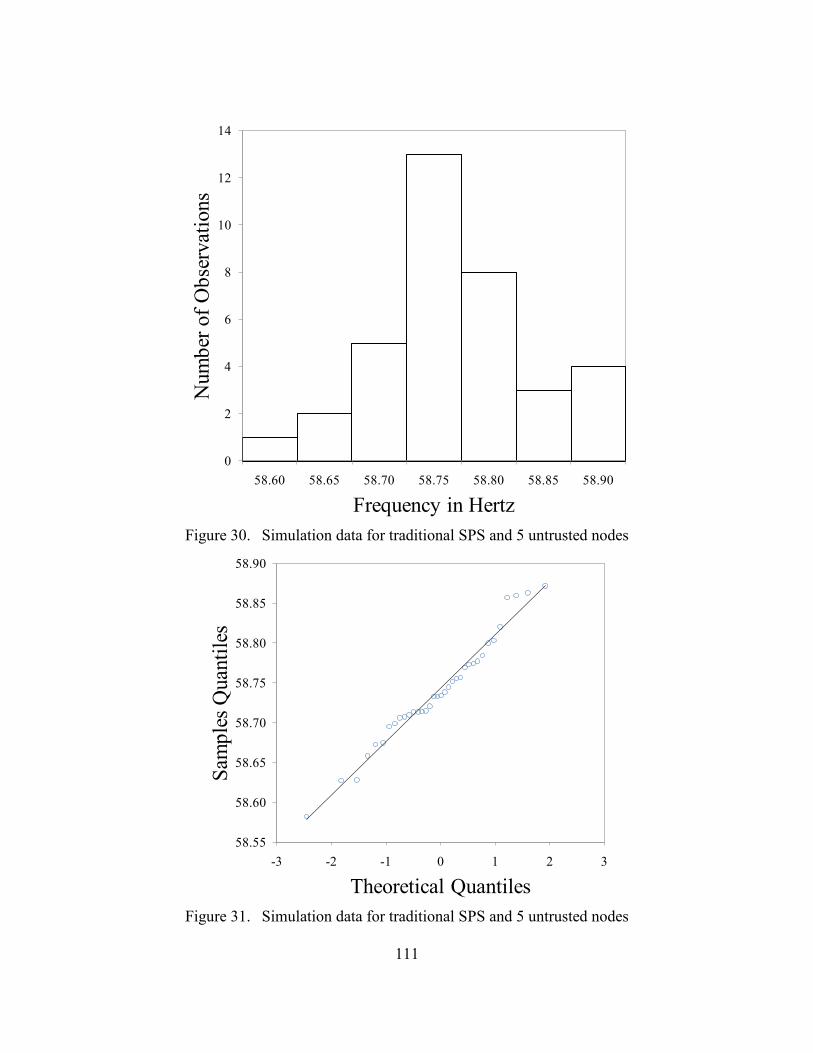
111
Figure 30. Simulation data for traditional SPS and 5 untrusted nodes
Figure 31. Simulation data for traditional SPS and 5 untrusted nodes
0
2
4
6
8
10
12
14
58.60 58.65 58.70 58.75 58.80 58.85 58.90
Num
ber o
f Obs
erva
tions
Frequency in Hertz
58.55
58.60
58.65
58.70
58.75
58.80
58.85
58.90
-3 -2 -1 0 1 2 3
Sam
ples
Qua
ntile
s
Theoretical Quantiles

112
5.6 Simulation Results
The results from the backup protection system scenarios conducted in PSCAD are
fully covered in chapters 3 and 4, as well as in [48] and [59], but are also summarized in
this section. This is followed by a discussion of the results from the special protection
system experiments conducted in PSS/E.
5.6.1 Backup Protection System Scenario Results
The trust management toolkit enhanced backup protection system was able to
detect, initiate corrective action and isolate a faulty power line between nodes S5 and S6
by commanding the software agents located at nodes S3 and S7 to engage their line
breakers. The improved response time of the trust management toolkit enhanced backup
protection system, see Figure 32, is enabled by the improved communications capabilities
of smart grid technologies. The traditional backup protection system without the trust
management toolkit can also correct the problem but must wait a predetermined amount
of time for S5 and S6 to respond to the problem. If S5 and S6 fail to respond, then the
next nodes (S4 and S7) are tasked with engaging their line breakers to correct the
problem. If S7 succeeds in engaging its line breaker but S4 fails to engage its line breaker,
then S3 is tasked with engaging its line breaker—as a backup to S4. In this backup
protection system scenario, it takes approximately 1.5 seconds for the traditional backup
protection system to isolate the faulty line, see Figure 33. These results indicate a 99 %
improvement in backup protection system response time and warranted further study;
namely the larger (145 node) special protection system test case.

113
Figure 32. The trust management toolkit enhanced backup protection system isolates the
faulty line quickly—in ~0.022 seconds
Figure 33. Traditional backup protection system isolates the faulty line in ~1.5 seconds
5.6.2 Special Protection System Scenario Results
The trust management toolkit enhanced special protection system is able to keep
the power grid’s frequency above 58.8 Hz across all three levels of untrusted nodes;
namely, having 5, 10 or 15 untrusted nodes in the power grid. In the scenario’s runs,
untrusted nodes were also untrustworthy, meaning that they do not shed load when asked
to do so. Figure 34 is a representative run of the trust management toolkit enhanced
special protection system with 15 untrusted nodes. Figure 35 is a representative run of the
traditional special protection system without the trust management toolkit and 15
untrusted nodes. The traditional special protection system (without the trust management
toolkit modules) is not able to keep the power grid’s frequency above 58.8 Hz, while the
-4-202468
0 0.2 0.4 0.6 0.8 1 1.2 1.4 1.6 1.8 2
Phas
e A
Curr
ent
(Kilo
-Am
pere
s)
Simulation Time (Seconds)
-4-202468
0 0.2 0.4 0.6 0.8 1 1.2 1.4 1.6 1.8 2
Phas
e A
Curr
ent
(Kilo
-Am
pere
s)
Simulation Time (Seconds)

114
trust management toolkit enhanced special protection system does keep the frequency
above 58.8 Hz. The results from these representative runs are statistically supported by
Figure 36. This figure shows that on average the trust management toolkit enhanced
special protection system was able to maintain the power grid’s frequency above 58.8 Hz
under all three levels of untrusted nodes, while the traditional special protection system
could not maintain the power grid’s frequency above 58.8 Hz under any of the three
levels of untrusted nodes.
Figure 34. Trust management toolkit enhanced special protection system keeps the
system’s frequency above 58.8 Hz
Figure 35. Traditional special protection system is unable to keeps the grid’s frequency
above 58.8 Hz
57.5
58.0
58.5
59.0
59.5
60.0
60.5
0 10 20 30 40 50
Gen
erat
or 1
10 S
peed
(in
Her
tz)
Simulation Time (in Seconds)
Preset Frequency 58.8 Hz
57.5
58.0
58.5
59.0
59.5
60.0
60.5
0 10 20 30 40 50
Gen
erat
or 1
10 S
peed
(in
Her
tz)
Simulation Time (in Seconds)
Preset Frequency 58.8 Hz

115
As expected, the number of untrusted nodes has no effect on the trust
management toolkit enhanced special protection system. The traditional special
protection system is adversely affected by the untrusted nodes. In particular, as the
number of untrusted nodes increase, so does the detrimental effect on the traditional
special protection system. At a 95% confidence interval it is clear that across the three
levels of untrusted nodes the trust management toolkit enhanced special protection
system has a higher minimum frequency compared to the traditional special protection
system without the trust management toolkit. This highlights the need to include the trust
management toolkit in future smart grid protection systems.
Figure 36. Comparison of test cases with 5, 10 and 15 untrusted nodes
58.30
58.40
58.50
58.60
58.70
58.80
58.90
59.00
5 10 15
Freq
uenc
y in
Her
tz
Number of Bad/Untrusted Nodes
Special Protection System (SPS) without Trust Module Special Protection System (SPS) with Trust Module

116
5.7 Summary
The main contribution of this section is a robust and configurable trust
management toolkit protection system augmentation, which can successfully function in
the presence of untrusted (malfunctioning or malicious) smart grid protection system
nodes. This trust management toolkit combines reputation-based trust with network flow
algorithms to identify and mitigate faulty protection and/or communication components
within a smart grid environment. The utility of this trust management toolkit is validated
through experiments comparing the trust management toolkit modified backup and
special protection systems to the original backup and special protection systems and their
associated ANOVA analysis. The simulation results support the use of the trust
management toolkit in future smart grid protection systems.

117
VI. Conclusions and Recommendations
6.1 Overview
This section summarizes my completed research and provides recommendations
for future work. The summaries entail a brief review of the four developmental spirals,
their objectives and their conclusions. These summaries are followed by an explanation
of the significant contribution of this research with respect to the previously stated
hypothesis. This section concludes with recommendations for future research work in this
area of study.
6.2 Developmental Spirals
The focus of this research is the novel use of Network Flow and Reputation-based
Trust techniques within a distributed Trust Management Toolkit (TMT) to 1) assure the
integrity of the available supervisory control and data acquisition (SCADA) sensor data
and 2) improve the decision making process’s response time and accuracy in clearing or
preventing detected faults caused by malfunctions or malicious failures. Network flow
techniques encompass the network flow optimization problem generators and the network
flow algorithm used to solve these generated problems. Reputation-base trust techniques
are a majority rules trust system which uses shared observed information to determine the
state of the system and the trustworthiness of SCADA components. The focus of this
research is accomplished in four incremental steps (as known as spirals), where each
successive step builds on the accomplishments of the previous steps. The individual
spirals, see Table 7, of development are briefly covered next and fully covered in
chapters 2 – 5.

118
Table 7. Projected Spiral Approach
Spiral Name Research Question
Simple Trust Protocol (FS) What factor contributes most to meeting SCADA timing constraints with this protocol?
Centralized SCADA TMT for PSCAD (TAM) How do we implement reputation-based trust and network flow algorithms in a trust assignment module?
Distributed SCADA TMT for PSCAD (DM1) How do we use network flow algorithms in a decision module?
Distributed SCADA TMT for PSS/E (DM2) How does the Trust Management Toolkit scale up to larger test cases?
Note: SCADA means Supervisory Command And Data Acquisition TMT means Trust Management Toolkit FS is Feasibility Study, TAM is Trust Assignment Module, DM1 is Decision Module Version 1 and DM2 is Decision Module Version 2.
The first spiral answered the question, “How can the trustworthiness of SCADA
information source nodes be determined within a timing constraint of 4 milliseconds (ms)
[25]?” This first spiral was a feasibility study, used to determine if further research in this
area is warranted.
The second spiral answered the question, “How can Network Flow techniques,
utilizing Simple Trust results, be used within a centralized Trust Management Toolkit
(TMT) to mitigate detected SCADA errors/faults?” This spiral implemented the Trust
Assignment Module (TAM) used to ascertain individual node trust values based on the
node’s sensor data information provided to a designated centralized controller node.
The third spiral answered the question, “How can Network Flow techniques,
utilizing Simple Trust results, be used within a distributed Trust Management Toolkit
(TMT) to mitigate detected SCADA errors/faults within PSCAD/EMTDC?” This spiral

119
implemented the first Decision Module utilizing network flow techniques—as opposed
to its use in the TAM of spiral 2—to minimize an objective function representative of the
power grid with a given fault condition. The minimization of the objective function
corresponded to the minimization of damage and down time affecting grid customers.
The fourth spiral answered the question, “How can Network Flow techniques,
utilizing Simple Trust results, be used within a distributed Trust Management Toolkit
(TMT) to mitigate detected SCADA errors/faults within Power System Simulation for
Engineering (PSS/E)?” This spiral considers the scalability of our Trust Management
Toolkit with system frequency as a trust system discriminator in the Trust Assignment
Module and a greedy algorithm in the second Decision Module.
6.3 Research contributions
To summarize my research contributions I begin by restating my thesis, as known
as hypothesis:
Hypothesis: How can network flow techniques and reputation-based trust, coupled with
the increased communications capabilities of Smart Grid technology,
assure Supervisory Control And Data Acquisition (SCADA) sensor data
integrity? This assured SCADA sensor data should improve SCADA
protection systems situational awareness and their decision making
capabilities. The expected measurable improvements of this approach
include the protection system’s response time to detected faults and
resilience to malfunctioning and malicious nodes within the power grid.

120
This research’s contribution is a “robust and configurable trust management
toolkit protection system augmentation to smart grid protection systems, which can
successfully function in the presence of untrusted (malfunctioning or malicious)
nodes.” [71] This trust management toolkit combines reputation-based trust with network
flow algorithms to identify and mitigate faulty protection and/or communication
components within a smart grid environment. The experimental results of the trust
management toolkit confirm our previously stated hypothesis.
Additional contributions to the scientific body of knowledge, in the form of
written and presented peer-reviewed conference papers, a poster board presentation and a
submitted Journal article, are listed in Table 8. The publications generated from this
research disseminate information concerning the results of one or more spiral objectives.
Table 8. List of Publications and Associated Research Spirals
Publications Research Spirals Title Locations FS TAM DM1 DM2
Developing a Trust Based Protocol for a Fault Tolerant Distributive Wireless Network (Poster-board) [80]
Cyber-physical Systems Security Conf.
Simple Trust Protocol for Wired and Wireless SCADA networks [30]
ICIW Conf.
SCADA Trust Management System [48]
WORLDCOMP Conf.
Trust Management and Security in the Future Communication-Based “Smart” Electric Power Grid [59]
HICSS44 Conf.
A Trust Management Toolkit for Smart Grid Protection Systems [71]
Journal Submission
Note: FS is Feasibility Study, TAM is Trust Assignment Module, DM1 is Decision Module Version 1 and DM2 is Decision Module Version 2. = accepted and presented publication, = asked to revise and resubmit publication

121
6.4 Recommendations for Future Research
The recommendations within this subsection involve upgrading the software
programs used in the simulation environment, improving the communication speed of the
EPOCHS runtime interface, model checking the Trust Management Toolkit and
improving the configuration management of the overall simulation environment.
Upgrading the software used in the simulation environment should remove
dependencies on out-dated software items, such as Compaq Visual FORTRAN (CVF).
The current version of PSS/E is 30.3.3 which requires Compaq Visual FORTRAN for the
development of FORTRAN modules used to interface PSSE with NS2. Compaq Visual
FORTRAN has been replaced by Intel Visual FORTRAN (IVF). The newer versions of
PSS/E use the new Intel Visual FORTRAN complier. The additional features available in
the new FORTRAN compiler improves its communications capabilities in mixed
programming scenarios, such as the FORTRAN and C++ mixed programming scenario
between PSS/E and NS2. Needless to say, upgrading PSS/E will require some rewriting
and recompiling of the FORTRAN modules used to communicate with NS2.
This same general logic applies to PSCAD version 4.2.1 being upgraded to
version X4. The current version of PSCAD was released in 2005. Improvements
concerning interoperability have occurred over the last five years that should improve
usability and provide a means for PSCAD to import PSS/E data files for future simulation
possibilities.
The last simulation item to upgrade is NS2 from version 2.29 to version 2.34.
NS2 version 2.34 is more extendable from a software engineering point of view, meaning

122
that internal software classes and header files do not have to be modified to extend their
capabilities. Currently in NS2 version 2.29 the internal classes must be modified by the
users to implement new protocols or new routing algorithms. This makes upgrading from
one version of NS2 to another very difficult. NS2 version 2.34 provides software hooks
to dynamically extend the current list of communication protocols, which eliminates the
need to manually modify the internal software classes and header files. The NS2 upgrade
provides an opportunity to rewrite the NS2 “Agent” software to improve its portability
from one version to another, as well as, its usability, maintainability and extensibility.
The NS2 software agents should be modified to better utilize the network information
and interoperability capabilities between C++ and TCL simulation environments. This
improved interoperability will help future students become familiar with the NS2
software agents.
Another recommendation is improving the EPOCHS communication speed
between NS2 and the power simulators by implementing a memory mapped interface.
This issue is considered difficult due to the mixed language programming and the
memory mapped programming difficulties concerning coordinating access between
concurrent processes to shared memory. To help future developers, an operational
memory mapped (Server—Client architecture) C++ sample code is provided in the
Appendix E.
Model checking of the Trust Management Toolkit algorithm is an additional
recommendation for future work. An initial effort is presented in Appendix H using SPIN
(Simple Promela INterpreter). This initial effort confirms that detected power grid faults

123
are mitigated by the decision module. If the detected fault is validated, then the
appropriate SCADA nodes are commanded to open their line relays and isolate the fault.
If the detected fault is not validated, then it is ignored. An invalidated fault could indicate
a SCADA component malfunction or a possible malicious attack—hence, the need to
ignore the invalidated fault and only report it to the SCADA operators. The SCADA
operators would determine if the invalidated fault is due to an equipment malfunction or a
possible malicious attack. This initial effort also verified that no race conditions or
possible deadlocks exist in the Trust Management Toolkit algorithm. A copy of the SPIN
source code (written in ProMeLa) and the results from three verification runs are
provided in Appendix H.
The final recommendation is to use virtual machines for the Linux and Windows
Operating Systems environments with NS2 and the power simulators pre-installed. The
benefits of using virtual machines include portability, ease of use and improved
configuration management. The portability benefit is self explanatory considering the
ease in providing a copy of the virtual machine image to anyone who needs it for
experimentation and simulation. The “ease of use” refers to the elimination of the
difficulties associated with installing NS2 and then modifying the internal classes and
header files, before including the EPOCHS agents files in the modified make file. The
virtual machine image will not require each student to start from scratch, but instead
provide a working environment for them to start with. The improved configuration
management considers that upgrading to a new version of the simulation software items
is only required once for the creation of a new virtual machine image for all to use. The

124
older virtual machine image can be archived for future reference. The initial development
effort should pay off in the long run by decreasing the student initial start-up/ramp-up
time.
6.5 Conclusion
In conclusion of this research effort, the simulation results support the use of this
trust management toolkit in the future smart grid implementation. This future
implementation should be preceded by additional simulations. Additional simulations are
warranted to further solidify the use of the trust management toolkit by demonstrating its
usefulness in additional test case situations.
The results of this research provides a robust and configurable trust management
toolkit protection system augmentation to smart grid protection systems, which can
successfully function in the presence of untrusted (malfunctioning or malicious) nodes.
This trust management toolkit combines reputation-based trust with network flow
algorithms to identify and mitigate faulty protection and/or communication components
within a smart grid environment. The simulation results support the use of the trust
management toolkit in future smart grid implementations.
The positive simulation results consider one small test cases and one large real
world test case. These two test cases were not chosen randomly and are not representative
of all possible power simulation test cases. Hence, additional simulation experiments
with difference test cases are recommended to further solidify the utility of the Trust
Management Toolkit.

125
The developmental research software must be converted to production ready
software, targeted to a specific set of hardware items; such as, Intelligent Electronic
Devices (IED), specific line breaker relays, specific line sensors, specific generators and
specific network communications equipment. Additionally, the production ready version
of this software should include a means of obfuscating the sensor data to assure personal
privacy rights are not violated.

126
Appendix A Spiral Iteration Development Plan
A.1 Spiral 1, Simple Trust Protocol
Objective: To develop a trust protocol capable of determining trust
values within 4 milliseconds (ms) [25] for all the supervisory
control and data acquisition (SCADA) sensor nodes/relays in
a predetermined network neighborhood.
AF/DoD/Science Impacts: successfully meeting this 4 ms timing constraint enables us to
proceed forward to spiral two. This is the first step in
determining the feasibility of this trust algorithm within a
SCADA network.
Entrance Criteria: All of the following resources must be available and the
following preconditions satisfied before starting this spiral.
Resources: Unlimited access to a computer system with
1) a Linux or Linux like Operating System and
2) sufficient computing power to run Network Simulator 2
(NS2) [32].
Preconditions: Permission to load the following software on the provided
computer system:
1) Linux or Linux like Operating System (e.g., Cygwin [81])
2) Network Simulator 2 (NS2 [32])
3) Network Animator (NAM [47])
4) A OTCL compiler
5) A C/C++ compiler (e.g., gcc/g++)

127
6) A C/C++ debugger (e.g., gdb)
7) A text editor (e.g., VI, VIM, EMACS, Notepad++ …)
8) A scripting language (e.g., PERL, AWK, SED …)
9) A statistical package (e.g., R, Minitab, MS Excel)
10) document preparation software (e.g., MS word, Latex …)
Activities/Contributions: The 2k
Figure 2
factorial activities conducted in this spiral are based
on Dr. Raj Jain’s book “The Art of Computer Systems
Performance Analysis,” where k=3 and represents three
factors being modified, see . The three factors being
modified between a high and low value are bandwidth,
medium and number of malicious nodes resulting in 8
simulations. These simulations enable us to attribute a
percentage of effect to each factor, e.g., changing bandwidth
has a 99% effect on spiral 1 results, while changing the
number of byzantine nodes has 0% effect on spiral 1 results.
Measure of Progress: The measure of progress / readiness to proceed to the next
spiral is determined by the results indicating the ability to
meet the 4 ms timing constraint.
Exit Criteria: At the conclusion of this spiral, the Simple Trust algorithm
can be shown to meet or not meet the 4 ms timing constraint
[25] within a abstract representation of a SCADA WAN
environment.

128
Deliverables: This spiral’s deliverables are the simple trust algorithm, a
report assessing the simple trust protocol and a publication
demonstrating the simple trust protocol.

129
A.2 Spiral 2, Centralized SCADA Trust Management System for PSCAD
Objective: The objectives of this spiral are:
1. Learn PSCAD [31] software
2. Learn EPOCHS [24] software
3. Add PSCAD supervisory control and data acquisition
(SCADA) Trust Management System (TMS) agents to
EPOCHS [24] software
4. Develop a centralized PSCAD SCADA TMS
5. Develop a PSCAD rule set for the SCADA TMS
AF/DoD/Science Impacts: successfully completing this second spiral enables us to
proceed forward to spiral three. This second step provides a
centralized SCADA TMS capable of detecting and mitigation
malicious and byzantine node’s sensor data. SCADA TMS
helps protect the nation’s power grid from malicious attacks
and insures electric power is available for AF and DoD uses.
Entrance Criteria: Successful completion of spiral 1 and the all of the following
resources must be available and the following preconditions
satisfied before starting this spiral.
Resources: Unlimited access to a computer system with
1) a Windows Operating System (e.g., Windows XP) and
2) a Linux like Operating System (e.g., Cygwin) and
3) sufficient computing power to run Network Simulator 2

130
(NS2) [32], and PSCAD [31].
Access to PSCAD test cases is also required for this spiral.
Preconditions: Permission to load the following software on the provided
computer system:
1) a Windows Operating System (e.g., Windows XP)
2) a Linux like Operating System (e.g., Cygwin [81])
3) Network Simulator 2 (NS2 [32])
4) Network Animator (NAM [47])
5) A OTCL compiler
6) A C/C++ compiler (e.g., gcc/g++)
7) A C/C++ debugger (e.g., gdb)
8) A text editor (e.g., VI, VIM, EMACS, Notepad++ …)
9) A scripting language (e.g., PERL, AWK, SED …)
10) A statistical package (e.g., R, Minitab, MS Excel)
11) document preparation software (e.g., MS word, Latex …)
12) PSCAD [31]
13) A Fortran compiler (e.g., F77, G77, Intel Fortran …)
Activities/Contributions: 1. Examine the PSCAD and EPOCHS source code to gain an
understanding of the information available.
2. Modify the PSCAD and EPOCHS source code as needed
to implement simple trust and SCADA TMS.
3. Implement a centralized version of SCADA TMS

131
4. Demonstrate the SCADA TMS with the four PSCAD test
cases.
Measure of Progress: The measure of progress / readiness to proceed to the next
spiral is determined by the successful development of the
centralized version of SCADA TMS for PSCAD.
Exit Criteria: The successful development of a centralized version of
SCADA TMS demonstrated within PSCAD and NS2
utilizing EPOCHS.
Deliverables: This spiral’s deliverables are a centralized SCADA TMS
implementation and a publication demonstrating the
capabilities of SCADA TMS.

132
A.3 Spiral 3, Distributed SCADA Trust Management System for PSCAD
Objective: The objective of this spiral is to develop a distributed
supervisory control and data acquisition (SCADA) Trust
Management System (TMS) for Power Systems Computer
Aided Design (PSCAD)/ElectroMagnetic Transients
including Direct Current (EMTDC).
AF/DoD/Science Impacts: successfully completing this third spiral enables us to
proceed forward to spiral four. This third step provides a
distributed SCADA TMS capable of detecting and mitigation
malicious and byzantine node’s sensor data. SCADA TMS
helps protect the nation’s power grid from malicious attacks
and insures electric power is available for AF and DoD uses.
Entrance Criteria: Successful completion of spiral 2 and the all of the following
resources must be available and the following preconditions
satisfied before starting this spiral.
Resources: Same as Spiral 2 Resources.
Preconditions: Same as Spiral 2 Preconditions.
Activities/Contributions: 1. Modify the PSCAD and EPOCHS source code as needed
to implement a distributed version of SCADA TMS.
2. Demonstrate SCADA TMS with the four PSCAD test
cases.

133
Measure of Progress: The measure of progress / readiness to proceed to the next
spiral is determined by the successful development of the
distributed version of SCADA TMS for PSCAD.
Exit Criteria: The successful development of a distributed version of
SCADA TMS demonstrated within PSCAD and NS2
utilizing EPOCHS.
Deliverables: This spiral’s deliverables are a distributed SCADA TMS
implementation and part of a journal publication
demonstrating the capabilities of SCADA TMS.

134
A.4 Spiral 4, Distributed SCADA Trust Management System for PSS/E
Objective: The objectives of this spiral are:
1. Learn PSSE [82] software
2. Add PSSE [82] SCADA supervisory control and data
acquisition (SCADA) Trust Management System (TMS)
agents to EPOCHS [24] software
3. Develop a distributed PSSE [82] SCADA TMS
4. Develop a PSSE [82] rule set for the SCADA TMS
AF/DoD/Science Impacts: successfully completing of this spiral provides a distributed
SCADA TMS capable of detecting and mitigation malicious
and byzantine node’s sensor data. SCADA TMS helps
protect the nation’s power grid from malicious attacks and
insures electric power is available for AF and DoD uses.
Entrance Criteria: Successful completion of spiral 3 and the all of the following
resources must be available and the following preconditions
satisfied before starting this spiral.
Resources: Unlimited access to a computer system with
1) a Windows Operating System (e.g., Windows XP) and
2) a Linux like Operating System (e.g., Cygwin) and
3) sufficient computing power to run Network Simulator 2
(NS2) [32], and PSSE [82].
Access to PSSE test cases is also required for this spiral.

135
Preconditions: Permission to load the following software on the provided
computer system:
1) a Windows Operating System (e.g., Windows XP)
2) a Linux like Operating System (e.g., Cygwin [81])
3) Network Simulator 2 (NS2 [32])
4) Network Animator (NAM [47])
5) A OTCL compiler
6) A C/C++ compiler (e.g., gcc/g++)
7) A C/C++ debugger (e.g., gdb)
8) A text editor (e.g., VI, VIM, EMACS, Notepad++ …)
9) A scripting language (e.g., PERL, AWK, SED …)
10) A statistical package (e.g., R, Minitab, MS Excel)
11) document preparation software (e.g., MS word, Latex …)
12) PSSE [82]
Activities/Contributions: 1. Learn PSS/E capabilities concerning input files and results
2. Modify the TCL script generator for given PSS/E circuits
3. Examine the PSSE and EPOCHS source code to gain an
understanding of the information available.
4. Determine how to partition the power grid topology into
overlapping network neighborhoods.
5. Create new rule set based on PSS/E available information
6. Modify the graph building algorithm to handle cycles in
the power grid topology.

136
7. Create new EPOCHS agents for PSS/E, employing
distributed SCADA TMS.
Measure of Progress: The measure of progress is determined by the successful
development of the distributed version of SCADA TMS for
PSSE.
Exit Criteria: The successful development of a distributed version of
SCADA TMS demonstrated within PSSE and NS2 utilizing
EPOCHS.
Deliverables: This spiral’s deliverables are a distributed SCADA TMS
implementation and part of a journal publication
demonstrating the capabilities of SCADA TMS

137
Appendix B HIPR Flow Algorithm Modifications
The capability to locate and enumerate all minimum cutsets was added to the
High-Level Push-Relabel (HIPR) flow algorithm [55]. This added capability is described
in [56] and illustrated here with a graph from [27] page 398. In addition, further
miscellaneous changes were made to improve usability, such as, adding an "end"
statement to signify the end of the input stream.
In chapter 3, it was stated that SCADA TMS uses trust information to make better
decision concerning detected fault resolutions. The initially developed trust values, using
Simple Trust protocol [30], were further refined using network flow techniques (e.g.,
image segmentation or image labeling) to detect false positives and false negatives trust
assignments. A false positive is defined to be a non-malicious trust agent assigned a low
trust value. A false negative is defined as a malicious trust agent assigned a high trust
value.
Detecting false positives and false negatives trust assignments is accomplished by
determining the minimum cutset of the resulting graph, which becomes problematic when
more than one minimum cutset exist. This problem is resolved by identifying all the
minimum cutsets in the graph and selecting the one which results in a minimal change in
assigned trust values. It is anticipated that the trust values assigned to SCADA sensor
node/relays change slowly over time. Hence, the minimum cutset with the minimal
difference in assigned trust values is probably correct.
The capability to identify all minimum cutsets in a given graph from [56] was
added to HIPR [55]. Originally, HIPR identified only one minimum cutset—the cutset
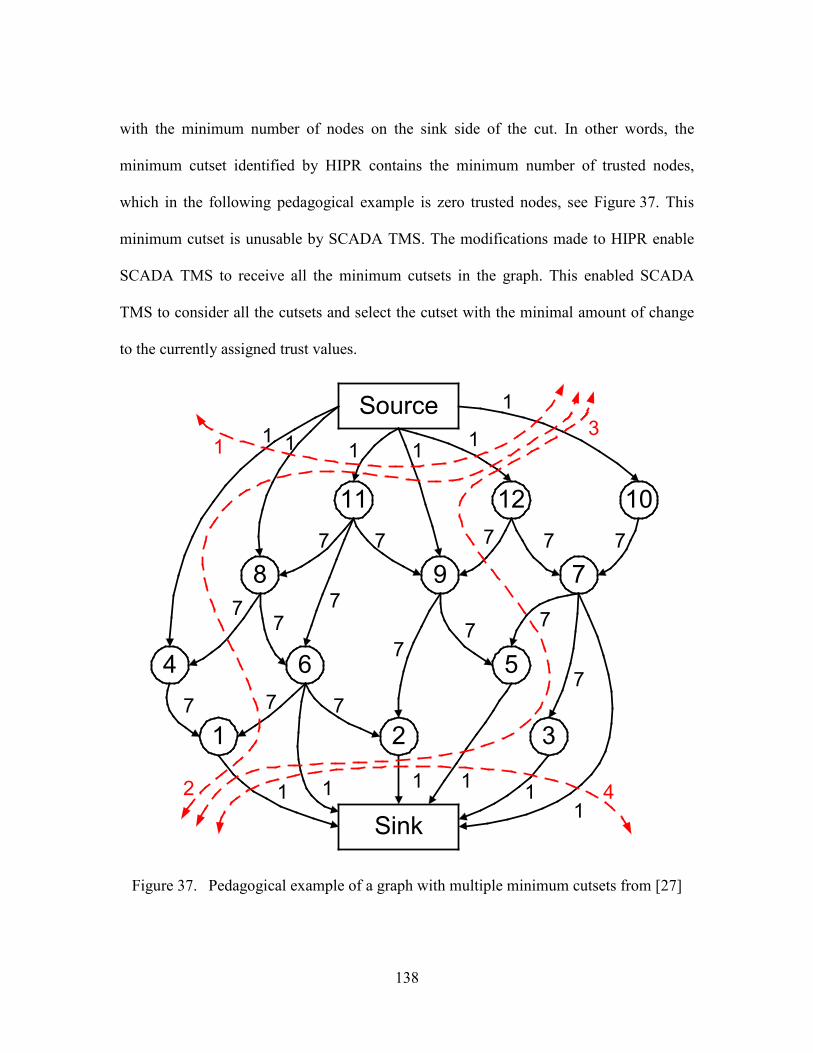
138
with the minimum number of nodes on the sink side of the cut. In other words, the
minimum cutset identified by HIPR contains the minimum number of trusted nodes,
which in the following pedagogical example is zero trusted nodes, see Figure 37. This
minimum cutset is unusable by SCADA TMS. The modifications made to HIPR enable
SCADA TMS to receive all the minimum cutsets in the graph. This enabled SCADA
TMS to consider all the cutsets and select the cutset with the minimal amount of change
to the currently assigned trust values.
Figure 37. Pedagogical example of a graph with multiple minimum cutsets from [27]
Source
11
Sink
12 10
8
4
1
9 7
6 5
2 3
1 1 1 1 1
1
1 11 1 11
7
77
7 7
7
77
7 7 7 7 7
7
7
4
3
2
1

139
The pedagogical example in Figure 37 is a modified version of the graph in
Kleinberg and Tardos algorithms book [27] page 398. The nodes in the graph have
assigned identification numbers and the edges have assigned cost values. The four
minimum cutsets are identified by the red dashed lines in Figure 37. The corresponding
HIPR program input and output files are shown in Figure 38 and Figure 39, respectively.
The “nodes on the source side” in Figure 39 is the resulting output of the additional
algorithm from [56]. The nodes on the source side of the minimum cutset represent the
untrusted nodes in the graph. Minimum cutset 4 corresponds to HIPR’s unmodified
results, which indicates that all the nodes (1-12) are untrusted. The added capability of
the modified HIPR program provides the means to selecte the correct minimum cutset.
Figure 38. HIPR program input file for the graph in Figure 37.
p max 14 27 n 13 s n 14 t a 1 14 1 a 2 14 1 a 3 14 1 a 4 1 7 a 5 14 1 a 6 1 7 a 6 14 1 a 6 2 7 a 7 14 1 a 7 3 7 a 7 5 7 a 8 4 7 a 8 6 7 a 9 2 7 a 9 5 7 a 10 7 7 a 11 6 7 a 11 8 7 a 11 9 7 a 12 7 7 a 12 9 7 a 13 10 1 a 13 11 1 a 13 12 1 a 13 4 1 a 13 8 1 a 13 9 1

140
Figure 39. HIPR program output file for the graph in Figure 37.
c c hi_pr version 3.6 c Copyright C by IG Systems, [email protected] c c nodes: 14 c arcs: 27 c c flow: 6.0 c time: 0.00 c cut tm: 0.00 c c Solution checks (feasible and optimal) c c pushes: 33 c relabels: 15 c updates: 2 c gaps: 0 c gap nodes: 0 c c flow values f 1 14 1 f 2 14 1 f 3 14 1 f 4 1 1 f 5 14 1 f 6 2 0 f 6 14 1 f 6 1 0 f 7 14 1 f 7 5 0 f 7 3 1 f 8 6 1 f 8 4 0 f 9 2 1 f 9 5 1 f 10 7 1 f 11 8 0 f 11 9 1 f 11 6 0 f 12 7 1 f 12 9 0 f 13 4 1 f 13 10 1 f 13 8 1 f 13 11 1 f 13 9 1 f 13 12 1 c c nodes on the sink side c 14 c c nodes on the source side c 1 ->{ 13 } c 2 ->{ 4 1 13 } c 3 ->{ 11 9 8 6 5 2 4 1 13 } c 4 ->{ 12 10 7 3 11 9 8 6 5 2 4 1 13 } c

141
Minimum Cutset 1
Minimum Cutset 2
Minimum Cutset 3
Minimum Cutset 4
Figure 40. The four minimum cutsets corresponding to the graph in Figure 37
The four minimum cutsets shown in Figure 40 graphically represent the untrusted
nodes (filled in circles) and the trusted nodes (unfilled circles) corresponding to HIPR’s
results in Figure 39. The assigned trust values from the previous iteration of SCADA
TMS are used to select the appropriate minimum cutset to be used in the current iteration.
For example, if all the nodes were trusted in the previous SCADA TMS iteration, then
minimum cutset 1 would be used in the current SCADA TMS iteration.
Source
11
Sink
12 11
8
4
1
9 7
6 5
2 3
1
1
1
1
11
111 1
11
1
1
1
11
1 1
1
Source
11
Sink
12 11
8
4
1
9 7
6 5
2 3
1
1
1
1
11
111 1
11
1
1
1
11
1 1
1
Source
11
Sink
12 11
8
4
1
9 7
6 5
2 3
1
1
1
1
11
111 1
11
1
1
1
11
1 1
1
Source
11
Sink
12 11
8
4
1
9 7
6 5
2 3
1
1
1
1
11
111 1
11
1
1
1
11
1 1
1

142
Appendix C Network Generation Algorithms
The network graph generation algorithms discussed in chapter 4 are capable of
handling acyclic SCADA connectivity networks, i.e. power grid networks without loops.
For example, the network in Figure 41 represents an acyclic SCADA connectivity
network. If faults are detected between sensor node/relays <S4, S5>, <S11, S12>, or
<S8, S9>, then the corresponding graphs solved by Dijkstra’s shortest path algorithm are
shown in Figure 43, Figure 44, and Figure 45, respectively. A cyclic SCADA
connectivity network, see Figure 42, is not currently handled by these network generation
algorithms.
Figure 41. Representative acyclic SCADA connectivity network
Figure 42. Representative cyclic SCADA connectivity network
HS1
HS2
HS3
HS7
HS8
High Voltage LineH = Trusted Node
L = Untrusted Node
Legend: = Sensor nodes/relays, = Power Generator, = Power Bus
LS4
LS5
LS6
HS9
HS10
HS11
HS12
HS13
HS14
HS20
HS16
HS17
LS15
HS18
HS19
HS1
HS2
HS3
HS7
HS8
High Voltage LineH = Trusted Node
L = Untrusted Node
Legend: = Sensor nodes/relays, = Power Generator, = Power Bus
LS4
LS5
LS6
HS9
HS10
HS11
HS12
HS13
HS14
HS20
HS16
HS17
LS15
HS18
HS19
HS21
HS22

143
Figure 43. Resulting graph for a detected fault between nodes <S4, S5> in Figure 41.
Figure 44. Resulting graph for a detected fault between nodes <S11, S12> in Figure 41.
HS1
HS2
HS3
HS7
HS8
H = Trusted Node
L = Untrusted Node
LEGEND
= Sensor nodes/relays
= Artificial nodes used to signifythe source node, sink nodeand various junction nodes
LS4
LS5
LS6
HS9
HS10
HS11
HS12
HS13
HS14
HS20
HS16
HS17
LS15
HS18
HS19
LS R
TJ1 J2 J3
J4 J5 J6
Directional Edges
HS1
HS2
HS3
HS7
HS8
H = Trusted Node
L = Untrusted Node
LEGEND
= Sensor nodes/relays
= Artificial nodes used to signifythe source node, sink nodeand various junction nodes
LS4
LS5
LS6
HS9
HS10
HS11
HS12
HS13
HS14
HS20
HS16
HS17
LS15
HS18
HS19
LS
R
T
J1 J2 J3
J4 J5 J6Directional Edges

144
Figure 45. Resulting graph for a detected fault between nodes <S8, S9> in Figure 41.
HS8
HS7
HS6
HS2
HS3
H = Trusted Node
L = Untrusted Node
LEGEND
= Sensor nodes/relays
= Artificial nodes used to signifythe source node, sink node
and various junction nodes
LS10
LS9
LS1
HS4
HS5
HS11
HS12
HS13
HS14
HS20
HS16
HS17
LS15
HS18
HS19
LS
R T
J1 J2
J3
J4 J5 J6
Directional Edges

145
Appendix D Compensating for Network Delay and Coordination Errors
The objective of spiral 3 is “to develop a distributed SCADA TMS for PSCAD /
EMTDC”. Network delay and message coordination errors between network nodes were
encountered during this spiral of development. Explaining this problem and the plan for
solving this problem is where this section begins.
D.1 The Network Delay and Coordination Problem
The change from a centralized SCADA TMS for PSCAD increased the amount of
network packet communication traffic from 16 packets per round to 50 packets per round,
where a round represents a single simulation time-step of 2 milliseconds (ms). The
16 packets per round represent a message sent by each sensor node/relay to the
centralized SCADA TMS process control system node and a response message sent from
the SCADA TMS process control system node back to each sensor node/relay, see
Figure 46. The 16 packets were able to traverse the communications network within the
2 ms simulation time-step. The distributed SCADA TMS implementation for PSCAD
increased the network communications traffic between the sensor nodes/relays, gateway
nodes and process control node, see Figure 47. This abstract hierarchical configuration is
used to develop sensor node/relay trust values. Recall that the sensor node/relays run the
SCADA TMS algorithm on a subset of the entire network based on a maximum hop
distance, hmax
Figure 47
, discussed in the previous chapter 4, which utilizes the trust values
developed by this abstract hierarchical configuration. In , each gateway node
communicates with 4 sensor nodes/relays, i.e., each gateway node sends and receives a
total of 8 packets of data per round. Hence, the three gateway nodes account for
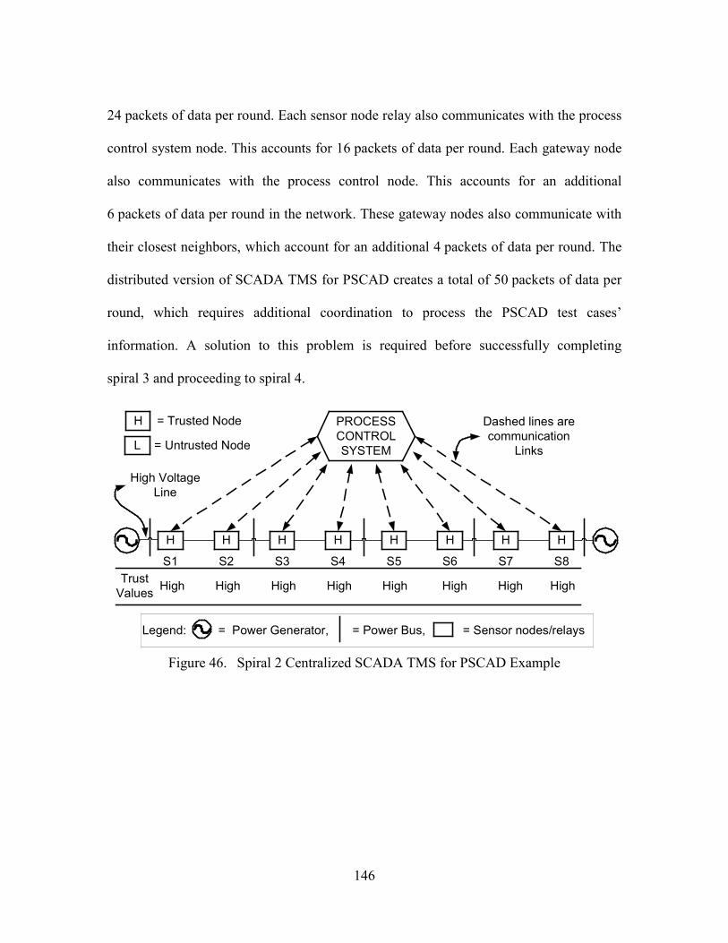
146
24 packets of data per round. Each sensor node relay also communicates with the process
control system node. This accounts for 16 packets of data per round. Each gateway node
also communicates with the process control node. This accounts for an additional
6 packets of data per round in the network. These gateway nodes also communicate with
their closest neighbors, which account for an additional 4 packets of data per round. The
distributed version of SCADA TMS for PSCAD creates a total of 50 packets of data per
round, which requires additional coordination to process the PSCAD test cases’
information. A solution to this problem is required before successfully completing
spiral 3 and proceeding to spiral 4.
Figure 46. Spiral 2 Centralized SCADA TMS for PSCAD Example
PROCESSCONTROLSYSTEM
H
S1
H
S2
H
S3
H
S4
H
S5
H
S6
H
S7
H
S8
High High High High High High High HighTrustValues
Dashed lines arecommunication
Links
High VoltageLine
H = Trusted Node
L = Untrusted Node
Legend: = Power Generator, = Power Bus, = Sensor nodes/relays

147
Figure 47. Spiral 3 Distributed SCADA TMS for PSCAD Example
The possible solutions to this network delay and coordination problem include;
1) adding a Global Positioning System (GPS) timestamp to each packet message,
2) using a pipelining approach, 3) using a reduce and forward astrolabe approach or 4)
adding a buffer to the gateway nodes and the process control system node. Each approach
has an associated cost in terms of time, money, complexity and difficulty. In this
theoretical / simulation environment the pipelining solution is selected because of the
author’s familiarity with this technique and its minimal complexity and minimal
difficulty. If this solution does not correct the problem, then one of the other two possible
solutions will be tried.
D.2 Pipelining Solution
The pipelining solution is intended to correct the network propagation delay
problem experienced in the distributed SCADA TMS for PSCAD network simulations.
PROCESSCONTROLSYSTEM
G1 G2 G3
H
S1
H
S2
H
S3
H
S4
H
S5
H
S6
H
S7
H
S8
High High High High High High High HighTrustValues
Dashed lines arecommunication
Links
High VoltageLine
H = Trusted Node
L = Untrusted Node
Legend: = Sensor nodes/relays, = Gateway Node,
= Power Generator, = Power Bus
G#

148
This problem is identified by the lack of coordination in the received network packets.
For example, the 8 sensor nodes/relays send their data packets to the gateway nodes and
the process control system node in the same round (say round 2), but it takes different
amounts of time to propagate through the network. Hence, the received messages arriving
during different rounds, e.g., round 2 message from sensor node/relay 3 may arrive at the
process control system node in round 2, while round 2 messages from sensor nodes/relays
5 and 6 arrive in round 5. The pipelining solution synchronizes the transfer of
information from one level to the next, e.g., from the sensor nodes/relays to the gateway
nodes. This reduces the amount of network packet communication traffic from 46 packets
per round to 30 packets per round. The pipelining solution limits the distant traveled per
round to one hop. This should correct the coordination issues created by the varying
network propagation delays.
Figure 48 through Figure 51, illustrate the pipelining process. Figure 48 shows
round 1 information sent from the sensor nodes/relays to the gateway nodes. Figure 49
shows the round 1 information sent from the gateway nodes to the process control system
node and round 2 information sent from the sensor nodes/relays to the gateway nodes.
Figure 50 shows round 1 response message sent from the process control system node to
the gateway nodes, round 2 information sent to the process control node from the
gateway nodes and round 3 information sent from the sensor nodes/relays to the gateway
nodes. Figure 51 show the full amount of network traffic in one round; namely, round 1
response message from the gateway nodes sent to the sensor nodes/relays, round 2
response message sent from the process control system node to the gateway nodes,
round 3 information sent from the gateway nodes to the process control system nodes and
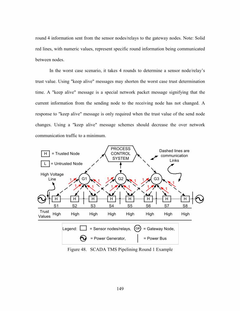
149
round 4 information sent from the sensor nodes/relays to the gateway nodes. Note: Solid
red lines, with numeric values, represent specific round information being communicated
between nodes.
In the worst case scenario, it takes 4 rounds to determine a sensor node/relay’s
trust value. Using "keep alive" messages may shorten the worst case trust determination
time. A "keep alive" message is a special network packet message signifying that the
current information from the sending node to the receiving node has not changed. A
response to "keep alive" message is only required when the trust value of the send node
changes. Using a "keep alive" message schemes should decrease the over network
communication traffic to a minimum.
Figure 48. SCADA TMS Pipelining Round 1 Example
PROCESSCONTROLSYSTEM
G1 G2 G3
H
S1
H
S2
H
S3
H
S4
H
S5
H
S6
H
S7
H
S8
High High High High High High High HighTrustValues
Dashed lines arecommunication
Links
High VoltageLine
H = Trusted Node
L = Untrusted Node
Legend: = Sensor nodes/relays, = Gateway Node,
= Power Generator, = Power Bus
G#
11
11
11 1
1
1
1
11
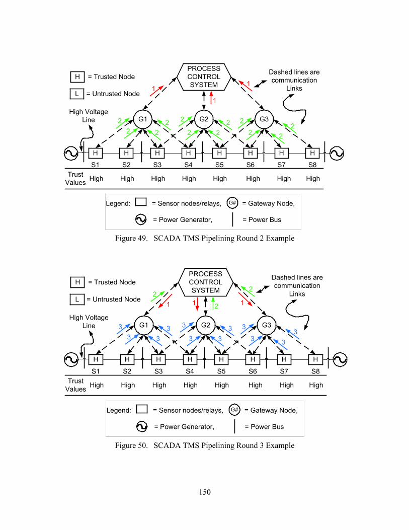
150
Figure 49. SCADA TMS Pipelining Round 2 Example
Figure 50. SCADA TMS Pipelining Round 3 Example
PROCESSCONTROLSYSTEM
G1 G2 G3
H
S1
H
S2
H
S3
H
S4
H
S5
H
S6
H
S7
H
S8
High High High High High High High HighTrustValues
Dashed lines arecommunication
Links
High VoltageLine
H = Trusted Node
L = Untrusted Node
Legend: = Sensor nodes/relays, = Gateway Node,
= Power Generator, = Power Bus
G#
22
22
22 2
2
2
2
22
11
1
PROCESSCONTROLSYSTEM
G1 G2 G3
H
S1
H
S2
H
S3
H
S4
H
S5
H
S6
H
S7
H
S8
High High High High High High High HighTrustValues
Dashed lines arecommunication
Links
High VoltageLine
H = Trusted Node
L = Untrusted Node
Legend: = Sensor nodes/relays, = Gateway Node,
= Power Generator, = Power Bus
G#
33
33
33 3
3
3
3
33
22
21 11

151
Figure 51. SCADA TMS Pipelining Round 4 Example
PROCESSCONTROLSYSTEM
G1 G2 G3
H
S1
H
S2
H
S3
H
S4
H
S5
H
S6
H
S7
H
S8
High High High High High High High HighTrustValues
Dashed lines arecommunication
Links
High VoltageLine
H = Trusted Node
L = Untrusted Node
Legend: = Sensor nodes/relays, = Gateway Node,
= Power Generator, = Power Bus
G#
44
44
44 4
4
4
4
44
33
32 22
1111 111 11111
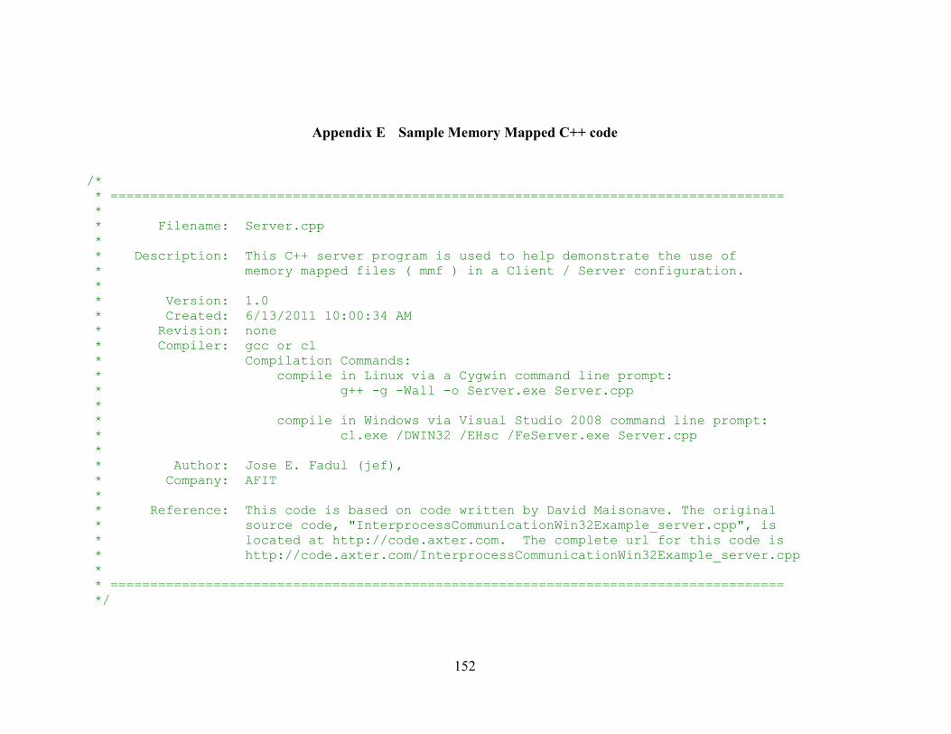
152
Appendix E Sample Memory Mapped C++ code
/* * ===================================================================================== * * Filename: Server.cpp * * Description: This C++ server program is used to help demonstrate the use of * memory mapped files ( mmf ) in a Client / Server configuration. * * Version: 1.0 * Created: 6/13/2011 10:00:34 AM * Revision: none * Compiler: gcc or cl * Compilation Commands: * compile in Linux via a Cygwin command line prompt: * g++ -g -Wall -o Server.exe Server.cpp * * compile in Windows via Visual Studio 2008 command line prompt: * cl.exe /DWIN32 /EHsc /FeServer.exe Server.cpp * * Author: Jose E. Fadul (jef), * Company: AFIT * * Reference: This code is based on code written by David Maisonave. The original * source code, "InterprocessCommunicationWin32Example_server.cpp", is * located at http://code.axter.com. The complete url for this code is * http://code.axter.com/InterprocessCommunicationWin32Example_server.cpp * * ===================================================================================== */

153
#pragma warning(disable: 4786) #include <stdlib.h> #include <cstdlib> #include <iostream> #include <windows.h> #include <string> /* * ===================================================================================== * Class: DataExchange * Description: Abstract Class used to define the main two functions required in * Exchanging Data, namely, SendData( ... ) and GetData( ... ). * ===================================================================================== */ class DataExchange { public: virtual ~DataExchange(){} virtual bool SendData(const char* Data, int Qty) = 0; virtual bool GetData(char* Data, int &Qty)=0; inline int GetErrorID(){return ErrorID;} protected: int ErrorID; }; /* * ===================================================================================== * Class: MapMemExchange * Description: An implementation Class of the DataExchange abstract class. * ===================================================================================== */ class MapMemExchange : public DataExchange {

154
public: // A few constant enums used to help document the code, i.e., "OPEN_MP" is more // descriptive than "0" and "CREATE_MP" is more descriptive than "1". enum OPEN_MODE{OPEN_MP, CREATE_MP}; enum EXCH_STAT{EMPTY_DATA, FETCH_DATA}; enum {DATA_INDEX = 1 + sizeof(int)}; // Notice the enum trick used here // to define a constant. This constant // specifies the data's starting memory // location. /* *-------------------------------------------------------------------------------------- * Class: MapMemExchange * Method: MapMemExchange :: MapMemExchange * Description: This method instantiates a MapMemExchange object given a name, size and * mode. * Inputs: const std::string &Name is the name of the memory mapped file. * int Size is the amount of memory to allocate to this * memory mapped filed. * OPEN_MODE mode is one of two desired memory mapped actions, * i.e., OPEN_MP to open a previously allocated * memory mapped located or CREATE_MP to allocate * memory for a memory mapped filed. *-------------------------------------------------------------------------------------- */ MapMemExchange(const std::string &Name, int Size, OPEN_MODE mode) :m_Name(Name), m_MapPtr(NULL), m_MapHandle(NULL), m_Size(Size), m_mode(mode) { m_MapHandle = (m_mode == CREATE_MP)? CreateFileMapping(INVALID_HANDLE_VALUE, NULL, PAGE_READWRITE, 0, m_Size + DATA_INDEX, m_Name.c_str()): OpenFileMapping(FILE_MAP_ALL_ACCESS, TRUE, m_Name.c_str());

155
if (m_MapHandle != INVALID_HANDLE_VALUE) { m_MapPtr = (char*)MapViewOfFile(m_MapHandle, FILE_MAP_ALL_ACCESS, 0, 0, m_Size + DATA_INDEX); if (m_mode == CREATE_MP && m_MapPtr) { m_MapPtr[0] = EMPTY_DATA; memset(m_MapPtr+1, 0, sizeof(int)); } } } /* *-------------------------------------------------------------------------------------- * Class: MapMemExchange * Method: MapMemExchange :: SendData * Description: This is an implementation of the SendData virtual method defined in * the DataExchange abstract class. * Inputs: const char* Data is the character array written to the memory mapped * file location. * int Qty is the size of the given Data array. *-------------------------------------------------------------------------------------- */ bool SendData(const char* Data, int Qty) { if (!m_MapPtr) return false; // Spin lock used to wait until the memory mapped file location is free while(m_MapPtr[0] != EMPTY_DATA) { Sleep(0); } // copy the Data into the memory mapped filed location
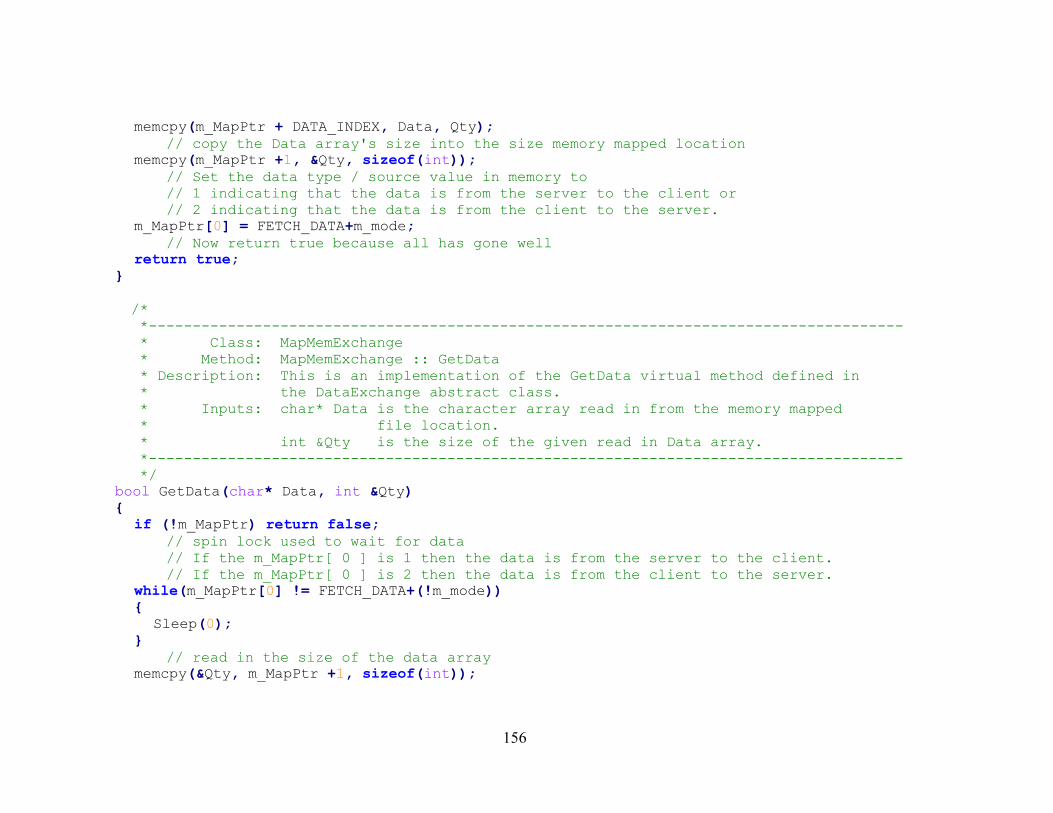
156
memcpy(m_MapPtr + DATA_INDEX, Data, Qty); // copy the Data array's size into the size memory mapped location memcpy(m_MapPtr +1, &Qty, sizeof(int)); // Set the data type / source value in memory to // 1 indicating that the data is from the server to the client or // 2 indicating that the data is from the client to the server. m_MapPtr[0] = FETCH_DATA+m_mode; // Now return true because all has gone well return true; } /* *-------------------------------------------------------------------------------------- * Class: MapMemExchange * Method: MapMemExchange :: GetData * Description: This is an implementation of the GetData virtual method defined in * the DataExchange abstract class. * Inputs: char* Data is the character array read in from the memory mapped * file location. * int &Qty is the size of the given read in Data array. *-------------------------------------------------------------------------------------- */ bool GetData(char* Data, int &Qty) { if (!m_MapPtr) return false; // spin lock used to wait for data // If the m_MapPtr[ 0 ] is 1 then the data is from the server to the client. // If the m_MapPtr[ 0 ] is 2 then the data is from the client to the server. while(m_MapPtr[0] != FETCH_DATA+(!m_mode)) { Sleep(0); } // read in the size of the data array memcpy(&Qty, m_MapPtr +1, sizeof(int));

157
// read in the data array memcpy(Data, m_MapPtr + DATA_INDEX, Qty); // Set the data type / source value in memory to // 0 indicating that the memory location is free. m_MapPtr[0] = EMPTY_DATA; // return true indicating that the memory mapped data was read in successfully. return true; } /* *-------------------------------------------------------------------------------------- * Class: MapMemExchange * Method: MapMemExchange :: ~MapMemExchange * Description: This method is used to destroy the MapMemExchange object. * Inputs: None *-------------------------------------------------------------------------------------- */ ~MapMemExchange() { if (m_MapPtr) UnmapViewOfFile(m_MapPtr);; if (m_MapHandle) CloseHandle(m_MapHandle);; } private: const std::string m_Name; // name of the memory mapped filed location const int m_Size; // size of the memory mapped filed location char *m_MapPtr; // this is a pointer to the beginning of the memory mapped // file location HANDLE m_MapHandle; // This is a handle to the memory mapped file location const OPEN_MODE m_mode; // This is the mode used to access the memory mapped file // file location. };

158
/* * === FUNCTION ====================================================================== * Name: main * Description: This is the main entry point for the server program. * Inputs: int argc is the number of command line arguments * char *argv[] is the array of command line arguments * * NOTE: The command line argument expected is an optional non-negative integer, * which determines the number of rounds between the server and the * client, where a round consist of two sent and two received messages, * i.e., 4 exchanges of data. * If no argument is given, then the default value of 6 is used. * ===================================================================================== */ int main ( int argc, char *argv[] ) { // The name of the memory mapped file location const char NameOfMyMapView[] = "TestingAppCommunication"; // The amount of memory requested for the memory mapped file location const int SizeOfBuffer = 5000; // local variables used to hold the received message and its size char Buff[SizeOfBuffer]; int FetchQty = sizeof(Buff); int round = 0; // used to track the number of rounds. // messages sent to client from server const char* DataToSend1 = "George"; const char* DataToSend2 = "Request"; const char* DataToSend3 = "Action"; const char* DataToSend4 = "End";
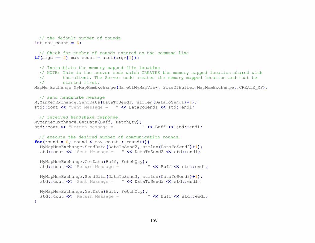
159
// the default number of rounds int max_count = 6; // Check for number of rounds entered on the command line if(argc == 2) max_count = atoi(argv[1]); // Instantiate the memory mapped file location // NOTE: This is the server code which CREATES the memory mapped location shared with // the client. The Server code creates the memory mapped location and must be // started first. MapMemExchange MyMapMemExchange(NameOfMyMapView, SizeOfBuffer,MapMemExchange::CREATE_MP); // send handshake message MyMapMemExchange.SendData(DataToSend1, strlen(DataToSend1)+1); std::cout << "Sent Message = " << DataToSend1 << std::endl; // received handshake response MyMapMemExchange.GetData(Buff, FetchQty); std::cout << "Return Message = " << Buff << std::endl; // execute the desired number of communication rounds. for(round = 0; round < max_count ; round++){ MyMapMemExchange.SendData(DataToSend2, strlen(DataToSend2)+1); std::cout << "Sent Message = " << DataToSend2 << std::endl; MyMapMemExchange.GetData(Buff, FetchQty); std::cout << "Return Message = " << Buff << std::endl; MyMapMemExchange.SendData(DataToSend3, strlen(DataToSend3)+1); std::cout << "Sent Message = " << DataToSend3 << std::endl; MyMapMemExchange.GetData(Buff, FetchQty); std::cout << "Return Message = " << Buff << std::endl; }

160
// send the "End" message. // This message will cause the client to shut down. MyMapMemExchange.SendData(DataToSend4, strlen(DataToSend4)+1); std::cout << "Sent Message = " << DataToSend4 << std::endl; // Return 0 to the Operating System return EXIT_SUCCESS; } /* ---------- end of function main ---------- */

161
/* * ===================================================================================== * * Filename: Client.cpp * * Description: This C++ client program is used to help demonstrate the use of * memory mapped files ( mmf ) in a Client / Server configuration. * * Version: 1.0 * Created: 6/13/2011 7:32:21 AM * Revision: none * Compiler: gcc or cl * Compilation Commands: * compile in Linux via a Cygwin command line prompt: * g++ -g -Wall -o Client.exe Client.cpp * * compile in Windows via Visual Studio 2008 command line prompt: * cl.exe /DWIN32 /EHsc /FeClient.exe Client.cpp * * Author: Jose E. Fadul (jef), * Company: AFIT * * Reference: This code is based on code written by David Maisonave. The original * source code, "InterprocessCommunicationWin32Example_client.cpp", is * located at http://code.axter.com. The complete url for this code is * http://code.axter.com/InterprocessCommunicationWin32Example_client.cpp * * ===================================================================================== */ #pragma warning(disable: 4786) #include <stdlib.h> #include <cstdlib>

162
#include <iostream> #include <windows.h> #include <string> /* * ===================================================================================== * Class: DataExchange * Description: Abstract Class used to define the main two functions required in * Exchanging Data, namely, SendData( ... ) and GetData( ... ). * ===================================================================================== */ class DataExchange { public: virtual ~DataExchange(){} virtual bool SendData(const char* Data, int Qty) = 0; virtual bool GetData(char* Data, int &Qty)=0; inline int GetErrorID(){return ErrorID;} protected: int ErrorID; }; /* * ===================================================================================== * Class: MapMemExchange * Description: An implementation Class of the DataExchange abstract class. * ===================================================================================== */ class MapMemExchange : public DataExchange { public: // A few constant enums used to help document the code, i.e., "OPEN_MP" is more

163
// descriptive than "0" and "CREATE_MP" is more descriptive than "1". enum OPEN_MODE{OPEN_MP, CREATE_MP}; enum EXCH_STAT{EMPTY_DATA, FETCH_DATA}; enum {DATA_INDEX = 1 + sizeof(int)}; // Notice the enum trick used here // to define a constant. This constant // specifies the data's starting memory // location. /* *-------------------------------------------------------------------------------------- * Class: MapMemExchange * Method: MapMemExchange :: MapMemExchange * Description: This method instantiates a MapMemExchange object given a name, size and * mode. * Inputs: const std::string &Name is the name of the memory mapped file. * int Size is the amount of memory to allocate to this * memory mapped filed. * OPEN_MODE mode is one of two desired memory mapped actions, * i.e., OPEN_MP to open a previously allocated * memory mapped located or CREATE_MP to allocate * memory for a memory mapped filed. *-------------------------------------------------------------------------------------- */ MapMemExchange(const std::string &Name, int Size, OPEN_MODE mode) :m_Name(Name), m_MapPtr(NULL), m_MapHandle(NULL), m_Size(Size), m_mode(mode) { m_MapHandle = (m_mode == CREATE_MP)? CreateFileMapping(INVALID_HANDLE_VALUE, NULL, PAGE_READWRITE, 0, m_Size + DATA_INDEX, m_Name.c_str()): OpenFileMapping(FILE_MAP_ALL_ACCESS, TRUE, m_Name.c_str()); if (m_MapHandle != INVALID_HANDLE_VALUE) {

164
m_MapPtr = (char*)MapViewOfFile(m_MapHandle, FILE_MAP_ALL_ACCESS, 0, 0, m_Size + DATA_INDEX); if (m_mode == CREATE_MP && m_MapPtr) { m_MapPtr[0] = EMPTY_DATA; memset(m_MapPtr+1, 0, sizeof(int)); } } } /* *-------------------------------------------------------------------------------------- * Class: MapMemExchange * Method: MapMemExchange :: SendData * Description: This is an implementation of the SendData virtual method defined in * the DataExchange abstract class. * Inputs: const char* Data is the character array written to the memory mapped * file location. * int Qty is the size of the given Data array. *-------------------------------------------------------------------------------------- */ bool SendData(const char* Data, int Qty) { if (!m_MapPtr) return false; // Spin lock used to wait until the memory mapped file location is free while(m_MapPtr[0] != EMPTY_DATA) { Sleep(0); } // copy the Data into the memory mapped filed location memcpy(m_MapPtr + DATA_INDEX, Data, Qty); // copy the Data array's size into the size memory mapped location memcpy(m_MapPtr +1, &Qty, sizeof(int));

165
// Set the data type / source value in memory to // 1 indicating that the data is from the server to the client or // 2 indicating that the data is from the client to the server. m_MapPtr[0] = FETCH_DATA+m_mode; // Now return true because all has gone well return true; } /* *-------------------------------------------------------------------------------------- * Class: MapMemExchange * Method: MapMemExchange :: GetData * Description: This is an implementation of the GetData virtual method defined in * the DataExchange abstract class. * Inputs: char* Data is the character array read in from the memory mapped * file location. * int &Qty is the size of the given read in Data array. *-------------------------------------------------------------------------------------- */ bool GetData(char* Data, int &Qty) { if (!m_MapPtr) return false; // spin lock used to wait for data // If the m_MapPtr[ 0 ] is 1 then the data is from the server to the client. // If the m_MapPtr[ 0 ] is 2 then the data is from the client to the server. while(m_MapPtr[0] != FETCH_DATA+(!m_mode)) { Sleep(0); } // read in the size of the data array memcpy(&Qty, m_MapPtr +1, sizeof(int)); // read in the data array memcpy(Data, m_MapPtr + DATA_INDEX, Qty); // Set the data type / source value in memory to

166
// 0 indicating that the memory location is free. m_MapPtr[0] = EMPTY_DATA; // return true indicating that the memory mapped data was read in successfully. return true; } /* *-------------------------------------------------------------------------------------- * Class: MapMemExchange * Method: MapMemExchange :: ~MapMemExchange * Description: This method is used to destroy the MapMemExchange object. * Inputs: None *-------------------------------------------------------------------------------------- */ ~MapMemExchange() { if (m_MapPtr) UnmapViewOfFile(m_MapPtr);; if (m_MapHandle) CloseHandle(m_MapHandle);; } private: const std::string m_Name; // name of the memory mapped filed location const int m_Size; // size of the memory mapped filed location char *m_MapPtr; // this is a pointer to the beginning of the memory mapped // file location HANDLE m_MapHandle; // This is a handle to the memory mapped file location const OPEN_MODE m_mode; // This is the mode used to access the memory mapped file // file location. };

167
/* * === FUNCTION ====================================================================== * Name: main * Description: This is the main entry point for the client program. * Inputs: int argc is not used * char *argv[] is not used * ===================================================================================== */ int main ( int argc, char *argv[] ) { // The name of the memory mapped file location const char NameOfMyMapView[] = "TestingAppCommunication"; // The amount of memory requested for the memory mapped file location const int SizeOfBuffer = 5000; // local variables used to hold the received message and its size char Buff[SizeOfBuffer]; int FetchQty = sizeof(Buff); // messages sent to server from client const char* DataToSend1 = "Bush"; const char* DataToSend2 = "Response1"; const char* DataToSend3 = "Response2"; const char* DataToSend4 = "Unknown"; // Instantiate the memory mapped file location // NOTE: This is the client code which OPEN'S a previous created memory mapped location. // The Server code creates the memory mapped location. MapMemExchange MyMapMemExchange(NameOfMyMapView, SizeOfBuffer,MapMemExchange::OPEN_MP); // wait for data from the server MyMapMemExchange.GetData(Buff, FetchQty); // echo what was recieved from the server std::cout << "Received Message = " << Buff << std::endl;

168
// Determine the proper response // by checking the first character's value in the received message. while(Buff[0] != 'E'){ // check for "End" message switch(Buff[0]){ case 'G': // repond to "George" message. MyMapMemExchange.SendData(DataToSend1, strlen(DataToSend1)+1); std::cout << "Sent Message = " << DataToSend1 << std::endl; break; case 'R': // repond to "Request" message. MyMapMemExchange.SendData(DataToSend2, strlen(DataToSend2)+1); std::cout << "Sent Message = " << DataToSend2 << std::endl; break; case 'A': // respond to "Action" message. MyMapMemExchange.SendData(DataToSend3, strlen(DataToSend3)+1); std::cout << "Sent Message = " << DataToSend3 << std::endl; break; default: // respond to unknown messages. MyMapMemExchange.SendData(DataToSend4, strlen(DataToSend4)+1); std::cout << "Sent Message = " << DataToSend4 << std::endl; break; } // wait for data from the server MyMapMemExchange.GetData(Buff, FetchQty); // echo what was recieved from the server std::cout << "Received Message = " << Buff << std::endl; } // Return 0 to the Operating System return EXIT_SUCCESS; } /* ---------- end of function main ---------- */

169
Appendix F Example R Statistical language and MatLab scripts
# # ===================================================================================== # # Filename: Example_R_Script.r # # Description: This R script reads in two ASCII data files and # produces three plots # (Histogram, Quantile-Quantile plot and Bar plot) # # Version: 1.0 # Created: 4/27/2011 9:55:13 AM # Revision: none # Compiler: R Statistical Program # # Author: Jose E. Fadul (jef), # Company: AFIT # # Note: This example is based on an example I found on the internet a while ago. # # Usage: 1) Open an R term or R gui window # 2) Change the process working directory (pwd) to # the directory containing the data files with "setwd()" function or # with equivalent gui menu option # 3) Copy and paste this file into the R window # /* The R commands will execute and create the 3 plots*/ # # ===================================================================================== #

170
# # === FUNCTION ======================================================================== # Name: error.bar # Description: Used to add error bars to pre-existing bar plot # Author: Unknown, i.e. I did not create this function. # I found it on the internet. # Inputs: x a vector identifying the x coordinates of the error bars # y a vector identifying the y coordinates of the error bars # upper a vector identifying the upper y coordinate delta amounts # i.e., "upper y" coordinate = y + upper # lower a vector identifying the lower y coordinate delta amounts # i.e., "lower y" coordinate = y + lower # default is upper vector values # length a single value used for the error bar's width, # default is 0.1 # ... additional parameter values are passed to the arrows function # ===================================================================================== # error.bar <- function(x, y, upper, lower=upper, length=0.1,...){ if(length(x) != length(y) | length(y) !=length(lower) | length(lower) != length(upper)) stop("vectors must be same length") arrows(x,y+upper, x, y-lower, angle=90, code=3, length=length, ...) } # # === READ IN DATA ==================================================================== # # use the read.table function to read in the two data files into data frames y and y1

171
# # data files contain space delimined data, such as: # # -0.19040E-01 -0.21490E-01 -0.24941E-01 # -0.21542E-01 -0.24642E-01 -0.24760E-01 # -0.21684E-01 -0.23224E-01 -0.26115E-01 # -0.20510E-01 -0.23618E-01 -0.25179E-01 # -0.19005E-01 -0.20917E-01 -0.23241E-01 # -0.22868E-01 -0.24729E-01 -0.26674E-01 # -0.19664E-01 -0.22577E-01 -0.27032E-01 # -0.21500E-01 -0.23575E-01 -0.28163E-01 # -0.18803E-01 -0.21217E-01 -0.23994E-01 # # ===================================================================================== # y <- read.table("last_values_original_5_10_15.txt") y1 <- read.table("last_values_trusted_5_10_15.txt") # # === PROCESS DATA ==================================================================== # # Convert data values from Per Unit (PU) to Hertz (Hz) and # from a data frame to a matrix. # # Calculate the "mean" and "standard deviation" values for each column using # the apply function, i.e., 2nd dimension of the matrix. # # Create a 2 by 3 matrix of "mean values" for the bar plot. # # Create a 2 by 3 matrix of "95% confidence interval values" for the error bars # that are added to the bar plot.

172
# # ===================================================================================== # y <- 60*(1 + as.matrix(y)) y1 <- 60*(1 + as.matrix(y1)) y.means <- apply(y,2,mean) y.sd <- apply(y,2,sd) y1.means <- apply(y1,2,mean) y1.sd <- apply(y1,2,sd) yy <- matrix(c(y.means,y1.means),2,3,byrow=TRUE) ee <- matrix(c(y.sd,y1.sd),2,3,byrow=TRUE)*1.96/sqrt(36) # # === BAR PLOT ======================================================================== # # Create bar plot and store the x coordinate values in "barx" # # See the barplot function in the help documentation for parameter details # The help is accessed from within R with "?barplot" or "??barplot" # # Add error bars to the bar plot # # Add a title to the bar plot # # Add a legend to the bar plot # # Add a box around the bar plot #
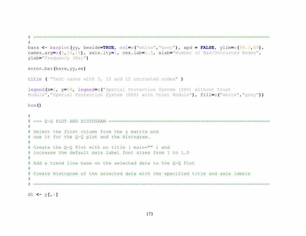
173
# ===================================================================================== # barx <- barplot(yy, beside=TRUE, col=c("white","grey"), xpd = FALSE, ylim=c(58.3,59), names.arg=c(5,10,15), axis.lty=1, cex.lab=1.5, xlab="Number of Bad/Untrusted Nodes", ylab="Frequency (Hz)") error.bar(barx,yy,ee) title ( "Test cases with 5, 10 and 15 untrusted nodes" ) legend(x=1, y=59, legend=c("Special Protection System (SPS) without Trust Module","Special Protection System (SPS) with Trust Module"), fill=c("white","grey")) box() # # === Q-Q PLOT AND HISTOGRAM ========================================================== # # Select the first column from the y matrix and # use it for the Q-Q plot and the Histogram. # # Create the Q-Q Plot with no title ( main="" ) and # increase the default axis label font sizes from 1 to 1.5 # # Add a trend line base on the selected data to the Q-Q Plot # # Create Histogram of the selected data with the specified title and axis labels # # ===================================================================================== d1 <- y[,1]

174
qqnorm(d1, main = "", cex.lab=1.5) qqline(d1) hist(d1, main = "Histogram of simulation data with 5 untrusted Nodes", cex.lab=2, ylab = "Number of Observations", xlab = "Frequency in Hertz") # # === END OF FILE ===================================================================== # vim:tw=100:ts=4:ft=R:norl:lbr: # =====================================================================================
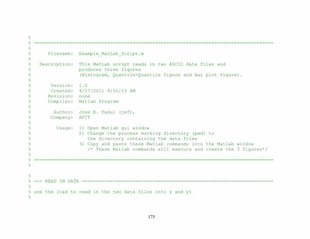
175
% % ===================================================================================== % % Filename: Example_MatLab_Script.m % % Description: This MatLab script reads in two ASCII data files and % produces three figures % (Histogram, Quantile-Quantile figure and Bar plot figure). % % Version: 1.0 % Created: 4/27/2011 9:55:13 AM % Revision: none % Compiler: Matlab Program % % Author: Jose E. Fadul (jef), % Company: AFIT % % Usage: 1) Open Matlab gui window % 2) Change the process working directory (pwd) to % the directory containing the data files % 3) Copy and paste these Matlab commands into the Matlab window % /* These Matlab commands will execute and create the 3 figures*/ % % ===================================================================================== % % % === READ IN DATA ==================================================================== % % use the load to read in the two data files into y and y1 %

176
% data files contain space delimined data, such as: % % -0.19040E-01 -0.21490E-01 -0.24941E-01 % -0.21542E-01 -0.24642E-01 -0.24760E-01 % -0.21684E-01 -0.23224E-01 -0.26115E-01 % -0.20510E-01 -0.23618E-01 -0.25179E-01 % -0.19005E-01 -0.20917E-01 -0.23241E-01 % -0.22868E-01 -0.24729E-01 -0.26674E-01 % -0.19664E-01 -0.22577E-01 -0.27032E-01 % -0.21500E-01 -0.23575E-01 -0.28163E-01 % -0.18803E-01 -0.21217E-01 -0.23994E-01 % % ===================================================================================== % y = load('last_values_original_5_10_15.txt'); y1 = load('last_values_trusted_5_10_15.txt'); % % === PROCESS DATA ==================================================================== % % Convert data values from Per Unit (PU) to Hertz (Hz). % % Calculate the "mean" and "standard deviation" values for each column using % the mean and std functions. % % Create a 3 by 2 matrix of "mean values" for the bar plot. % % Create a 3 by 2 matrix of "95% confidence interval values" for the error bars % that are added to the bar plot. % % =====================================================================================

177
% y = 60*(1 + y); y1 = 60*(1 + y1); y_means = mean(y,1); y_sd = std(y,1,1); y1_means = mean(y1,1); y1_sd = std(y1,1,1); yy = [y_means;y1_means]'; ee = [y_sd;y1_sd]'.*1.96/sqrt(36); % % === BAR PLOT ======================================================================= % % Create bar figure % % See the bar function in the help documentation for parameter details % The help is accessed from within Matlab with "help bar" % % Set the axis limits with the axis function % % store the x coordinate values in "barx" % % Add error bars to the bar plot % % Add title and axis labels using the figure's gui editor and double clicking on the item % you want to change. %
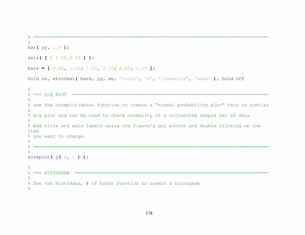
178
% ===================================================================================== % bar( yy, 1.0 ); axis( [ 0 4 58.2 59 ] ); barx = [ 0.85, 1.15; 1.85, 2.15; 2.85, 3.15 ]; hold on, errorbar( barx, yy, ee, 'color', 'k', 'linestyle', 'none' ), hold off % % === Q-Q PLOT ======================================================================= % % use the normplot(data) function to create a "normal probability plot" this is similar a % Q-Q plot and can be used to check normality of a colloected sample set of data % % Add title and axis labels using the figure's gui editor and double clicking on the item % you want to change. % % ===================================================================================== % normplot( y( :, 1 ) ); % % === HISTOGRAM ====================================================================== % % Use the hist(data, # of bins) function to create a histogram %

179
% Add title and axis labels using the figure's gui editor and double clicking on the item % you want to change. % % ===================================================================================== % hist( y( :,1 ), 7 ); % % === END OF FILE ==================================================================== % vim:tw=100:ts=4:ft=Matlab:norl:lbr: % =====================================================================================

180
% % ===================================================================================== % % Filename: Example_MatLab_Script_v2.m % % Description: This MatLab script reads in two ASCII data files and % produces three figures % (Histogram, Quantile-Quantile figure and Bar plot figure). % % Version: 2.0 % Created: 4/27/2011 5:00:00 PM % Revision: none % Compiler: Matlab Program % % Author: Jose E. Fadul (jef), % Company: AFIT % % Usage: 1) Open Matlab gui window % 2) Change the process working directory (pwd) to % the directory containing the data files % 3) Copy and paste these Matlab commands into the Matlab window % /* These Matlab commands will execute and create the 3 figures*/ % % ===================================================================================== % % % === READ IN DATA ==================================================================== % % use the load to read in the two data files into y and y1 %

181
% data files contain space delimined data, such as: % % -0.19040E-01 -0.21490E-01 -0.24941E-01 % -0.21542E-01 -0.24642E-01 -0.24760E-01 % -0.21684E-01 -0.23224E-01 -0.26115E-01 % -0.20510E-01 -0.23618E-01 -0.25179E-01 % -0.19005E-01 -0.20917E-01 -0.23241E-01 % -0.22868E-01 -0.24729E-01 -0.26674E-01 % -0.19664E-01 -0.22577E-01 -0.27032E-01 % -0.21500E-01 -0.23575E-01 -0.28163E-01 % -0.18803E-01 -0.21217E-01 -0.23994E-01 % % ===================================================================================== % y = load('last_values_original_5_10_15.txt'); y1 = load('last_values_trusted_5_10_15.txt'); % % === PROCESS DATA ==================================================================== % % Convert data values from Per Unit (PU) to Hertz (Hz). % % Create a single data matrix, i.e., observations by treatments. In this case 36 by 6. % % get the number of observations and the number of treatments via the size function. % % transform the data matrix into a vector. % % Assign groups labels to the data values. % % Calculate the "mean" and "confidence interval" values for each column using
182
% the grpstats functions. % % Create a 3 by 2 matrix of "95% confidence interval values" for the error bars % that are added to the bar plot. % % Create a 3 by 2 matrix of "mean values" for the bar plot. % % ===================================================================================== % y = 60*(1 + y); y1 = 60*(1 + y1); data = [ y, y1 ]; [ M, N ] = size( data ); data = reshape( data, M*N, 1 ); A = ones( M, 1 ); B = ( 1:N )*5; groups = reshape( A*B, M*N, 1 ); [ M, CI, levels ] = grpstats( data, groups, {'mean', 'meanci', 'gname' }); CI = reshape( CI( :,2 )-M, N/2, 2 ); M = reshape( M, N/2, 2 ); %

183
% === BAR PLOT ======================================================================= % % Create bar figure % % See the bar function in the help documentation for parameter details % The help is accessed from within Matlab with "help bar" % % Set the axis limits with the axis function % % store the x coordinate values in "barx" % % Add error bars to the bar plot % % Add title and axis labels using the figure's gui editor and double clicking on the item % you want to change. % % ===================================================================================== % bar( M, 1.0 ); axis( [ 0 4 58.2 59.0 ] ); barx = [ ( 1:N/2 )-0.15; ( 1:N/2 )+0.15 ]'; hold on, errorbar( barx, M, CI, 'color', 'k', 'linestyle', 'none' ), hold off % % === Q-Q PLOT ======================================================================= %

184
% use the normplot(data) function to create a "normal probability plot" this is similar a % Q-Q plot and can be used to check normality of a colloected sample set of data % % Add title and axis labels using the figure's gui editor and double clicking on the item % you want to change. % % ===================================================================================== % normplot( y( :, 1 ) ); % % === HISTOGRAM ====================================================================== % % Use the hist(data, # of bins) function to create a histogram % % Add title and axis labels using the figure's gui editor and double clicking on the item % you want to change. % % ===================================================================================== % hist( y( :,1 ), 7 ); % % === END OF FILE ==================================================================== % vim:tw=100:ts=4:ft=Matlab:norl:lbr: % =====================================================================================

185
Appendix G PSS/E and NS2 Automation batch files
Figure 52. Sequence diagram of the simulation automation batch file processes
The fully commented batch file scripts and C++ file source code provided in this appendix are intended to help future
student automate their simulation and data collection efforts, as well as, gain some understanding into how the simulations were
run in the PSS/E power simulator experiments, see Figure 52.
Start a separate NS2 Process
Create two text files to terminate the NS2 process
replace_FF_win_version.exeCall_PSSPLT.bat remove_headers.bat R_cmd.batUser Run_Seeds.Bat main.bat ns2_driver.bat Call_PSSDS4.bat remove_headers_from_load_flow_file.bat
186
:: ::===================================================================================== :: :: Filename: run_seeds.bat :: :: Description: This MSDOS batch file uses the random seed values contained in :: "seeds.txt" to execute experiments via calls to "main.bat". :: :: Each line in "seeds.txt" is read into variable 'a' and passed to :: "main.bat" as a command line parameter. :: :: Hence, "main.bat" is called once for each seed value in "seeds.txt". :: :: Version: 1.0 :: Created: 6/10/2011 8:46:13 AM :: Revision: none :: Compiler: none :: :: Author: Jose E. Fadul (jef), :: Company: AFIT :: ::===================================================================================== :: @echo off FOR /F %%a IN (seeds.txt) DO call main.bat %%a

187
:: ::===================================================================================== :: :: Filename: main.bat :: :: Description: This MSDOS batch file executes one simulation Run of PSS/E with :: NS2 network support. :: :: ( 1 ) calls "ns2_driver.bat", which spawns an NS2 process. :: :: ( 2 ) waits 8 seconds before calling "Call_PSSDS4.bat". This delay :: allows NS2 to remove temporary files and initiate the power :: grid network nodes/links required for simulation. :: :: ( 3 ) calls "Call_PSSDS4.bat", which creates and executes a PSS/E :: simulation script. This simulation script generates the :: desired data in PSS/E binary format and converts it to ascii :: format via "Call_PSSPLT.bat". The resulting ascii text file :: is further processed to removed extraneous header data. :: :: ( 4 ) create two additional EPOCHS text files, "in_out" and "in_go", :: to enable NS2 to end gracefully. :: :: NOTE: The EPOCHS communication protocol between NS2 and PSS/E :: has NS2 waiting for a response when PSS/E terminates :: its execution. The two generated fies provide NS2 the :: response it is waiting for and enables NS2's graceful :: termination. :: :: ( 5 ) wait 2 seconds before running the next simulation or :: terminating.

188
:: :: inputs: <optional> random seed value :: If a random seed value is provided, then it is used in the output :: filenames generated by "Call_PSSDS4.bat" and used in NS2 to :: initialize the random number generator via "ns2_driver.bat". :: If no random seed value is provided, then a default value of "12345" :: is used to initialize the NS2 random number generator and no seed :: value is included in the generated output filenames. :: :: NOTE: if a random seed value is provided, then it is stored in :: command line argument variable '1' and accessed via '%1'. :: :: Version: 1.0 :: Created: 6/10/2011 8:44:34 AM :: Revision: none :: Compiler: none :: :: Author: Jose E. Fadul (jef), :: Company: AFIT :: ::===================================================================================== :: :: :: Calls MSDOS batch file "ns2_driver.bat" with random seed value '%1'. This batch file :: spawns a new NS2 process, which interacts with PSS/E via the EPOCHS RunTime Interface :: protocol. :: :: NOTE: if no random seed value is provided, then '%1' is empty and NS2 uses "12345" :: as a default random seed value.

189
:: call ns2_driver.bat %1 :: :: The following two lines are used to pause this "main.bat" process for 8 seconds. :: This 8 second delay provides NS2 time to remove temporary file and setup the :: power grid network nodes/links for the simulation run. :: :: NOTE: The Windows system initially used for development does not have the :: batch file sleep command, hence the uses of this ping trick. @ping 127.0.0.1 -n 2 -w 1000 > nul @ping 127.0.0.1 -n 6 -w 1000 > nul :: :: Calls MSDOS batch file "Call_PSSDS4.bat" with random seed value '%1'. This batch file :: credates and executes a PSS/E simulation script, which interacts with NS2 via the :: EPOCHS RunTime Interface protocol. :: :: NOTE: if no random seed value is provided, then '%1' is empty and PSS/E uses "" :: as a default random seed value, i.e., no seed value is appended to output :: filenames. :: call Call_PSSDS4.bat %1 :: :: The following two lines create the "in_out" and "in_go" EPOCHS files. When PSS/E's :: simulation run terminates, NS2 is waiting for a response via EPOCHS. This response :: is provided by these two generated files. Once, NS2 receives this response its :: terminates gracefully. ::
190
:: NOTE: The order of the following two line is important. The data file, "in_out", :: must be created before the guard file, "in_go". The guard file is used to :: inform NS2 that the response data file is ready for NS2 to use. :: copy c:\ken\swap\close_pipe.txt c:\ken\swap\in_out >NUL copy c:\ken\swap\close_pipe_in_go.txt c:\ken\swap\in_go >NUL :: :: An alternative method to create the two EPOCHS files is provided in the following :: three commented lines. Feel free to choose your desired method. :: ::echo AGENTS>c:\ken\swap\in_out ::echo END_FILE>>c:\ken\swap\in_out ::echo go>c:\ken\swap\in_go :: :: Wait an additional 2 seconds before running the the next simulation or terminating. :: This gives the Operating System and NS2 a chance to complete all simulation :: terminating tasks, such as, exiting NS2, terminating the spawned NS2 process and :: closing all simulation related intermediate and data files. :: @ping 127.0.0.1 -n 1 -w 1000 > nul @ping 127.0.0.1 -n 1 -w 1000 > nul :: :: force one more command line carriage return to insure all processes have :: successfully terminated. :: echo.

191
:: ::===================================================================================== :: :: Filename: ns2_driver.bat :: :: Description: This MSDOS batch file spawns an NS2 process, which interacts with :: PSS/E via the EPOCHS RunTime Interface protocol. :: :: inputs: <optional> random seed value :: If a random seed value is provided, then it is used in NS2 to :: initialize the random number generator. If no random seed value is :: provided, then a default value of "12345" is used to initialize the :: NS2 random number generator. :: :: NOTE: if a random seed value is provided, then it is stored in :: command line argument variable '1' and accessed via '%1'. :: :: Version: 1.0 :: Created: 6/10/2011 8:44:49 AM :: Revision: none :: Compiler: none :: :: Author: Jose E. Fadul (jef), :: Company: AFIT :: ::===================================================================================== :: :: :: The command line start command and "cmd.exe" program are used to spawn the new :: NS2 process.

192
:: :: The start command specifies the environment variables and the process working :: directory used in the newly spawned process, via command line switches /I and /D, :: respectively. :: :: The "cmd.exe" program executes the NS2 executable within the newly spawned process :: environment. The command line switch /c causes the newly spawned process to :: terminate when NS2 terminates. :: :: The NS2 executable is called with a simulation script file, written in Object Tool :: Command Language (Otcl, also known as tcl). This tcl script has one optional input :: command line parameter, which is the random seed value. If ns2_driver.bat is called :: with a random seed value, then this value is assigned to command line argument :: variable '1' and provided to the tcl script as a parameter via '%1'. :: :: NOTE: if no random seed value is provided, then '%1' is empty and tcl script uses :: "12345" as a default random seed value to initialize NS2's random number :: generator. :: start /I /Dc:\ken\swap cmd.exe /c C:/cygwin/home/AFIT/ns-allinone-2.29_psse/ns-2.29/ns.exe nscript_20101208_0945.tcl %1

193
:: ::===================================================================================== :: :: Filename: Call_PSSDS4.BAT :: :: Description: This MSDOS batch files creates and executes a PSS/E simulation :: script, which interfaces with NS2 via EPOCHS RunTime Interface :: protocol. This simulation script generates the desired data in :: PSS/E binary format and converts it to ascii format via :: "Call_PSSPLT.bat". The resulting ascii text file is further :: processed to removed extraneous header data. :: :: ( 1 ) Auto echoing of commands is turned off :: :: ( 2 ) Append PSS/E binary and library file directories to the :: current environment's PATH variable. This insures that :: the PSS/E executable, and its supporting binary and library :: files, are found by the Operating System. :: :: ( 3 ) The current system date and time are stored in MSDOS batch :: file variables 'd' and 't', respectively, and accessed via :: '%d%' and '%t%'. :: :: NOTE: Notice how these variables are wrapped in :: percent signs, i.e., two percent signs are used to access :: the variable's value. :: :: Formats: :: The date format used is year month day. :: For example, July 4, 2011 is represented by 20110704 ::

194
:: The time format used is hour minutes. :: For example, half past eight AM is represented :: by 0830 and 4:30:15 PM is represented by 1630 :: :: ( 4 ) Provide command line feedback by echoing :: "Your PATH is now set to run PSS/E-30 programs!" :: :: ( 5 ) Set the current directory as the process working directory. :: :: ( 6 ) Create the PSS/E simulation script. :: :: ( 7 ) Execute the created PSS/E simulation script. :: :: ( 8 ) <optional> delete the created PSS/E simulation script. :: :: ( 9 ) Wait 4 seconds for the output data files to be created :: and available for use by the R statistical program. :: :: ( 10 ) <optional> If the PSS/E simulation's data file exist, :: then use it to generate a graph in PDF file format via :: the R statistical program. :: :: inputs: <optional> random seed value :: If a random seed value is provided, then it is used in the output :: filenames generation commands. If no random seed value is provided, :: then no seed value is included in the generated output filenames. :: :: NOTE: if a random seed value is provided, then it is stored in :: command line argument variable '1' and accessed via '%1'. :: :: Version: 1.0

195
:: Created: 6/10/2011 8:41:47 AM :: Revision: none :: Compiler: none :: :: Author: Jose E. Fadul (jef), :: Company: AFIT :: ::===================================================================================== :: :: :: The following command disables the auto-echoing of batch file commands. :: @echo OFF :: :: The following set command is used to append PSS/E binary and library file :: directories to the current path environment variable. :: SET PATH=C:\PROGRA~1\PTI\PSSE30\PSSBIN;C:\PROGRA~1\PTI\PSSE30\PSSLIB;%PATH% :: :: The following 16 lines are used to get and format the system's date and time :: values. The current system date and time values are stored in MSDOS batch :: file variables 'd' and 't', respectively, and accessed via '%d%' and '%t%'. :: :: NOTE: Notice how these variables are wrapped in percent signs, :: i.e., two percent signs are used to access the variable's value. :: :: Formats: The date format used is year month day. :: For example, July 4, 2011 is represented by 20110704

196
:: :: The time format used is hour minutes. :: For example, half past eight AM is represented by 0830 :: and 4:30:15 PM is represented by 1630 :: for /f "eol=; tokens=1,2,3,4,5* delims=/ " %%u in ('date /t') do set d=%%x%%v%%w for /f "eol=; tokens=1,2,3,4* delims=: " %%u in ('time /t') do ( set t=%%u%%v set c=%%w ) if "%c%" == "PM" ( if "%t:~0,1%" == "0" (set /A t=%t:~1,3% + 1200) if "%t:~0,2%" == "10" (set /A t=%t% + 1200) if "%t:~0,2%" == "11" (set /A t=%t% + 1200) ) if "%c%" == "AM" ( if "%t:~0,2%" == "12" (set t=00%t:~2,2%) ) :: :: The following three lines provide command line feedback that all is well. :: echo. echo Your PATH is now set to run PSS/E-30 programs! echo. :: :: This command sets the current batch file's current directory is the :: process working directory.

197
:: cd %~dp0 :: :: The following echo commands are used to create the PSS/E simulation script. :: This simulation script calls batch files "remove_headers_from_load_flow_file.bat" :: and "Call_PSSPLT.bat" via PSS/E's system command. :: :: NOTE: modifying these echo commands is not trivial and requires knowledge of the :: desired output file template. This template can be created within PSS/E :: via its menu functions. See PSS/E manual for instructions on creating an :: input 'Response file' for command line automation, i.e., look in the :: users manual, "USER.PDF", for information concerning 'program automation' :: and 'Response file' (file type idv). :: echo MENU,OFF /* FORCE MENU TO CORRECT STATUS>pssds4_test.idv echo LOFL>>pssds4_test.idv echo CASE>>pssds4_test.idv echo 50c.sav>>pssds4_test.idv echo OPEN>>pssds4_test.idv echo 2 0 ^1>>pssds4_test.idv echo 50_Load_Flow_%d%_%t%_%1.dat>>pssds4_test.idv echo RTRN,FACT>>pssds4_test.idv echo DYRE>>pssds4_test.idv echo 50.dyr>>pssds4_test.idv echo. >>pssds4_test.idv echo. >>pssds4_test.idv echo ,,,>>pssds4_test.idv echo ALTR>>pssds4_test.idv echo ^6>>pssds4_test.idv echo Y>>pssds4_test.idv
198
echo 50,,,,>>pssds4_test.idv echo Y>>pssds4_test.idv echo ,,0.002,,,>>pssds4_test.idv echo N>>pssds4_test.idv echo N>>pssds4_test.idv echo ^0>>pssds4_test.idv echo ^0>>pssds4_test.idv echo CHAN>>pssds4_test.idv echo , , ,>>pssds4_test.idv echo 12>>pssds4_test.idv echo 110>>pssds4_test.idv echo. >>pssds4_test.idv echo ^0>>pssds4_test.idv echo MSTR>>pssds4_test.idv echo 50_results_%d%_%t%_%1.out>>pssds4_test.idv echo MRUN>>pssds4_test.idv echo 0.0,1,1,^0>>pssds4_test.idv echo BAT_DIST_BRANCH_FAULT 1 25 "1" 1 500.00 0.0000 -0.20000E+10 ;>>pssds4_test.idv echo MRUN>>pssds4_test.idv echo 0.15,1,1,^0>>pssds4_test.idv echo BAT_DIST_BRANCH_TRIP 1 25 "1" ;>>pssds4_test.idv echo MRUN>>pssds4_test.idv echo 0.1800,1,1,^0>>pssds4_test.idv :: :: Uncomment the following lines when running psse without ns2 :: :: echo BAT_POWERFLOWMODE ;>>pssds4_test.idv :: echo BAT_PLANT_DATA, 93, , , ;>>pssds4_test.idv :: echo BAT_MACHINE_DATA, 93, "1", 0, , , , ,>>pssds4_test.idv :: echo , , , , , , , ,>>pssds4_test.idv
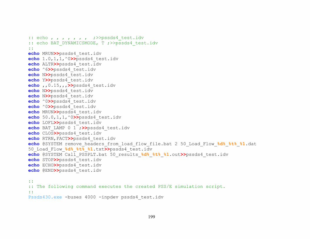
199
:: echo , , , , , , , ;>>pssds4_test.idv :: echo BAT_DYNAMICSMODE, T ;>>pssds4_test.idv :: echo MRUN>>pssds4_test.idv echo 1.0,1,1,^0>>pssds4_test.idv echo ALTR>>pssds4_test.idv echo ^6>>pssds4_test.idv echo N>>pssds4_test.idv echo Y>>pssds4_test.idv echo ,,0.15,,,>>pssds4_test.idv echo N>>pssds4_test.idv echo N>>pssds4_test.idv echo ^0>>pssds4_test.idv echo ^0>>pssds4_test.idv echo MRUN>>pssds4_test.idv echo 50.0,1,1,^0>>pssds4_test.idv echo LOFL>>pssds4_test.idv echo BAT_LAMP 0 1 ;>>pssds4_test.idv echo CLOS>>pssds4_test.idv echo RTRN,FACT>>pssds4_test.idv echo @SYSTEM remove_headers_from_load_flow_file.bat 2 50_Load_Flow_%d%_%t%_%1.dat 50_Load_Flow_%d%_%t%_%1.txt>>pssds4_test.idv echo @SYSTEM Call_PSSPLT.bat 50_results_%d%_%t%_%1.out>>pssds4_test.idv echo STOP>>pssds4_test.idv echo ECHO>>pssds4_test.idv echo @END>>pssds4_test.idv :: :: The following command executes the created PSS/E simulation script. :: Pssds430.exe -buses 4000 -inpdev pssds4_test.idv
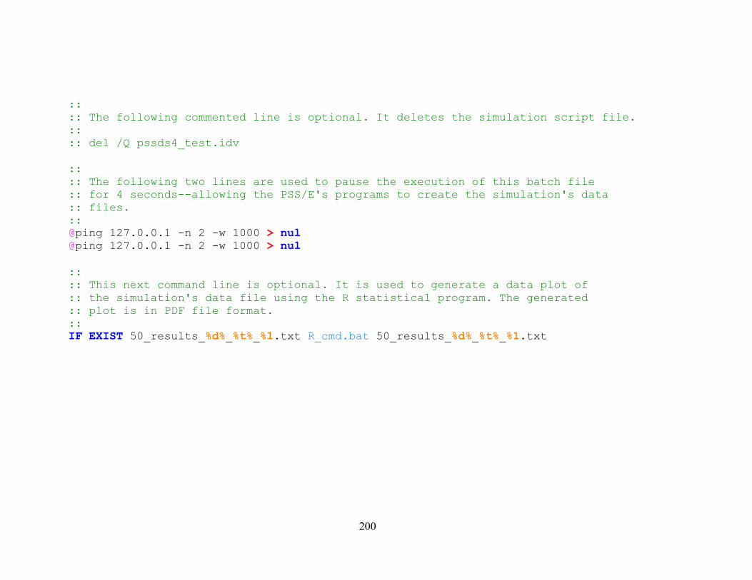
200
:: :: The following commented line is optional. It deletes the simulation script file. :: :: del /Q pssds4_test.idv :: :: The following two lines are used to pause the execution of this batch file :: for 4 seconds--allowing the PSS/E's programs to create the simulation's data :: files. :: @ping 127.0.0.1 -n 2 -w 1000 > nul @ping 127.0.0.1 -n 2 -w 1000 > nul :: :: This next command line is optional. It is used to generate a data plot of :: the simulation's data file using the R statistical program. The generated :: plot is in PDF file format. :: IF EXIST 50_results_%d%_%t%_%1.txt R_cmd.bat 50_results_%d%_%t%_%1.txt

201
:: ::===================================================================================== :: :: Filename: remove_headers_from_load_flow_file.bat :: :: Description: This MSDOS batch files removes extraneous header information for :: the output load flow file created by PSS/E's program. :: :: Inputs: <Required> <column headings number> :: The column heading number control how many heading lines :: are used as the column headings. :: :: NOTE: This number is normally 0, 2 or 3, where 0 :: indicates that no column heading is needed :: (i.e., just data without and column headings) and :: a 2 or 3 indicates that a two or three lines are :: desired for column headings in the output. :: :: <Required> <ASCII text data input filename> :: The input data filename specifies the file with the :: ASCII text with the extra heading information. :: :: <Optional> <ASCII Text data output filename> :: This output data filename indicates that the process :: data file should be saved in the current directory with :: the given output filename. :: :: If the output filename is omitted, then the processed :: data is sent to the standard output device, i.e., stdout. :: This is normally the command line terminal. ::

202
:: :: Version: 1.0 :: Created: 6/10/2011 8:45:55 AM :: Revision: none :: Compiler: none :: :: Author: Jose E. Fadul (jef), :: Company: AFIT :: ::===================================================================================== :: :: :: The following command disables the auto-echoing of batch file commands. :: @echo off :: :: The following command enables extra batch file set command features, such as, :: mathematical calculations in conjunction with batch variable value assignments. :: setlocal enabledelayedexpansion :: :: The following two lines check for the required parameters. :: :: If the parameters are missing goto the usage label and provide some basic usage :: information. :: :: If the parameters are present then continue. ::

203
if [%1] == [] goto usage if [%2] == [] goto usage :: :: The following two lines are used to remove the form feed ( FF ) characters from :: the input data file. :: :: The executable program searches for the FF character and replaces it with an :: end of line (eol) character, namely a printf '\n' character. The processed :: files is saved as a a tmp file during processing. After processng the tmp file :: replaces the input data file. :: replace_FF_win_version.exe %2 %2.tmp move %2.tmp %2 :: :: Set the column header counter variable to zero. :: SET /a counter=0 :: :: If the third command line variable is omitted, then send processed data to :: standard output device, i.e., stdout which is normally the command line terminal. :: if [%3] == [] goto stdout :: :: If the output data filename exist, then delete it without any warning. :: del /Q %3 2>NUL

204
:: :: The following FOR loop extracts the desired number of column heading lines from :: the given input data file to the given output data file. :: FOR /F "skip=4 usebackq tokens=* delims=" %%i in (%2) do ( if "!counter!"=="%1" goto next1 echo %%i >> %3 SET /a counter+=1 ) :: :: The following goto command should never be reach under normal operation, :: but included to catch possible errors within the above FOR loop command. :: goto next1 :: :: The following line is a goto target label, used to redirect the batch :: file's execution flow. :: :: This particular label marks the beginning of the execution path when no :: output filename is given. :: :stdout :: :: The following FOR loop extracts the desired number of column heading lines from :: the given input data file to the standard output device, i.e., stdout which is :: normally the command line terminal. :: FOR /F "skip=4 usebackq tokens=* delims=" %%i in (%2) do (

205
if "!counter!"=="%1" goto next2 echo %%i SET /a counter+=1 ) :: :: The following goto command should never be reach under normal operation, :: but included to catch possible errors within the above FOR loop command. :: goto next2 :: :: The following line is a goto target label, used to redirect the batch :: file's execution flow. :: :: This particular label marks the beginning of the usage information provided :: to the user to help them use this batch file correctly. :: :usage echo. echo Usage: remove_headers.bat ^<column heading line number^> ^<input_filename^> [^<output_filename^>] echo. echo note: column heading line number is off-set by 4, i.e. for the fifth file line enter 1. echo you normally want this number to be 0 or 2 or 3. echo. :: :: The following goto statement terminates this batch file's execution by :: going to the end of this file. :: goto exit

206
:: :: This is legacy comment information created and referenced during development. :: rem example: remove_headers_from_load_flow_file.bat 0 50_Load_Flow_results_20100930_1135.DAT 50_Load_Flow_results_20100930_1135.txt rem rem OR rem rem remove_headers_from_load_flow_file.bat 2 50_Load_Flow_results_20100930_1135.DAT 50_Load_Flow_results_20100930_1135.txt rem rem OR rem rem remove_headers_from_load_flow_file.bat 3 50_Load_Flow_results_20100930_1135.DAT 50_Load_Flow_results_20100930_1135.txt rem rem The column heading line number specifies which line is the column heading line. rem This line number is off-set by 4, i.e. for the fifth file line enter a value of 1. rem A value of zero indicates that no column heading is desired in the output.
:: :: The following line is a goto target label, used to redirect the batch :: file's execution flow. :: :: This particular label marks the continuation of the execution path when an :: output filename is given. :: :next1 :: :: The following multi-piped findstr commands are used to extract the data values from :: the given input data file and appends them to the given output data file. :: :: The findstr command perform the following string processing actions: :: :: ( 1 ) findstr /v /i "pti identification IEEE Channel TIME" %2 :: This findstr command removes all the lines containing

207
:: any one of the given words from the input data file. Hence, the lines without :: any of these given words is piped to the next findstr command. :: :: ( 2 ) findstr /R /V "^.$" :: This command removes all the lines that contain only one character. The lines :: with 2 or more characters, as well as, blank lines are piped to the next :: findstr command. :: :: ( 3 ) findstr /R /V "^$" :: This final findstr command removes all the blank lines from the input data. :: Hence only the data lines with 2 or more characters are appended to the given :: output data file. :: findstr /v /i "pti identification IEEE FROM BASKV" %2 | findstr /R /V "^.$" | findstr /R /V "^$" >> %3 :: :: The following goto statement terminates this batch file's execution by :: going to the end of this file. :: goto exit :: :: The following line is a goto target label, used to redirect the batch :: file's execution flow. :: :: This particular label marks the continuation of the execution path when no :: output filename is given. :: :next2 ::

208
:: The following multi-piped findstr commands are used to extract the data values from :: the given input data file and echos the results to the standard output device. :: :: The findstr command perform the following string processing actions: :: :: ( 1 ) findstr /v /i "pti identification IEEE Channel TIME" %2 :: This findstr command removes all the lines containing :: any one of the given words from the input data file. Hence, the lines without :: any of these given words is piped to the next findstr command. :: :: ( 2 ) findstr /R /V "^.$" :: This command removes all the lines that contain only one character. The lines :: with 2 or more characters, as well as, blank lines are piped to the next :: findstr command. :: :: ( 3 ) findstr /R /V "^$" :: This final findstr command removes all the blank lines from the input data. :: Hence only the data lines with 2 or more characters are echoed to the :: standard output device, stdout which is normally the command line terminal. :: findstr /v /i "pti identification IEEE FROM BASKV" %2 | findstr /R /V "^.$" | findstr /R /V "^$" :: :: The following line is a goto target label, used to redirect the batch :: file's execution flow. :: :: This particular label marks the end of this batch file and is used to end :: this batch file's execution. :: :exit

209
:: ::===================================================================================== :: :: Filename: Call_PSSPLT.BAT :: :: Description: This MSDOS batch file creates and executes a script file designed :: to convert a PSS/E binary data file into an ASCII text data file. :: :: ( 1 ) Auto echoing of commands is turned off :: :: ( 2 ) Append PSS/E binary and library file directories to the :: current environment's PATH variable. This insures that :: the PSS/E executable, and its supporting binary and library :: files, are found by the Operating System. :: :: ( 3 ) Provide command line feedback by echoing :: "Your PATH is now set to run PSS/E-30 programs!" :: :: ( 4 ) Set the current directory as the process working directory. :: :: ( 5 ) Create the script file. :: :: ( 6 ) Execute the created script file. :: :: ( 7 ) <optional> delete the created script file. :: :: ( 8 ) <optional> delete the PSS/E simulation binary data file. :: :: Version: 1.0 :: Created: 6/10/2011 8:43:32 AM :: Revision: none

210
:: Compiler: none :: :: Author: Jose E. Fadul (jef), :: Company: AFIT :: ::===================================================================================== :: :: :: The following command disables the auto-echoing of batch file commands. :: @echo OFF :: :: The following set command is used to append PSS/E binary and library file :: directories to the current path environment variable. :: SET PATH=C:\PROGRA~1\PTI\PSSE30\PSSBIN;C:\PROGRA~1\PTI\PSSE30\PSSLIB;%PATH% :: :: The following three lines provide command line feedback that all is well. :: echo. echo Your PATH is now set to run PSS/E-30 programs! echo. :: :: This command sets the current batch file's current directory is the :: process working directory. :: cd %~dp0

211
:: :: The following echo commands are used to create the script file. :: This script file calls the "replace_FF_win_version.exe" program and the :: batch file "remove_headers.bat" via PSS/E's system command. :: :: NOTE: modifying these echo commands is not trivial and requires knowledge of the :: desired output file template. This template can be created within PSS/E :: via its menu functions. See PSS/E manual for instructions on creating an :: input 'Response file' for command line automation, i.e., look in the :: users manual, "USER.PDF", for information concerning 'program automation' :: and 'Response file' (file type idv). :: echo MENU,OFF /* FORCE MENU TO CORRECT STATUS> test3.idv echo CHNF>> test3.idv echo %1>> test3.idv echo POPT>> test3.idv echo 19>> test3.idv echo 200>> test3.idv echo ^0>> test3.idv echo PRNT>> test3.idv echo 2 0 ^1>> test3.idv echo %~n1.dat>> test3.idv echo ^1>> test3.idv echo -1>> test3.idv echo @SYSTEM replace_FF_win_version.exe %~n1.dat %~n1.tmp>> test3.idv echo @SYSTEM remove_headers.bat 1 %~n1.tmp %~n1.txt>> test3.idv echo STOP>> test3.idv echo ECHO>> test3.idv echo @END>> test3.idv

212
:: :: The following command executes the created script file. :: pssplt30 -inpdev test3.idv :: :: The following commented line is optional. It deletes the script file. :: del /Q test3.idv :: :: The following commented line is optional. It deletes the PSS/E :: simulation's binary data file. :: ::del /Q %~n1.dat

213
/* * ==================================================================================== * * Filename: replace_FF.cpp * * Description: This C++ program replaces Form Feed ( FF ) characters with * end-of-line ( eol ) characters. * * Inputs: <Required> Input Filename * The input ASCII text file containting the FF character * that need to be replaced with eol characters. * * <Optional> Output Filename * The output ASCII text file where the given input file * is coppied to with the FF characters replaced with * eol characters. * * If the output filename is omottied, then the input * filename is appended with ".tmp" and used as the output * filename. * * For example, an input filename of "data.txt" would * become an output filename of "data.txt.tmp". * * Version: 1.0 * Created: 6/10/2011 5:16:52 PM * Revision: none * Compiler: gcc * * Author: Jose E. Fadul (jef), * Company: AFIT

214
* * ==================================================================================== */ #include <iostream> #include <string> #include <fstream> using namespace std; /* * === FUNCTION ===================================================================== * Name: main * Description: The is the programs entry point * ==================================================================================== */ int main(int argc, char* argv[]) { // Check to insure that that only one or two command line arguments were provided. if(argc != 2 && argc != 3){ cout << "Usage: replace_FF_win_version.exe <input.txt> [output.txt]\n\n" << "where <input.txt> represents the input file containing\n" << "the form feed characters and [output.txt] represents\n" << "the output file with the form feed characters replaced with\n" << "line feed characters.\n\n" << "Note: [output.txt] is optional, if missing then <input.txt>.tmp\n" << "is used as the output filename.\n\n"; exit(0); } // determine the output filename, "fout". string fout(""); if(argc == 2){ fout.insert(0, argv[1]);
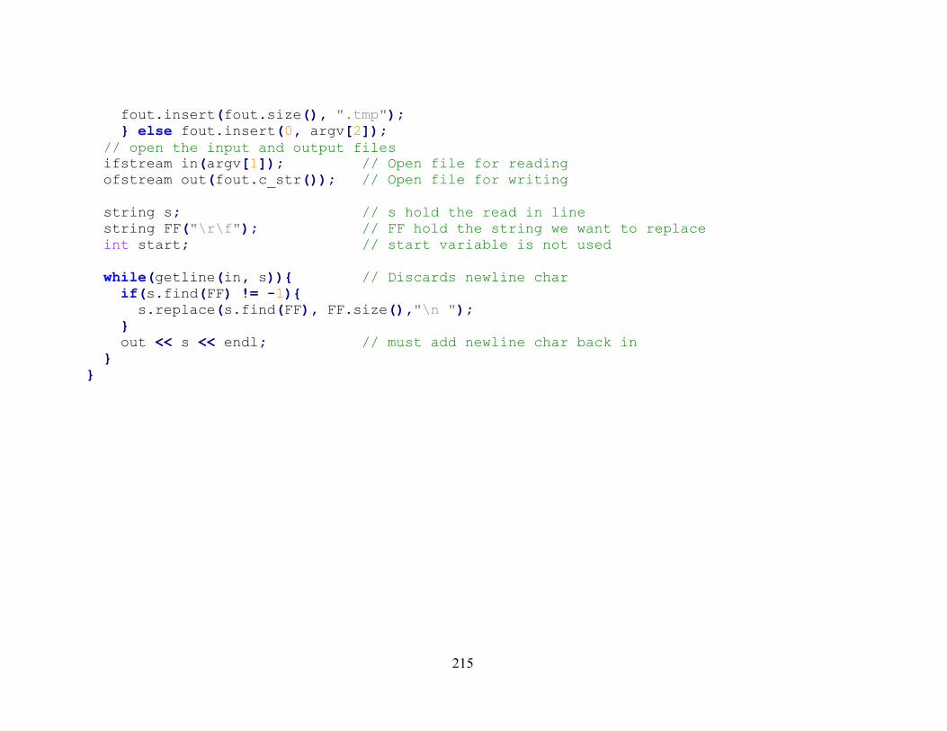
215
fout.insert(fout.size(), ".tmp"); } else fout.insert(0, argv[2]); // open the input and output files ifstream in(argv[1]); // Open file for reading ofstream out(fout.c_str()); // Open file for writing string s; // s hold the read in line string FF("\r\f"); // FF hold the string we want to replace int start; // start variable is not used while(getline(in, s)){ // Discards newline char if(s.find(FF) != -1){ s.replace(s.find(FF), FF.size(),"\n "); } out << s << endl; // must add newline char back in } }

216
:: ::===================================================================================== :: :: Filename: remove_headers.bat :: :: Description: This MSDOS batch files removes extraneous header information for :: the output data file created by PSS/E's plotting program. :: :: Precondition: The provided ASCII text data file must have all Form Feed ( FF ) :: characters removed, i.e., must have been processed by the :: "replace_FF_win_version.exe" program. :: :: Inputs: <Required> <column headings number> :: The column heading number control how many heading lines :: are used as the column headings. :: :: NOTE: This number is normally 0 or 1, where 0 indicates :: that no column heading is needed (i.e., just data :: without and column headings) and 1 indicates :: that a one line column heading is desired with :: the data. :: :: <Required> <ASCII text data input filename> :: The input data filename specifies the file with the :: ASCII text with the extra heading information. :: :: <Optional> <ASCII Text data output filename> :: This output data filename indicates that the process :: data file should be saved in the current directory with :: the given output filename. ::

217
:: If the output filename is omitted, then the processed :: data is sent to the standard output device, i.e., stdout. :: This is normally the command line terminal. :: :: Version: 1.0 :: Created: 6/10/2011 8:45:41 AM :: Revision: none :: Compiler: none :: :: Author: Jose E. Fadul (jef), :: Company: AFIT :: ::===================================================================================== :: :: :: The following command disables the auto-echoing of batch file commands. :: @echo off :: :: The following command enables extra batch file set command features, such as, :: mathematical calculations in conjunction with batch variable value assignments. :: setlocal enabledelayedexpansion :: :: The following two lines check for the required parameters. :: :: If the parameters are missing goto the usage label and provide some basic usage :: information.

218
:: :: If the parameters are present then continue. :: if [%1] == [] goto usage if [%2] == [] goto usage :: :: Set the column header counter variable to zero. :: SET /a counter=0 :: :: If the third command line variable is omitted, then send processed data to :: standard output device, i.e., stdout which is normally the command line terminal. :: if [%3] == [] goto stdout :: :: If the output data filename exist, then delete it without any warning. :: del /Q %3 2>NUL :: :: The following FOR loop extracts the desired number of column heading lines from :: the given input data file to the given output data file. :: FOR /F "skip=5 usebackq tokens=* delims=" %%i in (%2) do ( if "!counter!"=="%1" goto next1 echo %%i >> %3 SET /a counter+=1 )
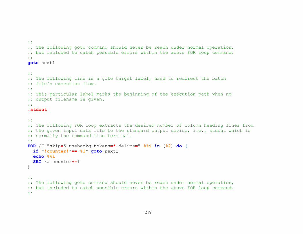
219
:: :: The following goto command should never be reach under normal operation, :: but included to catch possible errors within the above FOR loop command. :: goto next1 :: :: The following line is a goto target label, used to redirect the batch :: file's execution flow. :: :: This particular label marks the beginning of the execution path when no :: output filename is given. :: :stdout :: :: The following FOR loop extracts the desired number of column heading lines from :: the given input data file to the standard output device, i.e., stdout which is :: normally the command line terminal. :: FOR /F "skip=5 usebackq tokens=* delims=" %%i in (%2) do ( if "!counter!"=="%1" goto next2 echo %%i SET /a counter+=1 ) :: :: The following goto command should never be reach under normal operation, :: but included to catch possible errors within the above FOR loop command. ::

220
goto next2 :: :: The following line is a goto target label, used to redirect the batch :: file's execution flow. :: :: This particular label marks the beginning of the usage information provided :: to the user to help them use this batch file correctly. :: :usage echo. echo Usage: remove_headers.bat ^<column heading line number^> ^<input_filename^> [^<output_filename^>] echo. echo note: column heading line number is off-set by 5, i.e. for the sixth file line enter 1. echo. :: :: The following goto statement terminates this batch file's execution by :: going to the end of this file. :: goto exit :: :: This is legacy comment information created and referenced during development. :: rem example: remove_headers.bat 0 50_results_20100930_1135_v2.DAT 50_results_20100930_1135_v2.txt rem rem OR rem rem remove_headers.bat 1 50_results_20100930_1135_v2.DAT 50_results_20100930_1135_v2.txt rem rem The column heading line number specifies which line is the column heading line. rem This line number is off-set by 5, i.e. for the sixth file line enter a value of 1. rem A value of zero indicates that no column heading is desired in the output.

221
:: :: The following line is a goto target label, used to redirect the batch :: file's execution flow. :: :: This particular label marks the continuation of the execution path when an :: output filename is given. :: :next1 :: :: The following multi-piped findstr commands are used to extract the data values from :: the given input data file and appends them to the given output data file. :: :: The findstr command perform the following string processing actions: :: :: ( 1 ) findstr /v /i "pti identification IEEE Channel TIME" %2 :: This findstr command removes all the lines containing :: any one of the given words from the input data file. Hence, the lines without :: any of these given words is piped to the next findstr command. :: :: ( 2 ) findstr /R /V "^.$" :: This command removes all the lines that contain only one character. The lines :: with 2 or more characters, as well as, blank lines are piped to the next :: findstr command. :: :: ( 3 ) findstr /R /V "^$" :: This final findstr command removes all the blank lines from the input data. :: Hence only the data lines with 2 or more characters are appended to the given :: output data file. ::
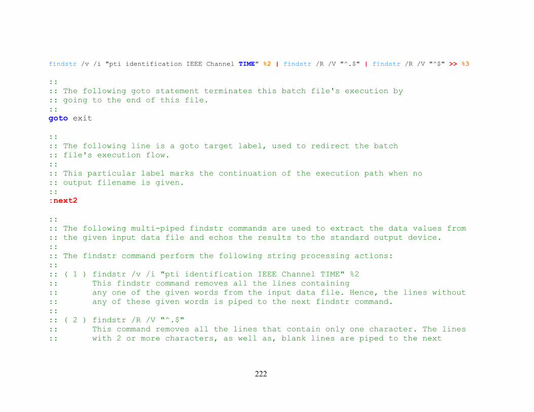
222
findstr /v /i "pti identification IEEE Channel TIME" %2 | findstr /R /V "^.$" | findstr /R /V "^$" >> %3 :: :: The following goto statement terminates this batch file's execution by :: going to the end of this file. :: goto exit :: :: The following line is a goto target label, used to redirect the batch :: file's execution flow. :: :: This particular label marks the continuation of the execution path when no :: output filename is given. :: :next2 :: :: The following multi-piped findstr commands are used to extract the data values from :: the given input data file and echos the results to the standard output device. :: :: The findstr command perform the following string processing actions: :: :: ( 1 ) findstr /v /i "pti identification IEEE Channel TIME" %2 :: This findstr command removes all the lines containing :: any one of the given words from the input data file. Hence, the lines without :: any of these given words is piped to the next findstr command. :: :: ( 2 ) findstr /R /V "^.$" :: This command removes all the lines that contain only one character. The lines :: with 2 or more characters, as well as, blank lines are piped to the next

223
:: findstr command. :: :: ( 3 ) findstr /R /V "^$" :: This final findstr command removes all the blank lines from the input data. :: Hence only the data lines with 2 or more characters are echoed to the :: standard output device, stdout which is normally the command line terminal. :: findstr /v /i "pti identification IEEE Channel TIME" %2 | findstr /R /V "^.$" | findstr /R /V "^$" :: :: The following line is a goto target label, used to redirect the batch :: file's execution flow. :: :: This particular label marks the end of this batch file and is used to end :: this batch file's execution. :: :exit

224
:: ::===================================================================================== :: :: Filename: R_cmd.bat :: :: Description: This MSDOS batch file executes an R script with a given data file. :: :: Inputs: <Required> data file :: The input data file is a two column ASCII text data file :: with the file column containing time data in seconds and :: the second column containing frequency data in :: per unit ( PU ) units. :: :: NOTE: The conversion formula from PU units to :: Hertz ( Hz ) units is: :: :: Hertz_Value = 60 * ( 1 + PU_value ) :: :: Version: 1.0 :: Created: 6/10/2011 8:45:18 AM :: Revision: none :: Compiler: none :: :: Author: Jose E. Fadul (jef), :: Company: AFIT :: ::===================================================================================== :: :: :: The following command disables the auto-echoing of batch file commands.

225
:: @echo off :: :: The following command uses the "R.exe" program to process the "plot_data_pdf.r" :: script. This script uses two input arguments, namely the current directory "%~dp0" :: and the name of the passed-in data filename "%1". :: :: The R.exe switches are used for: :: --vanilla means don't restore the R environment settings, :: don't read the user environment file, site environment file, :: or the Rprofile files and :: don't save the session :: :: -q Supress the startup message :: :: --slave Run as quietly as possible :: :: -f "file" use the given script file for R command inputs :: :: --args The rest of the command contains arguments for the R script file :: C:\R\R-2.11.1\bin\R --vanilla -q --slave -f "%~dp0/plot_data_pdf.r" --args "%~dp0" "%1"

226
## ##===================================================================================== ## ## Filename: plot_data_pdf.r ## ## Description: This R script file is used to plot the frequency data generated by ## PSS/E simulations. ## ## Inputs: <Required> path ## This is the path to the current working directory where ## The input data file is located and where the resulting ## PDF file will be stored. ## ## <Required> data filename ## This is the input data filename formatted in two columns ## of space delimited data, where the first column contains ## x-axis data values and the second column contains y-axis ## data values in Per Unit (PU) units. ## ## Version: 1.0 ## Created: 6/10/2011 4:44:36 PM ## Revision: none ## Compiler: none ## ## Author: Jose E. Fadul (jef), ## Company: AFIT ## ##===================================================================================== ## ##

227
## execute with "R --vanilla -q --slave -f <path>/plot_data_pdf.r --args <path> <filename>" ## ##################################################### # get working directory path and csv filename ##################################################### x <- commandArgs(TRUE); ##################################################### # Set working directory path ##################################################### setwd(x[1]); ##################################################### # Check for graphics package ##################################################### require(graphics); ##################################################### # Get data from Comma Separated Values (csv) file ##################################################### # d<-read.table(x[2],header=T,sep=",",quote="\""); ##################################################### # Get data from space delimited ASCII data file ##################################################### d<-read.table(x[2],header=T); n<-names(d)[2:length(d)]; j=1;
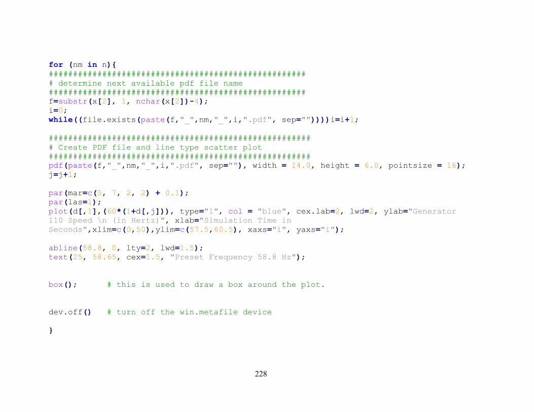
228
for (nm in n){ ##################################################### # determine next available pdf file name ##################################################### f=substr(x[2], 1, nchar(x[2])-4); i=0; while((file.exists(paste(f,"_",nm,"_",i,".pdf", sep=""))))i=i+1; ###################################################### # Create PDF file and line type scatter plot ###################################################### pdf(paste(f,"_",nm,"_",i,".pdf", sep=""), width = 14.0, height = 6.0, pointsize = 16); j=j+1; par(mar=c(5, 7, 2, 2) + 0.1); par(las=1); plot(d[,1],(60*(1+d[,j])), type="l", col = "blue", cex.lab=2, lwd=2, ylab="Generator 110 Speed \n (in Hertz)", xlab="Simulation Time in Seconds",xlim=c(0,50),ylim=c(57.5,60.5), xaxs="i", yaxs="i"); abline(58.8, 0, lty=2, lwd=1.5); text(25, 58.65, cex=1.5, "Preset Frequency 58.8 Hz"); box(); # this is used to draw a box around the plot. dev.off() # turn off the win.metafile device }

229
##################################################################### ## The following line used the Windows cmd.exe program to open the ## newly created PDF file. ##################################################################### cat(paste("start ",f,"_",nm,"_",i,".pdf\n", sep=""),file = "|cmd"); # End of File

230
Appendix H SPIN Model Checker ProMeLa Code
/* * ===================================================================================== * * Filename: minimal_SCADA_model_6.pml * * Description: This is a SPIN model representation of the Trust Management Toolkit. * This model specifically checks the detected fault response portion * of the Trust Management Toolkit by implementing the 3 major modules * in 4 basic steps; * * step 1. assign trust values <-- Assignment Module --> * step 2. fault_detected and send message <-- Detection Module --> * step 3. validate the detected fault <-- Decision Module --> * step 4. mitigate the validated fault <-- Decision Module --> * * Version: 1.0 * Created: 6/13/2011 12:21:24 PM * Revision: none * Compiler: spin and gcc * * Author: Jose E. Fadul (jef), * Company: AFIT * * ===================================================================================== */ // Number of Processes ( NP ) is 9 #define NP 9 // Number of Bus Nodes ( NN ) is 8

231
#define NN 8 // Fault Location #define FL 5 //////////////////////////////////////////////////////////////////////////////// // // system states: // no_errors is the initial state of the system // fault_validated is the system state when detected faults // are confirmed by 4 or more Agents. // fault_cleared is the system state after the validated fault is cleared. // //////////////////////////////////////////////////////////////////////////////// mtype = { no_errors, fault_validated, fault_cleared }; bit trust_value[ NP ] = 1; bit breaker[ NP ]; mtype system_state = no_errors; chan channel[ NP ] = [ 0 ] of { int }; active proctype SCADA() { int who, count; // step 1 assign trust values T0: atomic{ trust_value[ 4 ] = 0; trust_value[ 5 ] = 0; trust_value[ 6 ] = 0 }; do :: system_state == no_errors -> /* wait for error messages from nodes */ do :: channel[ 0 ]?who -> count = count + trust_value[ who ];

232
channel[ who ]!1; /* fault_detection acknowledgement message */ /* step 3 validate the detected fault */ system_state = (count > 3 -> fault_validated : no_errors) :: timeout -> break; od; :: system_state == fault_validated -> /* step 4 mitigate the validated fault */ who = FL; try_next_left: if :: who >= 1 && trust_value[ who ] -> channel[ who ]!1; :: who < 1 -> break; :: else -> who-- ; goto try_next_left; fi; who = FL + 1; try_next_right: if :: who <= 8 && trust_value[ who ] -> channel[ who ]!1; :: who > 8 -> break; :: else -> who++ ; goto try_next_right; fi; /* Confirm that the validated fault is isolated, i.e. cleared. */ count = 0; who = 1; do :: who <=8 -> count = count + breaker[ who ]; who++ :: else -> break; od; progress_0: system_state = ( count == 2 -> fault_cleared : fault_validated ); :: system_state == fault_cleared -> break od; assert( system_state == fault_cleared ); printf( "All messages received.\n" ); } active [ NN ] proctype Buss_Agents() {
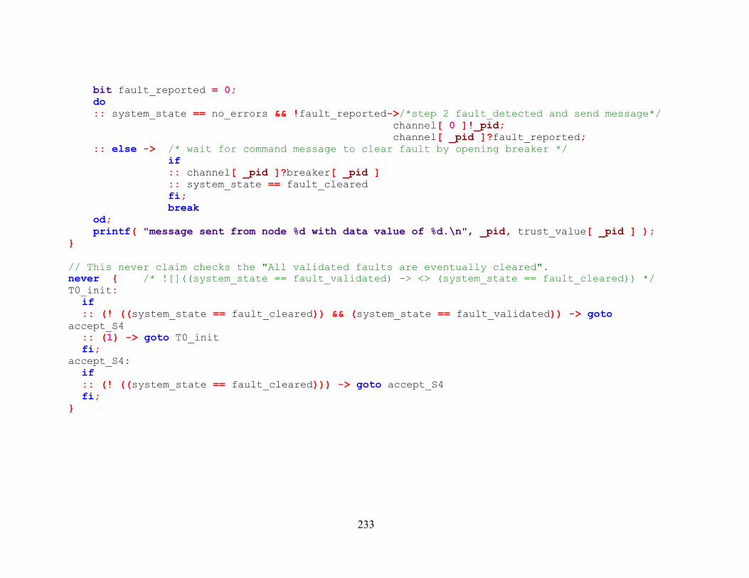
233
bit fault_reported = 0; do :: system_state == no_errors && !fault_reported->/*step 2 fault_detected and send message*/ channel[ 0 ]!_pid; channel[ _pid ]?fault_reported; :: else -> /* wait for command message to clear fault by opening breaker */ if :: channel[ _pid ]?breaker[ _pid ] :: system_state == fault_cleared fi; break od; printf( "message sent from node %d with data value of %d.\n", _pid, trust_value[ _pid ] ); } // This never claim checks the "All validated faults are eventually cleared". never { /*  -> <> (system_state == fault_cleared)) */ T0_init: if :: (! ((system_state == fault_cleared)) && (system_state == fault_validated)) -> goto accept_S4 :: (1) -> goto T0_init fi; accept_S4: if :: (! ((system_state == fault_cleared))) -> goto accept_S4 fi; }

234
// command: spin minimal_SCADA_model_6.pml // // warning: never claim not used in random simulation // timeout // message sent from node 3 with data value of 1. // message sent from node 7 with data value of 1. // message sent from node 4 with data value of 0. // message sent from node 8 with data value of 1. // All messages received. // message sent from node 2 with data value of 1. // message sent from node 6 with data value of 0. // message sent from node 1 with data value of 1. // message sent from node 5 with data value of 0. // 9 processes created // // command: spin -a minimal_SCADA_model_6.pml // cc -o pan pan.c // ./pan -a // // warning: for p.o. reduction to be valid the never claim must be stutter-invariant // (never claims generated from LTL formulae are stutter-invariant) // Depth= 201 States= 1e+06 Transitions= 5.1e+06 Memory= 66.563 t= 10.3 R= 1e+05 // Depth= 201 States= 2e+06 Transitions= 9.95e+06 Memory= 133.067 t= 20.2 R= 1e+05 // pan: resizing hashtable to -w21.. done // // (Spin Version 6.0.1 -- 16 December 2010) // + Partial Order Reduction // // Full statespace search for: // never claim + (never_0) // assertion violations + (if within scope of claim) // acceptance cycles + (fairness disabled) // invalid end states - (disabled by never claim)

235
// // State-vector 156 byte, depth reached 201, errors: 0 // 2045462 states, stored (2.34843e+06 visited) // 9365691 states, matched // 11714121 transitions (= visited+matched) // 0 atomic steps // hash conflicts: 8445624 (resolved) // // Stats on memory usage (in Megabytes): // 335.521 equivalent memory usage for states (stored*(State-vector + overhead)) // 156.873 actual memory usage for states (compression: 46.75%) // state-vector as stored = 64 byte + 16 byte overhead // 8.000 memory used for hash table (-w21) // 0.305 memory used for DFS stack (-m10000) // 164.993 total actual memory usage // // unreached in proctype SCADA // (0 of 44 states) // unreached in proctype Busses // (0 of 14 states) // unreached in claim never_0 // minimal_SCADA_model_5.pml:81, state 11, "-end-" // (1 of 11 states) // // pan: elapsed time 23.9 seconds // pan: rate 98108.786 states/second // // command: spin -a minimal_SCADA_model_6.pml // cc -DNP -o pan pan.c // ./pan -l // // Depth= 148 States= 1e+06 Transitions= 5.11e+06 Memory= 40.587 t= 9.69 R= 1e+05 // Depth= 201 States= 2e+06 Transitions= 1.08e+07 Memory= 80.137 t= 20.3 R= 1e+05 // pan: resizing hashtable to -w21.. done

236
// Depth= 201 States= 3e+06 Transitions= 1.75e+07 Memory= 148.098 t= 32.4 R= 9e+04 // Depth= 201 States= 4e+06 Transitions= 2.33e+07 Memory= 202.883 t= 42.4 R= 9e+04 // Depth= 201 States= 5e+06 Transitions= 2.98e+07 Memory= 260.403 t= 53.9 R= 9e+04 // pan: resizing hashtable to -w23.. done // // (Spin Version 6.0.1 -- 16 December 2010) // + Partial Order Reduction // // Full statespace search for: // never claim + (:np_:) // assertion violations + (if within scope of claim) // non-progress cycles + (fairness disabled) // invalid end states - (disabled by never claim) // // State-vector 156 byte, depth reached 201, errors: 0 // 3484843 states, stored (5.22719e+06 visited) // 26163073 states, matched // 31390265 transitions (= visited+matched) // 0 atomic steps // hash conflicts: 13388922 (resolved) // // Stats on memory usage (in Megabytes): // 571.626 equivalent memory usage for states (stored*(State-vector + overhead)) // 271.750 actual memory usage for states (compression: 47.54%) // state-vector as stored = 66 byte + 16 byte overhead // 32.000 memory used for hash table (-w23) // 0.305 memory used for DFS stack (-m10000) // 303.829 total actual memory usage // // unreached in proctype SCADA // (0 of 44 states) // unreached in proctype Busses // (0 of 14 states) // unreached in claim never_0

237
// minimal_SCADA_model_5.pml:74, state 5, "((!((system_state==fault_cleared))&&(system_state==fault_validated)))" // minimal_SCADA_model_5.pml:74, state 5, "(1)" // minimal_SCADA_model_5.pml:79, state 9, "(!((system_state==fault_cleared)))" // minimal_SCADA_model_5.pml:81, state 11, "-end-" // (3 of 11 states) // // pan: elapsed time 57.2 seconds // pan: rate 91430.83 states/second // //////////////////////////////////////////////////////////////////////////////// // // Removing the never claim process and running the following commands // yeilded the following output. // // Note: This output confirms that all modeled states are reachable. // //////////////////////////////////////////////////////////////////////////////// // command: spin -a minimal_SCADA_model_6.pml // cc -o pan pan.c // ./pan // // hint: this search is more efficient if pan.c is compiled -DSAFETY // Depth= 135 States= 1e+06 Transitions= 4.15e+06 Memory= 74.376 t= 6.88 R= 1e+05 // // (Spin Version 6.0.1 -- 16 December 2010) // + Partial Order Reduction // // Full statespace search for: // never claim - (none specified) // assertion violations + // acceptance cycles - (not selected) // invalid end states + //

238
// State-vector 152 byte, depth reached 135, errors: 0 // 1686666 states, stored // 5552000 states, matched // 7238666 transitions (= stored+matched) // 0 atomic steps // hash conflicts: 5290985 (resolved) // // Stats on memory usage (in Megabytes): // 270.233 equivalent memory usage for states (stored*(State-vector + overhead)) // 121.709 actual memory usage for states (compression: 45.04%) // state-vector as stored = 60 byte + 16 byte overhead // 2.000 memory used for hash table (-w19) // 0.305 memory used for DFS stack (-m10000) // 123.887 total actual memory usage // // unreached in proctype SCADA // (0 of 54 states) // unreached in proctype Busses // (0 of 14 states) // // pan: elapsed time 12.3 seconds // pan: rate 137339.47 states/second

239
Bibliography [1] U.S.-Canada Power System Outage Task Force. and United States. Dept. of
Energy., Final report on the August 14, 2003 blackout in the United States and Canada [electronic resource] : causes and recommendations / U.S.-Canada Power System Outage Task Force: U.S. Dept. of Energy, [Washington, D.C.] :, 2004.
[2] G. Bindewald, "Transforming the Grid to Revolutionize Electric Power in North America," presented at the Edison Electric Institute’s Fall 2003 Transmission, Distribution and Metering Conference, 2003.
[3] J. Ballman, "The Great Blackout of 2003 Aug. 14 Power Outage Largest in U.S. History," Disaster Recovery Journal, vol. 16, 2003.
[4] Electricity Consumers Resource Council (ELCON), "The Economic Impacts of the August 2003 Blackout," 2004.
[5] P. L. Anderson and I. K. Geckil, "Northeast Blackout Likely to Reduce US Earnings by $6.4 Billion," Anderson Economic Group (AEG), Working Paper 2003-2, 2003.
[6] L. Neergaard, "Emergency officials struggle to find those on life-support during power outages," 2009.
[7] Office of the President, "Presidential Decision Directives (PDD) 39: Counterterrorism Policy," 1995.
[8] Office of the President, "Presidential Decision Directives (PDD) 62: Protection Against Unconventional Threats to the Homeland and Americans Overseas," 1998.
[9] Office of the President, "Presidential Decision Directives (PDD) 63: Critical Infrastructure Protection," 1998.
[10] Office of the President, "The National Strategy for the Physical Protection of Critical Infrastructure and Key Assets," 2003.
[11] Office of the President, "Homeland Security Presidential Directive (HSPD) 7: Critical Infrastructure Identification, Prioritization, and Protection," 2003.
[12] M. Hathaway, "Cyberspace Policy Review: Assuring a Trusted and Resilient Information and Communications Infrastructure," 2009.
[13] J. Meserve, "Sources: Staged cyber attack reveals vulnerability in power grid ", Washington, D.C.: CNN, 2007.
[14] SANS NewsBites, "SANS Security Trade Conference," New Orleans, LA: SANS Institute, 2008.
[15] A. Greenberg, "Hackers Cut Cities' Power," Forbes.com, 2008. [16] Jpost staff and Associated Press (AP), "US weekly: Syrian radar destroyed before
strike," JPost.com, 2007. [17] J. Davis. (2007) Hackers Take Down the Most Wired Country in Europe. Wired
Magazine. Available: http://www.wired.com/print/politics/security/magazine/15-09/ff_estonia
[18] U.S. Engery Information Administration (EIA), "Annual Energy Outlook 2010 with Projections to 2035," U.S. Department of Energy (DOE) DOE/EIA-0383(2010), 2010.

240
[19] Y. Sverdlik, "Is the smart grid an intelligent move," Datacenter Dynamics FOCUS, vol. 3, pp. 21--22, February/March 2010.
[20] R. Lamb, "How a Microgrid Works," HowStuffWorks.com, 2009. [21] Office of the National Coordinator for Smart Grid Interoperability, "NIST
Framework and Roadmap for Smart Grid Interoperability Standards, Release 1.0," U.S. Department of Commerce and National Institute of Standards and Technology, NIST Special Publication 1108, 2010.
[22] Litos Strategic Communication, "WHAT A SMART GRID MEANS TO OUR NATION'S FUTURE.," U.S. Department of Energy Office of Electricity Delivery and Energy Reliability2009.
[23] L. Lamport, R. Shostak, and M. Pease, "The Byzantine Generals Problem," ACM Transactions on Programming Languages and Systems (TOPLAS), vol. 4, pp. 382-401, 1982.
[24] K. M. Hopkinson, K. P. Birman, R. Giovanini, D. V. Coury, X. Wang, and J. S. Thorp, "Distributed simulation in manufacturing: EPOCHS: integrated commercial off-the-shelf software for agent-based electric power and communication simulation," in WSC '03: Proceedings of the 35th conference on Winter simulation, 2003, pp. 1158-1166.
[25] G. M. Coates, K. M. Hopkinson, S. R. Graham, and S. H. Kurkowski, "Collaborative, Trust-Based Security Mechanisms for a Regional Utility Intranet," Power Systems, IEEE Transactions on, vol. 23, pp. 831-844, 2008.
[26] R. K. Ahuja, T. L. Magnanti, and J. B. Orlin, Network flows : theory, algorithms, and applications: Prentice Hall, Englewood Cliffs, N.J. :, 1993.
[27] J. Kleinberg and E. Tardos, Algorithm Design. Boston, MA, USA: Addison-Wesley Longman Publishing Co., Inc., 2005.
[28] IEEE, IEEE 100: The authoritative dictionary of IEEE standards terms, 7th ed.: IEEE Press, 2000.
[29] P. M. Anderson and B. K. LeReverend, "Industry experience with special protection schemes," Power Systems, IEEE Transactions on, vol. 11, pp. 1166-1179, 1996.
[30] J. E. Fadul, K. M. Hopkinson, T. R. Andel, J. T. Moore, and S. H. Kurkowski, "Simple Trust Protocol for Wired and Wireless SCADA networks," in 5th International Conference on Information Warfare and Security, Dayton, OH, 2010, pp. 89-97.
[31] Manitoba HVDC Research Centre Inc, "Power System Computer Aided Design," 1981.
[32] S. Mccanne, S. Floyd, and K. Fall, "ns2 (network simulator 2)," 1989. [33] D. Al-Arayed, "A Survey of Trust Management Systems," unpublished. [34] J. Huang and M. S. Fox, "An ontology of trust: formal semantics and transitivity,"
in ICEC '06: Proceedings of the 8th international conference on Electronic commerce, New York, NY, USA, 2006, pp. 259-270.
[35] T. Grandison and M. Sloman, "A Survey of Trust in Internet Applications," IEEE Communications Surveys and Tutorials, vol. 3, pp. 2-16, 2000-09 2000.
[36] R. Falcone and C. Castelfranchi, "Social trust: a cognitive approach," pp. 55-90, 2001.

241
[37] S. Ganeriwal, L. K. Balzano, and M. B. Srivastava, "Reputation-based framework for high integrity sensor networks," ACM Trans. Sen. Netw., vol. 4, pp. 1-37, 2008.
[38] S. Marsh and F. La, "Trust and Reliance in Multi-Agent Systems: A Preliminary Report," in In Proceedings of the 4th European Workshop on Modeling Autonomous Agents in a Multi-Agent World, 1992.
[39] M. Blaze, J. Feigenbaum, and J. Lacy, "Decentralized Trust Management," in Proceedings of the 1996 IEEE Symposium on Security and Privacy, 1996, pp. 164-173.
[40] P. R. Zimmermann, The Official PGP User's Guide. Cambridge, MA, USA: MIT Press, 1995.
[41] R. Housley, W. Polk, W. Ford, and D. Solo, "Internet X.509 Public Key Infrastructure Certificate and Certificate Revocation List (CRL) Profile," IETF, 2002.
[42] S. Buchegger and J.-Y. L. Boudec, "Performance analysis of the CONFIDANT protocol," in MobiHoc '02: Proceedings of the 3rd ACM international symposium on Mobile ad hoc networking & computing, New York, NY, USA, 2002, pp. 226-236.
[43] S. D. Kamvar, M. T. Schlosser, and H. Garcia-Molina, "The Eigentrust algorithm for reputation management in P2P networks," in WWW '03: Proceedings of the 12th international conference on World Wide Web, New York, NY, USA, 2003, pp. 640-651.
[44] V. M. Igure, S. A. Laughter, and R. D. Williams, "Security issues in SCADA networks," Computers & Security, vol. 25, pp. 498 - 506, 2006.
[45] X. R. Wang, K. M. Hopkinson, J. S. Thorp, R. Giovanini, K. Birman, and D. Coury, "Developing an Angent-based Backup Protection System for Transmission Networks," in First International Conference on Power Systems and Communication Systems Infrastructures for the Future, Beijing, China, 2002.
[46] R. Jain, The Art of Computer Systems Performance Analysis: Techniques for Experimental Design, Measurement, Simulation, and Modeling,. New York, NY, USA: Wiley-In-ter-sci-ence, 1991.
[47] D. Estrin, M. Handley, J. Heidemann, S. McCanne, Y. Xu, and H. Yu, "Network Visualization with Nam, the VINT Network Animator," Computer, vol. 33, pp. 63-68, 2000.
[48] J. E. Fadul, K. M. Hopkinson, T. R. Andel, J. T. Moore, and S. H. Kurkowski, "SCADA Trust Management System," in 2010 International Conference on Security and Management (SAM'10) (under The 2010 World Congress in Computer Science, Computer Engineering, and Applied Computing (WORLDCOMP'2010)), Las Vegas, Nevada USA, 2010, pp. 548 - 554.
[49] R. F. Dacey, "Congressional Testimony on Cybersecurity," U. S. Congress House Government Reform Committee Subcommittee on Technology, Information Policy, Intergovernmental Relations, and the Census 32Y3894059689, 2004.
[50] M. Brain, "How Power Grids Work," 2000. [51] H.R.6–110th Congress, Energy Independence and Security Act (EISA) of 2007:
GovTrack.us (database of federal legislation), 2007.

242
[52] R. F. Dacey, "Congressional Testimony on Critical Infrastructure Protection: Significant Challenges Need to be Addressed," U. S. Congress House of Representatives Government Reform Committee, Subcommittee on Government Efficiency, Financial Management and Intergovernmental Relations, Congressional Testimony GAO-02-961T, 2002.
[53] S. P. Marsh, "Formalizing Trust as a Computational Concept," Ph.D. Thesis, University of Stirling, 1994.
[54] L. R. Ford Jr. and D. R. Fulkerson, Flows in Networks. Princeton, N.J., U.S.A.: Princeton University Press, 1962.
[55] A. V. Goldberg, "HIgh-level Push-Relabel (HIPR) flow algorithm version 3.6," 2006.
[56] N. D. Curet, J. DeVinney, and M. E. Gaston, "An efficient network flow code for finding all minimum cost s-t cutsets," Computers & Operations Research, vol. 29, pp. 205 - 219, 2002.
[57] M. S. Bazaraa, J. J. Jarvis, and H. D. Sherali, Linear programming and network flows, 2nd ed.: John Wiley & Sons, Inc., 1990.
[58] N. Christofides, Graph Theory - An Algorithmic Approach. New York, NY: Academic Press, 1975.
[59] J. E. Fadul, K. M. Hopkinson, T. R. Andel, and J. T. Moore, "Trust Management and Security in the Future Communication-Based “Smart” Electric Power Grid," in 44 Hawaii International Conference on System Sciences (HICSS) (Electric Power Systems: reliability, Security, and Trust Track), Koloa, Kauai, Hawaii, January 4-7, 2011, pp. 1-10.
[60] S. Sutanto and R. Page Heller, "Utility communications architecture review," ISA Transactions, vol. 32, pp. 297-300, 1993.
[61] T. Kostic, O. Preiss, and C. Frei, "Understanding and using the IEC 61850: a case for meta-modelling," Computer Standards & Interfaces, vol. 27, pp. 679-695, 2005.
[62] B. Naduvathuparambil, M. C. Valenti, and A. Feliachi, "Communication Delays in Wide Area Measurement Systems," 2002, pp. 118 - 122.
[63] J. E. Dagle, "North American SynchroPhasor Initiative," 2008, pp. 165-165. [64] General Electric. PSLF Manual. 2003. Available:
http://www.gepower.com/dhtml/corporate/en_us/assets/software_solns/prod/pslf.jsp
[65] Shaw Power Technologies Inc., PSS/E 30 User's Manual. Schenectady, NY, USA, 2004.
[66] Manitoba HVDC Research Centre, PSCAD/EMTDC Manual Getting Started. Winnipeg, Manitoba, Canada, 1998.
[67] L. Breslau, D. Estrin, K. Fall, S. Floyd, J. Heidermann, A. Helmy, P. Huang, S. McCanne, K. Varadhan, Y. Xu, and H. Yu, "Advances in Network Simulation," IEEE Computer, vol. 33, pp. 59-67, May 2000.
[68] K. Hopkinson, X. Wang, R. Giovanini, J. Thorp, K. Birman, and D. Coury, "EPOCHS: A Platform for Agent-based Electric Power and Communication Simulation Built from Commercial Off-The-Shelf Components," IEEE Transactions on Power Systems, vol. 21, pp. 548-558, May 2006.

243
[69] E. W. Dijkstra, "A Note on Two Problems in Connection with Graphs," Numerische Mathematik, vol. 1, pp. 269-271, 1959.
[70] G. Heineman, G. Pollice, and S. Selkow, Algorithms in a Nutshell: O'Reilly Media, Inc., 2008.
[71] J. E. Fadul, K. M. Hopkinson, T. R. Andel, and J. T. Moore, "A Trust Management Toolkit for Smart Grid Protection Systems," IEEE Transactions on Smart Grid, p. Submitted for publication, 2011.
[72] J. M. Ortman and C. E. Guarneri, "United States Population Projections: 2000 to 2050," United States Census Bureau, 2009.
[73] A. Schmidt, "A Population Perspective of the United States," Population Resource Center, 2004.
[74] R Development Core Team, "R: A Language and Environment for Statistical Computing," Vienna, Austria, 2009.
[75] Office of the President, "The National Strategy For The Physical Protection of Critical Infrastructures and Key Assets," 2003.
[76] J. F. Borowski, K. M. Hopkinson, J. W. Humphries, and B. J. Borghetti, "Reputation-Based Trust for a Cooperative Agent-Based Backup Protection Scheme," IEEE Transactions on Smart Grid, p. to be published.
[77] "Transient stability test systems for direct stability methods," Power Systems, IEEE Transactions on, vol. 7, pp. 37-43, 1992.
[78] G. C. Sitts, "Radio Pierces the Great Blackout," Broadcast Engineering, 1965. [79] S. S. SHAPIRO and M. B. WILK, "An analysis of variance test for normality
(complete samples)," Biometrika, vol. 52, pp. 591-611, December 1, 1965. [80] J. E. Fadul, K. M. Hopkinson, T. R. Andel, and J. T. Moore, "Developing a Trust
Based Protocol for a Fault Tolerant Distributive Wireless Network," in Workshop on Future Directions in Cyber-physical Systems Security, Newark, NJ 07102, 2009.
[81] Cygwin Group, "Cygwin: a Unix-like Environment for Windows," 2004. [82] Siemens, "Power System Simulator for Engineering," 1976.

244
Vita
Captain Jose E. Fadul enlisted in the U.S. Naval reserves in 1985 and served as an
Electronic Technician (ET). He graduated with honors from Thomas Edison High School
in Queens, NY in 1986. He transferred from the Naval reserves to the Air Force active
duty in 1986. He served in the Air Force as a Ground Radio Communications Specialist
from 1986 until 2001. He graduated with honors from the Air Force Ground Radio
Technical School at Keesler Air Force Base, MS in 1987. He graduated with honors from
the Air Force Ground Radio Narrowband Technical School at Wright-Patterson Air Force
Base, OH in 1993. His enlisted deployments include Incirlik Air Base, Turkey and
Dhahran Air Base, Saudi Arabia. He earned his Bachelor of Science in Electrical
Engineering (B.S.E.E.) degree (summa cum laude) from the University of Central Florida
(UCF) in 2001. His first assignment after commissioning as an officer in 2001 was at the
Air Force Research Laboratory at Wright-Patterson Air Force Base, OH. His second
assignment was to the Air Force Institute of Technology (AFIT), Wright-Patterson Air
Force Base, OH, where he received his Masters of Science in Electrical Engineering
(M.S.E.E.) degree and was inducted into the Eta Kappa Nu electrical and computer
engineering honor society in 2006. His third Air Force assignment was to the Air Force
Operational Test and Evaluation Center (AFOTEC) headquarters at Kirtland Air Force
Base, NM. His fourth assignment in the Air Force was back to the Air Force Institute of
Technology, Wright-Patterson Air Force Base, OH, where he earned his Doctorate of
Philosophy in Electrical Engineering (Ph.D.E.E.) degree and was inducted into the Tau
Beta Pi engineering honor society.

REPORT DOCUMENTATION PAGE Form Approved OMB No. 074-0188
The public reporting burden for this collection of information is estimated to average 1 hour per response, including the time for reviewing instructions, searching existing data sources, gathering and maintaining the data needed, and completing and reviewing the collection of information. Send comments regarding this burden estimate or any other aspect of the collection of information, including suggestions for reducing this burden to Department of Defense, Washington Headquarters Services, Directorate for Information Operations and Reports (0704-0188), 1215 Jefferson Davis Highway, Suite 1204, Arlington, VA 22202-4302. Respondents should be aware that notwithstanding any other provision of law, no person shall be subject to an penalty for failing to comply with a collection of information if it does not display a currently valid OMB control number. PLEASE DO NOT RETURN YOUR FORM TO THE ABOVE ADDRESS. 1. REPORT DATE (DD-MM-YYYY)
15-09-2011 2. REPORT TYPE
Doctoral Dissertation 3. DATES COVERED (From – To)
Sept 2008 – Sept 2011 4. TITLE AND SUBTITLE Using Reputation Based Trust to Overcome Malfunctions and Malicious Failures in Electric Power Protection Systems
5a. CONTRACT NUMBER
5b. GRANT NUMBER 5c. PROGRAM ELEMENT NUMBER
6. AUTHOR(S) Fadul, Jose E., Captain, USAF
5d. PROJECT NUMBER 11G292P 5e. TASK NUMBER
5f. WORK UNIT NUMBER
7. PERFORMING ORGANIZATION NAMES(S) AND ADDRESS(S) Air Force Institute of Technology Graduate School of Engineering and Management (AFIT/EN) 2950 Hobson Way, Building 640 WPAFB OH 45433-8865
8. PERFORMING ORGANIZATION REPORT NUMBER AFIT/DEE/ENG/11-08
9. SPONSORING/MONITORING AGENCY NAME(S) AND ADDRESS(ES) Air Force Office of Scientific Research, Mathematics, Information and Life Sciences Directorate Attn : Dr. Robert J. Bonneau 875 N Randolph St, Ste 325, Rm 3112, Arlington, VA 22203 (703) 696-9545 (DSN: 426-9545) Email: [email protected]
10. SPONSOR/MONITOR’S ACRONYM(S) AFOSR/NL 11. SPONSOR/MONITOR’S REPORT NUMBER(S)
12. DISTRIBUTION/AVAILABILITY STATEMENT DISTRIBUTION STATEMENT A: APPROVED FOR PUBLIC RELEASE; DISTRIBUTION UNLIMITED.
13. SUPPLEMENTARY NOTES This material is declared a work of the U.S. Government and is not subject to copyright protection in the United States. 14. ABSTRACT This dissertation advocates the use of reputation-based trust in conjunction with a trust management framework based on network flow techniques to form a trust management toolkit (TMT) for the defense of future Smart Grid enabled electric power grid from both malicious and non-malicious malfunctions. Increases in energy demand have prompted the implementation of Smart Grid technologies within the power grid. Smart Grid technologies enable Internet based communication capabilities within the power grid, but also increase the grid’s vulnerability to cyber attacks. The benefits of TMT augmented electric power protection systems include: improved response times, added resilience to malicious and non-malicious malfunctions, and increased reliability due to the successful mitigation of detected faults. In one simulated test case, there was a 99% improvement in fault mitigation response time. Additional simulations demonstrated the TMT’s ability to determine which nodes were compromised and to work around the faulty devices when responding to transient instabilities. This added resilience prevents outages and minimizes equipment damage from network based attacks, which also improves system’s reliability. The benefits of the TMT have been demonstrated using computer simulations of dynamic power systems in the context of backup protection systems and special protection systems. 15. SUBJECT TERMS SCADA, Trust Management System, Reputation-Base Trust, Cyber Security, Smart Grid, Power Grid
16. SECURITY CLASSIFICATION OF:
17. LIMITATION OF ABSTRACT
UU
18. NUMBER OF PAGES
268
19a. NAME OF RESPONSIBLE PERSON Kenneth M. Hopkinson, Civ, USAF (ENG)
a. REPORT
U b. ABSTRACT
U c. THIS PAGE
U 19b. TELEPHONE NUMBER (Include area code) (937) 255-6565, ext 4579 ([email protected])
Standard Form 298 (Rev. 8-98) Prescribed by ANSI Std. Z39-18


