Download - Age structure and Household Consumption in Brazil - ANPEC · 1 Age structure and Household Consumption in Brazil Flaviane Souza Santiago1, Mônica Viegas Andrade2, Edson Paulo Domingues3

1

Age structure and Household Consumption in Brazil

Flaviane Souza Santiago1, Mônica Viegas Andrade2, Edson Paulo Domingues3 and Geoffrey J.D. Hewings4

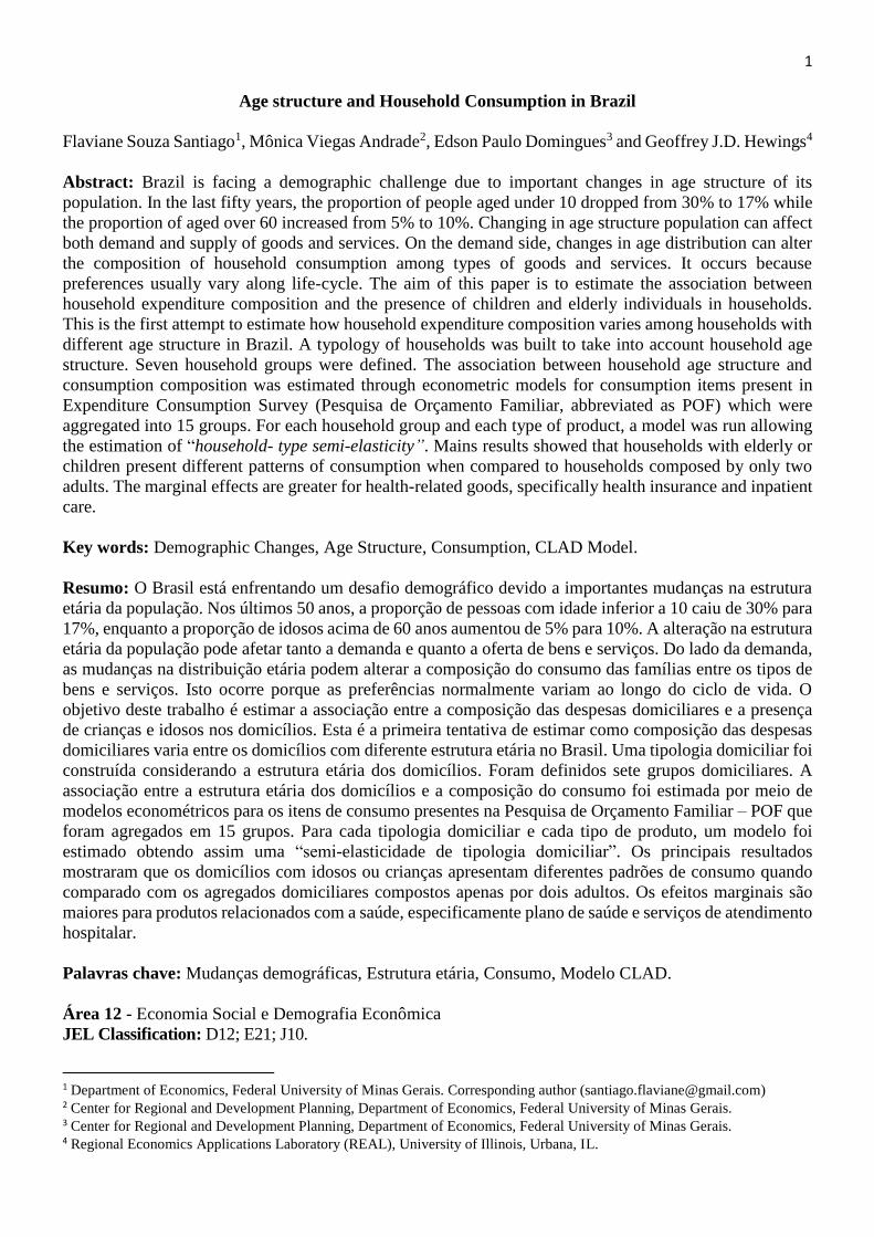
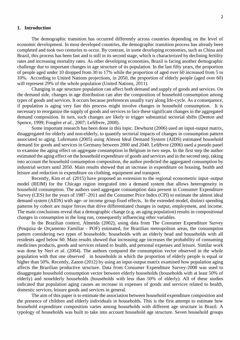
Abstract: Brazil is facing a demographic challenge due to important changes in age structure of its

population. In the last fifty years, the proportion of people aged under 10 dropped from 30% to 17% while

the proportion of aged over 60 increased from 5% to 10%. Changing in age structure population can affect

both demand and supply of goods and services. On the demand side, changes in age distribution can alter

the composition of household consumption among types of goods and services. It occurs because

preferences usually vary along life-cycle. The aim of this paper is to estimate the association between

household expenditure composition and the presence of children and elderly individuals in households.

This is the first attempt to estimate how household expenditure composition varies among households with

different age structure in Brazil. A typology of households was built to take into account household age

structure. Seven household groups were defined. The association between household age structure and

consumption composition was estimated through econometric models for consumption items present in

Expenditure Consumption Survey (Pesquisa de Orçamento Familiar, abbreviated as POF) which were

aggregated into 15 groups. For each household group and each type of product, a model was run allowing

the estimation of “household- type semi-elasticity”. Mains results showed that households with elderly or

children present different patterns of consumption when compared to households composed by only two

adults. The marginal effects are greater for health-related goods, specifically health insurance and inpatient

care.

Key words: Demographic Changes, Age Structure, Consumption, CLAD Model.

Resumo: O Brasil está enfrentando um desafio demográfico devido a importantes mudanças na estrutura

etária da população. Nos últimos 50 anos, a proporção de pessoas com idade inferior a 10 caiu de 30% para

17%, enquanto a proporção de idosos acima de 60 anos aumentou de 5% para 10%. A alteração na estrutura

etária da população pode afetar tanto a demanda e quanto a oferta de bens e serviços. Do lado da demanda,

as mudanças na distribuição etária podem alterar a composição do consumo das famílias entre os tipos de

bens e serviços. Isto ocorre porque as preferências normalmente variam ao longo do ciclo de vida. O

objetivo deste trabalho é estimar a associação entre a composição das despesas domiciliares e a presença

de crianças e idosos nos domicílios. Esta é a primeira tentativa de estimar como composição das despesas

domiciliares varia entre os domicílios com diferente estrutura etária no Brasil. Uma tipologia domiciliar foi

construída considerando a estrutura etária dos domicílios. Foram definidos sete grupos domiciliares. A

associação entre a estrutura etária dos domicílios e a composição do consumo foi estimada por meio de

modelos econométricos para os itens de consumo presentes na Pesquisa de Orçamento Familiar – POF que

foram agregados em 15 grupos. Para cada tipologia domiciliar e cada tipo de produto, um modelo foi

estimado obtendo assim uma “semi-elasticidade de tipologia domiciliar”. Os principais resultados

mostraram que os domicílios com idosos ou crianças apresentam diferentes padrões de consumo quando

comparado com os agregados domiciliares compostos apenas por dois adultos. Os efeitos marginais são

maiores para produtos relacionados com a saúde, especificamente plano de saúde e serviços de atendimento

hospitalar.

Palavras chave: Mudanças demográficas, Estrutura etária, Consumo, Modelo CLAD.

Área 12 - Economia Social e Demografia Econômica

JEL Classification: D12; E21; J10.

1 Department of Economics, Federal University of Minas Gerais. Corresponding author ([email protected]) 2 Center for Regional and Development Planning, Department of Economics, Federal University of Minas Gerais. 3 Center for Regional and Development Planning, Department of Economics, Federal University of Minas Gerais. 4 Regional Economics Applications Laboratory (REAL), University of Illinois, Urbana, IL.

2

1. Introduction

The demographic transition has occurred differently across countries depending on the level of

economic development. In most developed countries, the demographic transition process has already been

completed and took two centuries to occur. By contrast, in some developing economies, such as China and

Brazil, this process has been fast and is still in its second stage, which is characterized by declining fertility

rates and increasing mortality rates. As other developing economies, Brazil is facing another demographic

challenge due to important changes in age structure of its population. In the last fifty years, the proportion

of people aged under 10 dropped from 30 to 17% while the proportion of aged over 60 increased from 5 to

10%. According to United Nations projections, in 2050, the proportion of elderly people (aged over 60)

will represent 29% of the whole population (United Nations, 2011).

Changing in age structure population can affect both demand and supply of goods and services. On

the demand side, changes in age distribution can alter the composition of household consumption among

types of goods and services. It occurs because preferences usually vary along life-cycle. As a consequence,

if population is aging very fast this process might involve changes in household consumption. It is

necessary to reorganize the supply of goods and services to face these significant changes in the aggregated

demand composition. In turn, such changes are likely to trigger substantial sectorial shifts (Denton and

Spence, 1999; Fougère et al., 2007; Lefèbvre, 2008).

Some important research has been done in this topic. Dewhurst (2006) used an input-output matrix,

disaggregated for elderly and non-elderly, to quantify sectorial impacts of changes in consumption pattern

associated to aging. Luhrmann (2005) using Almost Ideal Demand System (AIDS) estimated household

demand for goods and services in Germany between 2000 and 2040. Lefèbvre (2006) used a pseudo panel

to examine the aging effect on aggregate consumption in Belgium in two steps. In the first step the author

estimated the aging effect on the household expenditure of goods and services and in the second step, taking

into account the household consumption composition, the author predicted the aggregated consumption by

industrial sectors until 2050. Main results showed that an increase in expenditure on housing, health and

leisure and reduction in expenditure on clothing, equipment and transport.

Recently, Kim et al. (2015) have proposed an extension to the regional econometric input–output

model (REIM) for the Chicago region integrated into a demand system that allows heterogeneity in

household consumption. The authors used aggregate consumption data present in Consumer Expenditure

Survey (CES) for the years of 1987–2011 and the Consumer Price Index (CPI) to estimate the almost ideal

demand system (AIDS) with age- or income group fixed effects. In the extended model, distinct spending

patterns by cohort are major forces that drive differentiated changes in output, employment, and income.

The main conclusions reveal that a demographic change (e.g. an aging population) results in compositional

changes in consumption in the long run, consequently influencing other variables.

In the Brazilian context, Almeida (2002), using data from The Consumer Expenditure Survey

(Pesquisa de Orçamento Familiar - POF) estimated, for Brazilian metropolitan areas, the consumption

pattern considering two types of households: households with an elderly head and households with all

residents aged below 60. Main results showed that increasing age increases the probability of consuming

medicines products, goods and services related to health, and personal expenses and leisure. Similar work

was done by Neri et al. (2004). The authors compared the consumption vector observed in the whole

population with that one observed in households in which the proportion of elderly people is equal or

higher than 50%. Recently, Zanon (2012) by using an input-output matrix examined how population aging

affects the Brazilian productive structure. Data from Consumer Expenditure Survey-2008 was used to

disaggregate household consumption vector between elderly households (households with at least 50% of

elderly) and nonelderly households (households with less than 50% of elderly). All of these studies

indicated that population aging causes an increase in expenses of goods and services related to health,

domestic services, leisure goods and services in general.

The aim of this paper is to estimate the association between household expenditure composition and

the presence of children and elderly individuals in households. This is the first attempt to estimate how

household expenditure composition varies among households with different age structure in Brazil. A

typology of households was built to take into account household age structure. Seven household groups

3

were defined. The association between household age structure and consumption composition was

estimated through econometric models. For each household group and each type of product a model was

run allowing the estimation of household- type semi-elasticity. All consumption items present in

Expenditure Consumption Survey were aggregated into 15 groups. In fact, 13 semi-elasticity’s coefficients

were estimated for each type of household. Finally, a consumption vector was also estimated for each

household group making it possible to compare the consumption pattern among households with different

age structure.

2. Data

This paper uses Consumer Expenditure Survey data set for the years of 2002-2003. This survey is

carried out by the Brazilian Institute of Geography and Statistics (Instituto Brasileiro de Geografia e

Estatística – IBGE, 2004) every five years. The main aim of this survey is to estimate household

consumption expenditure in order to subsidize the build of the National Consumer Price Index (INPC).

The 2002/2003 survey contains information about the population living in urban and rural areas in

Brazil. Its sample is representative for the 27 federal units, nine metropolitan areas, as well as for the whole

country. The sample size included 182,333 individuals living in 48,470 households. Data collection is

conducted through six questionnaires, five of them are organized according to type of expenditure: 1)

household and residents characteristics; 2) collective expenditure in durable household goods 3) collective

expenditure in food and cleaning, 4) individual expenditure; 5) individual earnings and wages. The last

questionnaire investigates living conditions perception (IBGE, 2004).

In this paper, we use all collective and individual expenditure items calculated and annualized by

IBGE. The expenditure of goods and services were mapped into 15 categories of goods and services: food,

textiles and clothing, fuel and transportation, medicines, health insurance, inpatient care , durables goods,

other goods, energy, private education, financial services and insurance, services, services provided to

families, food consumed out of the household and housing. Services provided to families include mainly

caregivers to elderly and children. All expenditures are calculated and annualized by IBGE.

3. Household Typology

In order to analyze aging effect on expenditure composition it is necessary to classify households

according to the presence of elderly residents and children. The classification of households is done taking

into account the number of adults (residents aged from 15 to 59 years stratified into two age groups), elderly

persons (residents aged over than 59 stratified into three age groups) and children (residents aged from 0 to

14 years stratified into three age groups) in the household. The disaggregation of elderly individuals and

children by age is important to allow the use demographic projections, even though their use is out of the

scope of this paper.

Seven types of households were defined: households with only two adults; households with two

adults and one child (0-4 years old, 5-9 years old, 10-14 years old); households with two adults aged from

15 to 49 and one adult aged from 50 to 59; households with two adults aged from 15 to 49 years and one

elderly aged from 60 to 69 and finally two adults aged from 15 to 49 years and one elderly over 70´s.

Households including only two adults (15-49) were considered as the reference category for the comparison

of expenditure composition. In order to allow the identification of aging effect, households with elderly and

children living together were excluded from the sample. The seven groups of households defined in our

typology represents 20% of the total sample (48.470 households) surveyed by POF in 2002-2003, that is,

9.516 households. Table 1 reports the distribution of households according to each group. The largest group

corresponds to households with only two adults (3.221 observations).

4

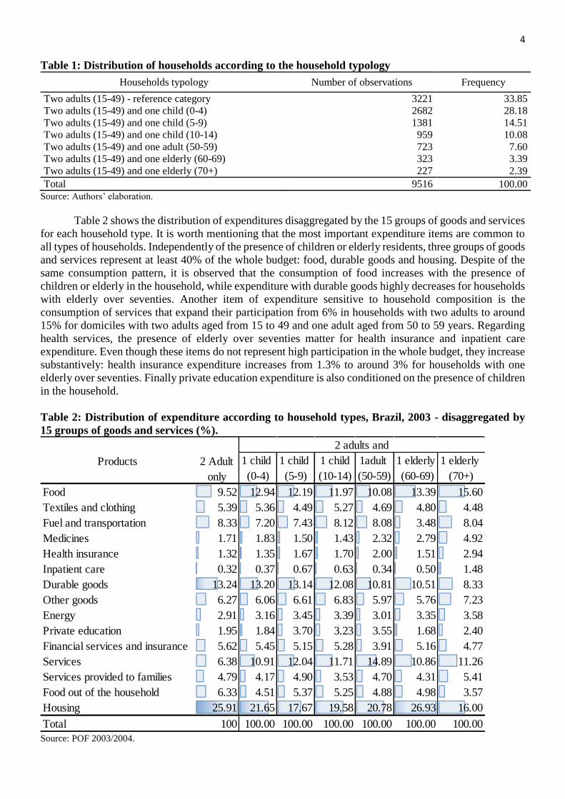
Table 1: Distribution of households according to the household typology

Households typology Number of observations Frequency

Two adults (15-49) - reference category 3221 33.85

Two adults (15-49) and one child (0-4) 2682 28.18



Two adults (15-49) and one adult (50-59) 723 7.60

Two adults (15-49) and one elderly (60-69) 323 3.39

Two adults (15-49) and one elderly (70+) 227 2.39

Total 9516 100.00

Source: Authors’ elaboration.

Table 2 shows the distribution of expenditures disaggregated by the 15 groups of goods and services

for each household type. It is worth mentioning that the most important expenditure items are common to

all types of households. Independently of the presence of children or elderly residents, three groups of goods

and services represent at least 40% of the whole budget: food, durable goods and housing. Despite of the

same consumption pattern, it is observed that the consumption of food increases with the presence of

children or elderly in the household, while expenditure with durable goods highly decreases for households

with elderly over seventies. Another item of expenditure sensitive to household composition is the

consumption of services that expand their participation from 6% in households with two adults to around

15% for domiciles with two adults aged from 15 to 49 and one adult aged from 50 to 59 years. Regarding

health services, the presence of elderly over seventies matter for health insurance and inpatient care

expenditure. Even though these items do not represent high participation in the whole budget, they increase

substantively: health insurance expenditure increases from 1.3% to around 3% for households with one

elderly over seventies. Finally private education expenditure is also conditioned on the presence of children

in the household.

Table 2: Distribution of expenditure according to household types, Brazil, 2003 - disaggregated by

15 groups of goods and services (%).

Source: POF 2003/2004.

1 child 1 child 1 child 1adult 1 elderly 1 elderly

(0-4) (5-9) (10-14) (50-59) (60-69) (70+)

Food 9.52 12.94 12.19 11.97 10.08 13.39 15.60

Textiles and clothing 5.39 5.36 4.49 5.27 4.69 4.80 4.48

Fuel and transportation 8.33 7.20 7.43 8.12 8.08 3.48 8.04

Medicines 1.71 1.83 1.50 1.43 2.32 2.79 4.92

Health insurance 1.32 1.35 1.67 1.70 2.00 1.51 2.94

Inpatient care 0.32 0.37 0.67 0.63 0.34 0.50 1.48

Durable goods 13.24 13.20 13.14 12.08 10.81 10.51 8.33

Other goods 6.27 6.06 6.61 6.83 5.97 5.76 7.23

Energy 2.91 3.16 3.45 3.39 3.01 3.35 3.58

Private education 1.95 1.84 3.70 3.23 3.55 1.68 2.40

Financial services and insurance 5.62 5.45 5.15 5.28 3.91 5.16 4.77

Services 6.38 10.91 12.04 11.71 14.89 10.86 11.26

Services provided to families 4.79 4.17 4.90 3.53 4.70 4.31 5.41

Food out of the household 6.33 4.51 5.37 5.25 4.88 4.98 3.57

Housing 25.91 21.65 17.67 19.58 20.78 26.93 16.00

Total 100 100.00 100.00 100.00 100.00 100.00 100.00

Products

2 adults and

2 Adult

only

5

3. Methodology

The aim of this paper is to analyze the effects of household composition, especially the presence of

elderly and child, will be explored in terms of the allocation of household expenditure on consumer goods.

Specifically, the effects of presence of elderly and children are measured through the estimation of demand

semi-elasticities of household composition.

One difficulty of estimating semi-elasticities on household expenditure regards data distribution.

Usually, there is a large portion of zeros, especially when household expenditure is disaggregated by

various products. The presence of high number of zeros occurs due to a significant fraction of households

present no any expenditure on various products. The tables 1 and 2 in the Appendix B reports the

expenditure distributions for all product groups taking into account the household typology. One possible

method of estimation is the Tobit Model which provides consistent estimates by maximum likelihood. The

censored regression analysis usually applies when the dependent variable is censored. Regarding

expenditure distributions, observations assume only non-negative values, which means, that data

distribution is left-censored at zero. In this cases, zero values are obtained as a result of the choice of optimal

consumption vector.

In a censored distribution, only values above the censoring point (in this case, expenditure = 0) are

relevant for the estimation of the dependent variable, which means a non-negative expenditure constraint

on the estimation of the expenses5. Typically, the Tobit model expresses the observed response ( y ) in

terms of an underlying latent variable. The general formulation of the Tobit model can be represented by

the following relation (Tobin, 1958):

uxy '* (1)

where *y is an unobserved latent variable, x is a 1k vector of control variables, is a 1k vector of

parameters to be estimated, and u is the random error term. The errors are assumed i.i.d., and in this case:

),0(~| 2Nxu (2)

In other words, the error term u has a constant 2 . This implies that the latent variable* 2~ ( , )y N x follows a normal homoscedastic distribution.

As the latent variable *y , is not observed in all its domain, it is defined a new random variable y ,

transformed from the original 𝑦∗, which represents the response observed only for values greater than zero

and which are censored for values equal to zero. In this case, it follows that:

),0max( *yy (3)

This implies that y equals *y when 0* y and y equals zero when 0* y . Formally, there is:

𝑦 = {𝑦∗ 𝑤ℎ𝑒𝑛 𝑦∗ > 00 𝑤ℎ𝑒𝑛 𝑦∗ ≤ 0

(4)

For a problem solving corner, | xE y has zero as the lower limit. Thus:

| max(0, )E y x x (5)

5 The usual least squares estimator fails in this case, being biased even in large samples where: a) the zeros in the data are kept

and treated like any other observation, or b) all zero observations are removed. Thus, the estimators for the coefficients would

be inconsistent (Wooldridge, 2000; Cameron and Trivedi, 2005; Cameron and Trivedi, 2009).

6

The conditional expectation of y is always non-negative. By the fact that *y is normally

distributed, y has a continuous distribution over strictly positive values. Particularly, the density of y

given x is the same as the density of y given x for positive values.

The Tobit model is based on homoscedastic variance of the error term u . If 2,0~ Nu – normal

and homoscedastic – then the ̂ estimator is consistent and efficient. Otherwise, it is inconsistent. Pagan

and Vella (1989) describe the conditional moment test that can be implemented after the Tobit model

estimation. If one of the null hypothesis of normality or homoscedasticity of errors is discarded, one option

is to use the Censored Least Absolute Deviations (CLAD) estimator (Powell, 1984; Wooldridge, 2000;

Cameron and Trivedi, 2005), which is consistent since the median | 0i iu Z .

3.1 Censored Least Absolute Deviations Estimator (CLAD) 6

The CLAD estimator is a generalization of the semiparametric estimator Least Absolute Deviations

(LAD) proposed by Powell (1984) as an alternative to the Tobit model when data distribution is

heteroscedastic. Unlike the standard censored regression estimator, Tobit, or other approaches by maximum

likelihood, the CLAD estimator is robust to heteroscedasticity being consistent and asymptotically normal

for a wide class of error distributions. The properties of the LAD estimator are presented in Koenker and

Basset (1978).

Starting from equation (1) and considering that the median of u given x equals zero:

0|* xuMeduxy (6)

Equation (6) implies that xxyMed | ; in this case the median of *y is linear in x . By the fact

that ),0max( *yy is a non-decreasing function, it follows that:

xxyMedxyMed ,0max|,0max| * (7)

As shown in equation (7), xyMed | does not depend on the distribution of u given x . xyE | and 0,| yxyE depend. In addition, the average and median functions have different forms. The

conditional median of y is zero for 0x and linear in x for 0x . In contrast, the conditional

expectation xyE | is never equal to zero and it is a nonlinear function of x . Note that equation (7) has the

equation (6) as its only hypothesis; no other hypothesis about the errors distribution is necessary. Thus, by

(7), the CLAD estimator ̂ can be estimated by the following minimization problem:

|,0max|min1

N

i

i xy

(8)

For the linear model, the CLAD method provides estimates of regression coefficients by minimizing

the sum of absolute residuals. It is a generalization of the sample median to the context of regression as

well as OLS is a generalization of the sample mean to the linear model. If the dependent variable *y is

observed, then the median is the regression function 'x under the condition that the errors have a median

equals zero. Thus, the estimated CLAD can be used to estimate the unknown coefficients (Wilhelm, 2008).

Powell shows that the consistency of this estimator does not depend on any other assumption about

the error distribution. Thus, u is robust to heteroscedasticity, consistent, and asymptotically normal for a

wide class of error distributions, since it only considers the median equals zero (see Deaton, 1997, Powell,

6 To this methodology, it was used as reference: Wilhelm, 2008; Wooldridge, 2000 and Powell (1984).

7

1984 and Buchinsky, 1994). The CLAD estimation procedure is operational by an algorithm proposed by

Buchinsky (1994) 7.

As a limitation of the model, the estimator requires that at least 50% of the observations are

uncensored. However, in some cases, depending on the context analyzed, another quantile than the median

can be used in estimate and the parameters are obtained from a censored quantile regression model (for

further details see Wooldridge, 2000; Buchinsky, 1994).

3.2 Model Specification

In this paper, an econometric model CLAD is run to estimate the semi-elasticities of types of

households. y. Additionally, a bootstrap procedure is estimated to obtain consistent estimations of standard

errors. The data source is 2002-2003 POF. One model for each product (except food and housing) and each

household type is estimated in order to obtain semi-elasticities of household composition. Six different

specifications for each product (13) are estimated. For all models the household reference category are

households with only two adults living. Semi-elasticities on food and housing expenditures are not

estimated because these types of expenditure are common to all individuals living in the household,

therefore it is not adequate to assume that elderly or children living in the domicile can cause variations in

the budget share of these consumption items.

In all household typologies only 25% of total households present positive expenditures on health

insurance and education (See Appendix A). Specifically for inpatient care, only 10% of households spend

with this product. As noted earlier, a limitation of the CLAD model lies in the fact that the estimator requires

that at least 50% of the observations are uncensored. In that manner, it is not possible to estimate median

semi-elaticities for these three products (education, hospital care, health insurance). In order to find a

solution, these products´ estimation were done using other quantiles. In these cases, Least Absolute

Deviations (LAD) model was used. For each type of household (k) 13 models were estimated corresponding

to different products (i). To accomplish this task 78 models were estimated, 13 products and 6 types of

household.

Table 3 describes dependent and independent variables included in the estimation. Independent

variables regards socioeconomic and demographic characteristics of households. The dependent variables

are the annual expenditure per product for each household typology. Households were classified in seven

categories according to the number of adults, elderly and children: households with two adults, two adults

and one child aged 0-4, two adults and a child of 5-9 years, two adults and one child 10-14, two adults and

one adult aged 50-59, two adults and an elderly 60-69, two adults and an elderly 70 years or more. The total

sample was split into k groups according to household typology. Each subsample was composed by

households with only two adults and households for each type defined in the household typology. In order

to identify each type of household a dummy variable was built corresponding to zero if the household is

composed by two adults (reference category) and 0 otherwise.

These dummy variables aim to capture marginal effects on consumption of goods and services

resulting from the presence of children and elderly in the domiciles.

Control variables concerns socioeconomic status, head of household characteristics and local of

residence. The annual total expenditure per capita is used as independent variable instead of the total annual

income. Annual total expenditure is a proxy for household permanent income, being therefore, more

adequate to estimate marginal effects regarding household composition. Usually household expenditure

fluctuates less than income because individuals can use savings or credit to finance their consumption.

Besides, it is less subject to measurement errors in the Consumer Expenditure Survey because individuals

have to register all expenditures in a booklet provided by the interviewer while income information is self-

reported. Schooling of household head is also included in the model as proxy variable to socioeconomic

status. It also allows to control for information effect. Individuals can choose to consume differently

conditioned on their information. It is particularly important for healthcare services and goods. The local

7 For further details, see Buchinsky (1994).

8

of residence is included because there may be regional differences in the cost of living. A categorical

variable was built considering 5 great regions in Brazil: Southeast, Northeast, North, South and Midwest.

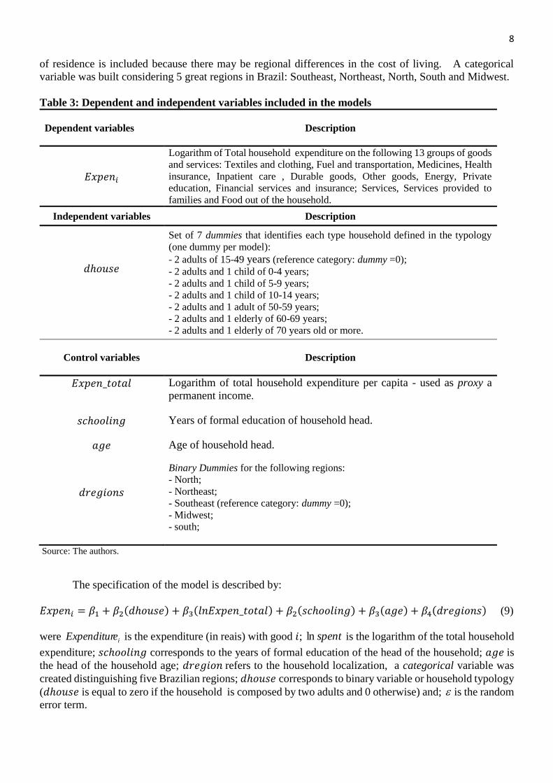
Table 3: Dependent and independent variables included in the models

Dependent variables

Description

𝐸𝑥𝑝𝑒𝑛𝑖

Logarithm of Total household expenditure on the following 13 groups of goods

and services: Textiles and clothing, Fuel and transportation, Medicines, Health

insurance, Inpatient care , Durable goods, Other goods, Energy, Private

education, Financial services and insurance; Services, Services provided to

families and Food out of the household.

Independent variables Description

𝑑ℎ𝑜𝑢𝑠𝑒

Set of 7 dummies that identifies each type household defined in the typology

(one dummy per model):

- 2 adults of 15-49 years (reference category: dummy =0);

- 2 adults and 1 child of 0-4 years;



- 2 adults and 1 adult of 50-59 years;

- 2 adults and 1 elderly of 60-69 years;

- 2 adults and 1 elderly of 70 years old or more.

Control variables

Description

𝐸𝑥𝑝𝑒𝑛_𝑡𝑜𝑡𝑎𝑙 Logarithm of total household expenditure per capita - used as proxy a

permanent income.

𝑠𝑐ℎ𝑜𝑜𝑙𝑖𝑛𝑔 Years of formal education of household head.

𝑎𝑔𝑒 Age of household head.

𝑑𝑟𝑒𝑔𝑖𝑜𝑛𝑠

Binary Dummies for the following regions:

- North;

- Northeast;

- Southeast (reference category: dummy =0);

- Midwest;

- south;

Source: The authors.

The specification of the model is described by:

𝐸𝑥𝑝𝑒𝑛𝑖 = 𝛽1 + 𝛽2(𝑑ℎ𝑜𝑢𝑠𝑒) + 𝛽3(𝑙𝑛𝐸𝑥𝑝𝑒𝑛_𝑡𝑜𝑡𝑎𝑙) + 𝛽2(𝑠𝑐ℎ𝑜𝑜𝑙𝑖𝑛𝑔) + 𝛽3(𝑎𝑔𝑒) + 𝛽4(𝑑𝑟𝑒𝑔𝑖𝑜𝑛𝑠) (9)

were ieExpenditur is the expenditure (in reais) with good 𝑖; spentln is the logarithm of the total household

expenditure; 𝑠𝑐ℎ𝑜𝑜𝑙𝑖𝑛𝑔 corresponds to the years of formal education of the head of the household; 𝑎𝑔𝑒 is

the head of the household age; 𝑑𝑟𝑒𝑔𝑖𝑜𝑛 refers to the household localization, a categorical variable was

created distinguishing five Brazilian regions; 𝑑ℎ𝑜𝑢𝑠𝑒 corresponds to binary variable or household typology

(𝑑ℎ𝑜𝑢𝑠𝑒 is equal to zero if the household is composed by two adults and 0 otherwise) and; is the random

error term.

9

4. Results

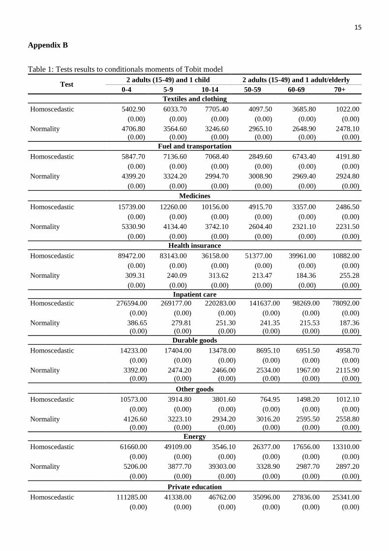
This paper used the CLAD approach to estimate censored models instead of Tobit models. Tobit

models are usually adequate for dependent variables presenting normal and homoscedastic distributions. The test results regarding Tobit estimations rejected the null hypothesis that the data come from a normally

distributed population (Appendix B). Table 1 of Appendix B shows that Tobit estimations presented

heteroscedastic and non-normal distribution of errors, resulting in inconsistent estimated parameters

(Wooldridge, 2000; Cameron and Trivedi, 2005; Powell, 1984). According to Wilhelm (2008) when

heteroscedasticity or non-normality cause bias, CLAD model proposed by Powell (1984) is the best

alternative to the censored regression. Given the large number of models (78 differ models), this section

focus on the main results concerning the coefficients of the six household dummies. Full results are reported

in Appendix C8. All estimations were implemented using Stata 11 software.

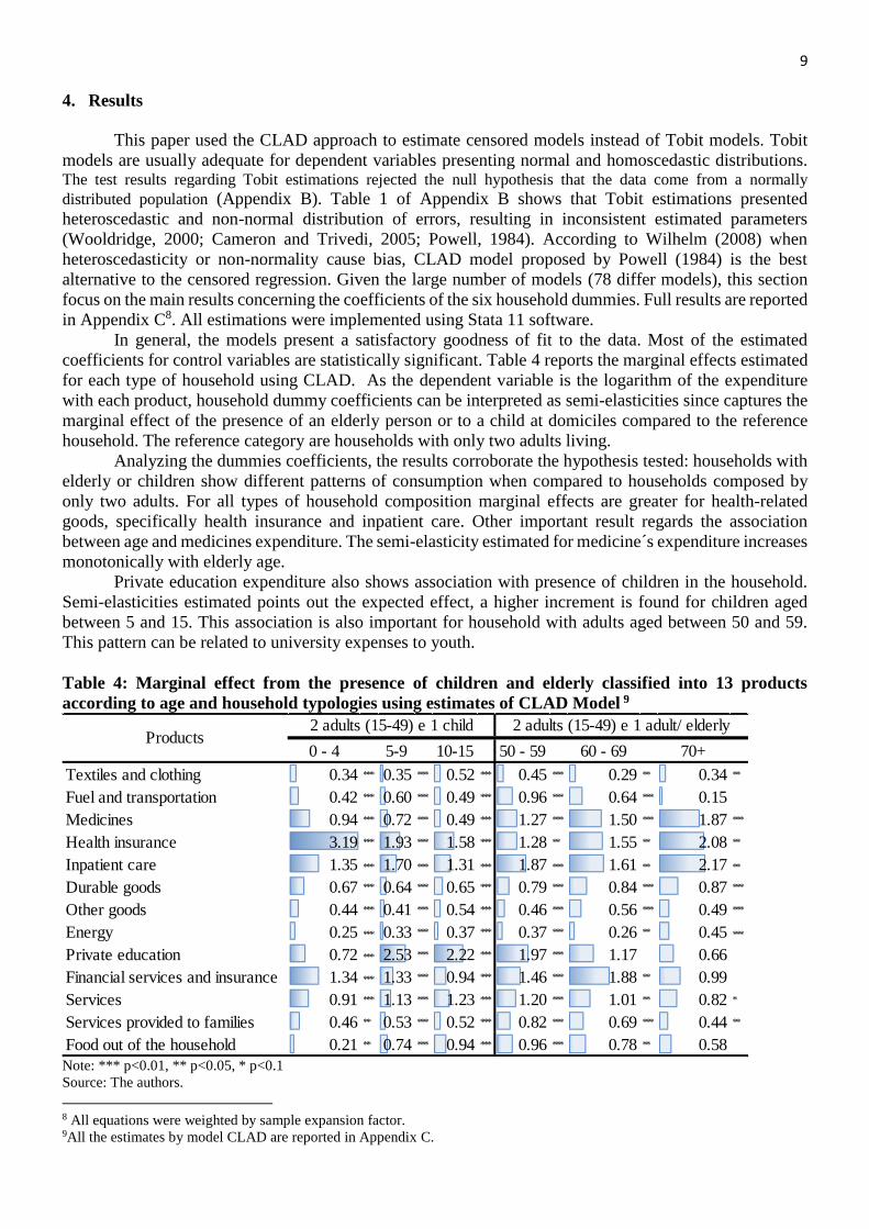
In general, the models present a satisfactory goodness of fit to the data. Most of the estimated

coefficients for control variables are statistically significant. Table 4 reports the marginal effects estimated

for each type of household using CLAD. As the dependent variable is the logarithm of the expenditure

with each product, household dummy coefficients can be interpreted as semi-elasticities since captures the

marginal effect of the presence of an elderly person or to a child at domiciles compared to the reference

household. The reference category are households with only two adults living.

Analyzing the dummies coefficients, the results corroborate the hypothesis tested: households with

elderly or children show different patterns of consumption when compared to households composed by

only two adults. For all types of household composition marginal effects are greater for health-related

goods, specifically health insurance and inpatient care. Other important result regards the association

between age and medicines expenditure. The semi-elasticity estimated for medicine´s expenditure increases

monotonically with elderly age.

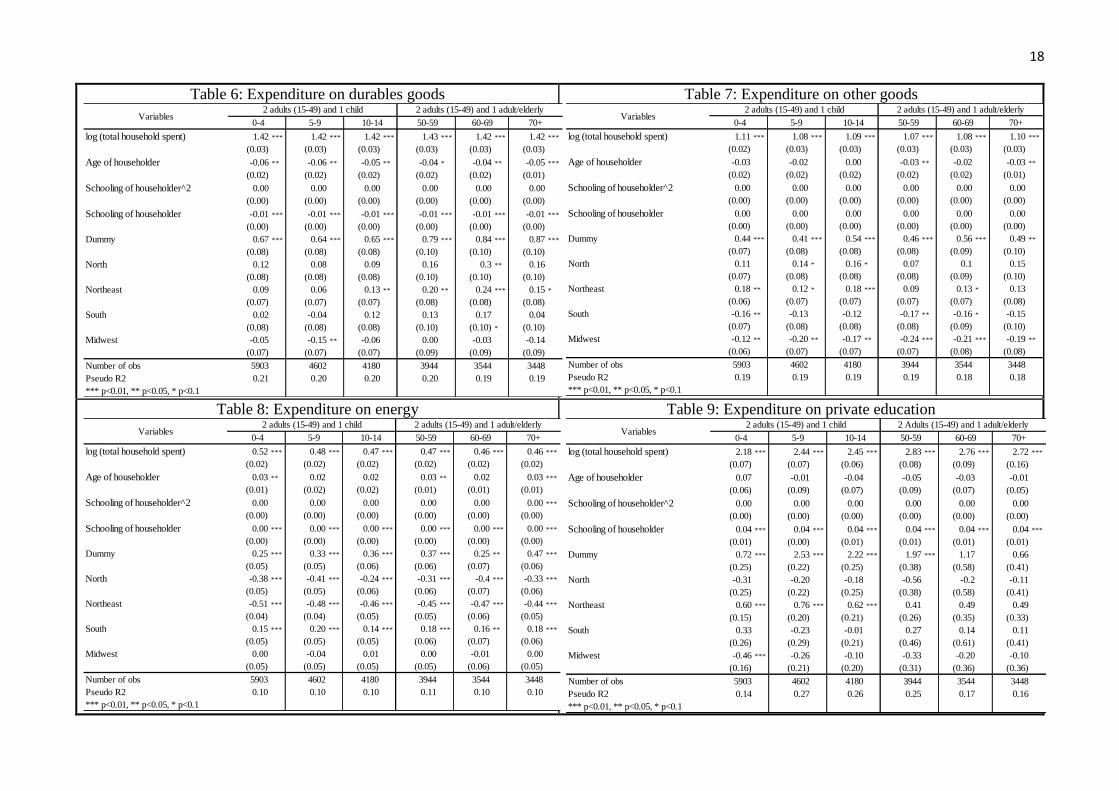
Private education expenditure also shows association with presence of children in the household.

Semi-elasticities estimated points out the expected effect, a higher increment is found for children aged

between 5 and 15. This association is also important for household with adults aged between 50 and 59.

This pattern can be related to university expenses to youth.

Table 4: Marginal effect from the presence of children and elderly classified into 13 products

according to age and household typologies using estimates of CLAD Model 9

Note: *** p<0.01, ** p<0.05, * p<0.1


8 All equations were weighted by sample expansion factor. 9All the estimates by model CLAD are reported in Appendix C.

0 - 4 5-9 10-15 50 - 59 60 - 69 70+

Textiles and clothing 0.34 *** 0.35 *** 0.52 *** 0.45 *** 0.29 ** 0.34 **

Fuel and transportation 0.42 *** 0.60 *** 0.49 *** 0.96 *** 0.64 *** 0.15

Medicines 0.94 *** 0.72 *** 0.49 *** 1.27 *** 1.50 *** 1.87 ***

Health insurance 3.19 *** 1.93 *** 1.58 *** 1.28 ** 1.55 ** 2.08 **

Inpatient care 1.35 *** 1.70 *** 1.31 *** 1.87 *** 1.61 ** 2.17 **

Durable goods 0.67 *** 0.64 *** 0.65 *** 0.79 *** 0.84 *** 0.87 ***

Other goods 0.44 *** 0.41 *** 0.54 *** 0.46 *** 0.56 *** 0.49 ***

Energy 0.25 *** 0.33 *** 0.37 *** 0.37 *** 0.26 ** 0.45 ***

Private education 0.72 *** 2.53 *** 2.22 *** 1.97 *** 1.17 0.66

Financial services and insurance 1.34 *** 1.33 *** 0.94 *** 1.46 *** 1.88 ** 0.99

Services 0.91 *** 1.13 *** 1.23 *** 1.20 *** 1.01 ** 0.82 *

Services provided to families 0.46 ** 0.53 *** 0.52 *** 0.82 *** 0.69 *** 0.44 **

Food out of the household 0.21 ** 0.74 *** 0.94 *** 0.96 *** 0.78 ** 0.58

Products2 adults (15-49) e 1 child 2 adults (15-49) e 1 adult/ elderly

10

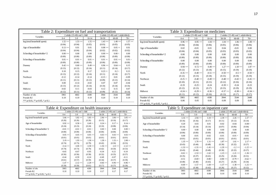
Concerning medicines expenditure (third row of Table 4), it is observed that the presence of one

elderly persons aged over 70 increases this annual expenditure in 187% compared to households with only

two adults living. A smaller effect is also found for the presence of children in households. For households

with two adults and one child, independently of child age, the coefficient is always higher than zero and

significant. Besides there is a child age effect on household expenditure on medicines. Child growth reduces

the needs of medicines as their immunological is more developed. The coefficient decreases as the child

age increases, showing that there is life-cycle effect on this type of expenditure. For households with the

presence of one child aged between 0-4 years this coefficient is 0.94, decreasing to 0.72 for the presence of

a child aged between 5-9 years and to 0.49 for the presence of a child aged between 10-14 years.

With respect to health insurance expenditure (Table 4), the magnitude of the effect associated to the

presence of children and elderly individuals is very high. The presence of one child aged between 0-4 years

increases the health insurance expenditure in 319% compared to households with two adults while the

presence of an elderly person aged over 70 increases this type of expenditure in 208%. An age effect is also

observed for this type of health expenditure. Estimated semi-elasticities present a well-behaved pattern, the

U-curve. It starts with a high effect for children aged 0-4 (319%), after decreases as child age increases and

then increases with age of elderly individuals.

The expenditure effect associated to inpatient care is also important mainly to households with

elderly person aged over 70. In these households this expenditure increases by 217 % when compared to

households composed of only two adults (Table 4). Despite this significant association, age effect on

inpatient care expenses is not well behaved as it was observed for other types of healthcare expenditure. In

this case the U-shaped curve is not observed. This different pattern is probably related to acute events that

occur independently of age.

5. Conclusion

This paper investigated the empirical relationship between household expenditure composition and

the presence of children and elderly individuals in households of Brazil. For this, it was proposed a

methodology to disaggregate the consumer expenditure by age groups using the Consumer Expenditure

Survey (2002-2003). As the information of Consumer Expenditure Survey of Brazil is aggregated by

households, the CLAD model was used to capture the marginal effects of each age group (adults, elderly,

and children) in household expenditure.

Similar to what other studies (e.g. Luhrmann, 2005; Dewhurst, 2006, Lefèbvre, 2006; Almeida,

2002; Zanon, 2012), the results showed that changes in the age structure of the population have significant

effects on Brazilian aggregate consumption. The results obtained in the econometric model revealed

different consumption patterns depending on the household type.

Analyzing the dummies coefficients, the results showed that the presence of children and elderly

individuals changed the consumption pattern resulting in different budget allocation favoring healthcare

expenditure. For the healthcare categories expenditure, semi-elasticities increased monotonically with age.

The results also showed that expenditures on medicines are more important for extreme age groups, which

means in the age group between zero and four years old and in the age group for persons 70 years old or

more.

This paper is the first attempt to estimate effects of changing population age structure over

consumption profiles. Results showed that aging can affect aggregate demand through changes in

consumption pattern. The parameters estimated in this paper can subsidize public policy and planning of

healthcare supply and other goods and services.

Acknowledgements

We would like to thank Professor Mark Ottoni-Wilhelmor who kindly provided his files to simulate the

marginal effects of CLAD model.

11

References

ALMEIDA, A. N. Determinantes do consumo de famílias com idosos e sem idosos com base na pesquisa

de orçamentos familiares 1995/96. 2002. 109 p. Dissertação (Mestrado em Ciências) - Escola Superior

de Agricultura Luiz de Queiroz, Universidade de São Paulo, Piracicaba, 2002.

ANDRADE, M. V., NORONHA, K. M. S., OLIVEIRA, T. Determinantes dos Gastos das Famílias com

Saúde no Brasil. Economia. v.7, n.3, p.485–508, set./dez. 2006.

ALVES, J.E.D.A. A transição demográfica e a janela de oportunidades. Instituto Fernand Braudel de

Economia Mundial. São Paulo, 2008.

BUCHINSKY, M. Changes in the US wage structure 1963-1987: application of quantile regression,

Econometrica, v. 2, p. 405-458, 1994.

CAMERON, C.A., TRIVEDI, K.P. Microeconometrics: Methods and Applications. Cambridge University

Press, 2005.

CAMERON, C.A., TRIVEDI, K.P. Micro econometrics Using Stata. College Station, Texas: Stata Press,

2009.

DEATON, A. The analysis of household surveys: a microeconometric approach to development policy.

Johns Hopkins, 1997.

DENTON, F.T., SPENCER, B.G. Population Aging and Its Economic Costs: A Survey of Issues and

Evidences. SEDAP Research Paper, v. 1. McMaster University, Hamilton, 1999.

DEWHURST, J. H. L. Estimating the Effect of Projected Household Composition Change on Production

in Scotland. University of Dundee, Department of Economic Studies, 2006. (Working Paper, 186).

FOUGÈRE, M.; MERCENIER, J.; MÉRETTE, M. A sectoral and occupational analysis of population

ageing in Canada using a dynamic CGE overlapping generations model. Economic Modelling, v. 24,

n.4, p. 690-711, jul. 2007.

IBGE - Instituto Brasileiro de Geografia e Estatística - Pesquisa de Orçamento das Famílias (POF 2003-

2004). Instituto Brasileiro de Geografia e Estatística (IBGE), 2004. Disponível em<

http://www.ibge.gov.br/home/estatistica/populacao/pof/2002_2003>. Acesso em 17 abr. 2011.

KIM, k.; KRATENA, K.; HEWINGS, G. The Extended Econometric Input-Output model with

Heterogeneous Household Demand System. Economic Systems Research, v.27, n. 2, p. 257-285, dec.

2015.

KOENKER, R.; BASSETT, G. Jr. Regression Quantiles. Econornetrica, v. 46, n. 1, p. 33-50, 1978.

PAIVA, P., T., A.; WAJNMAN, S. Das causas às consequências econômicas da transição demográfica no

Brasil. Revista Brasileira de Estudos de População, v. 22, n. 2, p. 303-322, jul./dez. 2005.

PAGAN, A.; VELLA, F. Diagnostic tests for models based on individual data: a survey, Journal of Applied

Econometrics, Vol. 4, p.29–59, 1989.

POWELL, J. Least absolute deviations estimation for censored regression model. Journal of Econometrics,

v. 32, p. 143-155, 1984.

POWELL, J. L. Symmetrically trimmed least squares estimation for Tobit models, Econometrica, v. 54, p.

1435-1460, 1986.

LEFÈBVRE, M. Population Ageing and Consumption Demand in Belgium. CREPP – University of Liège,

2006. 20 p. (Working papers, 0604).

LÜHRMANN, M. Population Aging and the Demand for Goods & Services. Universität Mannheim: MEA

- Mannheim Research Institute for the Economics of Aging,/ Department of Economics, 2005.

(Discussion paper, D-68131).

NERI, M. et al. Inflação e os idosos brasileiros. In: CAMARANO, A. A. (org.). Os Novos Idosos

Brasileiros: muito além dos 60? Rio de Janeiro, IPEA, 2004. 604p.

SASSI, M. R, BÉRIA, J. U. Utilización de los servicios de salud: una revisión sistemática sobre los factores

relacionados. Cadernos de Saúde Pública, v.17, n.4, p.819-832, jul/ago, 2001.

TOBIN, J. Estimation of relationships for limited dependent variables. Econometrica, v. 26, p. 24-36, 1958.

12

UNITED NATIONS, Department of Economic and Social Affairs, Population Division (2011). World

Population Prospects: The 2010 Revision. Available in: <http://go.worldbank.org/KZHE1CQFA0>.

Accessed on 02 mar. 2012.

WILHELM, M. O. Practical Considerations for Choosing Between Tobit and SCLS or CLAD Estimators

for Censored Regression Models with an Application to Charitable Giving. Oxford Bulletin of

Economics and Statistics, v.70, n.4, p.559-582, 2008.

WOOLDRIDGE, J. M. Introductory econometrics: a modern approach. Cincinnati, OH, South-West,

2000.

YOON, S.G; HEWINGS, G.J.D. Impacts of Demographic Changes in the Chicago Region. Regional

Economics Applications Laboratory/ University of Illinois, 41p. 2006. (Discussion paper, REAL 06-

T-7)

ZANON, R. R. Envelhecimento populacional e mudanças no padrão de consumo: impactos na estrutura

produtiva do Brasil. 2012. 79p. Dissertação (Mestrado em Economia Regional) - Programa de Pós-

Graduação em Economia Regional, Universidade Estadual de Londrina, Centro de Estudos Sociais

Aplicados, 2012.

http://go.worldbank.org/KZHE1CQFA0

13

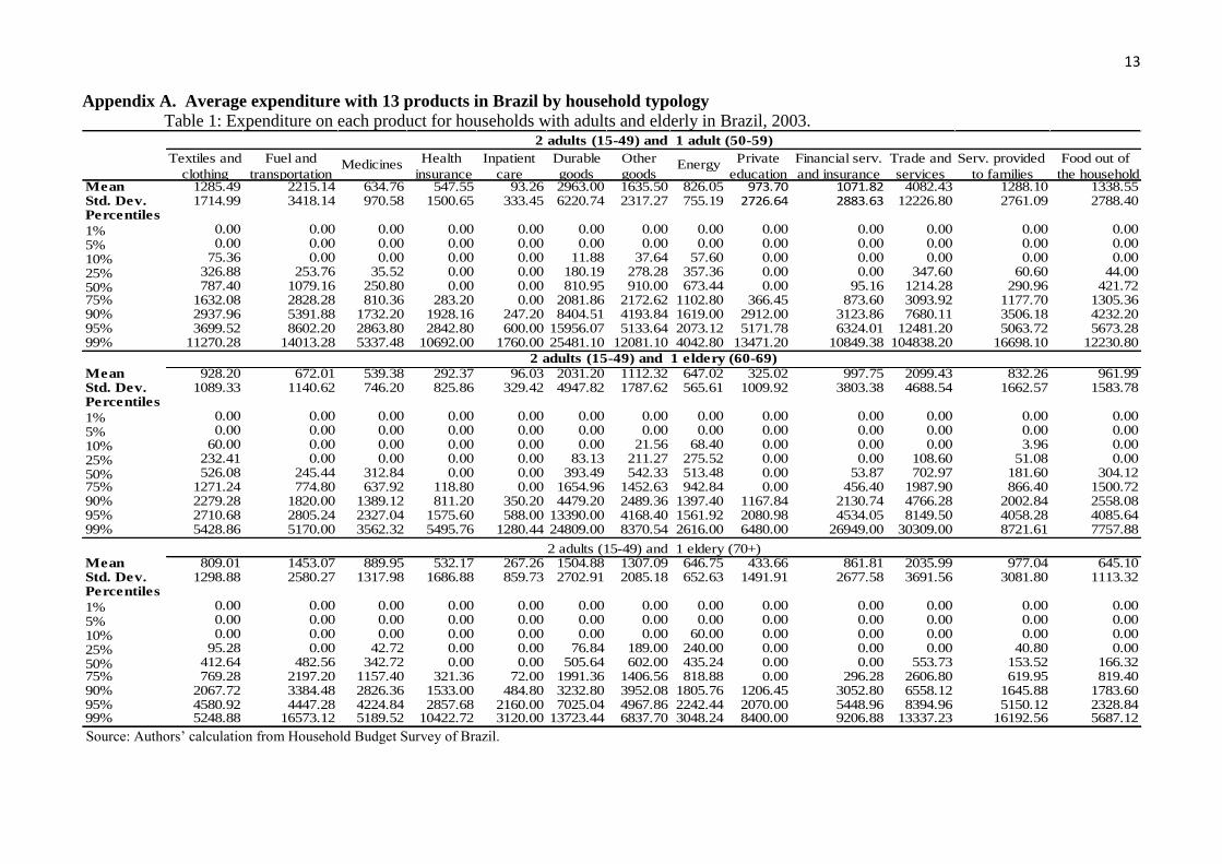
Appendix A. Average expenditure with 13 products in Brazil by household typology

Table 1: Expenditure on each product for households with adults and elderly in Brazil, 2003.

Source: Authors’ calculation from Household Budget Survey of Brazil.

Textiles and Fuel and Health Inpatient Durable Other Private Financial serv. Trade and Serv. provided Food out of

clothing transportation insurance care goods goods education and insurance services to families the householdMean 1285.49 2215.14 634.76 547.55 93.26 2963.00 1635.50 826.05 973.70 1071.82 4082.43 1288.10 1338.55Std. Dev. 1714.99 3418.14 970.58 1500.65 333.45 6220.74 2317.27 755.19 2726.64 2883.63 12226.80 2761.09 2788.40Percentiles

1% 0.00 0.00 0.00 0.00 0.00 0.00 0.00 0.00 0.00 0.00 0.00 0.00 0.00

5% 0.00 0.00 0.00 0.00 0.00 0.00 0.00 0.00 0.00 0.00 0.00 0.00 0.00

10% 75.36 0.00 0.00 0.00 0.00 11.88 37.64 57.60 0.00 0.00 0.00 0.00 0.00

25% 326.88 253.76 35.52 0.00 0.00 180.19 278.28 357.36 0.00 0.00 347.60 60.60 44.00

50% 787.40 1079.16 250.80 0.00 0.00 810.95 910.00 673.44 0.00 95.16 1214.28 290.96 421.7275% 1632.08 2828.28 810.36 283.20 0.00 2081.86 2172.62 1102.80 366.45 873.60 3093.92 1177.70 1305.3690% 2937.96 5391.88 1732.20 1928.16 247.20 8404.51 4193.84 1619.00 2912.00 3123.86 7680.11 3506.18 4232.2095% 3699.52 8602.20 2863.80 2842.80 600.00 15956.07 5133.64 2073.12 5171.78 6324.01 12481.20 5063.72 5673.2899% 11270.28 14013.28 5337.48 10692.00 1760.00 25481.10 12081.10 4042.80 13471.20 10849.38 104838.20 16698.10 12230.80

Mean 928.20 672.01 539.38 292.37 96.03 2031.20 1112.32 647.02 325.02 997.75 2099.43 832.26 961.99Std. Dev. 1089.33 1140.62 746.20 825.86 329.42 4947.82 1787.62 565.61 1009.92 3803.38 4688.54 1662.57 1583.78Percentiles

1% 0.00 0.00 0.00 0.00 0.00 0.00 0.00 0.00 0.00 0.00 0.00 0.00 0.00

5% 0.00 0.00 0.00 0.00 0.00 0.00 0.00 0.00 0.00 0.00 0.00 0.00 0.00

10% 60.00 0.00 0.00 0.00 0.00 0.00 21.56 68.40 0.00 0.00 0.00 3.96 0.00

25% 232.41 0.00 0.00 0.00 0.00 83.13 211.27 275.52 0.00 0.00 108.60 51.08 0.00

50% 526.08 245.44 312.84 0.00 0.00 393.49 542.33 513.48 0.00 53.87 702.97 181.60 304.1275% 1271.24 774.80 637.92 118.80 0.00 1654.96 1452.63 942.84 0.00 456.40 1987.90 866.40 1500.7290% 2279.28 1820.00 1389.12 811.20 350.20 4479.20 2489.36 1397.40 1167.84 2130.74 4766.28 2002.84 2558.0895% 2710.68 2805.24 2327.04 1575.60 588.00 13390.00 4168.40 1561.92 2080.98 4534.05 8149.50 4058.28 4085.6499% 5428.86 5170.00 3562.32 5495.76 1280.44 24809.00 8370.54 2616.00 6480.00 26949.00 30309.00 8721.61 7757.88


1% 0.00 0.00 0.00 0.00 0.00 0.00 0.00 0.00 0.00 0.00 0.00 0.00 0.00

5% 0.00 0.00 0.00 0.00 0.00 0.00 0.00 0.00 0.00 0.00 0.00 0.00 0.00

10% 0.00 0.00 0.00 0.00 0.00 0.00 0.00 60.00 0.00 0.00 0.00 0.00 0.00

25% 95.28 0.00 42.72 0.00 0.00 76.84 189.00 240.00 0.00 0.00 0.00 40.80 0.00

50% 412.64 482.56 342.72 0.00 0.00 505.64 602.00 435.24 0.00 0.00 553.73 153.52 166.3275% 769.28 2197.20 1157.40 321.36 72.00 1991.36 1406.56 818.88 0.00 296.28 2606.80 619.95 819.4090% 2067.72 3384.48 2826.36 1533.00 484.80 3232.80 3952.08 1805.76 1206.45 3052.80 6558.12 1645.88 1783.6095% 4580.92 4447.28 4224.84 2857.68 2160.00 7025.04 4967.86 2242.44 2070.00 5448.96 8394.96 5150.12 2328.8499% 5248.88 16573.12 5189.52 10422.72 3120.00 13723.44 6837.70 3048.24 8400.00 9206.88 13337.23 16192.56 5687.12

2 adults (15-49) and 1 adult (50-59)

2 adults (15-49) and 1 eldery (60-69)

2 adults (15-49) and 1 eldery (70+)

Medicines Energy

14

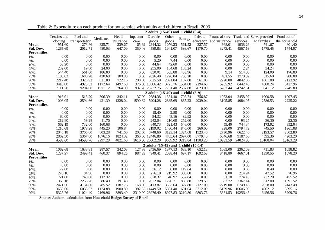
Table 2: Expenditure on each product for households with adults and children in Brazil, 2003.

Source: Authors’ calculation from Household Budget Survey of Brazil.

Textiles and Fuel and Health Inpatient Durable Other Private Financial serv. Trade and Serv. provided Food out of

clothing transportation insurance care goods goods education and insurance services to families the householdMean 951.60 1278.86 325.71 239.67 65.89 2344.32 1076.23 561.52 327.57 968.01 1938.26 741.67 801.40Std. Dev. 1265.69 2012.71 480.03 647.09 350.46 4589.83 1941.07 586.67 1179.70 3273.41 4567.16 1775.45 1744.07Percentiles

1% 0.00 0.00 0.00 0.00 0.00 0.00 0.00 0.00 0.00 0.00 0.00 0.00 0.00

5% 0.00 0.00 0.00 0.00 0.00 5.20 7.44 0.00 0.00 0.00 0.00 0.00 0.00

10% 58.20 0.00 0.00 0.00 0.00 44.64 42.60 0.00 0.00 0.00 0.00 0.00 0.00

25% 232.00 19.80 24.00 0.00 0.00 255.00 184.68 183.24 0.00 0.00 2.24 34.24 0.00

50% 544.40 561.60 186.00 0.00 0.00 830.01 563.88 453.96 0.00 9.14 514.80 124.00 176.8075% 1180.02 1686.28 430.68 100.80 0.00 2026.40 1226.04 730.20 0.00 481.55 1770.32 515.60 906.8890% 2217.48 3325.92 821.88 722.16 200.00 5825.58 2691.84 1187.88 561.00 2220.00 4842.06 1861.80 2123.9295% 3416.00 4925.52 1172.64 1497.60 376.00 10586.42 3723.76 1594.08 2194.68 5235.92 8442.40 4308.24 3427.9699% 7111.20 9204.00 1971.12 3264.00 937.28 25232.75 7751.40 2537.88 7623.00 15783.44 24242.61 8541.12 7245.80


1% 0.00 0.00 0.00 0.00 0.00 0.00 0.00 0.00 0.00 0.00 0.00 0.00 0.00

5% 0.00 0.00 0.00 0.00 0.00 15.40 2.80 0.00 0.00 0.00 0.00 0.00 0.00

10% 60.00 0.00 0.00 0.00 0.00 54.32 45.16 82.92 0.00 0.00 0.00 0.00 0.00

25% 212.80 59.28 11.76 0.00 0.00 242.04 216.60 252.60 0.00 0.00 93.25 36.36 22.36

50% 662.19 732.00 160.68 0.00 0.00 840.73 621.43 546.00 0.00 59.40 744.34 173.92 352.0475% 1210.08 1978.28 445.20 106.84 0.00 2199.02 1460.44 840.00 360.00 828.00 2794.72 745.50 1361.8890% 2046.18 3705.00 803.28 741.60 202.00 6748.60 3123.14 1324.68 1523.40 2730.96 6622.46 2193.57 2802.8095% 2862.30 5367.60 1076.16 1824.32 360.00 12446.80 4703.64 2097.00 3779.40 5046.68 9187.56 4595.36 4203.2099% 4589.60 14593.76 2297.28 4821.60 1616.00 26002.28 9659.92 3219.84 11383.20 10933.59 24824.80 16108.04 13163.28


1% 0.00 0.00 0.00 0.00 0.00 0.00 0.00 0.00 0.00 0.00 0.00 0.00 0.00

5% 0.00 0.00 0.00 0.00 0.00 0.00 0.00 0.00 0.00 0.00 0.00 0.00 0.00

10% 72.00 0.00 0.00 0.00 0.00 36.12 50.88 119.64 0.00 0.00 0.00 8.40 0.00

25% 276.16 84.96 0.00 0.00 0.00 276.10 219.92 300.60 0.00 0.00 214.24 47.52 76.96

50% 721.80 748.80 112.32 0.00 0.00 878.37 640.97 552.84 0.00 51.10 774.10 222.20 455.5275% 1365.18 2255.76 386.40 191.48 0.00 2072.04 1720.21 860.88 229.50 662.72 2367.14 612.00 1391.5290% 2471.56 4154.80 785.52 1187.76 168.00 6113.87 3563.64 1327.80 2127.00 2719.00 6749.18 2078.00 2443.4895% 3635.60 6035.52 1124.88 1900.80 382.32 11449.50 5081.40 1691.04 3712.00 5139.96 10606.00 4002.12 3895.1699% 5325.76 11024.40 2169.96 3893.40 2310.00 23976.40 8927.83 3210.80 9803.76 15381.53 19256.45 6456.56 8209.76

2 adults (15-49) and 1 child (10-14)

2 adults (15-49) and 1 child (0-4)

2 adults (15-49) and 1 child (5-9)

Medicines Energy

15

Appendix B

Table 1: Tests results to conditionals moments of Tobit model

Test 2 adults (15-49) and 1 child 2 adults (15-49) and 1 adult/elderly

0-4 5-9 10-14 50-59 60-69 70+

Textiles and clothing

Homoscedastic 5402.90 6033.70 7705.40 4097.50 3685.80 1022.00

(0.00) (0.00) (0.00) (0.00) (0.00) (0.00)

Normality 4706.80 3564.60 3246.60 2965.10 2648.90 2478.10

(0.00) (0.00) (0.00) (0.00) (0.00) (0.00)

Fuel and transportation

Homoscedastic 5847.70 7136.60 7068.40 2849.60 6743.40 4191.80

(0.00) (0.00) (0.00) (0.00) (0.00) (0.00)

Normality 4399.20 3324.20 2994.70 3008.90 2969.40 2924.80

(0.00) (0.00) (0.00) (0.00) (0.00) (0.00)

Medicines

Homoscedastic 15739.00 12260.00 10156.00 4915.70 3357.00 2486.50

(0.00) (0.00) (0.00) (0.00) (0.00) (0.00)

Normality 5330.90 4134.40 3742.10 2604.40 2321.10 2231.50

(0.00) (0.00) (0.00) (0.00) (0.00) (0.00)

Health insurance

Homoscedastic 89472.00 83143.00 36158.00 51377.00 39961.00 10882.00

(0.00) (0.00) (0.00) (0.00) (0.00) (0.00)

Normality 309.31 240.09 313.62 213.47 184.36 255.28

(0.00) (0.00) (0.00) (0.00) (0.00) (0.00)

Inpatient care

Homoscedastic 276594.00 269177.00 220283.00 141637.00 98269.00 78092.00

(0.00) (0.00) (0.00) (0.00) (0.00) (0.00)

Normality 386.65 279.81 251.30 241.35 215.53 187.36

(0.00) (0.00) (0.00) (0.00) (0.00) (0.00)

Durable goods

Homoscedastic 14233.00 17404.00 13478.00 8695.10 6951.50 4958.70

(0.00) (0.00) (0.00) (0.00) (0.00) (0.00)

Normality 3392.00 2474.20 2466.00 2534.00 1967.00 2115.90

(0.00) (0.00) (0.00) (0.00) (0.00) (0.00)

Other goods

Homoscedastic 10573.00 3914.80 3801.60 764.95 1498.20 1012.10

(0.00) (0.00) (0.00) (0.00) (0.00) (0.00)

Normality 4126.60 3223.10 2934.20 3016.20 2595.50 2558.80

(0.00) (0.00) (0.00) (0.00) (0.00) (0.00)

Energy

Homoscedastic 61660.00 49109.00 3546.10 26377.00 17656.00 13310.00

(0.00) (0.00) (0.00) (0.00) (0.00) (0.00)

Normality 5206.00 3877.70 39303.00 3328.90 2987.70 2897.20

(0.00) (0.00) (0.00) (0.00) (0.00) (0.00)

Private education

Homoscedastic 111285.00 41338.00 46762.00 35096.00 27836.00 25341.00

(0.00) (0.00) (0.00) (0.00) (0.00) (0.00)

16

Test 2 adults (15-49) and 1 child 2 adults (15-49) and 1 adult/elderly

0-4 5-9 10-14 50-59 60-69 70+

Normality 318.91 258.65 222.76 233.01 234.91 202.33

(0.00) (0.00) (0.00) (0.00) (0.00) (0.00)

Financial services and insurance

Homoscedastic 32361.00 21136.00 21408.00 13717.00 10831 5536.90

(0.00) (0.00) (0.00) (0.00) (0.00) (0.00)

Normality 302.47 272.81 256.18 235.00 200.05 203.33

(0.00) (0.00) (0.00) (0.00) (0.00) (0.00)

Services

Homoscedastic 5662.50 6936.00 21286.00 6184.30 6185.20 2782.40

(0.00) (0.00) (0.00) (0.00) (0.00) (0.00)

Normality 1753.90 1671.50 1671.50 1599.40 1482.40 1455.90

(0.00) (0.00) (0.00) (0.00) (0.00) (0.00)

Services provided to families

Homoscedastic 6751.00 4939.90 4755.30 1038.20 2090.20 2199.20

(0.00) (0.00) (0.00) (0.00) (0.00) (0.00)

Normality 2639.00 1994.80 1469.40 2195.80 1811.20 1726.20

(0.00) (0.00) (0.00) (0.00) (0.00) (0.00)

Food out of the household

Homoscedastic 9877.30 8063.90 10519.00 2690.40 2401.50 1089.10

(0.00) (0.00) (0.00) (0.00) (0.00) (0.00)

Normality 3542.30 2457.90 2199.90 2066.70 1649.40 1723.80

(0.00) (0.00) (0.00) (0.00) (0.00) (0.00)


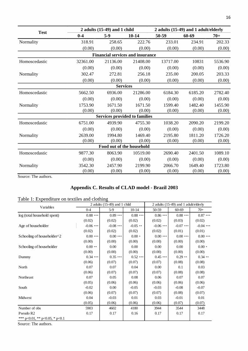
Appendix C. Results of CLAD model - Brazil 2003

Table 1: Expenditure on textiles and clothing


log (total household spent) 0.88 *** 0.89 *** 0.88 *** 0.86 *** 0.88 *** 0.87 ***

(0.02) (0.02) (0.02) (0.02) (0.03) (0.02)

Age of householder -0.06 *** -0.08 *** -0.05 ** -0.06 *** -0.07 *** -0.04 ***

(0.02) (0.02) (0.02) (0.02) (0.01) (0.01)

Schooling of householder^2 0.00 *** 0.00 *** 0.00 * 0.00 *** 0.00 *** 0.00 ***

(0.00) (0.00) (0.00) (0.00) (0.00) (0.00)

Schooling of householder 0.00 ** 0.00 0.00 0.00 0.00 0.00 *

(0.00) (0.00) (0.00) (0.00) (0.00) (0.00)

Dummy 0.34 *** 0.35 *** 0.52 *** 0.45 *** 0.29 ** 0.34 **

(0.06) (0.07) (0.07) (0.07) (0.08) (0.08)

North 0.07 0.07 0.04 0.00 0.1 0.03

(0.06) (0.07) (0.07) (0.07) (0.08) (0.08)

Northeast 0.07 0.05 0.08 0.06 0.07 0.07

(0.05) (0.06) (0.06) (0.06) (0.06) (0.06)

South -0.02 0.00 -0.05 -0.03 -0.08 -0.07

(0.06) (0.07) (0.07) (0.07) (0.08) (0.07)

Midwest 0.04 -0.03 0.01 0.03 -0.01 0.01

(0.05) (0.06) (0.06) (0.06) (0.07) (0.07)

Number of obs 5903 4602 4180 3944 3544 3448

Pseudo R2 0.17 0.17 0.16 0.17 0.17 0.17

*** p<0.01, ** p<0.05, * p<0.1

Variables2 adults (15-49) and 1 child 2 adults (15-49) and 1 adult/elderly

0-4 5-9 10-14 50-59 60-69 70+

17

Table 2: Expenditure on fuel and transportation

Table 3: Expenditure on medicines

Table 4: Expenditure on health insurance

Table 5: Expenditure on inpatient care


(0.04) (0.04) (0.05) (0.03) (0.05) (0.05)

Age of householder 0.13 *** 0.01 0.01 0.08 *** 0.05 ** 0.01

(0.04) (0.04) (0.04) (0.02) (0.02) (0.02)

Schooling of householder^2 0.00 *** 0.00 0.00 0.00 *** 0.00 * 0.00

(0.00) (0.00) (0.00) (0.00) (0.00) (0.00)

Schooling of householder 0.01 ** 0.01 ** 0.01 ** 0.01 ** 0.01 *** 0.01 *

(0.00) (0.00) (0.00) (0.00) (0.00) (0.00)

Dummy 0.42 *** 0.60 *** 0.49 *** 0.96 *** 0.64 *** 0.15

(0.13) (0.12) (0.14) (0.11) (0.14) (0.17)

North 0.10 0.15 0.17 0.23 ** 0.2 * 0.15

(0.13) (0.12) (0.14) (0.11) (0.14) (0.17)

Northeast -0.12 -0.14 -0.14 -0.15 * 0.01 -0.09

(0.11) (0.11) (0.12) (0.09) (0.12) (0.14)

South 0.00 -0.14 -0.02 0.07 0.07 -0.04

(0.13) (0.12) (0.14) (0.10) (0.14) (0.16)

Midwest -0.02 0.11 -0.03 0.12 0.15 0.07

(0.12) (0.11) (0.12) (0.09) (0.12) (0.14)

Number of obs 5903 4602 4180 3944 3544 3448

Pseudo R2 0.19 0.19 0.19 0.20 0.19 0.19

*** p<0.01, ** p<0.05, * p<0.1


0-4 5-9 10-14 50-59 60-69 70+


(0.04) (0.04) (0.06) (0.05) (0.06) (0.06)

Age of householder 0.02 -0.01 0.01 0.04 -0.01 0.00

(0.04) (0.04) (0.05) (0.03) (0.03) (0.02)

Schooling of householder^2 0.00 0.00 0.00 0.00 0.00 0.00

(0.00) (0.00) (0.00) (0.00) (0.00) (0.00)

Schooling of householder 0.00 0.00 0.00 0.00 0.00 0.00

(0.00) (0.00) (0.00) (0.00) (0.00) (0.00)

Dummy 0.94 *** 0.72 *** 0.49 *** 1.27 *** 1.50 *** 1.87 ***

(0.12) (0.13) (0.18) (0.15) (0.19) (0.19)

North -0.35 *** -0.40 *** -0.51 *** -0.50 *** -0.5 ** -0.50 **

(0.12) (0.13) (0.18) (0.15) (0.19) (0.19)

Northeast -0.25 ** -0.40 *** -0.49 *** -0.48 *** -0.43 ** -0.45 ***

(0.10) (0.11) (0.15) (0.12) (0.16) (0.16)

South -0.19 -0.25 * -0.24 -0.39 ** -0.24 -0.23

(0.12) (0.13) (0.17) (0.15) (0.19) (0.19)

Midwest -0.24 ** -0.29 ** -0.36 ** -0.37 *** -0.38 ** -0.34 **

(0.11) (0.12) (0.16) (0.13) (0.17) (0.17)

Number of obs 5903 4602 4180 3944 3544 3448

Pseudo R2 0.06 0.05 0.05 0.09 0.09 0.09

*** p<0.01, ** p<0.05, * p<0.1


0-4 5-9 10-14 50-59 60-69 70+


(0.26) (0.26) (0.26) (0.15) (0.16) (0.17)

Age of householder 0.92 *** 0.58 ** 0.49 ** 0.24 ** 0.17 ** 0.14 **

(0.24) (0.23) (0.24) (0.10) (0.08) (0.06)

Schooling of householder^2 -0.01 *** -0.01 ** -0.01 * 0.00 ** 0.00 0.00 **

(0.00) (0.00) (0.00) (0.00) (0.00) (0.00)

Schooling of householder 0.05 *** 0.05 *** 0.05 *** 0.03 *** 0.03 *** 0.03 ***

(0.01) (0.01) (0.01) (0.01) (0.01) (0.01)

Dummy 3.19 *** 1.93 *** 1.58 *** 1.28 ** 1.55 ** 2.08 **

(0.74) (0.73) (0.79) (0.42) (0.50) (0.53)

North -3.14 *** -3.06 *** -3.58 *** -1.36 *** -2.0 *** -2.12 ***

(0.74) (0.73) (0.79) (0.42) (0.50) (0.53)

Northeast -0.65 -0.67 -0.95 -0.34 -0.21 -0.10

(0.56) (0.56) (0.58) (0.32) (0.35) (0.37)

South -0.44 -0.59 -0.24 -0.40 -0.07 -0.11

(0.61) (0.57) (0.59) (0.34) (0.37) (0.39)

Midwest -1.47 ** -2.12 *** -2.28 *** -0.66 *** -0.96 *** -0.96 **

(0.59) (0.59) (0.61) (0.17) (0.37) (0.39)

Number of obs 5903 4602 4180 3944 3544 3448

Pseudo R2 0.10 0.10 0.10 0.17 0.17 0.17

*** p<0.01, ** p<0.05, * p<0.1


0-4 5-9 10-14 50-59 60-69 70+


(0.16) (0.16) (0.17) (0.11) (0.12) (0.14)

Age of householder 0.20 0.03 0.01 -0.02 -0.04 -0.08 *

(0.14) (0.14) (0.14) (0.07) (0.06) (0.04)

Schooling of householder^2 0.00 * 0.00 0.00 0.00 0.00 0.00

(0.00) (0.00) (0.00) (0.00) (0.00) (0.00)

Schooling of householder 0.00 -0.01 -0.02 -0.01 -0.01 * -0.01

(0.01) (0.01) (0.01) (0.01) (0.01) (0.01)

Dummy 1.35 *** 1.70 *** 1.31 *** 1.87 *** 1.61 ** 2.17 **

(0.43) (0.44) (0.48) (0.30) (0.32) (0.37)

North -1.33 *** -1.55 *** -1.45 *** -1.20 *** -1.2 *** -1.22 ***

(0.43) (0.44) (0.48) (0.30) (0.32) (0.37)

Northeast -0.61 ** -1.53 *** -1.62 *** -1.23 *** -1.21 *** -1.36 ***

(0.35) (0.37) (0.41) (0.25) (0.26) (0.31)

South -0.51 -0.69 * -0.80 * -0.80 *** -0.79 ** -0.62 **

(0.40) (0.40) (0.43) (0.27) (0.29) (0.34)

Midwest -0.69 ** -1.57 *** -1.69 *** -1.37 *** -1.38 *** -1.25 ***

(0.37) (0.38) (0.42) (0.26) (0.27) (0.32)

Number of obs 5903 4602 4180 3944 3544 3448

Pseudo R2 0.09 0.08 0.08 0.10 0.09 0.10

*** p<0.01, ** p<0.05, * p<0.1


0-4 5-9 10-14 50-59 60-69 70+

18

Table 6: Expenditure on durables goods

Table 7: Expenditure on other goods

Table 8: Expenditure on energy

Table 9: Expenditure on private education


(0.03) (0.03) (0.03) (0.03) (0.03) (0.03)

Age of householder -0.06 ** -0.06 ** -0.05 ** -0.04 * -0.04 ** -0.05 ***

(0.02) (0.02) (0.02) (0.02) (0.02) (0.01)


(0.00) (0.00) (0.00) (0.00) (0.00) (0.00)

Schooling of householder -0.01 *** -0.01 *** -0.01 *** -0.01 *** -0.01 *** -0.01 ***

(0.00) (0.00) (0.00) (0.00) (0.00) (0.00)

Dummy 0.67 *** 0.64 *** 0.65 *** 0.79 *** 0.84 *** 0.87 ***

(0.08) (0.08) (0.08) (0.10) (0.10) (0.10)

North 0.12 0.08 0.09 0.16 0.3 ** 0.16

(0.08) (0.08) (0.08) (0.10) (0.10) (0.10)

Northeast 0.09 0.06 0.13 ** 0.20 ** 0.24 *** 0.15 *

(0.07) (0.07) (0.07) (0.08) (0.08) (0.08)

South 0.02 -0.04 0.12 0.13 0.17 0.04

(0.08) (0.08) (0.08) (0.10) (0.10) * (0.10)

Midwest -0.05 -0.15 ** -0.06 0.00 -0.03 -0.14

(0.07) (0.07) (0.07) (0.09) (0.09) (0.09)

Number of obs 5903 4602 4180 3944 3544 3448

Pseudo R2 0.21 0.20 0.20 0.20 0.19 0.19

*** p<0.01, ** p<0.05, * p<0.1


0-4 5-9 10-14 50-59 60-69 70+


(0.02) (0.03) (0.03) (0.03) (0.03) (0.03)

Age of householder -0.03 -0.02 0.00 -0.03 ** -0.02 -0.03 **

(0.02) (0.02) (0.02) (0.02) (0.02) (0.01)


(0.00) (0.00) (0.00) (0.00) (0.00) (0.00)


(0.00) (0.00) (0.00) (0.00) (0.00) (0.00)

Dummy 0.44 *** 0.41 *** 0.54 *** 0.46 *** 0.56 *** 0.49 **

(0.07) (0.08) (0.08) (0.08) (0.09) (0.10)

North 0.11 0.14 * 0.16 * 0.07 0.1 0.15

(0.07) (0.08) (0.08) (0.08) (0.09) (0.10)

Northeast 0.18 ** 0.12 * 0.18 *** 0.09 0.13 * 0.13

(0.06) (0.07) (0.07) (0.07) (0.07) (0.08)

South -0.16 ** -0.13 -0.12 -0.17 ** -0.16 * -0.15

(0.07) (0.08) (0.08) (0.08) (0.09) (0.10)

Midwest -0.12 ** -0.20 ** -0.17 ** -0.24 *** -0.21 *** -0.19 **

(0.06) (0.07) (0.07) (0.07) (0.08) (0.08)

Number of obs 5903 4602 4180 3944 3544 3448

Pseudo R2 0.19 0.19 0.19 0.19 0.18 0.18

*** p<0.01, ** p<0.05, * p<0.1


0-4 5-9 10-14 50-59 60-69 70+


(0.02) (0.02) (0.02) (0.02) (0.02) (0.02)

Age of householder 0.03 ** 0.02 0.02 0.03 ** 0.02 0.03 ***

(0.01) (0.02) (0.02) (0.01) (0.01) (0.01)

Schooling of householder^2 0.00 0.00 0.00 0.00 0.00 0.00 ***

(0.00) (0.00) (0.00) (0.00) (0.00) (0.00)


(0.00) (0.00) (0.00) (0.00) (0.00) (0.00)

Dummy 0.25 *** 0.33 *** 0.36 *** 0.37 *** 0.25 ** 0.47 ***

(0.05) (0.05) (0.06) (0.06) (0.07) (0.06)

North -0.38 *** -0.41 *** -0.24 *** -0.31 *** -0.4 *** -0.33 ***

(0.05) (0.05) (0.06) (0.06) (0.07) (0.06)

Northeast -0.51 *** -0.48 *** -0.46 *** -0.45 *** -0.47 *** -0.44 ***

(0.04) (0.04) (0.05) (0.05) (0.06) (0.05)

South 0.15 *** 0.20 *** 0.14 *** 0.18 *** 0.16 ** 0.18 ***

(0.05) (0.05) (0.05) (0.06) (0.07) (0.06)

Midwest 0.00 -0.04 0.01 0.00 -0.01 0.00

(0.05) (0.05) (0.05) (0.05) (0.06) (0.05)

Number of obs 5903 4602 4180 3944 3544 3448

Pseudo R2 0.10 0.10 0.10 0.11 0.10 0.10

*** p<0.01, ** p<0.05, * p<0.1


0-4 5-9 10-14 50-59 60-69 70+


(0.07) (0.07) (0.06) (0.08) (0.09) (0.16)

Age of householder 0.07 -0.01 -0.04 -0.05 -0.03 -0.01

(0.06) (0.09) (0.07) (0.09) (0.07) (0.05)


(0.00) (0.00) (0.00) (0.00) (0.00) (0.00)


(0.01) (0.00) (0.01) (0.01) (0.01) (0.01)

Dummy 0.72 *** 2.53 *** 2.22 *** 1.97 *** 1.17 0.66

(0.25) (0.22) (0.25) (0.38) (0.58) (0.41)

North -0.31 -0.20 -0.18 -0.56 -0.2 -0.11

(0.25) (0.22) (0.25) (0.38) (0.58) (0.41)

Northeast 0.60 *** 0.76 *** 0.62 *** 0.41 0.49 0.49

(0.15) (0.20) (0.21) (0.26) (0.35) (0.33)

South 0.33 -0.23 -0.01 0.27 0.14 0.11

(0.26) (0.29) (0.21) (0.46) (0.61) (0.41)

Midwest -0.46 *** -0.26 -0.10 -0.33 -0.20 -0.10

(0.16) (0.21) (0.20) (0.31) (0.36) (0.36)

Number of obs 5903 4602 4180 3944 3544 3448

Pseudo R2 0.14 0.27 0.26 0.25 0.17 0.16

*** p<0.01, ** p<0.05, * p<0.1

Variables2 adults (15-49) and 1 child 2 Adults (15-49) and 1 adult/elderly

0-4 5-9 10-14 50-59 60-69 70+

19

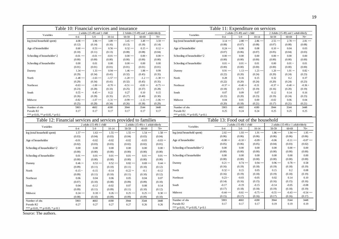
Table 10: Financial services and insurance

Table 11: Expenditure on services

Table 12: Financial services and services provided to families

Table 13: Food out of the household



(0.12) (0.14) (0.16) (0.13) (0.18) (0.14)

Age of householder 0.60 *** 0.53 *** 0.56 *** 0.32 *** 0.15 ** 0.12 **

(0.10) (0.11) (0.13) (0.08) (0.08) (0.04)

Schooling of householder^2 -0.01 *** -0.01 *** -0.01 *** 0.00 *** 0.00 * 0.00 **

(0.00) (0.00) (0.00) (0.00) (0.00) (0.00)

Schooling of householder 0.00 0.01 0.00 0.00 *** 0.00 0.00

(0.01) (0.01) (0.01) (0.01) (0.01) (0.01)

Dummy 1.34 *** 1.33 *** 0.94 *** 1.46 *** 1.88 ** 0.99

(0.29) (0.34) (0.41) (0.32) (0.45) (0.35)

North -1.48 *** -1.63 *** -1.57 *** -1.20 *** -1.2 *** -1.38 ***

(0.29) (0.34) (0.41) (0.32) (0.45) (0.35)

Northeast -0.63 *** -1.00 *** -0.70 ** -0.51 *** -0.81 ** -0.75 ***

(0.23) (0.28) (0.33) (0.25) (0.37) (0.28)

South 0.55 ** 0.45 ** 0.22 0.27 0.10 0.15

(0.26) (0.28) (0.35) (0.27) (0.40) (0.30)

Midwest -0.82 *** -1.07 *** -1.31 *** -0.99 *** -1.15 *** -1.06 ***

(0.25) (0.28) (0.34) (0.26) (0.38) (0.29)

Number of obs 5903 4602 4180 3944 3544 3448

Pseudo R2 0.17 0.17 0.17 0.17 0.17 0.17

*** p<0.01, ** p<0.05, * p<0.1

60-69 70+Variables

2 adults (15-49) and 1 child 2 Adults (15-49) and 1 adult/elderly

0-4 5-9 10-14 50-59


(0.08) (0.07) (0.08) (0.07) (0.08) (0.08)

Age of householder 0.24 *** 0.06 0.08 0.10 ** 0.04 0.03

(0.07) (0.06) (0.07) (0.05) (0.04) (0.03)

Schooling of householder^2 0.00 *** 0.00 0.00 0.00 ** 0.00 0.00

(0.00) (0.00) (0.00) (0.00) (0.00) (0.00)

Schooling of householder 0.01 ** 0.01 ** 0.01 0.00 0.01 * 0.01

(0.00) (0.00) (0.00) (0.00) (0.00) (0.00)

Dummy 0.91 *** 1.13 *** 1.23 *** 1.20 *** 1.01 ** 0.82 *

(0.22) (0.20) (0.24) (0.20) (0.24) (0.23)

North 0.28 0.16 0.15 0.32 0.2 0.37

(0.22) (0.20) (0.24) (0.20) (0.24) (0.23)

Northeast -0.37 ** -0.40 ** -0.31 -0.37 ** -0.40 ** -0.36 *

(0.18) (0.17) (0.19) (0.16) (0.20) (0.19)

South 0.07 0.09 0.07 0.12 0.14 0.16

(0.22) (0.20) (0.23) (0.19) (0.24) (0.23)

Midwest 0.04 0.01 0.00 -0.02 0.06 0.04

(0.20) (0.18) (0.21) (0.17) (0.21) (0.21)

Number of obs 5903 4602 4180 3944 3544 3448

Pseudo R2 0.25 0.24 0.24 0.25 0.25 0.25

*** p<0.01, ** p<0.05, * p<0.1

Variables2 adults (15-49) and 1 child 2 Adults (15-49) and 1 adult/elderly

0-4 5-9 10-14 50-59 60-69 70+


(0.03) (0.04) (0.03) (0.04) (0.03) (0.04)

Age of householder -0.01 -0.02 -0.02 -0.02 -0.03 -0.03 **

(0.02) (0.03) (0.03) (0.02) (0.02) (0.01)

Schooling of householder^2 0.00 0.00 0.00 0.00 0.00 0.00 *

(0.00) (0.00) (0.00) (0.00) (0.00) (0.00)


(0.00) (0.00) (0.00) (0.00) (0.00) (0.00)

Dummy 0.46 ** 0.53 *** 0.52 *** 0.82 *** 0.69 *** 0.44 **

(0.09) (0.11) (0.10) (0.11) (0.10) (0.12)

North -0.15 * -0.15 -0.14 -0.22 ** -0.1 -0.12

(0.09) (0.11) (0.10) (0.11) (0.10) (0.12)

Northeast 0.06 0.04 0.06 0.05 0.04 0.07

(0.07) (0.10) (0.08) (0.09) (0.09) (0.10)

South 0.04 -0.12 -0.02 0.07 0.08 0.14

(0.09) (0.11) (0.09) (0.11) (0.10) (0.12)

Midwest 0.24 *** 0.18 ** 0.26 *** 0.25 *** 0.25 *** 0.30 ***

(0.08) (0.10) (0.09) (0.09) (0.09) (0.10)

Number of obs 5903 4602 4180 3944 3544 3448

Pseudo R2 0.27 0.27 0.27 0.27 0.26 0.26

*** p<0.01, ** p<0.05, * p<0.1

Variables2 adults (15-49) 1 child 2 adults (15-49) e 1 adult/elderly

0-4 5-9 10-14 50-59 60-69 70+


(0.06) (0.06) (0.06) (0.06) (0.06) (0.06)

Age of householder -0.08 ** -0.10 * -0.09 * -0.06 -0.11 *** -0.07 ***

(0.05) (0.06) (0.05) (0.04) (0.03) (0.02)

Schooling of householder^2 0.00 0.00 0.00 0.00 0.00 ** 0.00

(0.00) (0.00) (0.00) (0.00) (0.00) (0.00)


(0.00) (0.00) (0.00) (0.00) (0.00) (0.00)

Dummy 0.21 ** 0.74 *** 0.94 *** 0.96 *** 0.78 ** 0.58

(0.16) (0.19) (0.18) (0.19) (0.18) (0.19)

North 0.32 ** 0.15 0.05 0.15 0.2 0.08

(0.16) (0.19) (0.18) (0.19) (0.18) (0.19)

Northeast 0.23 * -0.03 -0.05 0.02 0.14 0.10

(0.14) (0.16) (0.15) (0.16) (0.15) (0.16)

South -0.17 -0.19 -0.15 -0.14 -0.05 -0.08

(0.17) (0.18) (0.18) (0.19) (0.18) (0.19)

Midwest -0.44 *** -0.61 *** -0.75 *** -0.55 *** -0.43 *** -0.54 ***

(0.15) (0.17) (0.16) (0.17) (0.16) (0.17)

Number of obs 5903 4602 4180 3944 3544 3448

Pseudo R2 0.17 0.17 0.17 0.19 0.19 0.19

*** p<0.01, ** p<0.05, * p<0.1

Variables2 adults (15-49) 1 child 2 adults (15-49) e 1 adult/elderly

0-4 5-9 10-14 50-59 60-69 70+

Download - Age structure and Household Consumption in Brazil - ANPEC · 1 Age structure and Household Consumption in Brazil Flaviane Souza Santiago1, Mônica Viegas Andrade2, Edson Paulo Domingues3

Top Related