energies
Article
Aerodynamic and Structural Integrated OptimizationDesign of Horizontal-Axis Wind Turbine Blades
Jie Zhu 1,2,*, Xin Cai 2 and Rongrong Gu 2
1 College of Civil Engineering and Architecture, Jiaxing University, Jiaxing 314001, China2 College of Mechanics and Materials, Hohai University, Nanjing 210098, China;
[email protected] (X.C.); [email protected] (R.G.)* Correspondence: [email protected]; Tel.: +86-573-8364-6050
Academic Editor: Frede BlaabjergReceived: 14 December 2015; Accepted: 18 January 2016; Published: 22 January 2016
Abstract: A procedure based on MATLAB combined with ANSYS is presented and utilized forthe aerodynamic and structural integrated optimization design of Horizontal-Axis Wind Turbine(HAWT) blades. Three modules are used for this purpose: an aerodynamic analysis module usingthe Blade Element Momentum (BEM) theory, a structural analysis module employing the FiniteElement Method (FEM) and a multi-objective optimization module utilizing the non-dominatedsorting genetic algorithm. The former two provide a sufficiently accurate solution of the aerodynamicand structural performances of the blade; the latter handles the design variables of the optimizationproblem, namely, the main geometrical shape and structural parameters of the blade, and promotesfunction optimization. The scope of the procedure is to achieve the best trade-off performancesbetween the maximum Annual Energy Production (AEP) and the minimum blade mass undervarious design requirements. To prove the efficiency and reliability of the procedure, a commercial1.5 megawatt (MW) HAWT blade is used as a case study. Compared with the original scheme,the optimization results show great improvements for the overall performance of the blade.
Keywords: integrated optimization design; horizontal axis wind turbine; multi-objectiveoptimization; annual energy production; blade mass
1. Introduction
Blades are regarded as the key components of the Horizontal-Axis Wind Turbine (HAWT) systemand have been paid much attention by most of the leading wind turbine manufacturers to developtheir own blade design. As world wind energy market continuously grows, a number of blademanufacturers have emerged recently, especially in China. However, their independent design andmanufacturing capabilities are weak, and the wind blade market is still dominated by the leading windturbine system manufacturers [1]. Thus, to enter the market successfully and be more competitive,improving the fundamental technology on design and production of multi-megawatt (MW) classblades is indispensable.
The design process of the blades can be divided into two stages: the aerodynamic design andthe structural design [2]. From the perspective of aerodynamic design, aerodynamic loads, powerperformance, aerodynamic efficiency, and Annual Energy Production (AEP) are important, and fromthe perspective of structural design, composite material lay-up, mass, stiffness, buckling stability, andfatigue loads are concerned [3]. A successful blade design should take into account the interactionbetween the two stages and satisfy a wide range of objectives, so the design process is a complexmulti-objective optimization task characterized by numerous trade-off decisions. Nevertheless, inorder to simplify the process, the aerodynamic design and the structural design are separated by the
Energies 2016, 9, 66; doi:10.3390/en9020066 www.mdpi.com/journal/energies
Energies 2016, 9, 66 2 of 18
conventional methods. As of now, most of the research is focused mainly on the optimization of eitheraerodynamic or structural performances, which are unable to get the overall optimal solutions [4–9].Only a limited number of works are concerned with the optimization of both aerodynamic andstructural performances, and the relative procedure for this purpose is scarce.
Grujicic [10] developed a multi-disciplinary design-optimization procedure for the design ofa 5 MW HAWT blade with respect to the attainment of a minimal Cost of Energy (COE), andseveral potential solutions for remedying the performance deficiencies of the blade were obtained.Bottasso [11] described procedures for the multi-disciplinary design optimization of wind turbines.The optimization was performed by a multi-stage process that first alternates between an aerodynamicshape optimization to maximize the AEP and a structural blade optimization to minimize the bladeweight, and then combined the two to yield the final optimum solution. However, the problemsonly take a single objective function into account at each time, thus they can not obtain the trade-offsolutions among conflicted objectives.
Benini [12] described a two-objective optimization method to design stall regulated HAWT blades,the aim was to achieve the trade-off solutions between AEP per square meter of wind park and COE.Wang [13,14] applied a novel multi-objective optimization algorithm for the design of wind turbineblades by employing the minimum blade mass and the maximum power coefficient, the maximumAEP and minimum blade mass as the optimization objectives, respectively. However, the blades aretreated as beam models to calculate the structural performances in the above research, and the materiallayups were not considered.
This paper describes a procedure for the aerodynamic and structural integrated multi-optimizationdesign of HAWT blades to maximize the AEP and minimize the blade mass. The scope is to findthe balance between the design process to obtain the optimum overall performance of the blades,by varying the main aerodynamic parameters (chord, twist, span-wise locations of airfoils, and therotational speed) as well as structural parameters (material layup in the spar cap and the position ofthe shear webs) under various design requirements.
2. Modeling of the Blade
2.1. Finite Element Method (FEM) Model of the Blade
As a starting point for the optimization, an initial definition of the blade aerodynamic andstructural configuration is required. In this paper, a commercial 1.5 MW HAWT blade with a length of37 m and a mass of 6580.4 kg is used for a case study.
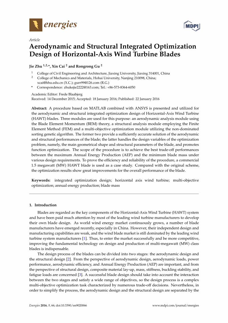
Figure 1 shows the geometry shape of the blade, which can be divided into three areas: root,transition region and aerodynamic region. The root area is normally circular in cross section in orderto match up with the bolted flange, the aerodynamic region uses aerofoil section to capture the wind,and the transition region from the root section to the aerofoil section should be a smooth one forstructural reasons.
Energies 2016, 9, 66 2 of 18
optimization of either aerodynamic or structural performances, which are unable to get the overall
optimal solutions [4–9]. Only a limited number of works are concerned with the optimization of both
aerodynamic and structural performances, and the relative procedure for this purpose is scarce.
Grujicic [10] developed a multi‐disciplinary design‐optimization procedure for the design of a
5 MW HAWT blade with respect to the attainment of a minimal Cost of Energy (COE), and several
potential solutions for remedying the performance deficiencies of the blade were obtained. Bottasso [11]
described procedures for the multi‐disciplinary design optimization of wind turbines. The
optimization was performed by a multi‐stage process that first alternates between an aerodynamic
shape optimization to maximize the AEP and a structural blade optimization to minimize the blade
weight, and then combined the two to yield the final optimum solution. However, the problems
only take a single objective function into account at each time, thus they can not obtain the trade‐off
solutions among conflicted objectives.
Benini [12] described a two‐objective optimization method to design stall regulated HAWT
blades, the aim was to achieve the trade‐off solutions between AEP per square meter of wind park
and COE. Wang [13,14] applied a novel multi‐objective optimization algorithm for the design of
wind turbine blades by employing the minimum blade mass and the maximum power coefficient,
the maximum AEP and minimum blade mass as the optimization objectives, respectively. However,
the blades are treated as beam models to calculate the structural performances in the above research,
and the material layups were not considered.
This paper describes a procedure for the aerodynamic and structural integrated
multi‐optimization design of HAWT blades to maximize the AEP and minimize the blade mass.
The scope is to find the balance between the design process to obtain the optimum overall
performance of the blades, by varying the main aerodynamic parameters (chord, twist, span‐wise
locations of airfoils, and the rotational speed) as well as structural parameters (material layup in the
spar cap and the position of the shear webs) under various design requirements.
2. Modeling of the Blade
2.1. Finite Element Method (FEM) Model of the Blade
As a starting point for the optimization, an initial definition of the blade aerodynamic and
structural configuration is required. In this paper, a commercial 1.5 MW HAWT blade with a length
of 37 m and a mass of 6580.4 kg is used for a case study.
Figure 1 shows the geometry shape of the blade, which can be divided into three areas: root,
transition region and aerodynamic region. The root area is normally circular in cross section in order
to match up with the bolted flange, the aerodynamic region uses aerofoil section to capture the wind,
and the transition region from the root section to the aerofoil section should be a smooth one for
structural reasons.
Figure 1. The geometry shape of the blade.
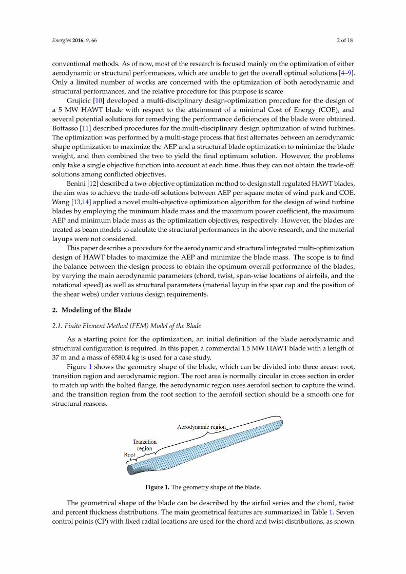
The geometrical shape of the blade can be described by the airfoil series and the chord, twist
and percent thickness distributions. The main geometrical features are summarized in Table 1.
Seven control points (CP) with fixed radial locations are used for the chord and twist distributions,
as shown in Figure 2. The radial locations of the CP3‐7 are defined using half‐cosine spacing, CP1 is
Figure 1. The geometry shape of the blade.
The geometrical shape of the blade can be described by the airfoil series and the chord, twistand percent thickness distributions. The main geometrical features are summarized in Table 1. Sevencontrol points (CP) with fixed radial locations are used for the chord and twist distributions, as shown
Energies 2016, 9, 66 3 of 18
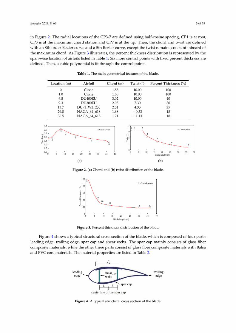
in Figure 2. The radial locations of the CP3-7 are defined using half-cosine spacing, CP1 is at root,CP3 is at the maximum chord station and CP7 is at the tip. Then, the chord and twist are definedwith an 8th order Bezier curve and a 5th Bezier curve, except the twist remains constant inboard ofthe maximum chord. As Figure 3 illustrates, the percent thickness distribution is represented by thespan-wise location of airfoils listed in Table 1. Six more control points with fixed percent thickness aredefined. Then, a cubic polynomial is fit through the control points.
Table 1. The main geometrical features of the blade.
Location (m) Airfoil Chord (m) Twist (˝) Percent Thickness (%)
0 Circle 1.88 10.00 1001.0 Circle 1.88 10.00 1006.8 DU400EU 3.02 10.00 409.3 DU300EU 2.98 7.30 30
13.7 DU91_W2_250 2.51 4.35 2529.8 NACA_64_618 1.68 ´0.33 1836.5 NACA_64_618 1.21 ´1.13 18
Energies 2016, 9, 66 3 of 18
at root, CP3 is at the maximum chord station and CP7 is at the tip. Then, the chord and twist are
defined with an 8th order Bezier curve and a 5th Bezier curve, except the twist remains constant
inboard of the maximum chord. As Figure 3 illustrates, the percent thickness distribution is
represented by the span‐wise location of airfoils listed in Table 1. Six more control points with fixed
percent thickness are defined. Then, a cubic polynomial is fit through the control points.
Table 1. The main geometrical features of the blade.
Location (m) Airfoil Chord (m) Twist (°) Percent Thickness (%)
0 Circle 1.88 10.00 100
1.0 Circle 1.88 10.00 100
6.8 DU400EU 3.02 10.00 40
9.3 DU300EU 2.98 7.30 30
13.7 DU91_W2_250 2.51 4.35 25
29.8 NACA_64_618 1.68 −0.33 18
36.5 NACA_64_618 1.21 −1.13 18
0 5 10 15 20 25 30 35 400.0
0.5
1.0
1.5
2.0
2.5
3.0
3.5
7
Control points
65
43
2
Cho
rd (
m)
1
0 5 10 15 20 25 30 35 40-3
1
5
9
13
76
5
4
321T
wis
t (
)
Blade length (m)
Control points
(a) (b)
Figure 2. (a) Chord and (b) twist distribution of the blade.
0 5 10 15 20 25 30 35 400
20
40
60
80
100
12 1311
10
9
Per
cent
thic
knes
s (%
)
Blade length (m)
Control points8
Figure 3. Percent thickness distribution of the blade.
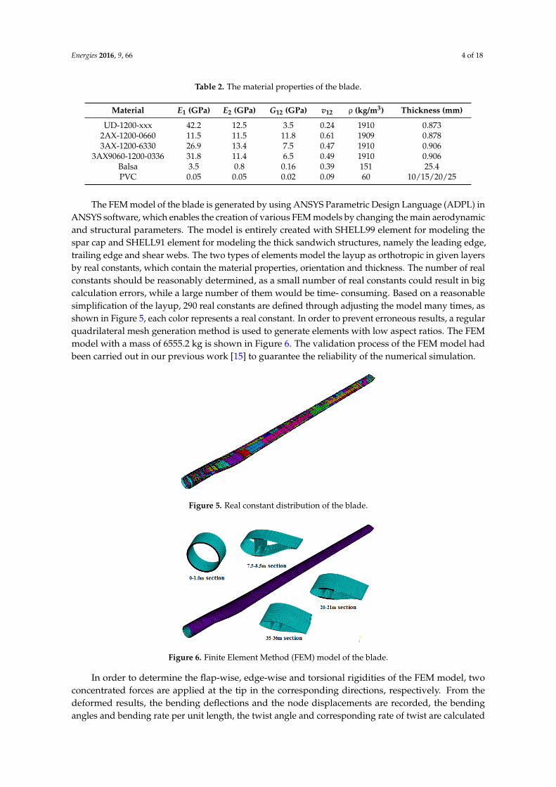
Figure 4 shows a typical structural cross section of the blade, which is composed of four parts:
leading edge, trailing edge, spar cap and shear webs. The spar cap mainly consists of glass fiber
composite materials, while the other three parts consist of glass fiber composite materials with
Balsa and PVC core materials. The material properties are listed in Table 2.
Figure 4. A typical structural cross section of the blade.
Figure 2. (a) Chord and (b) twist distribution of the blade.
Energies 2016, 9, 66 3 of 18
at root, CP3 is at the maximum chord station and CP7 is at the tip. Then, the chord and twist are
defined with an 8th order Bezier curve and a 5th Bezier curve, except the twist remains constant
inboard of the maximum chord. As Figure 3 illustrates, the percent thickness distribution is
represented by the span‐wise location of airfoils listed in Table 1. Six more control points with fixed
percent thickness are defined. Then, a cubic polynomial is fit through the control points.
Table 1. The main geometrical features of the blade.
Location (m) Airfoil Chord (m) Twist (°) Percent Thickness (%)
0 Circle 1.88 10.00 100
1.0 Circle 1.88 10.00 100
6.8 DU400EU 3.02 10.00 40
9.3 DU300EU 2.98 7.30 30
13.7 DU91_W2_250 2.51 4.35 25
29.8 NACA_64_618 1.68 −0.33 18
36.5 NACA_64_618 1.21 −1.13 18
0 5 10 15 20 25 30 35 400.0
0.5
1.0
1.5
2.0
2.5
3.0
3.5
7
Control points
65
43
2
Cho
rd (
m)
1
0 5 10 15 20 25 30 35 40-3
1
5
9
13
76
5
4
321T
wis
t (
)
Blade length (m)
Control points
(a) (b)
Figure 2. (a) Chord and (b) twist distribution of the blade.
0 5 10 15 20 25 30 35 400
20
40
60
80
100
12 1311
10
9
Per
cent
thic
knes
s (%
)
Blade length (m)
Control points8
Figure 3. Percent thickness distribution of the blade.
Figure 4 shows a typical structural cross section of the blade, which is composed of four parts:
leading edge, trailing edge, spar cap and shear webs. The spar cap mainly consists of glass fiber
composite materials, while the other three parts consist of glass fiber composite materials with
Balsa and PVC core materials. The material properties are listed in Table 2.
Figure 4. A typical structural cross section of the blade.
Figure 3. Percent thickness distribution of the blade.
Figure 4 shows a typical structural cross section of the blade, which is composed of four parts:leading edge, trailing edge, spar cap and shear webs. The spar cap mainly consists of glass fibercomposite materials, while the other three parts consist of glass fiber composite materials with Balsaand PVC core materials. The material properties are listed in Table 2.
Energies 2016, 9, 66 3 of 18
at root, CP3 is at the maximum chord station and CP7 is at the tip. Then, the chord and twist are
defined with an 8th order Bezier curve and a 5th Bezier curve, except the twist remains constant
inboard of the maximum chord. As Figure 3 illustrates, the percent thickness distribution is
represented by the span‐wise location of airfoils listed in Table 1. Six more control points with fixed
percent thickness are defined. Then, a cubic polynomial is fit through the control points.
Table 1. The main geometrical features of the blade.
Location (m) Airfoil Chord (m) Twist (°) Percent Thickness (%)
0 Circle 1.88 10.00 100
1.0 Circle 1.88 10.00 100
6.8 DU400EU 3.02 10.00 40
9.3 DU300EU 2.98 7.30 30
13.7 DU91_W2_250 2.51 4.35 25
29.8 NACA_64_618 1.68 −0.33 18
36.5 NACA_64_618 1.21 −1.13 18
0 5 10 15 20 25 30 35 400.0
0.5
1.0
1.5
2.0
2.5
3.0
3.5
7
Control points
65
43
2
Cho
rd (
m)
1
0 5 10 15 20 25 30 35 40-3
1
5
9
13
76
5
4
321
Tw
ist
()
Blade length (m)
Control points
(a) (b)
Figure 2. (a) Chord and (b) twist distribution of the blade.
0 5 10 15 20 25 30 35 400
20
40
60
80
100
12 1311
10
9
Per
cent
thic
knes
s (%
)
Blade length (m)
Control points8
Figure 3. Percent thickness distribution of the blade.
Figure 4 shows a typical structural cross section of the blade, which is composed of four parts:
leading edge, trailing edge, spar cap and shear webs. The spar cap mainly consists of glass fiber
composite materials, while the other three parts consist of glass fiber composite materials with
Balsa and PVC core materials. The material properties are listed in Table 2.
Figure 4. A typical structural cross section of the blade. Figure 4. A typical structural cross section of the blade.
Energies 2016, 9, 66 4 of 18
Table 2. The material properties of the blade.
Material E1 (GPa) E2 (GPa) G12 (GPa) v12 ρ (kg/m3) Thickness (mm)
UD-1200-xxx 42.2 12.5 3.5 0.24 1910 0.8732AX-1200-0660 11.5 11.5 11.8 0.61 1909 0.8783AX-1200-6330 26.9 13.4 7.5 0.47 1910 0.906
3AX9060-1200-0336 31.8 11.4 6.5 0.49 1910 0.906Balsa 3.5 0.8 0.16 0.39 151 25.4PVC 0.05 0.05 0.02 0.09 60 10/15/20/25
The FEM model of the blade is generated by using ANSYS Parametric Design Language (ADPL) inANSYS software, which enables the creation of various FEM models by changing the main aerodynamicand structural parameters. The model is entirely created with SHELL99 element for modeling thespar cap and SHELL91 element for modeling the thick sandwich structures, namely the leading edge,trailing edge and shear webs. The two types of elements model the layup as orthotropic in given layersby real constants, which contain the material properties, orientation and thickness. The number of realconstants should be reasonably determined, as a small number of real constants could result in bigcalculation errors, while a large number of them would be time- consuming. Based on a reasonablesimplification of the layup, 290 real constants are defined through adjusting the model many times, asshown in Figure 5, each color represents a real constant. In order to prevent erroneous results, a regularquadrilateral mesh generation method is used to generate elements with low aspect ratios. The FEMmodel with a mass of 6555.2 kg is shown in Figure 6. The validation process of the FEM model hadbeen carried out in our previous work [15] to guarantee the reliability of the numerical simulation.
Energies 2016, 9, 66 4 of 18
Table 2. The material properties of the blade.
Material E1 (GPa) E2 (GPa) G12 (GPa) v12 (kg/m3) Thickness (mm)
UD‐1200‐xxx 42.2 12.5 3.5 0.24 1910 0.873
2AX‐1200‐0660 11.5 11.5 11.8 0.61 1909 0.878
3AX‐1200‐6330 26.9 13.4 7.5 0.47 1910 0.906
3AX9060‐1200‐0336 31.8 11.4 6.5 0.49 1910 0.906
Balsa 3.5 0.8 0.16 0.39 151 25.4
PVC 0.05 0.05 0.02 0.09 60 10/15/20/25
The FEM model of the blade is generated by using ANSYS Parametric Design Language
(ADPL) in ANSYS software, which enables the creation of various FEM models by changing the
main aerodynamic and structural parameters. The model is entirely created with SHELL99 element
for modeling the spar cap and SHELL91 element for modeling the thick sandwich structures,
namely the leading edge, trailing edge and shear webs. The two types of elements model the layup
as orthotropic in given layers by real constants, which contain the material properties, orientation
and thickness. The number of real constants should be reasonably determined, as a small number of
real constants could result in big calculation errors, while a large number of them would be time‐
consuming. Based on a reasonable simplification of the layup, 290 real constants are defined
through adjusting the model many times, as shown in Figure 5, each color represents a real constant.
In order to prevent erroneous results, a regular quadrilateral mesh generation method is used to
generate elements with low aspect ratios. The FEM model with a mass of 6555.2 kg is shown in
Figure 6. The validation process of the FEM model had been carried out in our previous work [15]
to guarantee the reliability of the numerical simulation.
Figure 5. Real constant distribution of the blade.
Figure 6. Finite Element Method (FEM) model of the blade.
In order to determine the flap‐wise, edge‐wise and torsional rigidities of the FEM model,
two concentrated forces are applied at the tip in the corresponding directions, respectively.
From the deformed results, the bending deflections and the node displacements are recorded,
Figure 5. Real constant distribution of the blade.
Energies 2016, 9, 66 4 of 18
Table 2. The material properties of the blade.
Material E1 (GPa) E2 (GPa) G12 (GPa) v12 (kg/m3) Thickness (mm)
UD‐1200‐xxx 42.2 12.5 3.5 0.24 1910 0.873
2AX‐1200‐0660 11.5 11.5 11.8 0.61 1909 0.878
3AX‐1200‐6330 26.9 13.4 7.5 0.47 1910 0.906
3AX9060‐1200‐0336 31.8 11.4 6.5 0.49 1910 0.906
Balsa 3.5 0.8 0.16 0.39 151 25.4
PVC 0.05 0.05 0.02 0.09 60 10/15/20/25
The FEM model of the blade is generated by using ANSYS Parametric Design Language
(ADPL) in ANSYS software, which enables the creation of various FEM models by changing the
main aerodynamic and structural parameters. The model is entirely created with SHELL99 element
for modeling the spar cap and SHELL91 element for modeling the thick sandwich structures,
namely the leading edge, trailing edge and shear webs. The two types of elements model the layup
as orthotropic in given layers by real constants, which contain the material properties, orientation
and thickness. The number of real constants should be reasonably determined, as a small number of
real constants could result in big calculation errors, while a large number of them would be time‐
consuming. Based on a reasonable simplification of the layup, 290 real constants are defined
through adjusting the model many times, as shown in Figure 5, each color represents a real constant.
In order to prevent erroneous results, a regular quadrilateral mesh generation method is used to
generate elements with low aspect ratios. The FEM model with a mass of 6555.2 kg is shown in
Figure 6. The validation process of the FEM model had been carried out in our previous work [15]
to guarantee the reliability of the numerical simulation.
Figure 5. Real constant distribution of the blade.
Figure 6. Finite Element Method (FEM) model of the blade.
In order to determine the flap‐wise, edge‐wise and torsional rigidities of the FEM model,
two concentrated forces are applied at the tip in the corresponding directions, respectively.
From the deformed results, the bending deflections and the node displacements are recorded,
Figure 6. Finite Element Method (FEM) model of the blade.
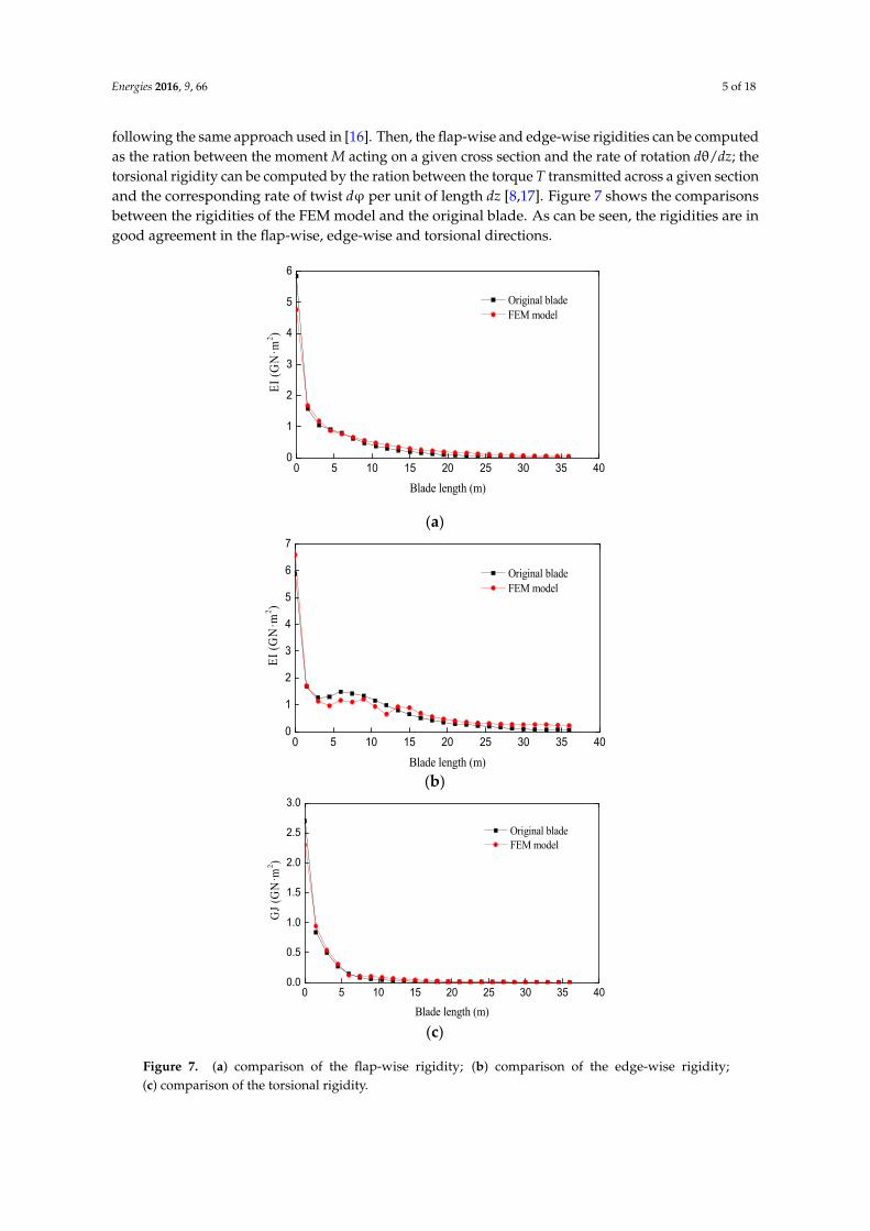
In order to determine the flap-wise, edge-wise and torsional rigidities of the FEM model, twoconcentrated forces are applied at the tip in the corresponding directions, respectively. From thedeformed results, the bending deflections and the node displacements are recorded, the bendingangles and bending rate per unit length, the twist angle and corresponding rate of twist are calculated
Energies 2016, 9, 66 5 of 18
following the same approach used in [16]. Then, the flap-wise and edge-wise rigidities can be computedas the ration between the moment M acting on a given cross section and the rate of rotation dθ/dz; thetorsional rigidity can be computed by the ration between the torque T transmitted across a given sectionand the corresponding rate of twist dϕ per unit of length dz [8,17]. Figure 7 shows the comparisonsbetween the rigidities of the FEM model and the original blade. As can be seen, the rigidities are ingood agreement in the flap-wise, edge-wise and torsional directions.
Energies 2016, 9, 66 5 of 18
the bending angles and bending rate per unit length, the twist angle and corresponding rate of twist
are calculated following the same approach used in [16]. Then, the flap‐wise and edge‐wise
rigidities can be computed as the ration between the moment M acting on a given cross section and
the rate of rotation dθ/dz; the torsional rigidity can be computed by the ration between the torque T
transmitted across a given section and the corresponding rate of twist dφ per unit of length dz [8,17].
Figure 7 shows the comparisons between the rigidities of the FEM model and the original blade.
As can be seen, the rigidities are in good agreement in the flap‐wise, edge‐wise and torsional directions.
0 5 10 15 20 25 30 35 400
1
2
3
4
5
6E
I (G
N·m
2 )
Blade length (m)
Original blade FEM model
(a)
0 5 10 15 20 25 30 35 400
1
2
3
4
5
6
7
Original blade FEM model
EI
(GN
·m2 )
Blade length (m) (b)
0 5 10 15 20 25 30 35 400.0
0.5
1.0
1.5
2.0
2.5
3.0
GJ
(GN
·m2 )
Blade length (m)
Original blade FEM model
(c)
Figure 7. (a) comparison of the flap‐wise rigidity; (b) comparison of the edge‐wise rigidity;
(c) comparison of the torsional rigidity.
2.2. Aerodynamic Loads of the Blade
Aerodynamic loads for design are computed using Blade Element Momentum (BEM)
theory [18,19], which include the operational and the ultimate load cases. The operational load case
considers the wind condition corresponding to the maximum root flap bending moment under
Figure 7. (a) comparison of the flap-wise rigidity; (b) comparison of the edge-wise rigidity;(c) comparison of the torsional rigidity.
Energies 2016, 9, 66 6 of 18
2.2. Aerodynamic Loads of the Blade
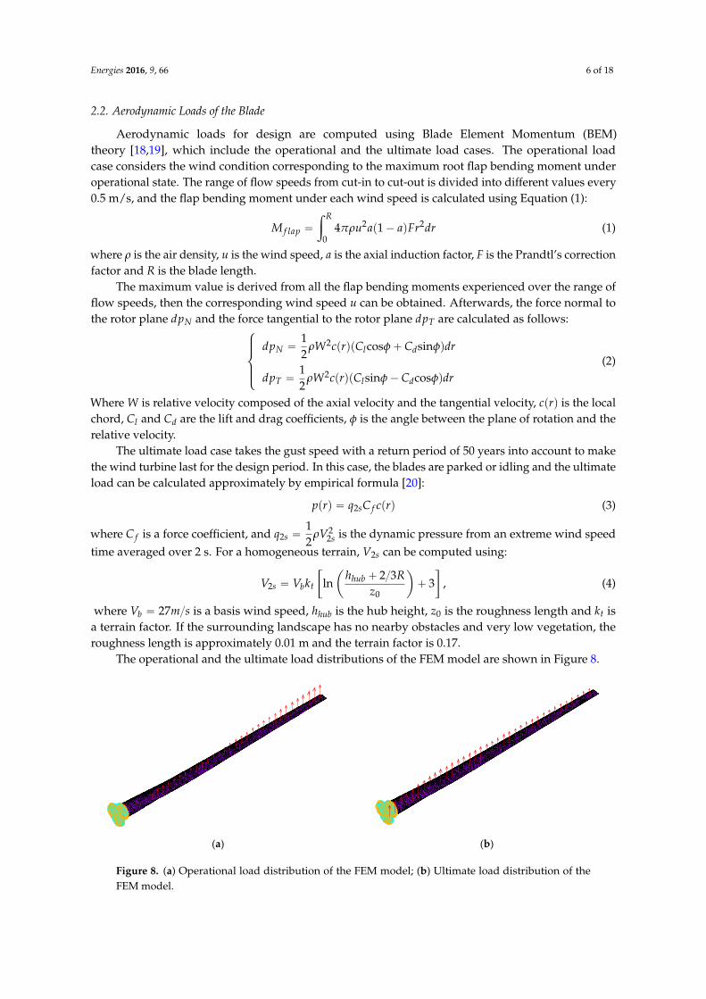
Aerodynamic loads for design are computed using Blade Element Momentum (BEM)theory [18,19], which include the operational and the ultimate load cases. The operational loadcase considers the wind condition corresponding to the maximum root flap bending moment underoperational state. The range of flow speeds from cut-in to cut-out is divided into different values every0.5 m/s, and the flap bending moment under each wind speed is calculated using Equation (1):
M f lap “
ż R
04πρu2ap1´ aqFr2dr (1)
where ρ is the air density, u is the wind speed, a is the axial induction factor, F is the Prandtl’s correctionfactor and R is the blade length.
The maximum value is derived from all the flap bending moments experienced over the range offlow speeds, then the corresponding wind speed u can be obtained. Afterwards, the force normal tothe rotor plane dpN and the force tangential to the rotor plane dpT are calculated as follows:
$
’
’
&
’
’
%
dpN “12
ρW2cprqpClcosφ` Cdsinφqdr
dpT “12
ρW2cprqpClsinφ´ Cdcosφqdr(2)
Where W is relative velocity composed of the axial velocity and the tangential velocity, cprq is the localchord, Cl and Cd are the lift and drag coefficients, φ is the angle between the plane of rotation and therelative velocity.
The ultimate load case takes the gust speed with a return period of 50 years into account to makethe wind turbine last for the design period. In this case, the blades are parked or idling and the ultimateload can be calculated approximately by empirical formula [20]:
pprq “ q2sC f cprq (3)
where C f is a force coefficient, and q2s “12
ρV22s is the dynamic pressure from an extreme wind speed
time averaged over 2 s. For a homogeneous terrain, V2s can be computed using:
V2s “ Vbkt
„
lnˆ
hhub ` 2{3Rz0
˙
` 3
, (4)
where Vb “ 27m{s is a basis wind speed, hhub is the hub height, z0 is the roughness length and kt isa terrain factor. If the surrounding landscape has no nearby obstacles and very low vegetation, theroughness length is approximately 0.01 m and the terrain factor is 0.17.
The operational and the ultimate load distributions of the FEM model are shown in Figure 8.
Energies 2016, 9, 66 6 of 18
operational state. The range of flow speeds from cut‐in to cut‐out is divided into different values
every 0.5 m/s, and the flap bending moment under each wind speed is calculated using Equation (1):
2 2 R
flap 0M 4πρu a ‐ a Fr dr(1 ) (1)
where ρ is the air density, u is the wind speed, a is the axial induction factor, F is the Prandtl’s
correction factor and R is the blade length.
The maximum value is derived from all the flap bending moments experienced over the range of
flow speeds, then the corresponding wind speed u can be obtained. Afterwards, the force normal to
the rotor plane Ndp and the force tangential to the rotor plane Tdp are calculated as follows:
2
2
N l d
T l d
dp ρW c r C cos C sin dr
dp ρW c r C sin C cos dr
1= ( )( )21
= ( )( )2
(2)
Where W is relative velocity composed of the axial velocity and the tangential velocity, c r( ) is the
local chord, Cl and Cd are the lift and drag coefficients, is the angle between the plane of rotation
and the relative velocity.
The ultimate load case takes the gust speed with a return period of 50 years into account to
make the wind turbine last for the design period. In this case, the blades are parked or idling and
the ultimate load can be calculated approximately by empirical formula [20]:
2s fp r q C c r( ) ( ) (3)
where Cf is a force coefficient, and 22s 2sq ρV
1
2 is the dynamic pressure from an extreme wind
speed time averaged over 2 s. For a homogeneous terrain, V2s can be computed using:
hub
2s b t
0
h + RV V k ln +
z
2 33
,
(4)
where bV = m / s27 is a basis wind speed, hubh is the hub height, 0z is the roughness length
and tk is a terrain factor. If the surrounding landscape has no nearby obstacles and very low
vegetation, the roughness length is approximately 0.01 m and the terrain factor is 0.17.
The operational and the ultimate load distributions of the FEM model are shown in Figure 8.
(a) (b)
Figure 8. (a) Operational load distribution of the FEM model; (b) Ultimate load distribution of the
FEM model. Figure 8. (a) Operational load distribution of the FEM model; (b) Ultimate load distribution of theFEM model.
Energies 2016, 9, 66 7 of 18
3. Formulation of the Optimization Problem
3.1. The Objective Functions
A successful blade design must satisfy a wide range of objectives, such as maximization of theAEP and power coefficient, resistance to extreme and fatigue loads, restriction of tip deflections,avoiding resonances, and minimization of weight and cost, some of these objectives are in conflict [2].In order to make wind energy more competitive with other energy sources, manufacturers areconcentrating on increasing the energy output capacity and bringing down the cost of blades andother components at the same time, so minimizing the COE is an attractive target pursued by manyresearchers. However, the cost of the blades involves many factors such as cost of the materials,production tooling, manufacturing labor and overland transportation, and some of them are hardto estimate. According to some studies [21,22], reducing materials to minimize the blade mass cannot only cause cost reduction of the blade but also have a multiplier effect through out the systemincluding the foundation. Thus, the maximum AEP and the minimum blade mass are taken as theobjective functions.
The energy that can be captured by a wind turbine depends upon the power versus wind speedcharacteristic of the turbine and the wind-speed distribution at the turbine site. The wind-speeddistribution is represented by the Weibull function. The AEP is defined as in Equations (5)–(7):
f p1q “ AEP “Nÿ
i“1
12rPpuiq ` Ppui`1qs¨ f pui ă u0 ă ui`1q ˆ 8760 (5)
Ppuiq “
ż R
04πr3ρuiω
2a1p1´ aqFdr (6)
f pui ă u0 ă ui`1q “ expˆ
´
´uiA
¯k˙
´ expˆ
´
´ui`1
A
¯k˙
, (7)
where Ppuiq is the power under wind speed ui, f pui ă u0 ă ui`1q is the probability that the windspeed lies between ui and ui` 1, ω is the rotational speed of the blade, a1 is the tangential inductionfactor, k is a form factor and A is a scaling factor.
The blade mass depends upon the consumption of materials, which can be expressed as:
f p2q “ mass “ÿ
i
ρi ˆVi (8)
where ρi is the material density, Vi is the volume of the material.
3.2. Design Variables
The geometrical shape and the rotational speed of the blade contribute directly to the aerodynamicperformances. Therefore, the values of the control points in Figures 2 and 3 and the rotational speed areselected as aerodynamic design variables, while the blade length and the airfoil series are employedas the basic parameters. In order to match up with the bolted flange conveniently, the root diameterremains unchanged, which means the chord value of CP1 is fixed. Moreover, the chord of CP2 is equalto CP1, so the chord values of CP3-7 are defined as five aerodynamic variables (x1 to x5). As the twistremains constant inboard of the maximum chord, which means the twists of CP1-3 are the same, thenthe twist values of CP3-7 are defined as another five aerodynamic variables (x6 to x10). The span-wiselocations of CP8 and CP13 are also fixed, one is at root and the other is at tip, thus the locationsof CP9-12 (airfoils with relative thickness of 40%, 30%, 25% and 18%) are employed as four moreaerodynamic variables (x11 to x14). In addition, the rated rotational speed of the rotor is selected as thelast aerodynamic variable (x15).
The spar cap of the blade is primarily designed with a relatively large thickness to carry theaerodynamic loads, so it makes a major contribution to the blade mass [23]. In addition, the blademass can further decrease by positioning the shear webs appropriately. Therefore, the number and
Energies 2016, 9, 66 8 of 18
location of layers in the spar cap, the width of the spar cap, and the position of the shear webs areselected as the structural design variables.
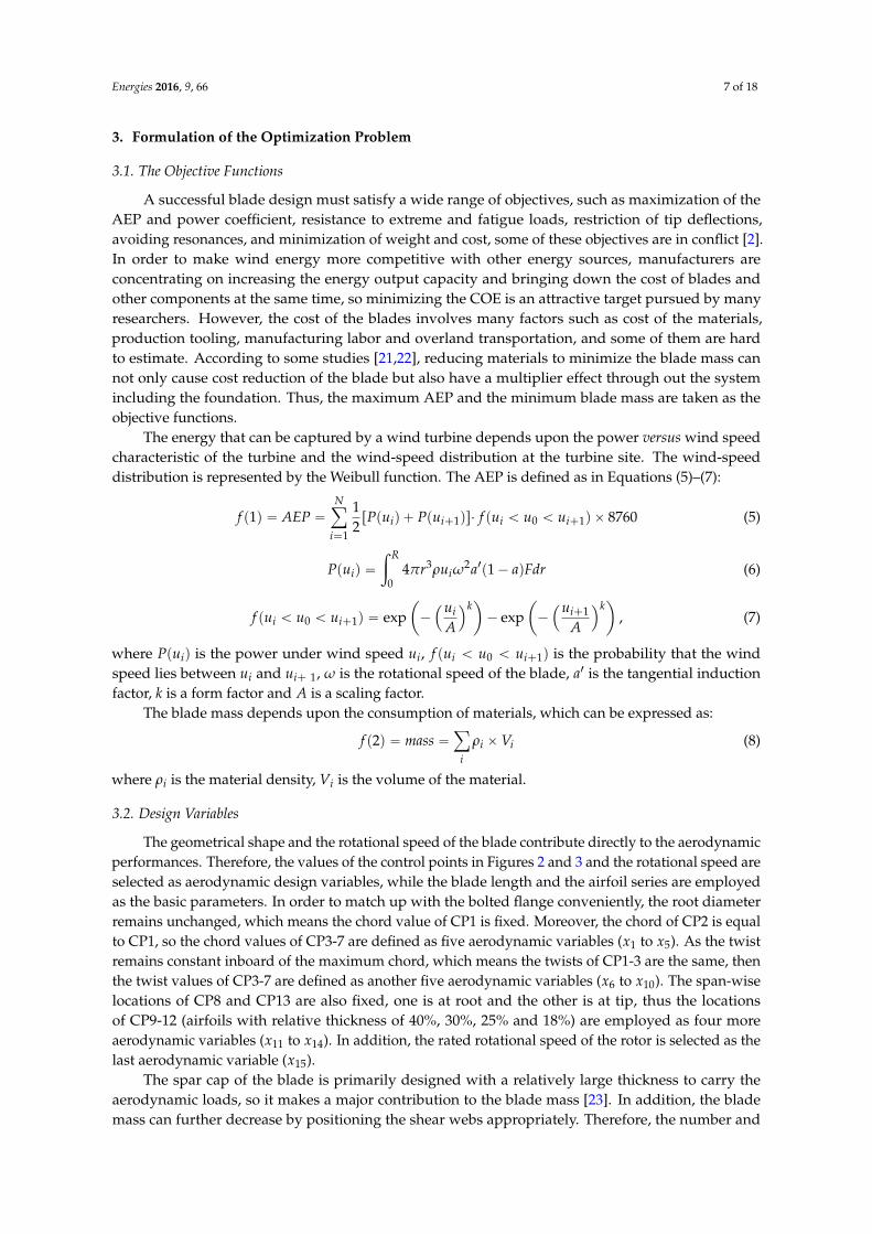
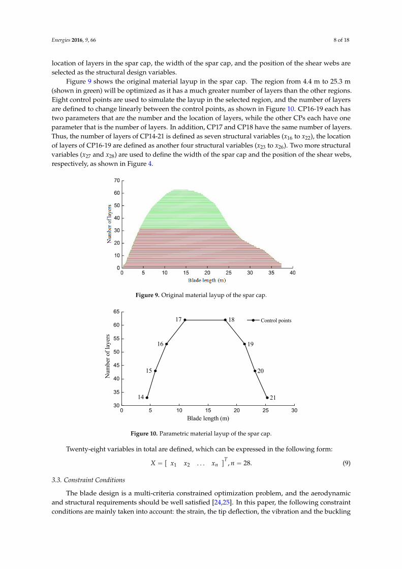
Figure 9 shows the original material layup in the spar cap. The region from 4.4 m to 25.3 m(shown in green) will be optimized as it has a much greater number of layers than the other regions.Eight control points are used to simulate the layup in the selected region, and the number of layersare defined to change linearly between the control points, as shown in Figure 10. CP16-19 each hastwo parameters that are the number and the location of layers, while the other CPs each have oneparameter that is the number of layers. In addition, CP17 and CP18 have the same number of layers.Thus, the number of layers of CP14-21 is defined as seven structural variables (x16 to x22), the locationof layers of CP16-19 are defined as another four structural variables (x23 to x26). Two more structuralvariables (x27 and x28) are used to define the width of the spar cap and the position of the shear webs,respectively, as shown in Figure 4.
Energies 2016, 9, 66 8 of 18
40%, 30%, 25% and 18%) are employed as four more aerodynamic variables ( 11x to 14x ).
In addition, the rated rotational speed of the rotor is selected as the last aerodynamic variable ( 15x ).
The spar cap of the blade is primarily designed with a relatively large thickness to carry the
aerodynamic loads, so it makes a major contribution to the blade mass [23]. In addition, the blade
mass can further decrease by positioning the shear webs appropriately. Therefore, the number and
location of layers in the spar cap, the width of the spar cap, and the position of the shear webs are
selected as the structural design variables.
Figure 9 shows the original material layup in the spar cap. The region from 4.4 m to 25.3 m
(shown in green) will be optimized as it has a much greater number of layers than the other regions.
Eight control points are used to simulate the layup in the selected region, and the number of layers
are defined to change linearly between the control points, as shown in Figure 10. CP16‐19 each has
two parameters that are the number and the location of layers, while the other CPs each have one
parameter that is the number of layers. In addition, CP17 and CP18 have the same number of layers.
Thus, the number of layers of CP14‐21 is defined as seven structural variables (x16 to x22), the
location of layers of CP16‐19 are defined as another four structural variables (x23 to x26). Two more
structural variables (x27 and x28) are used to define the width of the spar cap and the position of the
shear webs, respectively, as shown in Figure 4.
Figure 9. Original material layup of the spar cap.
0 5 10 15 20 25 3030
35
40
45
50
55
60
65
21
20
19
1817
16
15
Num
ber
of la
yers
Blade length (m)
Control points
14
Figure 10. Parametric material layup of the spar cap.
Twenty‐eight variables in total are defined, which can be expressed in the following form:
T1 2 nX x x x ,n =[ ] 28
. (9)
3.3. Constraint Conditions
The blade design is a multi‐criteria constrained optimization problem, and the aerodynamic
and structural requirements should be well satisfied [24,25]. In this paper, the following constraint
Figure 9. Original material layup of the spar cap.
Energies 2016, 9, 66 8 of 18
40%, 30%, 25% and 18%) are employed as four more aerodynamic variables ( 11x to 14x ).
In addition, the rated rotational speed of the rotor is selected as the last aerodynamic variable ( 15x ).
The spar cap of the blade is primarily designed with a relatively large thickness to carry the
aerodynamic loads, so it makes a major contribution to the blade mass [23]. In addition, the blade
mass can further decrease by positioning the shear webs appropriately. Therefore, the number and
location of layers in the spar cap, the width of the spar cap, and the position of the shear webs are
selected as the structural design variables.
Figure 9 shows the original material layup in the spar cap. The region from 4.4 m to 25.3 m
(shown in green) will be optimized as it has a much greater number of layers than the other regions.
Eight control points are used to simulate the layup in the selected region, and the number of layers
are defined to change linearly between the control points, as shown in Figure 10. CP16‐19 each has
two parameters that are the number and the location of layers, while the other CPs each have one
parameter that is the number of layers. In addition, CP17 and CP18 have the same number of layers.
Thus, the number of layers of CP14‐21 is defined as seven structural variables (x16 to x22), the
location of layers of CP16‐19 are defined as another four structural variables (x23 to x26). Two more
structural variables (x27 and x28) are used to define the width of the spar cap and the position of the
shear webs, respectively, as shown in Figure 4.
Figure 9. Original material layup of the spar cap.
0 5 10 15 20 25 3030
35
40
45
50
55
60
65
21
20
19
1817
16
15
Num
ber
of la
yers
Blade length (m)
Control points
14
Figure 10. Parametric material layup of the spar cap.
Twenty‐eight variables in total are defined, which can be expressed in the following form:
T1 2 nX x x x ,n =[ ] 28
. (9)
3.3. Constraint Conditions
The blade design is a multi‐criteria constrained optimization problem, and the aerodynamic
and structural requirements should be well satisfied [24,25]. In this paper, the following constraint
Figure 10. Parametric material layup of the spar cap.
Twenty-eight variables in total are defined, which can be expressed in the following form:
X “ r x1 x2 . . . xn sT
, n “ 28. (9)
3.3. Constraint Conditions
The blade design is a multi-criteria constrained optimization problem, and the aerodynamicand structural requirements should be well satisfied [24,25]. In this paper, the following constraintconditions are mainly taken into account: the strain, the tip deflection, the vibration and the buckling
Energies 2016, 9, 66 9 of 18
constraints. These constraints represent the strength, stiffness, dynamic behavior, and stability designrequirements, respectively.
(1) Generally, the stress and the strain criterions should be considered to reflect the strength ofthe blade. However, the maximum stress generated in the considered 1.5 MW blade under differentloads is far less than the allowable stress, while the maximum strain is much closer to the design value.Therefore, only the strain criterion is used to verify that no elements in the model exceeded the designstrains of the material [22]. This is expressed as follows:
εmax ď εd{γS1, (10)
where εmax is the maximum equivalent strain, εd is the permissible strain, and γs1 is the strainsafety factor.
(2) In order to prevent the collision between the blade tip and the tower, the maximum tipdeflection should be less than the set value. This can be expressed as follows:
dmax ď dd{γS2, (11)
where dmax is the maximum tip deflection, dd is the allowable tip deflection, and γs2 is the tip deflectionsafety factor.
(3) In order to avoid resonance, the natural frequency of the blade should be separated from theharmonic vibration associated with rotor rotation. This is expressed in the inequality form:
|Fblade´1 ´ 3Frotor| ě ∆, (12)
where Fblade´1 is the first natural frequency of the blade, Frotor is the frequency of the rotor rotation,and ∆ is the associated allowable tolerance.
(4) Since the blade is a thin-walled structure, its surface panels near the root are particularlyvulnerable to elastic instability, and the buckling problem must be addressed [23]. In order to avoidbuckling failure, the buckling load should be greater than ultimate loads. This can be expressedas follows:
λ1 ě 1.0ˆ γS3, (13)
where λ1 is a ratio of the buckling load to the maximum ultimate load, called lowest bucklingeigenvalue, and γs3 is the buckling safety factor.
In addition, the lower and upper bounds of design variables should be set appropriately to controlthe change range, shown in Equation (14a). The twist, chord, and relative thickness distributionsare all required to be monotonically decreasing, so the corresponding variables should be satisfiedwith the inequality form in Equation (14b,c). Considering the manufacturing maneuverability andthe continuity of the material layup, the variables that represent the number of layers are requiredto be monotonically increasing to a maximum value and then monotonically decreasing, shown inEquation (14d,e).
$
’
’
’
’
’
’
’
’
’
&
’
’
’
’
’
’
’
’
’
%
xLi ď xi ď xU
i i “ 1, 2, ..., 28 paq
xj ´ xj`1 ą 0 j “ 1, 2, 3, 4, 6, 7, 8, 9 pbq
xk ´ xk`1 ă 0 j “ 11, 12, 13 pcq
xg ´ xg`1 ď 0 g “ 16, 17, 18 pdq
xh ´ xh`1 ě 0 h “ 19, 20, 21 peq
, (14)
where xL is the lower bound of the variables, and xU is the upper bound of the variables.The lower and upper bounds of the variables and the constraint conditions are shown in Table 3.
Energies 2016, 9, 66 10 of 18
Table 3. Lower and upper bounds of the variables and the constraint conditions.
Parameter Lower Bound Upper Bound Unit
x1-x5 1.0 3.3 mx6-x10 ´2.0 12.0 ˝
x11-x14 6.0 30.0 mx15 10 25 rpmx16 28 38 -x17 28 48 -x18 33 58 -x19 35 65 -x20 33 55 -x21 28 45 -x22 28 40 -x23 7.0 9.0 mx24 10.0 13.0 m
x25 16.0 19.0 mx26 20.5 22.0 mx27 0.13 0.25 mx28 0.50 0.70 m
εmax - 0.005 -dmax - 5.5 mλ1 1.2 - -
Fblade´1 ď3Frotor ´ 0.3 or ě3Frotor + 0.3 Hz
4. The Integrated Optimization Design Procedure
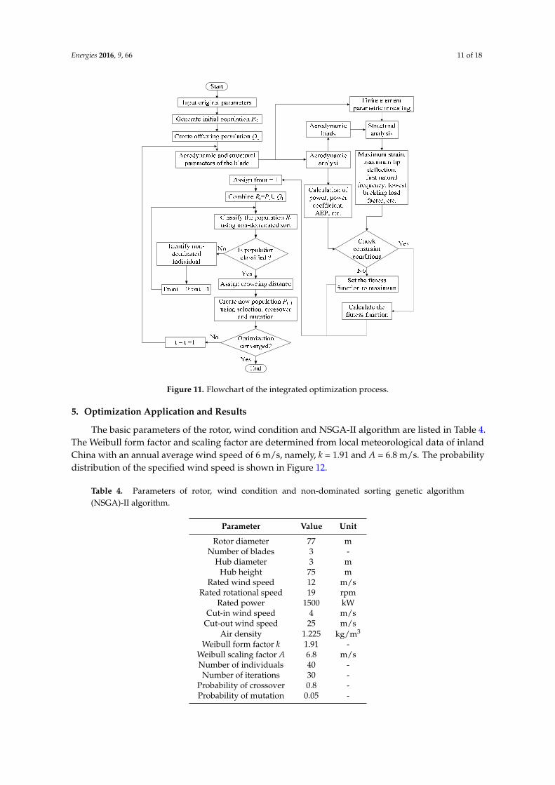
The purpose of the present work is to improve the overall performance of HAWT blades by meansof an optimization of its aerodynamic and structural integrated design, a procedure that interfacesboth the MATLAB optimization tool and develops the finite element software ANSYS. Three modulesare used in the procedure: an aerodynamic analysis module, a structural analysis module and amulti-objective optimization module. The former two provide a sufficiently accurate solution ofthe aerodynamic performances and structural behaviors of the blade; the latter handles the designvariables of the optimization problem and promotes functions optimization. The non-dominatedsorting genetic algorithm (NSGA) II [26–28] is adapted for the integrated optimization design. It is oneof the most efficient and well-known multi-objective evolutionary algorithms and has been widelyapplied to solve complicated optimization problems. According to the method, the Pareto optimalfront can be obtained considering the set of Non-Dominated Solutions.
Figure 11 shows the flowchart of the integrated optimization process. After inputting the originalparameters, an initial population is generated randomly in MATLAB with the aerodynamic andstructural variables written in a string of genes. The aerodynamic variables are used to define thegeometry shape of the blade while the structural variables are used to define the internal structure.Then, the BEM theory is applied to evaluate the aerodynamic performance, such as power, powercoefficient, aerodynamic loads, etc. Meanwhile, a macro file that can transfer the variables fromMATLAB into ANSYS is created using APDL language. Through some specific commands, theprocedure opens the software ANSYS, calls the macro file to generate a parametric FEM model ofthe blade and simulates the load cases in order to obtain the structural behaviors, namely, the strainlevel, the tip deflection, the natural frequencies, the bulking load factors, etc. After several constraintconditions have been checked, two appropriate fitness functions are evaluated. The next step is toclassify the solutions according to a fast non-dominated sorting approach and assign the crowdingdistance. Finally, a new population is created and the process can restart until the optimizationprocedure converges.
Energies 2016, 9, 66 11 of 18Energies 2016, 9, 66 11 of 18
Figure 11. Flowchart of the integrated optimization process.
5. Optimization Application and Results
The basic parameters of the rotor, wind condition and NSGA‐II algorithm are listed in Table 4.
The Weibull form factor and scaling factor are determined from local meteorological data of inland
China with an annual average wind speed of 6 m/s, namely, k = 1.91 and A = 6.8 m/s.
The probability distribution of the specified wind speed is shown in Figure 12.
Table 4. Parameters of rotor, wind condition and non‐dominated sorting genetic algorithm
(NSGA)‐II algorithm.
Parameter Value Unit
Rotor diameter 77 m
Number of blades 3 ‐
Hub diameter 3 m
Hub height 75 m
Rated wind speed 12 m/s
Rated rotational speed 19 rpm
Rated power 1500 kW
Cut‐in wind speed 4 m/s
Cut‐out wind speed 25 m/s
Air density 1.225 kg/m3
Weibull form factor k 1.91 ‐
Weibull scaling factor A 6.8 m/s
Number of individuals 40 ‐
Number of iterations 30 ‐
Probability of crossover 0.8 ‐
Probability of mutation 0.05 ‐
Figure 11. Flowchart of the integrated optimization process.
5. Optimization Application and Results
The basic parameters of the rotor, wind condition and NSGA-II algorithm are listed in Table 4.The Weibull form factor and scaling factor are determined from local meteorological data of inlandChina with an annual average wind speed of 6 m/s, namely, k = 1.91 and A = 6.8 m/s. The probabilitydistribution of the specified wind speed is shown in Figure 12.
Table 4. Parameters of rotor, wind condition and non-dominated sorting genetic algorithm(NSGA)-II algorithm.
Parameter Value Unit
Rotor diameter 77 mNumber of blades 3 -
Hub diameter 3 mHub height 75 m
Rated wind speed 12 m/sRated rotational speed 19 rpm
Rated power 1500 kWCut-in wind speed 4 m/s
Cut-out wind speed 25 m/sAir density 1.225 kg/m3
Weibull form factor k 1.91 -Weibull scaling factor A 6.8 m/sNumber of individuals 40 -Number of iterations 30 -
Probability of crossover 0.8 -Probability of mutation 0.05 -
Energies 2016, 9, 66 12 of 18Energies 2016, 9, 66 12 of 18
0 5 10 15 20 25-0.02
0.00
0.02
0.04
0.06
0.08
0.10
0.12
0.14
Pro
babi
lity
Wind speed (m/s)
k=1.91 c=6.8 Weibull distribution
Figure 12. Weibull probability distribution of wind speed.
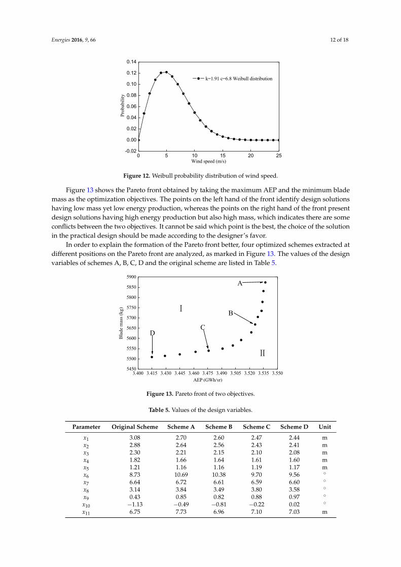
Figure 13 shows the Pareto front obtained by taking the maximum AEP and the minimum
blade mass as the optimization objectives. The points on the left hand of the front identify design
solutions having low mass yet low energy production, whereas the points on the right hand of the
front present design solutions having high energy production but also high mass, which indicates
there are some conflicts between the two objectives. It cannot be said which point is the best, the
choice of the solution in the practical design should be made according to the designer’s favor.
In order to explain the formation of the Pareto front better, four optimized schemes extracted
at different positions on the Pareto front are analyzed, as marked in Figure 13. The values of the
design variables of schemes A, B, C, D and the original scheme are listed in Table 5.
3.400 3.415 3.430 3.445 3.460 3.475 3.490 3.505 3.520 3.535 3.5505450
5500
5550
5600
5650
5700
5750
5800
5850
5900
Ⅰ
Ⅱ
DC
B
A
Bla
de m
ass
(kg)
AEP (GWh/yr)
Figure 13. Pareto front of two objectives.
Table 5. Values of the design variables.
Parameter Original Scheme Scheme A Scheme B Scheme C Scheme D Unit
x1 3.08 2.70 2.60 2.47 2.44 m
x2 2.88 2.64 2.56 2.43 2.41 m
x3 2.30 2.21 2.15 2.10 2.08 m
x4 1.82 1.66 1.64 1.61 1.60 m
x5 1.21 1.16 1.16 1.19 1.17 m
x6 8.73 10.69 10.38 9.70 9.56 °
x7 6.64 6.72 6.61 6.59 6.60 °
x8 3.14 3.84 3.49 3.80 3.58 °
x9 0.43 0.85 0.82 0.88 0.97 °
x10 −1.13 −0.49 −0.81 −0.22 0.02 °
x11 6.75 7.73 6.96 7.10 7.03 m
Figure 12. Weibull probability distribution of wind speed.
Figure 13 shows the Pareto front obtained by taking the maximum AEP and the minimum blademass as the optimization objectives. The points on the left hand of the front identify design solutionshaving low mass yet low energy production, whereas the points on the right hand of the front presentdesign solutions having high energy production but also high mass, which indicates there are someconflicts between the two objectives. It cannot be said which point is the best, the choice of the solutionin the practical design should be made according to the designer’s favor.
In order to explain the formation of the Pareto front better, four optimized schemes extracted atdifferent positions on the Pareto front are analyzed, as marked in Figure 13. The values of the designvariables of schemes A, B, C, D and the original scheme are listed in Table 5.
Energies 2016, 9, 66 12 of 18
0 5 10 15 20 25-0.02
0.00
0.02
0.04
0.06
0.08
0.10
0.12
0.14
Pro
babi
lity
Wind speed (m/s)
k=1.91 c=6.8 Weibull distribution
Figure 12. Weibull probability distribution of wind speed.
Figure 13 shows the Pareto front obtained by taking the maximum AEP and the minimum
blade mass as the optimization objectives. The points on the left hand of the front identify design
solutions having low mass yet low energy production, whereas the points on the right hand of the
front present design solutions having high energy production but also high mass, which indicates
there are some conflicts between the two objectives. It cannot be said which point is the best, the
choice of the solution in the practical design should be made according to the designer’s favor.
In order to explain the formation of the Pareto front better, four optimized schemes extracted
at different positions on the Pareto front are analyzed, as marked in Figure 13. The values of the
design variables of schemes A, B, C, D and the original scheme are listed in Table 5.
3.400 3.415 3.430 3.445 3.460 3.475 3.490 3.505 3.520 3.535 3.5505450
5500
5550
5600
5650
5700
5750
5800
5850
5900
Ⅰ
Ⅱ
DC
B
A
Bla
de m
ass
(kg)
AEP (GWh/yr)
Figure 13. Pareto front of two objectives.
Table 5. Values of the design variables.
Parameter Original Scheme Scheme A Scheme B Scheme C Scheme D Unit
x1 3.08 2.70 2.60 2.47 2.44 m
x2 2.88 2.64 2.56 2.43 2.41 m
x3 2.30 2.21 2.15 2.10 2.08 m
x4 1.82 1.66 1.64 1.61 1.60 m
x5 1.21 1.16 1.16 1.19 1.17 m
x6 8.73 10.69 10.38 9.70 9.56 °
x7 6.64 6.72 6.61 6.59 6.60 °
x8 3.14 3.84 3.49 3.80 3.58 °
x9 0.43 0.85 0.82 0.88 0.97 °
x10 −1.13 −0.49 −0.81 −0.22 0.02 °
x11 6.75 7.73 6.96 7.10 7.03 m
Figure 13. Pareto front of two objectives.
Table 5. Values of the design variables.
Parameter Original Scheme Scheme A Scheme B Scheme C Scheme D Unit
x1 3.08 2.70 2.60 2.47 2.44 mx2 2.88 2.64 2.56 2.43 2.41 mx3 2.30 2.21 2.15 2.10 2.08 mx4 1.82 1.66 1.64 1.61 1.60 mx5 1.21 1.16 1.16 1.19 1.17 mx6 8.73 10.69 10.38 9.70 9.56 ˝
x7 6.64 6.72 6.61 6.59 6.60 ˝
x8 3.14 3.84 3.49 3.80 3.58 ˝
x9 0.43 0.85 0.82 0.88 0.97 ˝
x10 ´1.13 ´0.49 ´0.81 ´0.22 0.02 ˝
x11 6.75 7.73 6.96 7.10 7.03 m
Energies 2016, 9, 66 13 of 18
Table 5. Cont.
Parameter Original Scheme Scheme A Scheme B Scheme C Scheme D Unit
x12 9.50 9.81 9.32 10.51 9.73 mx13 14.10 14.18 14.32 14.34 14.21 mx14 28.95 24.32 25.16 24.35 24.20 mx15 19.0 15.5 15.6 15.2 14.9 rpmx16 33 32 30 30 29 -x17 43 38 36 35 34 -x18 53 48 46 44 44 -x19 62 53 51 50 48 -x20 53 41 39 38 38 -x21 43 33 31 30 30 -x22 33 29 29 29 28 -x23 7.8 7.6 8.0 7.6 7.8 mx24 11.0 12.1 11.8 11.9 11.8 mx25 18.0 17.9 17.9 17.7 17.7 mx26 21.4 21.3 21.3 21.3 21.2 mx27 0.188 0.195 0.180 0.193 0.191 mx28 0.620 0.589 0.558 0.553 0.551 m
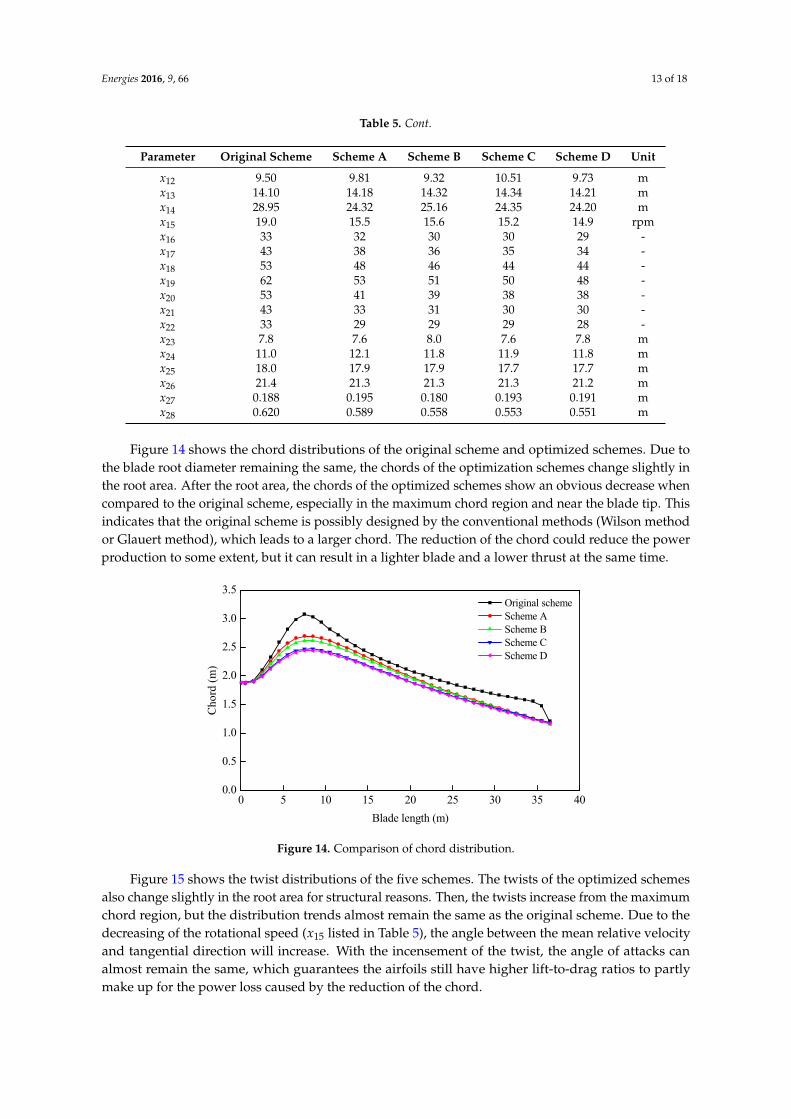
Figure 14 shows the chord distributions of the original scheme and optimized schemes. Due tothe blade root diameter remaining the same, the chords of the optimization schemes change slightly inthe root area. After the root area, the chords of the optimized schemes show an obvious decrease whencompared to the original scheme, especially in the maximum chord region and near the blade tip. Thisindicates that the original scheme is possibly designed by the conventional methods (Wilson methodor Glauert method), which leads to a larger chord. The reduction of the chord could reduce the powerproduction to some extent, but it can result in a lighter blade and a lower thrust at the same time.
Energies 2016, 9, 66 13 of 18
Figure 14 shows the chord distributions of the original scheme and optimized schemes. Due to
the blade root diameter remaining the same, the chords of the optimization schemes change slightly
in the root area. After the root area, the chords of the optimized schemes show an obvious decrease
when compared to the original scheme, especially in the maximum chord region and near the blade
tip. This indicates that the original scheme is possibly designed by the conventional methods
(Wilson method or Glauert method), which leads to a larger chord. The reduction of the chord
could reduce the power production to some extent, but it can result in a lighter blade and a lower
thrust at the same time.
0 5 10 15 20 25 30 35 400.0
0.5
1.0
1.5
2.0
2.5
3.0
3.5
Cho
rd (
m)
Blade length (m)
Original scheme Scheme A Scheme B Scheme C Scheme D
Figure 14. Comparison of chord distribution.
Figure 15 shows the twist distributions of the five schemes. The twists of the optimized
schemes also change slightly in the root area for structural reasons. Then, the twists increase from
the maximum chord region, but the distribution trends almost remain the same as the original
scheme. Due to the decreasing of the rotational speed ( 15x listed in Table 5), the angle between the
mean relative velocity and tangential direction will increase. With the incensement of the twist, the
angle of attacks can almost remain the same, which guarantees the airfoils still have higher
lift‐to‐drag ratios to partly make up for the power loss caused by the reduction of the chord.
x12 9.50 9.81 9.32 10.51 9.73 m
x13 14.10 14.18 14.32 14.34 14.21 m
x14 28.95 24.32 25.16 24.35 24.20 m
x15 19.0 15.5 15.6 15.2 14.9 rpm
x16 33 32 30 30 29 ‐
x17 43 38 36 35 34 ‐
x18 53 48 46 44 44 ‐
x19 62 53 51 50 48 ‐
x20 53 41 39 38 38 ‐
x21 43 33 31 30 30 ‐
x22 33 29 29 29 28 ‐
x23 7.8 7.6 8.0 7.6 7.8 m
x24 11.0 12.1 11.8 11.9 11.8 m
x25 18.0 17.9 17.9 17.7 17.7 m
x26 21.4 21.3 21.3 21.3 21.2 m
x27 0.188 0.195 0.180 0.193 0.191 m
x28 0.620 0.589 0.558 0.553 0.551 m
Figure 14. Comparison of chord distribution.
Figure 15 shows the twist distributions of the five schemes. The twists of the optimized schemesalso change slightly in the root area for structural reasons. Then, the twists increase from the maximumchord region, but the distribution trends almost remain the same as the original scheme. Due to thedecreasing of the rotational speed (x15 listed in Table 5), the angle between the mean relative velocityand tangential direction will increase. With the incensement of the twist, the angle of attacks canalmost remain the same, which guarantees the airfoils still have higher lift-to-drag ratios to partlymake up for the power loss caused by the reduction of the chord.
Energies 2016, 9, 66 14 of 18Energies 2016, 9, 66 14 of 18
0 5 10 15 20 25 30 35 40-3
-1
1
3
5
7
9
11
13
Tw
ist ()
Blade length (m)
Original scheme Scheme A Scheme B Scheme C Scheme D
Figure 15. Comparison of twist distribution.
The percent thickness distributions are shown in Figure 16. The locations of the airfoils with
40% and 30% thicknesses for the optimized schemes move toward the tip. From the structural point
of view, this is good for increasing the section moment of inertia. The location of the airfoil with
25% thickness almost remains the same, while that of the airfoil with 18% thickness moves toward
the root. As the airfoil with 18% thickness has a higher lift‐to‐drag ratio, the aerodynamic region
composed by this airfoil is the main part of the blade to capture wind energy. Moving the location
of the airfoil with 18% thickness towards the root can increase the length of this region, which is
beneficial to capture more energy, thus improving the power efficiency from the aerodynamic point
of view. The blade shapes become much smoother after optimization, which is more convenient for
manufacturing. The decreasing of the rotational speed could reduce the rotor rotation times during
a 20 year life span, and thus improve the fatigue life of the blade.
0 5 10 15 20 25 30 35 400
20
40
60
80
100
Per
cent
thic
knes
s (%
)
Blade length (m)
Original scheme Scheme A Scheme B Scheme C Scheme D
Figure 16. Comparison of percent thickness distribution.
Figures 17 and 18 show the comparison of power coefficients and powers between the original
scheme and optimized schemes, respectively. When compared to the original scheme, the power
coefficients of the optimized schemes increase significantly in the speed range of 4 to 8 m/s, and
decrease slightly in the peed range of 10 to 13 m/s. The power coefficients of the optimized schemes
all reach the maximum values of about 0.49 at 8 m/s wind speed (a 7.7% increase compared to the
original scheme), and keep relatively high values in the speed range of 6 to 9 m/s. With the
reduction of chord, the rated wind speeds of the 4 optimized schemes gradually change from 12 to
15 m/s, as shown in Figure 15. The comparisons in Figures 17 and 18 reveal that the optimized
schemes have better aerodynamic performances than the original scheme at low wind speeds, but
the performances gradually become worse when the wind speed increases. As can be seen from
Figure 12, for a turbine site with an annual average wind speed of 6 m/s, the probabilities of the wind
Figure 15. Comparison of twist distribution.
The percent thickness distributions are shown in Figure 16. The locations of the airfoils with40% and 30% thicknesses for the optimized schemes move toward the tip. From the structural pointof view, this is good for increasing the section moment of inertia. The location of the airfoil with25% thickness almost remains the same, while that of the airfoil with 18% thickness moves towardthe root. As the airfoil with 18% thickness has a higher lift-to-drag ratio, the aerodynamic regioncomposed by this airfoil is the main part of the blade to capture wind energy. Moving the locationof the airfoil with 18% thickness towards the root can increase the length of this region, which isbeneficial to capture more energy, thus improving the power efficiency from the aerodynamic pointof view. The blade shapes become much smoother after optimization, which is more convenient formanufacturing. The decreasing of the rotational speed could reduce the rotor rotation times during a20 year life span, and thus improve the fatigue life of the blade.
Energies 2016, 9, 66 14 of 18
0 5 10 15 20 25 30 35 40-3
-1
1
3
5
7
9
11
13
Tw
ist ()
Blade length (m)
Original scheme Scheme A Scheme B Scheme C Scheme D
Figure 15. Comparison of twist distribution.
The percent thickness distributions are shown in Figure 16. The locations of the airfoils with
40% and 30% thicknesses for the optimized schemes move toward the tip. From the structural point
of view, this is good for increasing the section moment of inertia. The location of the airfoil with
25% thickness almost remains the same, while that of the airfoil with 18% thickness moves toward
the root. As the airfoil with 18% thickness has a higher lift‐to‐drag ratio, the aerodynamic region
composed by this airfoil is the main part of the blade to capture wind energy. Moving the location
of the airfoil with 18% thickness towards the root can increase the length of this region, which is
beneficial to capture more energy, thus improving the power efficiency from the aerodynamic point
of view. The blade shapes become much smoother after optimization, which is more convenient for
manufacturing. The decreasing of the rotational speed could reduce the rotor rotation times during
a 20 year life span, and thus improve the fatigue life of the blade.
0 5 10 15 20 25 30 35 400
20
40
60
80
100
Per
cent
thic
knes
s (%
)
Blade length (m)
Original scheme Scheme A Scheme B Scheme C Scheme D
Figure 16. Comparison of percent thickness distribution.
Figures 17 and 18 show the comparison of power coefficients and powers between the original
scheme and optimized schemes, respectively. When compared to the original scheme, the power
coefficients of the optimized schemes increase significantly in the speed range of 4 to 8 m/s, and
decrease slightly in the peed range of 10 to 13 m/s. The power coefficients of the optimized schemes
all reach the maximum values of about 0.49 at 8 m/s wind speed (a 7.7% increase compared to the
original scheme), and keep relatively high values in the speed range of 6 to 9 m/s. With the
reduction of chord, the rated wind speeds of the 4 optimized schemes gradually change from 12 to
15 m/s, as shown in Figure 15. The comparisons in Figures 17 and 18 reveal that the optimized
schemes have better aerodynamic performances than the original scheme at low wind speeds, but
the performances gradually become worse when the wind speed increases. As can be seen from
Figure 12, for a turbine site with an annual average wind speed of 6 m/s, the probabilities of the wind
Figure 16. Comparison of percent thickness distribution.
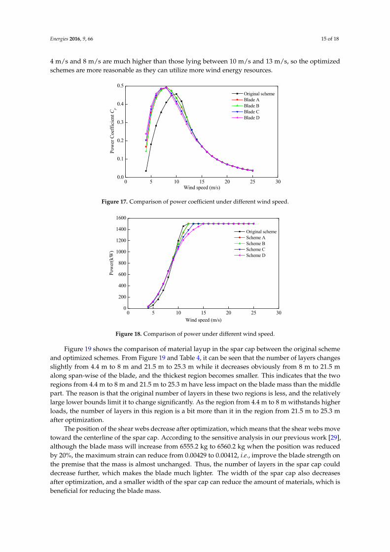
Figures 17 and 18 show the comparison of power coefficients and powers between the originalscheme and optimized schemes, respectively. When compared to the original scheme, the powercoefficients of the optimized schemes increase significantly in the speed range of 4 to 8 m/s, anddecrease slightly in the peed range of 10 to 13 m/s. The power coefficients of the optimized schemesall reach the maximum values of about 0.49 at 8 m/s wind speed (a 7.7% increase compared to theoriginal scheme), and keep relatively high values in the speed range of 6 to 9 m/s. With the reductionof chord, the rated wind speeds of the 4 optimized schemes gradually change from 12 to 15 m/s, asshown in Figure 15. The comparisons in Figures 17 and 18 reveal that the optimized schemes havebetter aerodynamic performances than the original scheme at low wind speeds, but the performancesgradually become worse when the wind speed increases. As can be seen from Figure 12, for a turbinesite with an annual average wind speed of 6 m/s, the probabilities of the wind speed lying between
Energies 2016, 9, 66 15 of 18
4 m/s and 8 m/s are much higher than those lying between 10 m/s and 13 m/s, so the optimizedschemes are more reasonable as they can utilize more wind energy resources.
Energies 2016, 9, 66 15 of 18
speed lying between 4 m/s and 8 m/s are much higher than those lying between 10 m/s and 13 m/s,
so the optimized schemes are more reasonable as they can utilize more wind energy resources.
0 5 10 15 20 25 300.0
0.1
0.2
0.3
0.4
0.5
Original scheme Blade A Blade B Blade C Blade D
Pow
er C
oeff
icie
nt Cp
Wind speed (m/s)
Figure 17. Comparison of power coefficient under different wind speed.
0 5 10 15 20 25 300
200
400
600
800
1000
1200
1400
1600
Original scheme Scheme A Scheme B Scheme C Scheme D
Pow
er(k
W)
Wind speed (m/s)
Figure 18. Comparison of power under different wind speed.
Figure 19 shows the comparison of material layup in the spar cap between the original scheme
and optimized schemes. From Figure 19 and Table 4, it can be seen that the number of layers
changes slightly from 4.4 m to 8 m and 21.5 m to 25.3 m while it decreases obviously from 8 m to
21.5 m along span‐wise of the blade, and the thickest region becomes smaller. This indicates that the
two regions from 4.4 m to 8 m and 21.5 m to 25.3 m have less impact on the blade mass than the
middle part. The reason is that the original number of layers in these two regions is less, and the
relatively large lower bounds limit it to change significantly. As the region from 4.4 m to 8 m
withstands higher loads, the number of layers in this region is a bit more than it in the region from
21.5 m to 25.3 m after optimization.
The position of the shear webs decrease after optimization, which means that the shear webs
move toward the centerline of the spar cap. According to the sensitive analysis in our previous
work [29], although the blade mass will increase from 6555.2 kg to 6560.2 kg when the position was
reduced by 20%, the maximum strain can reduce from 0.00429 to 0.00412, i.e., improve the blade
strength on the premise that the mass is almost unchanged. Thus, the number of layers in the spar
cap could decrease further, which makes the blade much lighter. The width of the spar cap also
decreases after optimization, and a smaller width of the spar cap can reduce the amount of
materials, which is beneficial for reducing the blade mass.
Figure 17. Comparison of power coefficient under different wind speed.
Energies 2016, 9, 66 15 of 18
speed lying between 4 m/s and 8 m/s are much higher than those lying between 10 m/s and 13 m/s,
so the optimized schemes are more reasonable as they can utilize more wind energy resources.
0 5 10 15 20 25 300.0
0.1
0.2
0.3
0.4
0.5
Original scheme Blade A Blade B Blade C Blade D
Pow
er C
oeff
icie
nt Cp
Wind speed (m/s)
Figure 17. Comparison of power coefficient under different wind speed.
0 5 10 15 20 25 300
200
400
600
800
1000
1200
1400
1600
Original scheme Scheme A Scheme B Scheme C Scheme D
Pow
er(k
W)
Wind speed (m/s)
Figure 18. Comparison of power under different wind speed.
Figure 19 shows the comparison of material layup in the spar cap between the original scheme
and optimized schemes. From Figure 19 and Table 4, it can be seen that the number of layers
changes slightly from 4.4 m to 8 m and 21.5 m to 25.3 m while it decreases obviously from 8 m to
21.5 m along span‐wise of the blade, and the thickest region becomes smaller. This indicates that the
two regions from 4.4 m to 8 m and 21.5 m to 25.3 m have less impact on the blade mass than the
middle part. The reason is that the original number of layers in these two regions is less, and the
relatively large lower bounds limit it to change significantly. As the region from 4.4 m to 8 m
withstands higher loads, the number of layers in this region is a bit more than it in the region from
21.5 m to 25.3 m after optimization.
The position of the shear webs decrease after optimization, which means that the shear webs
move toward the centerline of the spar cap. According to the sensitive analysis in our previous
work [29], although the blade mass will increase from 6555.2 kg to 6560.2 kg when the position was
reduced by 20%, the maximum strain can reduce from 0.00429 to 0.00412, i.e., improve the blade
strength on the premise that the mass is almost unchanged. Thus, the number of layers in the spar
cap could decrease further, which makes the blade much lighter. The width of the spar cap also
decreases after optimization, and a smaller width of the spar cap can reduce the amount of
materials, which is beneficial for reducing the blade mass.
Figure 18. Comparison of power under different wind speed.
Figure 19 shows the comparison of material layup in the spar cap between the original schemeand optimized schemes. From Figure 19 and Table 4, it can be seen that the number of layers changesslightly from 4.4 m to 8 m and 21.5 m to 25.3 m while it decreases obviously from 8 m to 21.5 malong span-wise of the blade, and the thickest region becomes smaller. This indicates that the tworegions from 4.4 m to 8 m and 21.5 m to 25.3 m have less impact on the blade mass than the middlepart. The reason is that the original number of layers in these two regions is less, and the relativelylarge lower bounds limit it to change significantly. As the region from 4.4 m to 8 m withstands higherloads, the number of layers in this region is a bit more than it in the region from 21.5 m to 25.3 mafter optimization.
The position of the shear webs decrease after optimization, which means that the shear webs movetoward the centerline of the spar cap. According to the sensitive analysis in our previous work [29],although the blade mass will increase from 6555.2 kg to 6560.2 kg when the position was reducedby 20%, the maximum strain can reduce from 0.00429 to 0.00412, i.e., improve the blade strength onthe premise that the mass is almost unchanged. Thus, the number of layers in the spar cap coulddecrease further, which makes the blade much lighter. The width of the spar cap also decreasesafter optimization, and a smaller width of the spar cap can reduce the amount of materials, which isbeneficial for reducing the blade mass.
Energies 2016, 9, 66 16 of 18Energies 2016, 9, 66 16 of 18
0 5 10 15 20 25 3025
30
35
40
45
50
55
60
65
Num
ber
of la
yers
Blade length (m)
Original scheme Scheme A Scheme B Scheme C Scheme D
Figure 19. Comparison of material layup of the spar cap.
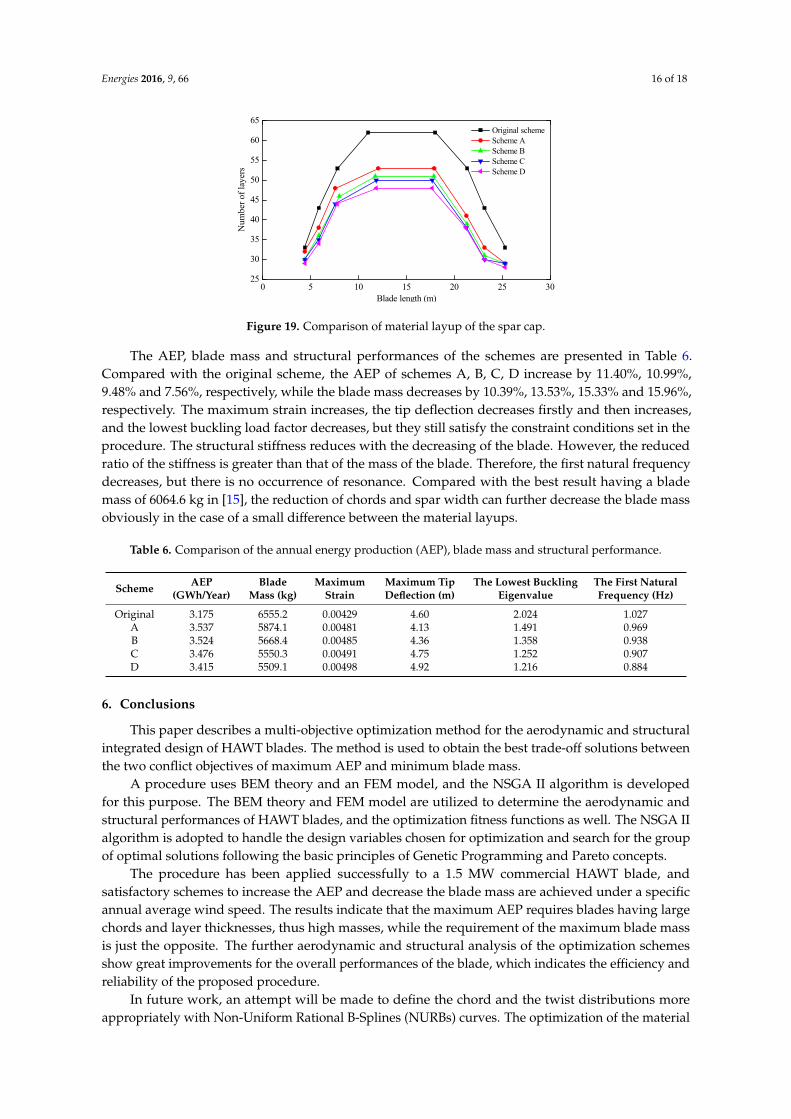
The AEP, blade mass and structural performances of the schemes are presented in Table 6.
Compared with the original scheme, the AEP of schemes A, B, C, D increase by 11.40%, 10.99%,
9.48% and 7.56%, respectively, while the blade mass decreases by 10.39%, 13.53%, 15.33% and
15.96%, respectively. The maximum strain increases, the tip deflection decreases firstly and then
increases, and the lowest buckling load factor decreases, but they still satisfy the constraint conditions
set in the procedure. The structural stiffness reduces with the decreasing of the blade. However, the
reduced ratio of the stiffness is greater than that of the mass of the blade. Therefore, the first natural
frequency decreases, but there is no occurrence of resonance. Compared with the best result having
a blade mass of 6064.6 kg in [15], the reduction of chords and spar width can further decrease the
blade mass obviously in the case of a small difference between the material layups.
Table 6. Comparison of the annual energy production (AEP), blade mass and structural performance.
Scheme AEP
(GWh/Year)
Blade
Mass (kg)
Maximum
Strain
Maximum Tip
Deflection (m)
The Lowest
Buckling
Eigenvalue
The First
Natural
Frequency (Hz)
Original 3.175 6555.2 0.00429 4.60 2.024 1.027
A 3.537 5874.1 0.00481 4.13 1.491 0.969
B 3.524 5668.4 0.00485 4.36 1.358 0.938
C 3.476 5550.3 0.00491 4.75 1.252 0.907
D 3.415 5509.1 0.00498 4.92 1.216 0.884
6. Conclusions
This paper describes a multi‐objective optimization method for the aerodynamic and structural
integrated design of HAWT blades. The method is used to obtain the best trade‐off solutions
between the two conflict objectives of maximum AEP and minimum blade mass.
A procedure uses BEM theory and an FEM model, and the NSGA II algorithm is developed for
this purpose. The BEM theory and FEM model are utilized to determine the aerodynamic and
structural performances of HAWT blades, and the optimization fitness functions as well. The NSGA
II algorithm is adopted to handle the design variables chosen for optimization and search for the
group of optimal solutions following the basic principles of Genetic Programming and Pareto concepts.
The procedure has been applied successfully to a 1.5 MW commercial HAWT blade, and
satisfactory schemes to increase the AEP and decrease the blade mass are achieved under a specific
annual average wind speed. The results indicate that the maximum AEP requires blades having
large chords and layer thicknesses, thus high masses, while the requirement of the maximum blade
mass is just the opposite. The further aerodynamic and structural analysis of the optimization
schemes show great improvements for the overall performances of the blade, which indicates the
efficiency and reliability of the proposed procedure.
In future work, an attempt will be made to define the chord and the twist distributions more
appropriately with Non‐Uniform Rational B‐Splines (NURBs) curves. The optimization of the
Figure 19. Comparison of material layup of the spar cap.
The AEP, blade mass and structural performances of the schemes are presented in Table 6.Compared with the original scheme, the AEP of schemes A, B, C, D increase by 11.40%, 10.99%,9.48% and 7.56%, respectively, while the blade mass decreases by 10.39%, 13.53%, 15.33% and 15.96%,respectively. The maximum strain increases, the tip deflection decreases firstly and then increases,and the lowest buckling load factor decreases, but they still satisfy the constraint conditions set in theprocedure. The structural stiffness reduces with the decreasing of the blade. However, the reducedratio of the stiffness is greater than that of the mass of the blade. Therefore, the first natural frequencydecreases, but there is no occurrence of resonance. Compared with the best result having a blademass of 6064.6 kg in [15], the reduction of chords and spar width can further decrease the blade massobviously in the case of a small difference between the material layups.
Table 6. Comparison of the annual energy production (AEP), blade mass and structural performance.
Scheme AEP(GWh/Year)
BladeMass (kg)
MaximumStrain
Maximum TipDeflection (m)
The Lowest BucklingEigenvalue
The First NaturalFrequency (Hz)
Original 3.175 6555.2 0.00429 4.60 2.024 1.027A 3.537 5874.1 0.00481 4.13 1.491 0.969B 3.524 5668.4 0.00485 4.36 1.358 0.938C 3.476 5550.3 0.00491 4.75 1.252 0.907D 3.415 5509.1 0.00498 4.92 1.216 0.884
6. Conclusions
This paper describes a multi-objective optimization method for the aerodynamic and structuralintegrated design of HAWT blades. The method is used to obtain the best trade-off solutions betweenthe two conflict objectives of maximum AEP and minimum blade mass.
A procedure uses BEM theory and an FEM model, and the NSGA II algorithm is developedfor this purpose. The BEM theory and FEM model are utilized to determine the aerodynamic andstructural performances of HAWT blades, and the optimization fitness functions as well. The NSGA IIalgorithm is adopted to handle the design variables chosen for optimization and search for the groupof optimal solutions following the basic principles of Genetic Programming and Pareto concepts.
The procedure has been applied successfully to a 1.5 MW commercial HAWT blade, andsatisfactory schemes to increase the AEP and decrease the blade mass are achieved under a specificannual average wind speed. The results indicate that the maximum AEP requires blades having largechords and layer thicknesses, thus high masses, while the requirement of the maximum blade massis just the opposite. The further aerodynamic and structural analysis of the optimization schemesshow great improvements for the overall performances of the blade, which indicates the efficiency andreliability of the proposed procedure.
In future work, an attempt will be made to define the chord and the twist distributions moreappropriately with Non-Uniform Rational B-Splines (NURBs) curves. The optimization of the material
Energies 2016, 9, 66 17 of 18
layup in the whole spar cap will also be carried out to further improve the overall performances ofthe blade.
Acknowledgments: This work is financially supported by the key disciplines of Zhejiang Province-BuildingEnergy Saving Technology (Grant No. 71012005Z-2).
Author Contributions: Jie Zhu carried out most of the work presented here, Xin Cai was the supervisors of thiswork, and Rongrong Gu had a relevant contribution with her extensive knowledge about the FEM modeling ofthe blade.
Conflicts of Interest: The authors declare no conflict of interest.
References
1. BTM Consult. World Wind Energy Market Update 2015; BTM Consult: Chicago, IL, USA, 2015.2. Burton, T.; Jenkins, N.; Sharpe, D.; Bossanyi, E. Wind Energy Handbook; John Wiley & Sons: Chichester,
West Sussex, UK, 2011.3. Kim, B.; Kim, W.; Lee, S.; Bae, S.; Lee, Y. Developement and verification of a performance based optimal
design software for wind turbine blades. Renew. Energy 2013, 54, 166–172. [CrossRef]4. Xudong, W.; Shen, W.Z.; Zhu, W.J.; Sørensen, J.N.; Jin, C. Shape optimization of wind turbine blades.
Wind Energy 2009, 12, 781–803. [CrossRef]5. Kusiak, A.; Zheng, H. Optimization of wind turbine energy and power factor with an evolutionary
computation algorithm. Energy 2010, 35, 1324–1332. [CrossRef]6. Sharifi, A.; Nobari, M.R. Prediction of optimum section pitch angle distribution along wind turbine blades.
Energ. Convers. Manag. 2013, 67, 342–350. [CrossRef]7. Maalawi, K.Y.; Badr, M.A. Frequency optimization of a wind turbine blade in pitching motion. P. I. Mech.
Eng. A 2010, 224, 545–554. [CrossRef]8. Dal Monte, A.; Castelli, M.R.; Benini, E. Multi-objective structural optimization of a HAWT composite blade.
Compos. Struct. 2013, 106, 362–373. [CrossRef]9. Chen, J.; Wang, Q.; Shen, W.Z.; Pang, X.; Li, S.; Guo, X. Structural optimization study of composite wind
turbine blade. Mater. Des. 2013, 46, 247–255. [CrossRef]10. Grujicic, M.; Arakere, G.; Pandurangan, B.; Sellappan, V.; Vallejo, A.; Ozen, M. Multidisciplinary design
optimization for glass-fiber epoxy-matrix composite 5 MW horizontal-axis wind-turbine blades. J. Mater.Eng. Perform. 2010, 19, 1116–1127. [CrossRef]
11. Bottasso, C.L.; Campagnolo, F.; Croce, A. Multi-disciplinary constrained optimization of wind turbines.Multibody Syst. Dyn. 2012, 27, 21–53. [CrossRef]
12. Benini, E.; Toffolo, A. Optimal design of horizontal-axis wind turbines using blade-element theory andevolutionary computation. J. Sol. Energ. 2002, 124, 357–363. [CrossRef]
13. Wang, L.; Wang, T.G.; Luo, Y. Improved non-dominated sorting genetic algorithm (NSGA)-II inmulti-objective optimization studies of wind turbine blades. Appl. Math. Mech Engl. 2011, 32, 739–748.[CrossRef]
14. Wang, T.; Wang, L.; Zhong, W.; Xu, B.; Chen, L. Large-scale wind turbine blade design and aerodynamicanalysis. Chin. Sci. Bull. 2012, 57, 466–472. [CrossRef]
15. Cai, X.; Zhu, J.; Pan, P.; Gu, R. Structural optimization design of horizontal-axis wind turbine blades using aparticle swarm optimization algorithm and finite element method. Energies 2012, 5, 4683–4696. [CrossRef]
16. Cairns, D.S.; Mandell, J.; Combs, D.C.; Rabern, D.A.; van Luchene, R.D. Analysis of a Composite Blade Designfor the AOC 15/50 Wind Turbine Using a Finite Element Model; Sandia National Laboratories: Albuquerque,NM, USA, 2001.
17. Locke, J.; Valencia, U.; Ishikawa, K. Design studies for twist-coupled wind turbine blades. In Proceedings ofthe ASME 2003 Wind Energy Symposium, Reno, NV, USA, 6–9 January 2003; American Society of MechanicalEngineers: Wichita, KS, USA, 2003; pp. 324–331.
18. Spera, D.A. Wind Turbine Technology; American Society of Mechanical Engineers: Fairfield, NJ, USA, 1994.19. Gasch, R.; Twele, J. Wind Power Plants: Fundamentals, Design, Construction and Operation; Springer Science &
Business Media: Berlin, Germany, 2011.20. Hansen, M.O. Aerodynamics of Wind Turbines; Routledge: New York, NY, USA, 2015.
Energies 2016, 9, 66 18 of 18
21. Ashwill, T.D. Cost Study for Large Wind Turbine Blades: WindPACT Blade System Design Studies(No. SAND2003-1428); Sandia National Labs.: Albuquerque, NM, USA; Livermore, CA, USA, 2003.
22. Buckney, N.; Pirrera, A.; Green, S.D.; Weaver, P.M. Structural efficiency of a wind turbine blade.Thin-Wall Struct. 2013, 67, 144–154. [CrossRef]
23. Lee, Y.J.; Jhan, Y.T.; Chung, C.H. Fluid-structure interaction of FRP wind turbine blades under aerodynamiceffect. Compos. Part B 2012, 43, 2180–2191. [CrossRef]
24. Liao, C.C.; Zhao, X.L.; Xu, J.Z. Blade layers optimization of wind turbines using FAST and improved PSOalgorithm. Renew. Energy 2012, 42, 227–233. [CrossRef]
25. Jureczko, M.E.; Pawlak, M.; Mezyk, A. Optimisation of wind turbine blades. J. Mater. Proc. Technol. 2005, 167,463–471. [CrossRef]
26. Deb, K.; Pratap, A.; Agarwal, S.; Meyarivan, T. A fast and elitist multiobjective genetic algorithm: NSGA-II.IEEE Trans. Evol. Comput. 2002, 6, 182–197. [CrossRef]
27. Serrano, V.; Alvarado, M.; Coello, C.A. Optimization to manage supply chain disruptions using the NSGA-II.In Theoretical Advances and Applications of Fuzzy Logic and Soft Computing; Springer: Berlin/Heidelberg,Germany, 2007; pp. 476–485.
28. Palanikumar, K.; Latha, B.; Senthilkumar, V.S.; Karthikeyan, R. Multiple performance optimization inmachining of GFRP composites by a PCD tool using non-dominated sorting genetic algorithm (NSGA-II).Metal Mater. Int. 2009, 15, 249–258. [CrossRef]
29. Zhu, J.; Cai, X.; Pan, P.; Gu, R. Multi-objective structural optimization design of horizontal-axis wind turbineblades using the non-dominated sorting genetic algorithm II and finite element method. Energies 2014, 7,988–1002. [CrossRef]
© 2016 by the authors; licensee MDPI, Basel, Switzerland. This article is an open accessarticle distributed under the terms and conditions of the Creative Commons by Attribution(CC-BY) license (http://creativecommons.org/licenses/by/4.0/).


