i
ADMISSION CONTROL AND RESOURCE RESERVATION FOR QUALITY OFSERVICE PROVISIONING IN CELLULAR MOBILE WIRELESS NETWORKS
A Thesis
Presented to
The Faculty of the Department of Electrical and Computer Engineering
University of Houston
In Partial Fulfillment
of the Requirements for the Degree
Master of Science
in Electrical Engineering
by
Kashif Shakil
October 2001

ii
ADMISSION CONTROL AND RESOURCE RESERVATION FOR QUALITY OFSERVICE PROVISIONING IN CELLULAR MOBILE WIRELESS NETWORKS
Kashif Shakil
Approved:
Chariman of the CommitteeLennart Johnsson, Professor,
Electrical and Computer Engineering, Computer Science
Committee Members:
Wallace Anderson, Professor,Electrical and Computer Engineering
David Pai, Associate ProfessorElectrical and Computer Engineering
E. Joseph Charlson, Associate Dean Fritz Claydon, Professor and ChairmanCullen College of Engineering Electrical and Computer Engineering

iii
Acknowledgements
I would like to thank Dr. Lennart Johnsson for his continued advice and guidance
through the development of this thesis. Thanks also to Dr. Wallace Anderson for
his valuable support. Finally, I am very grateful to Dr. Edward Knightly and his
research group at Rice University for their guidance and suggestions that went
into the development of the ideas in this work.
iv
ADMISSION CONTROL AND RESOURCE RESERVATION FOR QUALITY OFSERVICE PROVISIONING IN CELLULAR MOBILE WIRELESS NETWORKS
An Abstract
of a
Thesis
Presented to
The Faculty of the Department of Electrical and Computer Engineering
University of Houston
In Partial Fulfillment
of the Requirements for the Degree
Master of Science
in Electrical Engineering
by
Kashif Shakil
October 2001

v
Abstract
In this thesis we propose a new admission control and resource reservation
scheme for microcellular multimedia mobile PCS networks. This scheme takes
advantage of the user to user correlation of user mobility characteristics and forms
aggregate spatial flows from individual users. Spatial flows of mobile users can
be utilized for making bandwidth reservation for provision of desired quality of
service (QoS). The overall scheme has been designed to minimize the amount of
computation required per user for its QoS demand. At the same time, our aim is to
maintain an appreciable level of accuracy in admission control decisions.
Furthermore, our mobility classification scheme is suitable for the periodic
variations of user mobility characteristics due to time of the day and day of the
week. We perform an extensive set of simulations to show that our algorithm
achieves a QoS performance that is comparable to the performance of some more
computationally intensive schemes. Our algorithm keeps the system resource
utilization at a high level, while maintaining the QoS performance. We also show
that the computational complexity of our algorithm is more than 103 times better
than algorithms with comparable QoS performance.
vi
TABLE OF CONTENTS
1. INTRODUCTION ................................................................................................................. 1
2. MOBILITY CLASSIFICATION METHODOLOGY..................................................... 13
2.1 DECISION TREE APPROACH.............................................................................................. 162.2 CLASS DISCOVERY ............................................................................................................ 192.3 CLASS SPECIFICATION ....................................................................................................... 232.4 USER CLASSIFICATION....................................................................................................... 262.5 MOBILITY CLASSIFICATION ALGORITHM .......................................................................... 312.6 SECTION SUMMARY ........................................................................................................... 35
3. MOBILITY SPATIAL FLOW FRAMEWORK .............................................................. 37
3.1 TWO DIMENSIONAL SPATIAL FLOW MODEL...................................................................... 393.2 ONE DIMENSIONAL FLOW MODEL .................................................................................... 533.3 SECTION SUMMARY ........................................................................................................... 56
4. QUALITY OF SERVICE WITH SPATIAL FLOWS ..................................................... 57
4.1 HANDOFF SCHEME............................................................................................................. 604.2 RESOURCE RESERVATION SCHEME ................................................................................... 654.3 ADMISSION CONTROL ALGORITHM ................................................................................... 734.4 SECTION SUMMARY ........................................................................................................... 79
5. RELATED WORK WITH COMPARISONS................................................................... 81
6. SIMULATION EXPERIMENTS....................................................................................... 89
6.1 EXPERIMENTS WITH SCA .................................................................................................. 926.2 EXPERIMENTS WITH SPATIAL FLOWS ALGORITHM ........................................................ 103
7. CONCLUSION .................................................................................................................. 122
8. REFERENCES .................................................................................................................. 125

vii
LIST OF FIGURES
FIGURE 1: SCATTER PLOT AND HISTOGRAM OF CELL RESIDENCE TIME DATA FROM BAY AREA
MARKET. ................................................................................................................................ 13FIGURE 2: EQUALLY PARTITIONED 3-DIMENSIONAL PARAMETER SPACE AND THE ASSOCIATED
DECISION TREE. ...................................................................................................................... 17FIGURE 3: PSEUDO-CODE FOR CLASS DISCOVERY USING H-PROCEDURE. ..................................... 22FIGURE 4: PSEUDO-CODE FOR MOBILITY CLASSIFICATION ALGORITHM. ...................................... 33FIGURE 5: TWO DIMENSIONAL CELL GRID AND ASSOCIATED FLOW MODEL.................................. 39FIGURE 6: ROOT, BRANCHING, RESIDUAL, DISSIPATIVE AND GENERATING FLOWS IN CELL 0/
NEIGHBORS. ........................................................................................................................... 40FIGURE 7: ONE DIMENSIONAL SERVICE AREA MODEL WITH SPATIAL FLOWS. .............................. 53FIGURE 8: USERS IN TRANSITION REGION WITH URGENT OR NON-URGENT HANDOFFS. ............... 61FIGURE 9: PSEUDO-CODE FOR HANDOFF SCHEME. ........................................................................ 63FIGURE 10: PSEUDO-CODE FOR ADMISSION CONTROL SCHEME. ................................................... 77FIGURE 11: QOS PARAMETERS AND AVERAGE UTILIZATION VS. REJECTION THRESHOLD FOR SCA.
............................................................................................................................................... 95FIGURE 12: QOS PARAMETERS AND AVERAGE UTILIZATION VS. AVAILABLE CAPACITY FOR SCA.
............................................................................................................................................... 96FIGURE 13: QOS PARAMETERS / AVERAGE UTILIZATION VS. MEAN CALL INTER-ARRIVAL TIME
FOR SCA. ............................................................................................................................... 98FIGURE 14: QOS PARAMETERS AND AVERAGE UTILIZATION VS. PROJECTION INTERVAL FOR SCA.
............................................................................................................................................. 100FIGURE 15: QOS PARAMETER AND AVERAGE UTILIZATION VS. ALGORITHM STEP SIZE FOR SCA.
............................................................................................................................................. 101FIGURE 16: QOS PARAMETERS / UTILIZATION VS. MEAN AGGREGATE CELL RESIDENCE TIME FOR
SCA. .................................................................................................................................... 102FIGURE 17: QOS PARAMETERS AND UTILIZATION VS. NORMALIZED RESERVATION PERIOD FOR
SFA...................................................................................................................................... 104FIGURE 18: QOS PARAMETERS AND UTILIZATION VS. RESERVATION GAIN FOR SFA................. 105FIGURE 19: QOS PARAMETERS AND UTILIZATION VS. ADMISSIBILITY CONSTANT FOR SFA. ..... 106FIGURE 20: QOS PARAMETERS AND UTILIZATION VS. SURVIVABILITY CONSTANT FOR SFA. .... 108FIGURE 21: QOS PARAMETER AND UTILIZATION VS. AVAILABLE CAPACITY FOR SFA............... 110FIGURE 22: QOS PARAMETERS AND UTILIZATION VS. MEAN CALL INTER-ARRIVAL TIME FOR SFA.
............................................................................................................................................. 111FIGURE 23: QOS PARAMETER AND UTILIZATION VS. HANDOFF URGENCY FACTOR FOR SFA..... 113FIGURE 24: QOS PARAMETERS AND UTILIZATION VS. ALGORITHM STEP SIZE FOR SFA............. 114FIGURE 25: QOS PARAMETERS AND UTILIZATION VS. PROJECTION INTERVAL OF SFA.............. 116
1
1. INTRODUCTION
Third generation mobile cellular systems will provide multimedia services to a
large number of users. Since multimedia traffic may have a great amount of
information content, users will demand much higher bandwidth than currently
available for circuit-switched voice. Multimedia traffic is also bursty in nature,
which means that the bandwidth requirement for each user will change with time.
Combine this with the fact that each user may request bandwidth and additional
resources differently than other users, we get a highly heterogeneous mix of
space-time varying traffic. In addition, multimedia forms mostly real-time traffic
and thus it is delay sensitive. Providing sufficient resources to the users over a
period of time is a complex problem. An easy approach to solving this problem is
to transport multimedia traffic over circuit switched connections, analogous to
voice over POTS. This is not always an optimum solution because of greater
wastage of resources and management effort. Even if the air interface is circuit
switched in nature, the underlying network may be packet-based. Thus there will
arise a need to address QoS issues uniformly over the entire network. Knightly
and Schroff [1] have given a summary of the most important stochastic admission
approaches. Schroff et al [2] describe the fundamental limitations on deterministic
techniques of QoS guarantees. They show that only very low resource utilization
is possible with deterministic QoS. New and innovative service disciplines need
to be defined to support these QoS techniques [3], [4].

2
The kind of traffic on the network basically determines the network architecture.
Beyond traffic stream level issues, the greater bandwidth requirement per user
forces cell size to become smaller. In the future cellular systems, a hierarchical
cell structure may be used [5], but majority of the cells are expected to support
slow moving users accessing high bandwidth services. These cells would be of
small radius of less than 500 meters diameter - microcells, so that more users can
be accommodated per unit area. The limited radio spectrum available for
cellular/PCS applications also reinforces the need for a microcellular architecture.
Handoff management is a major issue in multimedia microcellular systems. The
number of handoffs increases with smaller cell size. Bandwidth demand moves
along with the users and has to be supported in different cells and also the
underlying network infrastructure.
3
On the level of the cell , it is important to maintain connections once the calls are
accepted. Calls may be dropped or experience large delays in receiving the
required quali ty of service when handing off fr om one cell to another because of
the non-availabili ty of resources in the new cells. This may happen from time to
time but our objective is to keep handoff failure events very rare. A good measure
of the quali ty of service would be the percentage of calls dropped due to handoff
failures. We define a call dropping probability representing the probabili ty that a
handoff fails from the system's inabili ty to assign resources in the new cell . In a
conventional landline telephone system, we define quali ty of service in terms of
call blocking probability. It represents the proportion of new call requests that are
blocked because the trunks in the network are all busy serving other calls. Using
simple queueing analysis, we can derive Erlang-B or Erlang-C formulas [28].
These formulas have been traditionally used by carriers to provide trunks and
other resources to their users. In cell phone systems, further complications are
introduced by mobili ty of the users. Sudden overloading can occur in some cells
and call blocking may increase in an unprecedented manner. User mobili ty must
be taken into account when evaluating the blocking probabili ty. We would like to
attain a given call dropping probabili ty while at the same time minimizing the
blocking probabili ty. In a cellular mobile system, the blocking performance
achieved is inferior to that of a wireline phone system with the same amount of
available resources. This is due to the additional strain caused by the random
nature of user mobili ty [26].

4
To achieve the desired quality of service metrics, it is essential to reserve
resources in all the cells a user might visit in one session [23, 24, 25]. The
different schemes of making this kind of bandwidth reservation for new calls or
handoff calls are discussed in [6]. On one hand there are fixed reservation
approaches [7], [8], also called guard channel approaches. Guard channels
provide a way of prioritizing handing off calls on new call originations by setting
aside a fixed bandwidth to support handing off users. New call originations
cannot be assigned bandwidth from the guard channel pool. Additionally, handoff
calls are moved away from the guard channel pool quickly after handoffs have
completed. Guard channels have been shown to improve performance
considerably from non-reservation schemes [9]. In non-reservation schemes,
handoff calls may be dropped if the destination cell is fully loaded. Fixed
reservation has its limitations. In the third generation system where user mobility
and bandwidth demand are highly heterogeneous, fixed reservation [9]
performance degrades. Furthermore, fixed reservation can only be used to
improve performance, but it cannot give solid guarantees on the QoS metrics of
the system. We need some kind of adaptive reservation where capacity is reserved
dynamically in response to anticipated user demands. There are quite a few
approaches in the literature that perform adaptive reservation. As pointed out by
Jain and Knightly [11], all of these approaches differ in the amount of information
they need and the accuracy of required bandwidth estimation. Methods vary from
those using single user techniques to those employing some kind of aggregation.
Then there are cell occupancy models and user mobility models. Whereas cell

5
occupancy models treat occupied capacity in a cell separately from user
movements, user mobility techniques explicitly model the mobility of the users
[11] in resource reservation algorithms. As algorithms move from coarse (like
aggregate cell occupancy method) to finely granular approaches (like per-user
mobility models), there is an increase in algorithmic complexity and
computational intensiveness. There is a corresponding increase in accuracy of
bandwidth estimation.

6
As a consequence of prioritizing user handoffs over new call requests, there is an
increased incidence of new calls getting blocked [7]. Here we assume that new
calls that do not find their requested bandwidth are not queued but rather cleared.
The algorithm checks for available capacity in the cell, after subtracting capacity
reserved for handoff calls, and if there is not enough to support the new call
request that call is blocked (cleared). This procedure comprises a simple
admission control test. So in effect, we are accepting new calls only after setting
aside bandwidth for calls already admitted in other cells that are expected to
handoff to the current cell in future time. This way, we prioritize handoffs over
new call admissions. More elaborate admission control procedures can be laid out
- procedures that, for example, check for expectancy that the new user will be able
to complete its call without suffering a handoff failure. However complicated an
admission test may be, its performance necessarily depends on the reservation
scheme. We do not want the admission test to yield very conservative results
because that means that many more calls would be blocked unnecessarily, thus
degrading call blocking performance of the algorithm. On the other hand, a loose
test would result in an excessively large number of handoff failures. A loose test
would let in more users than can be supported and would cause bandwidth
starvation for already admitted users. A good admission control algorithm should
lie within these two extremes. Jain and Knightly [11] have presented a perfect
knowledge algorithm which produces the best achievable performance. No other
procedure can yield better resource utilization than this algorithm since it uses

7
future knowledge of the users' whereabouts in a cell system, which is not
available to other implementable algorithms.
Admission control of new calls and resource reservation for already admitted calls
forms the framework for providing cell l evel quality of service to users in a
wireless cellular system. In this thesis, we are not concerned with bit stream
issues. Those issues should be addressed at another level. In a real system,
admission control should be a two part process. The first part of the admission
control procedure would test for admissibili ty of multimedia traff ic streams in the
radio link as well as the underlying network infrastructure. The other part of the
admission test looks for the cell l evel admissibili ty of the user according to its
bandwidth demand, current load in the cell and mobili ty of all the users in the cell
system. In this thesis, our scope is limited to the second part of admission control.
For the sake of simplicity, we assume a fixed bandwidth allocation for each user.
Users demand a fixed bandwidth and the network endeavors to deliver it.
Whatever mechanism is initiated to decide about the bandwidth needed for a
particular stream and all the multiplexing issues are beyond the scope of this
thesis. However, it is possible to recognize the differences in QoS requirements
for different service types. For delay-tolerant applications (li ke file transfers), the
system may queue a handoff until the time when resources become available in
the new cell [10]. Thus, the network may accommodate much larger number of
connections with looser QoS requirements.

8
Models of user mobility effect the performance of admission control algorithms.
If models are exact, the algorithm is expected to yield improved performance.
With regards to modeling the user motion in a cellular system, the first important
thing is a model of service area. In the real world, cells are irregular in size and
shape. Local propagation conditions, traffic demand and physical layer issues
determine the layout of cells. In theory, considering all such factors makes the
problem analytically intractable. Simple but accurate models are therefore,
desired. Both one-dimensional and two-dimensional cell models are useful.
Regularly sized and uniformly shaped cells are used. It is possible to model the
service area with varying degrees of detail, depending on the scope of the study
[12]. Simpler models, such as a matrix of rectangular cells, are very useful in
simulation studies. To make these simple models more realistic, we can add
details like travel paths to represent roadways or pathways of the real world.
Psychophysical and social aspects of human behavior can serve as guide when
modeling user mobility. For instance, the downtown mobility model mimics a
city. Users move towards a city center in the morning hours and back to the
suburbs in the evenings. Users tend to take the shortest paths (time or distance) to
their destinations, using main roadways first and then taking the secondary paths.
Travel speed is in direct proportion to the traffic congestion and minimum head
distance requirement on the roadways [12].

9
One important parameter in modeling user mobility is the cell residence time. It is
the time spent by a user in a single cell before handing off or terminating its call.
Statistical and analytical work can reveal insight into the nature of this parameter.
Both Zonoozi et al [13] and have shown that cell residence time follows a
generalized gamma distribution. Rappaport [14] furnishes expressions for cell
residence time distribution, given generalized distributions for session and dwell
times.

10
Several attempts at analysis of the user mobility in cellular system have been
made. Chao and Chen [15] model a two cell system using a continuous time
Markov Chain. Even with the unrealistic case of a two cell system, they run into
state space explosion problems, which they partially solve by a state decoupling
technique. The approach in [16] has the same problems. Messey [17] has explored
the use of PALM (Poisson Arrival Location Model) for evaluating mobile
wireless systems. The basic assumption in [17] is that arrival times and location of
users represent a class of waiting processes that can be expected to follow
exponential distribution. To avoid state space complexities, Naghshineh and
Acampora use a cell occupancy approach in [18]. They do not explicitly model
the dynamics of user mobility, but nevertheless come up with a straightforward
expression for calculating the cell overload probability. Levine et al [19] have
presented the shadow cluster algorithm (SCA) which looks at the problem on a
much finer scale. They model the cell to cell correlation in user mobility and at
the same time avoid expansive system states. Greater accuracy is achieved by
more emphasis on intensive computation per mobile user. The measurement-
based method of [22] is also fine-grained and tracks each mobile user. On the
other hand, the method used by Naghshineh [18] is simple but cannot be expected
to yield accurate results. Other schemes also run into either one of the categories
as explained above.
11
In this thesis, we have developed a fine-grained scheme to perform admission
control and resource reservation in a wireless mobile system. Our scheme leads to
simple and fewer computational steps, but at the same time maintains the
accuracy of a fine-grained approach. We consider the call dropping probability
Pdrop as the main QoS metric. It is desirable to maximize the utilization of system
resources. This can be achieved by admitting as many users as possible under a
given situation. The other QoS metric is the call blocking probability Pblock. Our
algorithm maintains a given Pdrop and minimizes Pblock for the given value of call
dropping probability. We proceed by laying out a scheme for establishing mobility
classes. Mobility classes group users with similar mobility characteristics. Then
we describe our algorithm for assigning users to one or the other mobility class.
Aggregate spatial flows can be formed by replacing the mobility characteristics of
a single user by its class characteristics. The aggregation is, in effect, a space-time
varying bandwidth demand entity which we call spatial classed flow. Here we
introduce an approximation, which results in reduction of computational steps in
the algorithm, but it also effects algorithm accuracy. There is a tradeoff in
computational intensiveness and approximation of mobility/time characteristics in
the spatial flow framework. We show that under certain conditions our
aggregation framework can reduce reservation computations by a factor of 1280.
In Section 5, we give a comparison of the computational demands of our
algorithm and that of [19]. Next we lay out the method of forming spatial flows
from individual users. This spatial flow method is then used to present an on-line
resource estimation and admission control algorithm. It is possible to form an off-

12
line version of our on-line algorithm, which reduces admission control to a simple
table lookup. Spatial flow algorithms take into account the periodic variations in
user mobility characteristics. Also considered is the space/time dependency of
user mobility. Finally we conduct simulation experiments to evaluate the
performance of our algorithm. Results of simulation throw valuable insight on the
performance of the algorithm and also help in finetuning adjustable parameters
that affect efficiency. We also present equivalent results obtained from simulation
experiments using the algorithm of [19] to get a measure of the relative
performance of our algorithm.
This report is organized in seven sections including this one. Section 2 covers
mobility classification methodology and in Section 3 we discuss the spatial flow
framework. In Section 4 we present the admission control and resource
reservation algorithm based on the classed spatial flow framework. In Section 5,
we give a brief coverage of related work in QoS and resource management in
wireless cellular networks. Section 6 presents the simulation experiments, results
and discussion of results. Section 7 forms the conclusion of the work.

13
2. MOBILITY CLASSIFICATION METHODOLOGY
In this section we present a method for the classification of users based on their
mobili ty characteristics. We employ both new and standard methods towards that
end.
Mobili ty classes represent groupings of user mobili ty characteristics. The
properties of a class are derived from data provided by individual users. Class
membership then assigns a worst case or average characterization to each
component member. Simpli fying the analysis of the impact of user mobili ty by
defining a few mobili ty classes is a minor approximation for several reasons.
First, there are obvious logical groupings of the users' mobili ty. There are fast
moving users, mostly automobiles on roadways, where a high degree of
correlation is manifested in user-to-user mobili ty. This points to similarities that
can be exploited to form coherent class structures. Similar correlations can also be
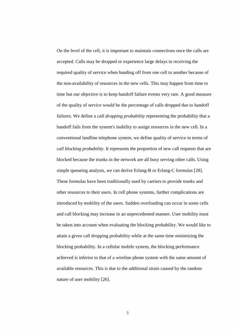
found in slow moving users, such as pedestrians. As a case in point, we have
Figure 1: Scatter plot and histogram of cell residence time data from Bay Areamarket.
0
5
10
15
20
25
30
0 200 400 600 800 1000
Sample Number
Mea
n C
ell R
esid
ence
Tim
e
0
50
100
150
200
250
1 2 3 4 5 6 7 8 9 10 11 12 13 14 15 16 17 18 19 20 21 22 23 24
Mean Cell Residence Time
Nu
mb
er o
f S
amp
les
in t
he
Bin

14
gathered cell residence time data for mobile cellular traffic in San Francisco Bay
Area provided by the Stanford University Pleiades Project [20]. The cell residence
time is measured in minutes and data is correct up to the nearest upper minute. It
can be seen that there is a clear clustering pattern at some points for cell residence
time below 5 minutes. This is also evident from the histogram.
Logically we can divide the user traffic into four different groups based on their
cell residence time; high speed users, mid speed users, slow moving users and
pseudo-stationary users. However, parameters other than the speed of a user are
also required to completely describe mobility characteristics. We introduce more
formal methods to cope with the problem of mobility classification.
15
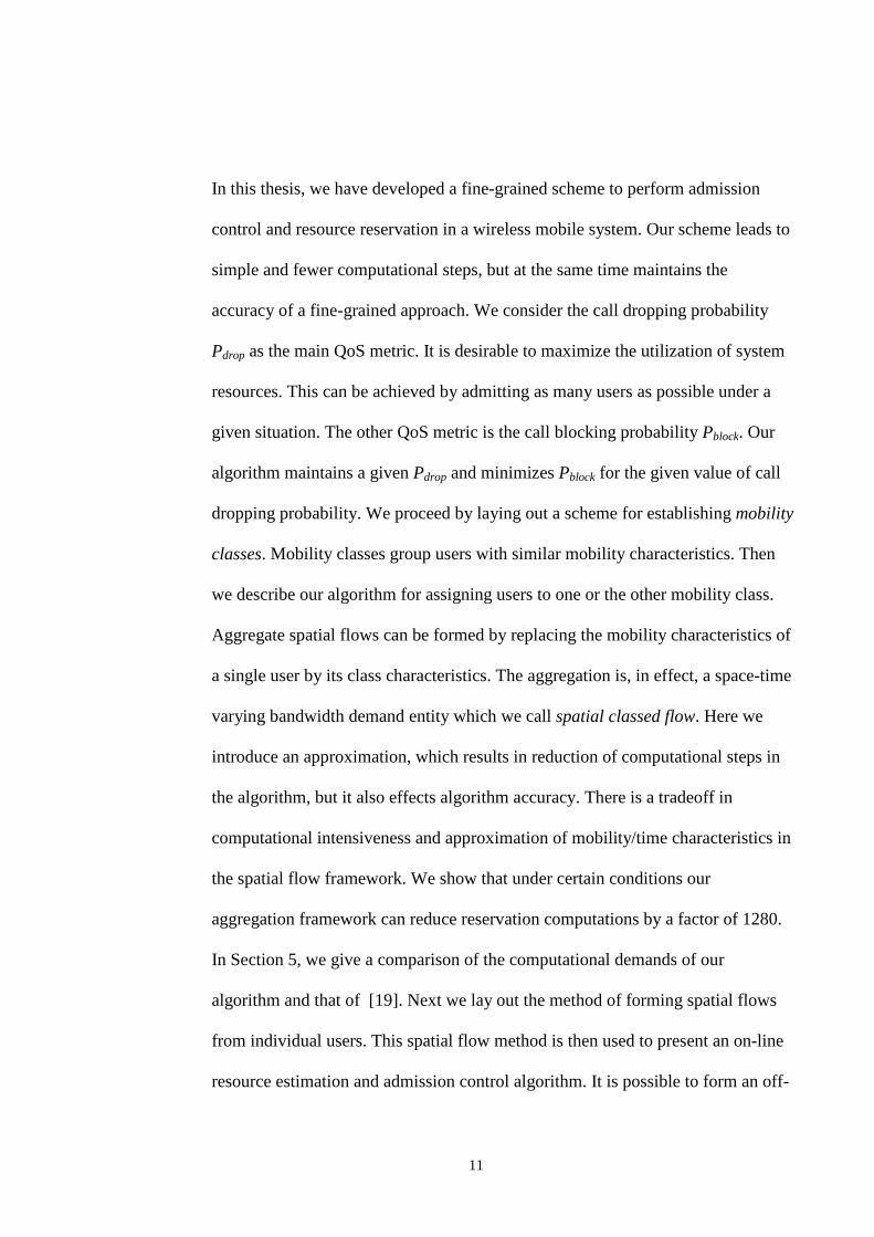
In this section, we develop a mobility classification methodology. User mobility
can be approximately described by a limited set of statistical parameters. These
parameters can be measured and refined over time as more data become available.
For instance, time spent in a cell is an important mobility parameter. Measuring
and storing the first few moments of that time is sufficient for making accurate
future predictions about the residence time in that cell. Another important
characteristic of user mobility is the handoff probability, which indicates the
probability of a user in a cell handing off to one of the neighboring cells. In this
section we assume that the mobility characteristics of a user can be represented
by a parameter vector xmob, where xmob can have as many elements as necessary to
completely specify the mobility of a user. Given a collection of vectors xmob of
multiple users, our problem is to find an optimum class structure. We use xmob of
all users in a cell to define a parameter space. The number of elements of the xmob
vector determines the dimension of the parameter space. For example, with three
elements in xmob, we get a three dimensional parameter space.
16
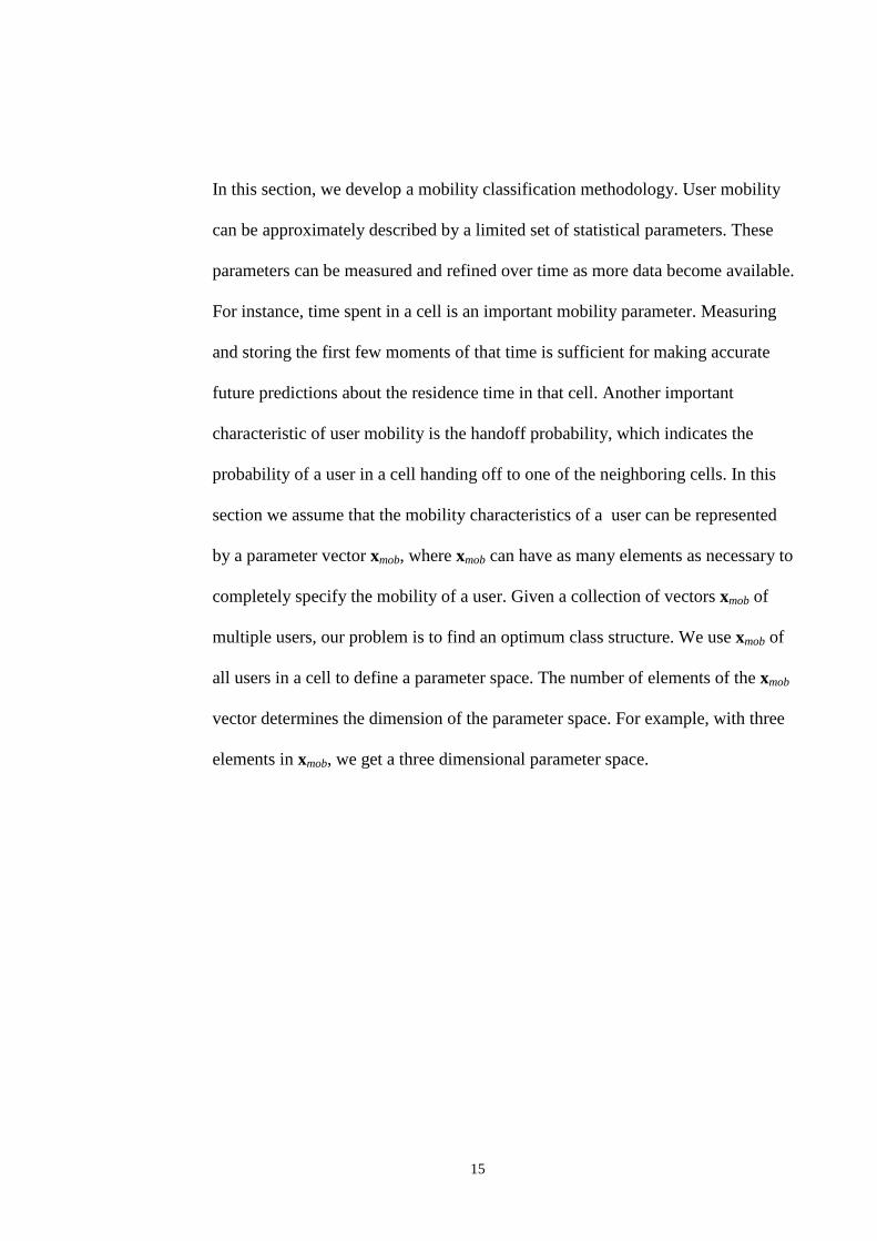
2.1 DECISION TREE APPROACH
One simple method of deciding the class membership of a user would be to form
a parameter space and partition it. This we call partitioning. Classes can be
defined by dividing the parameter space into hypercubes of predefined size. In the
example xmob with only three parameters, we can think of a three dimensional
parameter space, which we divide into identically sized cubes. The space is
completely enclosed at one end but it is open at the other end. Class membership
decisions can be formalized as a decision tree. Suppose that we divide the
parameter space into K arbitrarily and equally sized hypercubes for all parameter
dimensions and the end hypercubes being unbounded. P represents the dimension
of the parameter space, which is equal to the number of elements of xmob. The
decision tree would have K leaves. In this case, the number of hypercubes per
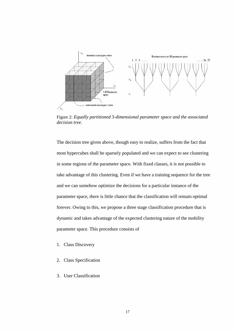
dimension of the parameter space is given by K1/P. Figure 2 shows a hypothetical
three dimensional parameter space partitioned into 27 hypercubes and its
corresponding decision tree.
17
Figure 2: Equally partitioned 3-dimensional parameter space and the associateddecision tree.
The decision tree given above, though easy to realize, suffers from the fact that
most hypercubes shall be sparsely populated and we can expect to see clustering
in some regions of the parameter space. With fixed classes, it is not possible to
take advantage of this clustering. Even if we have a training sequence for the tree
and we can somehow optimize the decisions for a particular instance of the
parameter space, there is little chance that the classification will remain optimal
forever. Owing to this, we propose a three stage classification procedure that is
dynamic and takes advantage of the expected clustering nature of the mobility
parameter space. This procedure consists of
1. Class Discovery
2. Class Specification
3. User Classification

18
Parameter space clustering may be present markedly in places where there is a
correlated movement of users. Our three stage algorithm aims at taking advantage
of the structure of the parameter space. We can also expect the structure of the
parameter space to vary with time. Time variation of the structure is addressed by
periodic invocation of class discovery and class specification algorithms. A
dynamic classification algorithm also leads to cell-to-cell differences in class
structure.
19
2.2 CLASS DISCOVERY
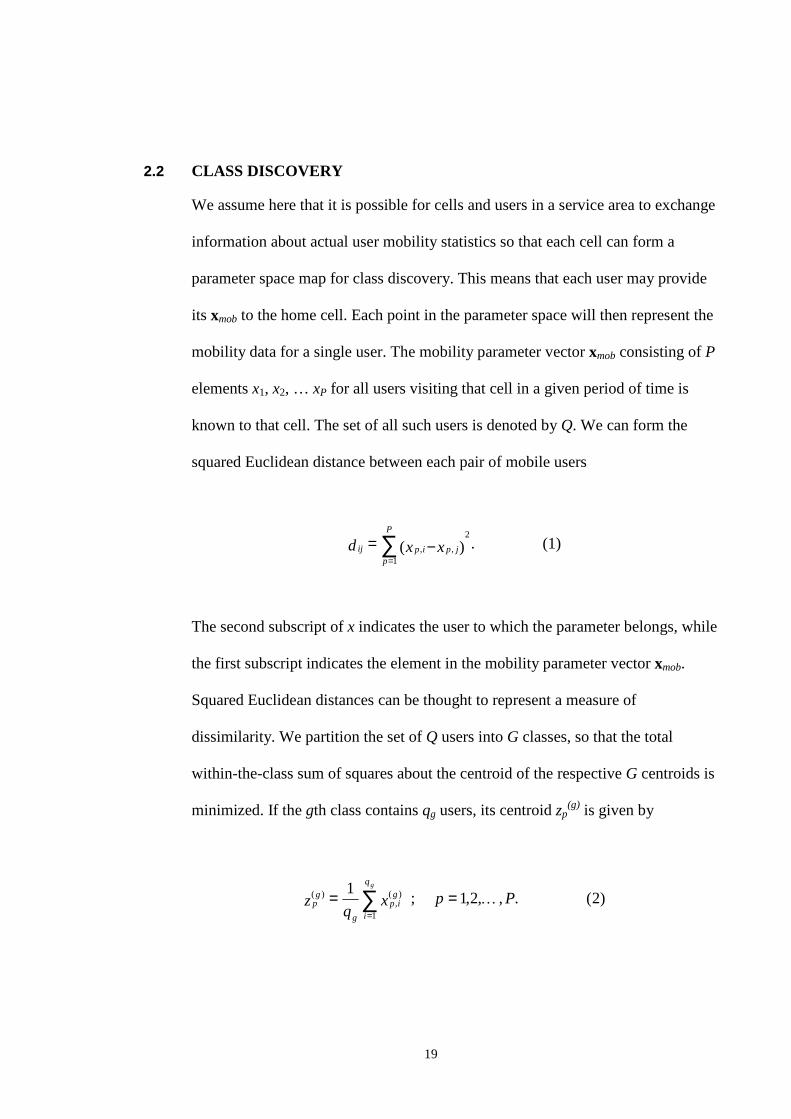
We assume here that it is possible for cells and users in a service area to exchange
information about actual user mobili ty statistics so that each cell can form a
parameter space map for class discovery. This means that each user may provide
its xmob to the home cell . Each point in the parameter space will t hen represent the
mobili ty data for a single user. The mobili ty parameter vector xmob consisting of P
elements x1, x2, … xP for all users visiting that cell i n a given period of time is
known to that cell . The set of all such users is denoted by Q. We can form the
squared Euclidean distance between each pair of mobile users
(1).)(1
,,
2∑=
−=P
pjpipij xxd
The second subscript of x indicates the user to which the parameter belongs, while
the first subscript indicates the element in the mobili ty parameter vector xmob.
Squared Euclidean distances can be thought to represent a measure of
dissimilarity. We partition the set of Q users into G classes, so that the total
within-the-class sum of squares about the centroid of the respective G centroids is
minimized. If the gth class contains qg users, its centroid zp(g) is given by
)2(.,,2,1;1
1
)(,
)( Ppxq
zq
i
gip
g
gp
g
== ∑=
20
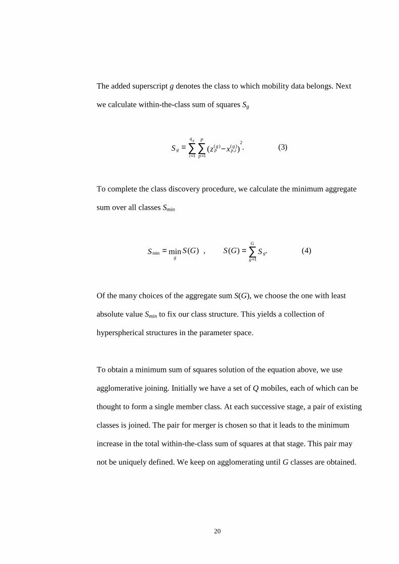
The added superscript g denotes the class to which mobility data belongs. Next
we calculate within-the-class sum of squares Sg
)3(.)(1 1
)(,
)(2∑∑
= =−=
q
i
P
p
gip
gpg
g
xzS
To complete the class discovery procedure, we calculate the minimum aggregate
sum over all classes Smin
)4(.)(,)(min1
min ∑=
==G
gg
gSGSGSS
Of the many choices of the aggregate sum S(G), we choose the one with least
absolute value Smin to fix our class structure. This yields a collection of
hyperspherical structures in the parameter space.
To obtain a minimum sum of squares solution of the equation above, we use
agglomerative joining. Initially we have a set of Q mobiles, each of which can be
thought to form a single member class. At each successive stage, a pair of existing
classes is joined. The pair for merger is chosen so that it leads to the minimum
increase in the total within-the-class sum of squares at that stage. This pair may
not be uniquely defined. We keep on agglomerating until G classes are obtained.
21
Alternately, we define h as being the class threshold and an h-procedure. Users
are added to a class until h ≥ dij is reached for within-the-class mobiles. In this
case, for all members of the class, we have dij ≤ h ∀ i, j. We can control class
density by choosing smaller values of h. The agglomeration method for class
discovery given above can be further quantified in terms of when and how to join
two groups. Figure 3 gives a segment of pseudo-code for the h-procedure
explained above.

22
Figure 3: Pseudo-code for class discovery using h-procedure.
Procedure ClassDiscovery: h-procedure
Given: num_Users, xmob for each user, threshold, iterationsnum_Not_Combined = num_Userscount = 1do
class_Threshold = threshold * count/iterationsfor i = 1 to num_Users
i++if i not marked
for j = i to num_Users
calculate dij
if dij < class_Thresholdagglomerate i and jmark jnum_Not_Combined--j++
count++num_Users = num_Not_Combined
while class_Threshold < thresholdnum_Classes = num_Not_Combined
Return: num_Classes

23
2.3 CLASS SPECIFICATION
Class discovery is easily followed by class specification. As explained later, we
need prior information for user mobility classification. This prior information
comprises of class prior probability, the mean values of user mobility parameters
and their covariances. The procedure described above is meant to provide the
number of classes from the collection of user parameter vectors and the mean and
covariance matrices can be calculated from class members once class
identification has been undertaken. Class specification also comprises calculation
of class characteristics, which are later assigned uniformly to all component
members.
To calculate class prior probabilities empirically, we proceed as below
)5(.q
q
T
gg =π
In (5), πg is the prior membership probability of a class g, qg is the number of
mobile users that were contained within class g and qT is the total number of
mobiles that were used in the class discovery procedure. For this expression to
become exact qT →∞, but (5) remains a good approximation as long as qT is a
large number. Let us also modify our notation slightly. We want to calculate the
class mobility parameter vector xmob(g), from individual class members which
furnish us with their mobility parameter vectors xmob,i. If xmob(g) is the mean class

24
parameter vector, meaning that it represents the average characteristics of the
class, an empirical expression for calculating xmob(g) can be written as
)6(.1
1,
)( ∑=
=q
iimob
g
gmob
g
qxx
The class mobili ty parameter vector can also assume the worst case characteristics
of that class. Worst case is defined here as the parameter value that leads to
maximum resource reservation. The choice of worst case value (min, max etc.)
depends on the physical definition of the parameter. We define ‘wcv’ – worst case
value operator - that selects the worst case value from a range. Then the class
mobili ty parameter vector is given by the expression of (7)
)7(.wcv ,1
)(xx imob
q
i
gmob
g
==
Finally, xmob(g) obtained from the expression (6) also gives the empirical class
mean vector µµg for class g. A PxP class covariance matrix ΣΣg for class g and xmob
= [x1 x2 … xP] is shown below
)8(.
222
222
222
21
22212
12111
=
σσσ
σσσσσσ
xxxxxx
xxxxxx
xxxxxx
g
PPPP
P
P

25
This is a symmetric matrix, where σ2x1x2 is equal to σ2
x2x1 etc., σ2x1x1 is the auto-
covariance of parameter x1 and σ2x1x2 is cross-covariance of parameter x1 with
parameter x2. An empirical estimate of these auto and cross covariances for class
g can be obtained from (9)
)9(.)]()([1
)(1
)()(,
1
)(1
)(,1
2
1
)()(,
22
1µµσ
µσ
gp
gip
q
i
ggi
g
xx
q
i
gp
gip
g
xx
xxq
xq
g
p
g
pp
−=
=
∑ −
∑ −
=
=
In this expression, xp,i(g) stands for the ith sample of the pth parameter in class g
and µp(g) denotes the mean obtained from qg samples of the pth parameter in class
g. Actually, the class mean vector is µµg = [µ1(g) µ2
(g) … µP(g)].

26
2.4 USER CLASSIFICATION
With the class discovery and specification done, we now proceed to the problem
of classifying an individual user given that we are presented the mobili ty
parameter vector xmob of that user. Assume that we have established the presence
of G classes. We define ζζ as a G-dimensional vector with zero-one indicators
designating the class membership of the user. For instance, if the user belongs to
class g, all but ζg member of the ζζ vector are zero. After establishing G classes,
we also define ππ as a G-dimensional vector of prior class probabilities π1, π2, …,
πG with the normalization condition π1+π2+…+ πG = 1. Prior probabili ty of class
membership indicates the known proportion of the users of each class in a mixture
of classes in a class id set ΓΓ. If the class-conditional probability density function
of xmob in a class with id Γg is given by pg(xmob), then the pdf of xmob in ΓΓ is given
by
)10(.)()(1
xx mobg
G
ggmobx pp ∑
=
= π
Given that the user submits xmob as its parameter vector, the aposteriori
probability ρg(xmob) that the entity belongs to the class with id Γg is given by
)11(.)(
)(
|1Pr
|Pr)(
x
x
x
xx
mobx
mobgg
mobg
mobgmobg
p
p
user
π
ζ
ρ
=
==
Γ∈=
27
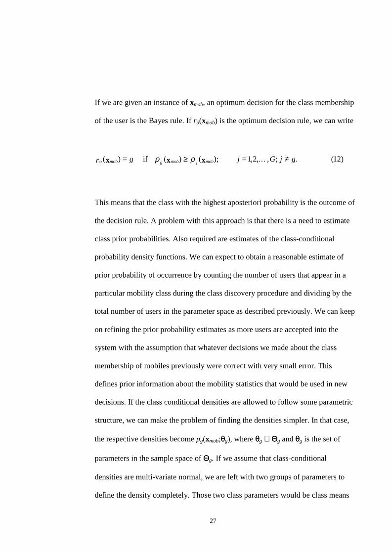
If we are given an instance of xmob, an optimum decision for the class membership
of the user is the Bayes rule. If ro(xmob) is the optimum decision rule, we can write
)12(.;,,2,1);()(if)( gjGjgr mobjmobgmobo ≠=≥= xxx ρρ
This means that the class with the highest aposteriori probability is the outcome of
the decision rule. A problem with this approach is that there is a need to estimate
class prior probabilities. Also required are estimates of the class-conditional
probability density functions. We can expect to obtain a reasonable estimate of
prior probability of occurrence by counting the number of users that appear in a
particular mobility class during the class discovery procedure and dividing by the
total number of users in the parameter space as described previously. We can keep
on refining the prior probability estimates as more users are accepted into the
system with the assumption that whatever decisions we made about the class
membership of mobiles previously were correct with very small error. This
defines prior information about the mobility statistics that would be used in new
decisions. If the class conditional densities are allowed to follow some parametric
structure, we can make the problem of finding the densities simpler. In that case,
the respective densities become pg(xmob;θθg), where θθg ∈ ΘΘg and θθg is the set of
parameters in the sample space of ΘΘg. If we assume that class-conditional
densities are multi-variate normal, we are left with two groups of parameters to
define the density completely. Those two class parameters would be class means
28
and class covariances. Prior information used to determine mobili ty class
membership of a user then consists of class prior probabiliti es and also the
estimated or measured values of conditional probabili ty parameters. Thus, we
define prior information matrix ΨΨ=(ππT,θθT)T. With the multi -variate normal
distribution of class parameters, i.e., xmob ∼ N(µµg, ΣΣg) for g=1, 2,…, G, where µµg
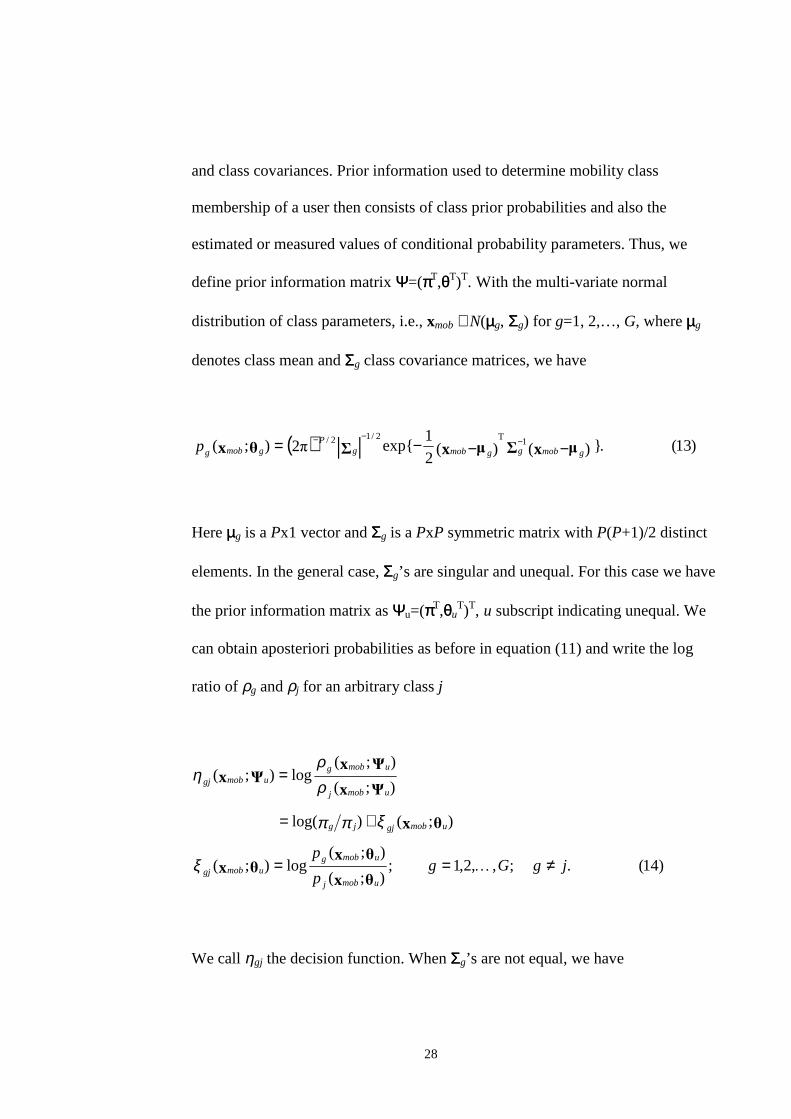
denotes class mean and ΣΣg class covariance matrices, we have
( ) )13(.)()(2
1exp2);( 1T2/12/ || xxx gmobggmobg
Pgmobgp −−−= −−−
Here µµg is a Px1 vector and ΣΣg is a PxP symmetric matrix with P(P+1)/2 distinct
elements. In the general case, ΣΣg’s are singular and unequal. For this case we have
the prior information matrix as ΨΨu=(ππT,θθuT)T, u subscript indicating unequal. We
can obtain aposteriori probabiliti es as before in equation (11) and write the log
ratio of ρg and ρj for an arbitrary class j
)14(.;,,2,1;);(
);(log);(
);()log(
);(
);(log);(
jgGgp
p
umobj
umobgumobgj
umobgjjg
umobj
umobgumobgj
≠==
+=
=
x
xx
x
x
xx
ξ
ξππ
ρρ
η
We call ηgj the decision function. When ΣΣg’s are not equal, we have

29
)15(.||
||log
2
1)()(
)()(2
1);(
1T
1T
xx
xxx
j
g
jmobjjmob
gmobggmobumobgj
−−−
−−−−=
−
−ξ
If we plot ξgj in the parameter space, it defines a hypershperical surface and we
call it quadratic classifier. The optimal Bayes rule ro(xmob) given above then
assigns a mobile with parameter vector xmob to the class with id Γg if
)16(.;,,2,10);( jgGgumobgj ≠=≤ xη
Otherwise, a class with id Γk is assigned if
)17(.;,,2,1);();( gkGkumobkjumobgj ≠=≤ xx ηη
Now consider the case in which class covariance matrices are all the same
(ΣΣ1,ΣΣ2,…,ΣΣg =ΣΣ). This results in substantial simpli fication in the classifier
expression of (15), since terms like xTmobΣΣg
-1xmob are the same for all classes and
cancel out in pair ratios. Equali ty of covariance matrices is indicated by the
subscript e in the expression that follows

30
)18( .;,,2,1
;)-()-(2
1);(
);()log(
);(
);(log);(
1T
jgGg
- jgjgmobemobgj
emobgjjg
emobj
emobgumobgj
≠=
=
+=
=
−
xx
x
x
xx
ξ
ξππ
ρρ
η
We obtain a set of linear equations in x1, x2,…, xP. Clearly when plotted in the
parameter space, this yields linear surfaces, hence we call this a linear classifier.
The linear optimal decision rule is also given by equations (16) and (17). In [21],
it has been shown that a multi -variate normal assumption on class parameter
distribution can yield satisfactory classifier performance even if the data is only
semi-normal or even non-Gaussian.
In order to assign a mobili ty class to a user, we must have the mobili ty parameter
vector xmob of that user. We assume that xmob has multi -variate normal
distribution. We make an arbitrary class g with id Γg as the base class. Starting
with the first mobili ty class, we calculate the decision function ηgj using either the
quadratic classifier of (15) or the linear classifier of (18). The choice of quadratic
or linear classifier should be governed by computational resources available and
required accuracy of classification decisions. Finally, the decision to assign a
class to a user is made by using the expressions of (16) and (17) and the decision
functions obtained above.
31
2.5 MOBILITY CLASSIFICATION ALGORITHM
The class discovery and specification procedure needs to be invoked periodically
to account for any time-dependent nature of user mobility. Also, the procedure
should be invoked separately in every cell since mobility is also spatially
dependent and we cannot expect the class structure discovered in one cell to hold
in another distant or near cell. Cells need to maintain mobility data of the users
who have recently visited the cell. This can happen by direct measurement, or
alternatively users can supply their mobility parameter vectors and the cell can
cache the vectors for later use, discarding them after a certain time period.
Mobility characteristics of a class have a much greater time period than the
mobility characteristics of a single user in a cell. Class discovery and specification
procedures need to be executed only once per several executions of the admission
control algorithm. As soon as a new user enters a cell, either through handoff
from another cell or by a new call request, that user communicates its mobility
parameter vector to the cell. A decision can then be made about the class of the
user by utilizing the rules given in equation (16) or (17). Either the linear or
quadratic classifier can be used, depending on how much processing demand can
be met and what kind of accuracy is desired. If the cost/time constraints call for
quick classification decisions, we can use the decision tree approach given above.
Whereas, our formal approach is expected to yield tight and efficient classes, a
decision tree would not take advantage of the clustering and class statistics. Thus,
in the general case, the decision tree approach will produce a larger number of
32
classes. Since our admission control procedure does aggregation separately for
different mobility classes, a larger number of classes leads to greater computation
in the resource and admission algorithms. Another fact that favors our formal
approach is that the decision-tree method does not discover and enforce the
natural class structure. It partitions the parameter space blindly. Thus, users
falling naturally in one class may get divided into separate and different classes
and users belonging to different classes may get lumped into one class. This
means that class specification becomes inaccurate, i.e., one which does not truly
represent user mobility. Finally, due to the sparseness at many leaves of the
decision tree, we might not have enough data to accurately determine class
characteristics.
How often it is required to run the class discovery and specification procedure
depends on the local conditions in a cell. A complete sketch of the mobility
classification algorithm is given below.
When determining worst-case characterization of a user class, calculation of worst
case parameter values depends on the physical phenomenon captured by the
parameter. We will take up this topic further in the next section.

33
Figure 4: Pseudo-code for mobility classification algorithm.
Procedure MobilityClassification
Given: period, stack_Sizeuser_Stack = stack_Sizeadmission_Control_Cycles = 0enable interruptdo
interrupt if new_User
get new_User.Parameter_Vectorpush new_User.Parameter_Vector on User_Stackcall userClassificationset new_User.mobility_Classadmission_Control_Cycles++if admission_Control_Cycles = period
disable interruptadmission_Control_Cycles = 0call classDiscoverycall classSpecificationenable interrupt
while forever
class_Discovery Subroutineread user_Stackplot user_Stackrun external Procedure classDiscovery <refer Figure 3>set user_ClassesReturn: num_Classes
34
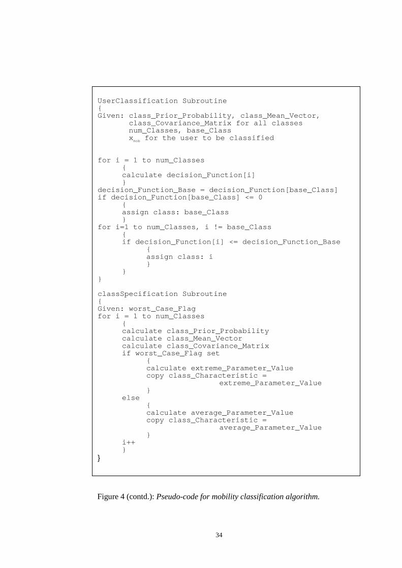
Figure 4 (contd.): Pseudo-code for mobility classification algorithm.
UserClassification SubroutineGiven: class_Prior_Probability, class_Mean_Vector, class_Covariance_Matrix for all classes num_Classes, base_Class x
mob for the user to be classified
for i = 1 to num_Classescalculate decision_Function[i]
decision_Function_Base = decision_Function[base_Class]if decision_Function[base_Class] <= 0
assign class: base_Class
for i=1 to num_Classes, i != base_Classif decision_Function[i] <= decision_Function_Base
assign class: i
classSpecification SubroutineGiven: worst_Case_Flagfor i = 1 to num_Classes
calculate class_Prior_Probabilitycalculate class_Mean_Vectorcalculate class_Covariance_Matrixif worst_Case_Flag set
calculate extreme_Parameter_Valuecopy class_Characteristic =
extreme_Parameter_Value
elsecalculate average_Parameter_Valuecopy class_Characteristic =
average_Parameter_Value
i++

35
2.6 SECTION SUMMARY
In this section, we have presented the steps to user mobili ty classification. The
first step is class discovery, where the mobili ty class structure in a cell i s
determined by using mobili ty parameter vectors xmob of users that may have
visited the cell i n a given period of time. The class discovery procedure we have
described yields a number of mobili ty classes with the class structure that
considers an expected clustering of mobili ty parameters. Our class discovery
procedure gives the number of classes and the mobili ty parameter vectors within
each class. The class specification procedure then uses this information to specify
a class mobili ty parameter vector as well as prior class membership probabiliti es.
After the number of classes and the class specification of each class have been
determined for a cell , any user originating a call or handing off in that cell can be
assigned a mobili ty class. This is done using our user classification scheme. When
a new user enters a cell (either through handoff or new call origination), the user
communicates its mobilit y parameter vector xmob to the cell . The cell uses this
information along with class specification output in the user classification scheme
to determine the mobili ty class of the new user.
We also discussed our scheme’s properties in reference to a decision tree
approach. A decision tree approach would be easy to implement and is less costly
in terms of computation, but it would be less accurate in determining the class
structure in a cell . We showed that class assignment decision from a decision tree
would also be less efficient.
36
Finally, each cell maintains a cache of mobility parameter vectors of the users that
have visited the cell in the past. If a class discovery procedure has to run every 15
minutes for example, then the cell will use mobility parameter vectors from the
past few days to determine its classes. Cycles in user mobility must be considered
when performing class discovery. For instance, if the cell needs to determine the
class structure on Sunday 12 pm to 12:15 pm, it needs to pull the mobility data for
only the past few Sundays tagged with the same time.

37
3. MOBILITY SPATIAL FLOW FRAMEWORK
In this section, we introduce a spatial flow framework for estimating resources to
provide quali ty of service to users in a microcellular wireless multimedia system.
In the spatial flow framework, we take advantage of the mobili ty classification of
users to aggregate individual users of the same class into a classed spatial flow. A
spatial flow is a statistical entity representing bandwidth demand in a service area
produced by the space-time variations of user mobili ty. This aggregate bandwidth
is calculated as the sum of current bandwidth requirement of each user
constituting the spatial flow. Spatial flows can then be used to estimate required
resources and perform admission control of new calls.
A spatial flow can be defined in terms of its space-time characteristics, such as its
speed and direction. However, in the particular case of spatial flows composed
from mobile users, it is necessary that the aggregate spatial flows represent the
mobili ty behavior of the users. Since we can measure each individual user's
mobili ty and call time statistics, we can model spatial flows with similar
characteristics. A spatial flow is then characterized by the average or worst-case
representation of its composing user's mobili ty statistics. Each classed spatial flow
has a class mobility parameter vector associated with it. This vector specifies the
transport process of the flow. A flow time statistics vector may also be required to
specify the dissipation and/or generation processes on the flow. Spatial flows are
divisible entities. We can predict the direction and strength of diversions of the
original spatial flow. These diversions of the root spatial flow are called
38
branching flows. We can track the behavior of root and branching spatial flows by
using the statistical characterization of the root flow.
We distinguish between three types of flows, depending on the presence or
absence of a dissipation and/or generation process. We use the term Conservative
Flow for a spatial flow, which does not change in quantity (bandwidth demand)
while traveling from a cell to another cell, only a transport process is present. A
Dissipative Flow, on the other hand, can dissipate while in transit, i.e., it can
decrease in quantity with time, but it cannot increase (transport and dissipation
processes only). We define a Generative-Dissipative Flow, a flow that can grow
or shrink with time depending on the statistics of its mobility and time data. For
conciseness, we denote the three types of classed spatial flows as C-flow, D-flow
and GD-flow.
A classed spatial flow takes on the mobility characteristics associated with a
particular class. For instance, consider a simplified example of 10 users belonging
to a class with class id Γg with the mobility parameter vector given by xmob(g) and
each user demanding a constant 30 kbps bit-rate channel. In this case, a flow with
an aggregate bit-rate of 300 kbps can be formed with the mobility characteristics
given by xmob(g). Only call time statistics of the aggregate spatial flow need to be
stated to complete the specification of the flow. We shall show how to accomplish
that later in this section.
39
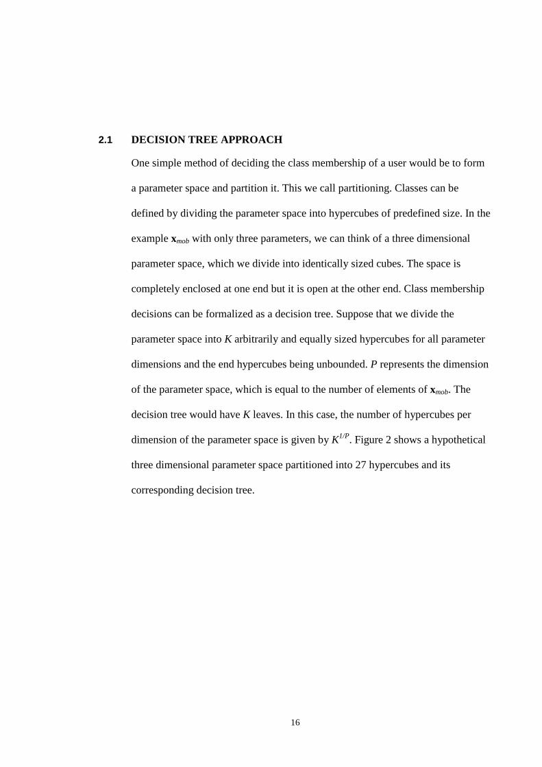
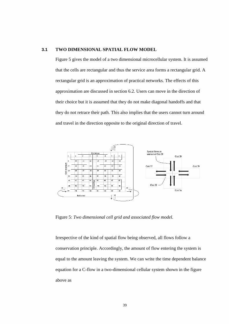
3.1 TWO DIMENSIONAL SPATIAL FLOW MODEL
Figure 5 gives the model of a two dimensional microcellular system. It is assumed
that the cells are rectangular and thus the service area forms a rectangular grid. A
rectangular grid is an approximation of practical networks. The effects of this
approximation are discussed in section 6.2. Users can move in the direction of
their choice but it is assumed that they do not make diagonal handoffs and that
they do not retrace their path. This also implies that the users cannot turn around
and travel in the direction opposite to the original direction of travel.
Figure 5: Two dimensional cell grid and associated flow model.
Irrespective of the kind of spatial flow being observed, all flows follow a
conservation principle. Accordingly, the amount of flow entering the system is
equal to the amount leaving the system. We can write the time dependent balance
equation for a C-flow in a two-dimensional cellular system shown in the figure
above as
40
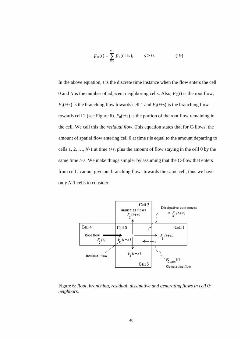
)19(.0);()(1
00 ≥+= ∑
−
=
sstFtFN
ii
In the above equation, t is the discrete time instance when the flow enters the cell
0 and N is the number of adjacent neighboring cells. Also, F0(t) is the root flow,
F1(t+s) is the branching flow towards cell 1 and F2(t+s) is the branching flow
towards cell 2 (see Figure 6). F0(t+s) is the portion of the root flow remaining in
the cell . We call this the residual flow. This equation states that for C-flows, the
amount of spatial flow entering cell 0 at time t is equal to the amount departing to
cells 1, 2, …, N-1 at time t+s, plus the amount of f low staying in the cell 0 by the
same time t+s. We make things simpler by assuming that the C-flow that enters
from cell i cannot give out branching flows towards the same cell , thus we have
only N-1 cells to consider.
Figure 6: Root, branching, residual, dissipative and generating flows in cell 0/neighbors.

41
Equation (19) and the cell designation represent a general case where the cell of
interest is designated as cell 0. Neighbor cells for which branching flows have to
be determined should be designated as shown in Figure 6. Since N=4 for this
model, we do not include the branching flow towards cell 4. Note that the
definition of the spatial flow is general, since we say nothing about the initial
conditions when we obtain F0.
For a D-flow there is an added term indicating the amount of flow (bandwidth
demand) that dissipates as the flow moves through the cell
)20(.0);()()(1
00 ≥+++= ∑
−
=
sstFstFtFN
iid
We consider two stages of a GD-flow. The first stage is that of generative
aggregation when new users admitted into the cell become parts of the spatial
flow. In the second stage, the aggregation process is stopped and the flow
dynamics become essentially those of a D-flow
)b21(.);()()(
)a21(0);()()(
0,0
0,0
ssstFstFstF
ssstFstFstF
gen
N
iidgengen
gen
N
iidgen
>+++=+
≤≤+++=+
∑
∑
=
=
The two parts of equation (21) indicate the generative aggregation-transport and
dissipative-transport processes. Note that in this equation, the generation process

42
continues from time t up to a fixed time t+sgen, after which it is assumed to
terminate and then only the dissipative-transport processes continues. F0,gen grows
with time; its growth rate determined by the call arrival intensity, bandwidth
demand, current traffic load in the cell and the admission control algorithm.
Equations (19), (20) and (21) are called the balance equations for C, D and GD
type flows respectively.
Let there be qg mobile users comprising the classed spatial flow, each demanding
a fixed bandwidth Cu,g. If the flow enters a cell at time t, then the value of the root
spatial flow is determined from
)22(.)(1
,)(
0 ∑=
=q
ugu
gg
CtF
The subscript g indicates the class to which the flow belongs. Both time and
mobility statistics are required to describe a flow. We have already laid out the
procedures of classifying user mobility and forming class specification. A classed
spatial flow inherits the mobility class characteristics of the class it belongs to.
Time characteristics of a spatial flow are determined by the time statistics vector
Tft=[Mg Eg].
To proceed further, we give a few details of the members of spatial flow mobility
parameter and time statistic vectors. Time statistic is defined with two parameters,
mean component call duration Mg and mean component elapsed time Eg. We

43
assume that the time characteristics of individual users can be represented by a
known probabili ty distribution. Let this distribution be given by pu,g(t). If there are
qg users in a classed spatial flow, the time distribution of the flow is given by the
scaled convolution of component users' distributions
)23(.)()()(1
)( ,,2,)( tptptp
qtp gqggt
g
gft g
∗∗∗=
If the call holding time of component users follow an exponential distribution for
instance, the component call duration pft would have an Erlang-qg distribution.
From equation (23) and the statistical independence of pu,g's, we can write for the
mean of pft
)24(.1
1,∑
=
=q
ugu
g
g
g
mq
M
Mean call holding time of each individual component user is denoted by mu,g.
Similar comments apply to mean component elapsed time Eg, the time already
spent by users composing the flow in call holding state. The expression Eg=1/qg
Σu=1qg eu,g can be used to calculate Eg. Here eu,g represents the elapsed time of the
user u comprising the flow with class g.

44
Next we consider the parameters of user mobili ty. The first set of parameters is
related to the time spent by a user in a cell – the cell residence time. We assume
that the cell residence time of a user follows a known distribution, which can be
defined by two parameters. For example, if this distribution is a generalized
gamma distribution [14], we need a shape and a scale parameter. Because we can
easily translate the first and second moment of cell residence time to the above
distribution parameters, we can use mean and variance values in the mobilit y
parameter vector. Measuring and calculating means and variances is much
simpler and also independent of the distribution form. The remaining parameters
are concerned with defining to which cell the user is expected to handoff . They
are handoff probabilities for the neighboring cells. In our model of the rectangular
grid, path retracing and diagonal handoffs are not allowed. We need to consider
three handoff parameters; the handoff probabili ty for the fourth cell i s always zero
for D-flows and therefore not needed. For GD-flows, that probabili ty can be
calculated from the normalization condition
)25(.14,3,2,1, =+++ PPPP HHHH
PH,i is the handoff probabili ty to cell i (refer to figure 6). For a C-flow in figure 6,
we can write the following equations for the classed branching flows with the root
flow in cell 0 and the branching flows directed towards cell 1, 2 and 3
)26(.3,2,1);()()()( )(0,
)(,
)( ==+ itFsPtPstF ggR
giH
gi

45
The expression (26) warrants some explanation. The superscript g has been
introduced for the handoff probabili ty to indicate the class of the mobili ty
parameter vector xmob(g) of the classed C-flow. Also in this expression, t is the
time the C-flow is admitted in the cell , PR,g is the cumulative probabili ty of the C-
flow cell residence time, s is some future time instant of interest and Fi(g)(t+s) are
the branching flows (after s seconds have passed) of the root flow F0(g)(t) that had
entered cell 0 at time t. Note that cumulative probabili ty is a non-decreasing
function of the time s. As s increases PR,g may increase too.Also, since PR,g of a
C-flow is calculated from xmob of individual users, it is a function of time as well
as the current cell . PH,i(g) is a function of time too, but since the mobili ty
parameter vectors of all classes in a cell are updated much less frequently, PH,i(g)
will remain constant for the li fetime of the C-flow. This means that the branching
flows Fi(g)’s continue to grow until the time when the root flow ceases to exist in
cell 0. This time, we call the flow lifetime, Tlife. Thus when s= Tlife, we have
)27(.)()()()](max[ )(0
)(,
)()()( tFtPTtFstF ggiH
glife
gi
gi =+=+
In (27) the superscript g on Tlife indicates the class of the C-flow. Flow cell
residence time distribution may have a long tail and so the condition for obtaining
the maximum value of the branching flows in (27) may never be met. We relax
the definition of Tlife by defining it to be the time s when s→Tlife if PR,g→1.

46
Lemma 1:
Flow lifetime of a C-flow is proportional to its cell residence time statistics. This
can be shown by computing the residual flow F0(g)(t+s), residual flow being the
amount of the root C-flow still left in cell 0 after passage of a certain time s.
Using the balance equation of (19) and the branching flows of (26), we obtain the
residual flow
)28(.)()]()()()(1[)( )(0,
)(3,
)(2,
)(1,
)(0 tFsPtPtPtPstF g
gRg
Hg
Hg
Hg ++−=+
Using the normalization condition of (25) for handoff probabilities with PH,4(g)
being zero, (28) can be simplified to
)29(.)()](1[)( )(0,
)(0 tFsPstF g
gRg −=+
Residual flow diminishes as the PR,g term in (29) approaches unity. Time taken by
the residual flow to disappear is actually the flow lifetime. To calculate this, we
proceed as follows
)30(.Pr
0;1Pr
1Pr)(
,
,
,,
ε
εε
=>⇒
→−=≤⇒
→≤=
sT
sT
sTsP
maxgR
maxgR
maxgRmaxgR

47
In the above equation, TR,g is the random variable representing cell residence time
of the C-flow. Using Chernoff’ s bound, we can obtain an upper limit on the value
of smax
)31(.)(
ln1
exp)(minPr
|,
,,
ετττ
τ
τ
min
max
Ts
TsT
gR
min
max
sgRmaxgR
=
−
Ω≈∴
Ω=>
In the expression of (31), Ω(TR,g) is the moment generating function of TR,g given
by E[exp-τTR,g] and τ, τmin represent the dummy variables for forming and
evaluating the moment generating function. Since in this case smax = Tlife, from
equation (31) it can clearly be seen that the C-flow li fetime is in direct proportion
to its cell residence time statistics.
Also note that in equation (31), there is a tunable parameter ε. If the C-flow has
diminished with 95% confidence, the value of ε should be less than 0.05. Smaller
values may be more accurate, but they have the effect of stretching the C-flow
lifetime beyond its useful range. Flow lifetimes will be useful later when we track
individual classed spatial flows to estimate required resources. A flow would be
tracked for the duration of its lifetime after which it would be assumed to have
diminished completely.

48
We now turn to D-flows. Since the flow dissipates in addition to transportation,
we also have an active dissipation component. Branching flows for D type classed
spatial flows can be calculated from
)32(.3,2,1);()](1)[()()( )(0,,
)(,
)( =+−=+ itFEsPsPtPstF gggLgR
giH
gi
Here PL,g represents the cumulative probability of flow component call duration.
PL,g is also a non-decreasing function of s, so the term 1- PL,g shrinks with time.
Inclusion of the component elapsed time variable Eg ensures that we account for
time already spent by users in the call holding (busy) state before becoming a part
of the new D-flow. This way we need not consider as the probability of
dissipation in cell 0 - the probability of the D-flow dissipating in cell 0 due to call
completions. Also, PR,G and PL,G are the space-time dependent properties of a D-
flow and are calculated from xmob of individual users. The dissipative component
of the D-flow Fd is the disappearing part of the D-flow (due to call terminations)
)33(.,0
;),()()(
)(0,
)( Ts
TstFEsPstF
life
lifeg
ggLg
d >
≤+=+
The D-flow will diminish to become very small after Tlife, so for s> Tlife there is no
need to keep track of Fd.
49
Lemma 2:
The li fetime of a D-flow is proportional to flow cell residence as wells as flow
component call duration statistics. To confirm this statement, we proceed as
before for C-flows. We calculate the residual flow F0(g)(t+s) from the branching
flows of (32) and the dissipative component of (33), using the balance equation of
(20) and the handoff probabili ty normalization condition of (25)
)34(.3,2,1);()](1)][(1[)( )(0,,
)(0 =+−−=+ itFEsPsPstF g
ggLgRg
It is clear from the expression of (34) that the residual flow diminishes when
)35(.PrPr 2,1, ε≈>> sTsT gLgR
Here TL,g is the random variable representing flow component call duration. A
conservative estimate of the D-flow li fetime is obtained by using Chernoff’ s
bound on the tail of cell residence time and component call duration distributions
separately
)36(.),min(
)(expln
1
)(ln
1
21
,
2
2
,
1
1
|
|
2
2
1
sss
Ts
Ts
max
gLE
gR
g
=
Ω≈
Ω≈
=
−
=
ετ
ετ
ττ
τ
ττ

50
In equation (36), Ω(TL,g) is the moment generating function of component call
duration, s1, s2 are the maximum values of time obtained by Chernoff’ s bound on
the tail of cell residence time and flow call duration distributions, respectively,
and τ1, τ2 are dummy variables. Since smax= Tlife, from the expression of (36) it is
obvious that the D-flow li fetime is proportional to both its cell residence and
component call duration statistics.
The estimate of f low li fetime obtained above for D-flows is generally very
conservative. Equation (36) implies that a D-flow may vanish from a cell either
by dissipating completely or by branching out into the neighboring cells. In
actuali ty, the component call duration factor in (34) should expedite the decay of
residual flows. We can expect the residual of a D-flow to diminish earlier than the
residual of an equivalent C-flow. When estimating the D-flow li fetime, it is better
to use (34) and to consider the value of both residence and component call
duration cumulative probabili ty. If the functional form of f low cell residence and
component call duration distributions is known, we can make fairly accurate
predictions of the flow li fetime without evaluating the complex expressions of
(31) and (36). For instance, if we knew that the cell residence time is Gaussian,
we can estimate the spatial C-flow li fetime easily by knowledge of the mean and
standard deviation of cell residence time.

51
Next we turn our attention to GD-flows. As we mentioned earlier, there is an
initial generative-aggregation phase for GD-flows. The amount of aggregation
achieved depends on the call traffic intensity, bandwidth demand and admission
control of new users. For simpler case, let us first assume that our cells can
measure call arrival rate on admitted calls. From the bandwidth requirement of
each call, we can derive the overall bandwidth demand. We denote the
instantaneous, time varying, admission control modified call arrival rate by λg(t)
and bandwidth demand by Bg(t). Then the GD-flow accumulated in the interval [t,
t+sgen) is given by
)37(.)()()()(
,0yBystF g
st
tyggen
g
gen
gen
∑+
=
=+ λ
We will not further pursue the mechanics of accumulation of a GD-flow. For now
we concentrate on the statistical time dynamics equations for a GD-flow. If sgen is
much smaller than flow mean cell residence time and mean component call
duration minus component elapsed time, then we can approximate the flow
invocation time t to be equal to the time t+sgen. This implies that the degree of
generative-aggregation is much greater than the dissipation and transport
processes in the interval [t, t+sgen). After time t+sgen only dissipation and transport
processes continue. We can write equations for the four branching flows of a GD-
flow for our rectangular grid model. The equations are the same as for a D-flow.
The only difference is that a GD-flow can emanate branches in any direction since

52
it is generated internally in cell 0 and so is free to move towards any one of the
four neighboring cells
)38(.;4,3,2,1
);()](1)[()()( )(0,,
)(,
)(
ssi
tFEsPsPtPstF
gen
gggLgR
giH
gi
>∀=
+−=+
If the sgen is very small, it would be safe to assume that Eg=0. However, we keep
the component elapsed time for now. In that case, the expressions for the GD-
flow lifetime Tlife would be identical to those for D-flows with the additional
condition of s>sgen.
If the two dimensional service area model is different from the one given in
Figure 5, there may be more or less branching flows then those given in
(19/20/21). For instance in a hexagonal cell array, a D-flow can have five
branching flows. In that case, we need to change the value of N in (20). We would
also need to change the number of parameters in the mobility parameter vector
xmob so as to accommodate handoff probability for a greater or fewer number of
cells.

53
3.2 ONE DIMENSIONAL FLOW MODEL
The one dimensional flow model is a simplification of the previously discussed
two dimensional model. This model can be useful in specific situations such as
representing service areas on roadways. From Figure 7 below, we can write the
balance equation for spatial flow in cell 0
)39(.)()()()()()(
2
)(
1
)(
0
)()(
0stFstFstFstFtF
gggg
d
g +++++++=
For C-flows the dissipative component Fd of the root flow is zero. For C-flows as
well as for the D-flows, we can ignore the first or the second branching flow F1 or
F2, depending on the cell from which the flow initially handed off into cell 0. For
example, if the flow enters cell 0 from cell 2, we can ignore the F2 branching flow
since we assume that the users do not retrace their path of travel. For GD-flows,
we force the condition s>sgen for the transport process after flow aggregation, in
the same way as for two dimensional GD-flows.
Figure 7: One dimensional service area model with spatial flows.

54
Vectors describing a one dimensional spatial flow are the same as those defining a
two dimensional flow, with the difference that instead of defining four or more
different handoff probability terms, we need to now define only two.
Additionally, we may ignore the ith handoff probability of a D-flow coming from
cell i. Branching flows and flow lifetime may also be computed in a way similar
to the two-dimensional flow model.
Flows are cell-based entities whose existence is limited to their home cell. They
either originate in a cell or are handed off from a neighboring cell. A spatial flow
vanishes when all the composing users terminate their calls or handoff into
neighboring cells. We form branching flows in the first tier immediate neighbors
only and not into second and third tier neighbors. After the spatial flow vanishes,
it looses its existence and new flows have to be formed by the users composing
the original flow. There is a reason for forming branching flows for the first tier
neighbors only. We need resource estimation for immediately adjacent cells, as
would be seen in the next section. We have observed in our experiments with the
algorithm of [19] that reservations in second and third tier cells are very small and
can therefore be ignored easily without effecting performance. The little
additional accuracy gained by reservations in far off neighbors costs a lot in terms
of algorithm complexity and computation overhead. Complexity arises by
extending branching flows, which generally increase by a factor of N (number of
neighboring cells) with every additional tier of cells. The accuracy obtained is
55
little compared to the extra effort required to track all the branching flows,
computing and maintaining them.
The spatial flow model supports the space-dependent heterogeneous nature of
user mobility. This is accomplished by maintaining local statistics of mobility and
using those statistics when forming classed flows. The spatial flow framework we
have given is in fact independent of any assumptions about user mobility. We can
revert to spatially homogeneous characterization of mobility and use virtually the
same equations for spatial flows in that case too. We need only to change the way
we perceive and measure user mobility characteristics.
56
3.3 SECTION SUMMARY
In this section, we have laid out a classed spatial flow framework for tracking user
motion in the service area. We have presented the statistical time dynamics
equations for three types of flows, C-flows, D-flows and GD-flows. In the
following sections, we will employ the D-flows to track handoff calls and GD-
flows to track new call originations. The same flow framework will also be
employed in resource reservation for future handoffs and admission control for
newly originated calls in the wireless cellular network. We have also given the
expressions for calculating the lifetime of classed spatial flows. If the lifetime of a
flow is known, it needs to be tracked only up to the time when it expires, i.e., the
time when flow lifetime is reached. In summary the different flows composed
from mobile users are as follows.
• A C-flow is a spatial flow which conserves itself as it moves from cell to cell.
It is formed by users in motion but maintaining calls indefinately. Clearly, a
C-flow is not very useful but it nevertheless helps in developing ideas for
other flow types.
• A D-flow can dissipate as it moves from cell to cell. It is formed in a cell by
users who have originated their calls in another cell but are trying to handoff
in a particular cell. D-flows are useful in tracking handoff users.
• A GD-flow can generate and dissipate as it moves out of a cell. It is formed by
users originating new calls in a cell. A GD-flow models traffic generation in
the system. It is also used to perform admission control as shown in section 4.

57
4. QUALITY OF SERVICE WITH SPATIAL FLOWS
We can use the flow framework presented in the last section to provide cell level
quality-of-service, QoS, as determined by (Pdrop, Pblock). We do not provide
explicit expressions for call dropping probability. Instead our approach is to give
expressions for estimating required resources in neighboring cells and to perform
admission control to attain the minimum possible call dropping rate, constrained
by a given call blocking rate. We then conduct simulations that help us establish
experimentally which tunable variables should be adjusted to achieve the desired
quality of service (Pdrop, Pblock). With the blocking probability being the
constraining factor, we select a value of Pdrop from simulations that is low enough
and at the same time maintains the required blocking probability. A certain value
of the QoS doublet (Pdrop, Pblock) also fixes the range for cell resource utilization.
We will be able to evaluate the utilization vs. QoS tradeoff in Section 6. However,
it seems intuitive that a stringent requirement on Pdrop would decrease resource
utilization.
It is possible to derive expressions for QoS parameters (Pdrop, Pblock), as has been
done in [15] and [16], but approaches like those suffer from state-space explosion
due to the complexity of underlying problem. Our algorithm can be used
adaptively to control call dropping and blocking rate.
In a cellular system at any given time there may be several active users. For
resource reservation and admission control, users are handled through the D and

58
GD type flows they form. At any moment in time there may be several D or GD
type flows in a cell , each individual user being part of only one spatial flow. Thus,
space-time varying bandwidth demand can be accounted for.
We proceed by assuming that time advances in discrete intervals of duration δ
seconds. Our algorithm calculations is invoked synchronously at the end of each δ
seconds interval – the algorithm step size. We also assume existence of soft
handoff , i.e., the abili ty of a user to communicate with more than one base
stations before completing a full handoff after which the user may communicate
only with the base station of its home cell . This happens while the user is in the
transition region between cells where radio coverage of two or more cells
overlaps. This is necessary in our algorithm because there should be a suff icient
number of users in the transition region to form an aggregate spatial flow before
that flow can be accommodated in the destination cell . Due to this aggregate
nature of our algorithm it is more suitable for networks with a large number of
handoffs per unit time operating at full or near full capacity. With low traff ic
volume, the algorithm degenerates to a per-user scheme rather than aggregate,
since then most of the spatial flows are comprised of a single user. This is not
necessarily harmful because the increased amount of computation per user would
be incurred only under only low loads when it is not detrimental to performance,
while at high loading aggregation would increase and so the computation per user
would decrease significantly. In order to avoid complexities, we assume also that
the area of the transition region is much smaller than the overall cell area.

59
Next we present a handoff scheme which works with our resource reservation
algorithm. The description of the resource reservation algorithm is given next.
Then we explain our admission control algorithm.

60
4.1 HANDOFF SCHEME
With the framework of classed spatial flow in mind we continue with the handoff
scheme. Suppose that at time t, we have a classed flow F0(g,n) requiring handoff
into cell 0. We have made one addition to our notation for classed flows. A new
superscript n has been added to indicate the cell from which the new D-flow will
be handed off. Thus, the spatial flow F0(g,n) belongs to class g and is entering cell
0 from cell n. There are two mutually exclusive possibilities.
1. The cell has enough free resources (primarily free bandwidth) to admit the
flow. In that case all the users comprising the flow complete a successful
handoff and the cell enrolls a new D type spatial flow.
2. There are less than required resources (bandwidth) in cell 0. In that case, the
spatial flow cannot be admitted.
In the second case, a new classed spatial flow is formed by leaving off all the
users not having an urgent flag set. The users that do not have the urgent flag set
can be expected to maintain their existing call connections without getting
dropped. They will be considered for handoff in the next cycle of execution. We
let them stay in the transition region without performing a handoff so that they
could be considered in the next cycle of execution.
When a user enters a transition region initially, it requests a handoff with the new
destination cell. The destination cell estimates the position of the user in the

61
transition region between two cells and if the user is expected to leave the
influence of its old home cell, an urgent flag is set. Alternately, the mobile may
set the urgent flag itself by measuring received signal strength.
Figure 8: Users in transition region with urgent or non-urgent handoffs.
After the formation of the new classed spatial flow with all composing users
having the urgent flag set, we check for free resources in the destination cell. If
the destination cell has enough resources, we admit the classed spatial flow.
Finally, if there is a resource shortage, we drop users in order of most recently set
urgent flag. Repeated handoff admission retries are then executed with the
remaining users following the procedure outlined above.
All incoming flows are enrolled with the home cell. All spatial flows handing off
from the neighboring cells are D-flows. This means that handed off users are
tracked through the spatial flow framework only. New calls, if admitted, form
GD-flows and are tracked through their respective GD-flows. Only when handing

62
off to other cells do the individual users become visible again. The enrollment
procedure involves the following steps.
1. Determining and storing the class of a spatial flow. Assigning the flow its
xmob(g).
2. Calculating the time statistic vector of the flow Tft.
3. Calculating flow li fetime Tlife.
4. Assigning a classed flow unique id to differentiate this flow from other D-
flows in the cell . The unique id is released after the time Tlife.
Users only become individually visible to the algorithm at handoff or at admission
of a new call . When handing off , users are required to identify themselves and
transmit information about their mobili ty characteristics, time variables and
bandwidth requirements. The cell can then determine the user’s mobili ty class.
Cells are required to accept handoff users. On the other hand, new users are
admitted only if the admission test succeeds. If the cell has no extra capacity for a
handoff user and the urgent flag is set, the call for that user is dropped.
We give the handoff procedure pseudo-code below.
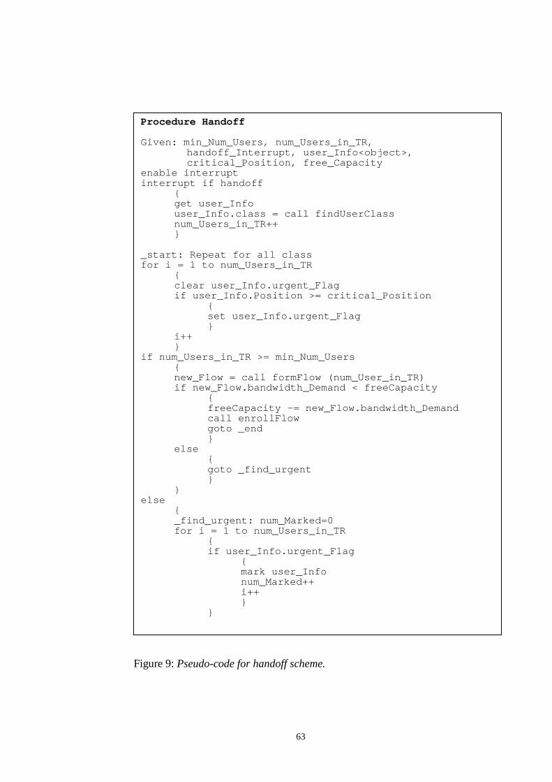
63
Figure 9: Pseudo-code for handoff scheme.
Procedure Handoff
Given: min_Num_Users, num_Users_in_TR,handoff_Interrupt, user_Info<object>,critical_Position, free_Capacity
enable interruptinterrupt if handoff
get user_Infouser_Info.class = call findUserClassnum_Users_in_TR++
_start: Repeat for all classfor i = 1 to num_Users_in_TR
clear user_Info.urgent_Flagif user_Info.Position >= critical_Position
set user_Info.urgent_Flag
i++
if num_Users_in_TR >= min_Num_Usersnew_Flow = call formFlow (num_User_in_TR)if new_Flow.bandwidth_Demand < freeCapacity
freeCapacity -= new_Flow.bandwidth_Demandcall enrollFlowgoto _end
elsegoto _find_urgent
else
_find_urgent: num_Marked=0for i = 1 to num_Users_in_TR
if user_Info.urgent_Flag
mark user_Infonum_Marked++i++

64
Figure 9 (contd.): Pseudo-code for handoff scheme.
_retry: new_FLow = call formFlow (num_Marked)if new_Flow.bandwidth_Demand < freeCapacity
freeCapacity -= new_Flow.bandwidth_Demandcall enrollFlowgoto _end
elsecall dropLatestUser (num_Marked)num_Marked—goto _retry
- end:
findUserClassSubroutine: Gives the mobility class of a user
enrollFlowSunroutine: Enrolls a flow in a cell
dropLatestUserSubroutine: Instructs the old cell to drop a
call from the user requesting handoff most recently

65
4.2 RESOURCE RESERVATION SCHEME
Suppose we have a spatial flow that has completed a handoff as a D-flow in cell
0. Let the flow be F0(g,n), meaning that it is a flow with mobili ty class g and it is
being handed off from neighboring cell n. With flow li fetime given by Tlife,φ
(subscript φ being a unique flow id), the number of times the reservation
algorithm need to be executed in all the neighboring cells for this flow is given by
)40(. ,
δφT
Nlife
a =
Here algorithm step size δ is the time interval defined previously. We have shown
that for the algorithm of [19], decreasing δ may improve algorithm performance
markedly.
The spatial flow that enters cell 0 from cell n would either dissipate or move to
other cells at some future time. To determine what quantity of the flow would
enter into each one of the neighboring cells, we use the statistical time dynamics
equations for branching flows of a D-flow. With these equations, we compute
Fi(g,n)(t+jδ) and Fd
(g,n)(t+jδ); i=1, 2, …, N-1; j=1, 2,…, Na, where N is the number
of neighboring cells. The results of the computation of branching flows and the
dissipative component are stored. Bandwidth needed in a neighboring cell at some
future time can now be calculated from the following expression

66
)41(. ,,2,1;0
; ))((
))(()(
),0,,(
),0,,(
),0,,(
,
NjN
NjtF
NjtFKjtR
arp
rpmng
i
rpmng
i
rg
mng
Di
=>
−+
−++⋅=+
=
==
δ
δδ
φ
φφ
The tunable parameter Nrp is a positive integer and can be used to adjust the
amount of reserved bandwidth in neighboring cells. Nrp.δ corresponds to the
Reservation Period. Krg is the reservation gain, which can also be used to tune the
reserved bandwidth up or down. In this regard, a control strategy can be adopted
whereby the handoff failure rate and call blocking rate can be used to control the
value of Krg and Nrp for desired values of Pdrop and Pblock. Ri,D(g,n,m,φ) is the reserved
capacity in cell i due to the spatial flow with flow id φ in cell m=0 being handed
off from cell n. The D subscript shows that the flow is dissipative and g is the
mobility class of the D type spatial flow. A unique id φ is assigned to the flows
since there may be more than one flow of the same description (i.e., having the
same values of g, i, n, m). Other conditions on (41) are as given in (42) below
)42(. 0))((,0for
)())((,for
))(())((
),,,(
),,,(),,,(
),,,(),,,(
=−+≤−
+=++≥+
−+>++
δ
δδ
δδ
φ
φφ
φφ
NjtFNj
NtFNjtFNNj
NjtFNjtF
rpmng
irp
amng
irpmng
iarp
rpmng
irpmng
i
Cell i calculates the gross reserved capacity Ri,D,gross(t+jδ) due to all the D type
flows in its neighbor cells from (43)
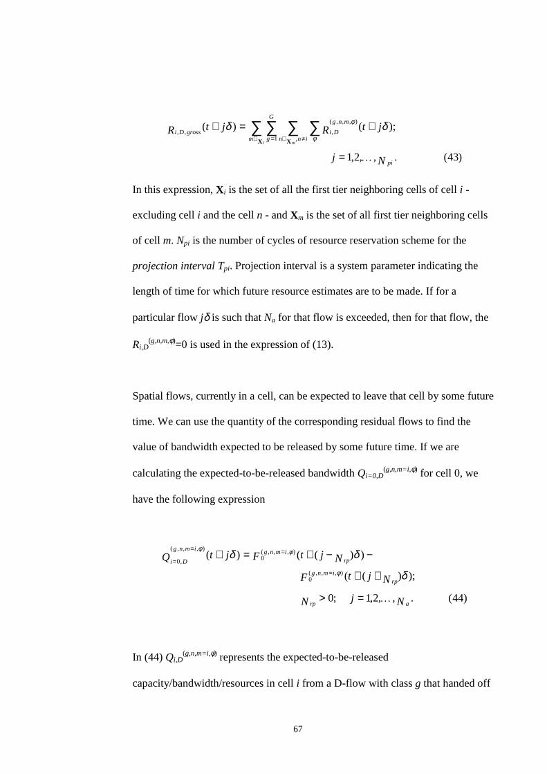
67
)43(. ,,2,1
);()(1 ,
),,,(
,,,
Nj
jtRjtR
pi
m
G
g inn
mng
DigrossDi
i m
=
+=+ ∑ ∑ ∑ ∑∈ = ≠∈X X φ
φ δδ
In this expression, Xi is the set of all the first tier neighboring cells of cell i -
excluding cell i and the cell n - and Xm is the set of all first tier neighboring cells
of cell m. Npi is the number of cycles of resource reservation scheme for the
projection interval Tpi. Projection interval is a system parameter indicating the
length of time for which future resource estimates are to be made. If for a
particular flow jδ is such that Na for that flow is exceeded, then for that flow, the
Ri,D(g,n,m,φ)=0 is used in the expression of (13).
Spatial flows, currently in a cell, can be expected to leave that cell by some future
time. We can use the quantity of the corresponding residual flows to find the
value of bandwidth expected to be released by some future time. If we are
calculating the expected-to-be-released bandwidth Qi=0,D(g,n,m=i,φ) for cell 0, we
have the following expression
)44(. ,,2,1;0
);)((
))(()(
),,,(0
),,,(0
),,,(
,0
NjN
NjtF
NjtFjtQ
arp
rpimng
rpimngimng
Di
=>
++
−−+=+=
==
=
δ
δδφ
φφ
In (44) Qi,D(g,n,m=i,φ) represents the expected-to-be-released
capacity/bandwidth/resources in cell i from a D-flow with class g that handed off

68
from the neighboring cell n and has a unique flow id φ. The following conditions
apply to Qi=0,D(g,n,m=i,φ)
)45(. 0))((,for
)())((,0for
))(())((
),,,(0
),,,(0
),,,(0
),,,(0
),,,(0
=++≥+
=−+≤−
++>−+
=
==
==
δ
δ
δδ
φ
φφ
φφ
NjtFNNj
tFNjtFNj
NjtFNjtF
rpimng
arp
imngrp
imngrp
rpimng
rpimng
Here t is the time when the spatial flow entered cell i=0 initially. To compute the
gross expected-to-be-released capacity Qi,D,gross by D-flows at one time in a cell i,
we sum over all the D type flows in the cell
)46(. ,,2,1;)()(1
),,,(
,,, NjjtQjtQ pi
G
g n
imng
DigrossDii
=+=+ ∑∑ ∑= ∈
=
φ
φδδ
X
For (46), we modify the definition of Xi. Xi is now a set of all the neighbors of
cell i. Any new call arrival and acceptance is modeled as a GD- flow. For a
generative-dissipative flow, we had previously defined an aggregation interval
sgen. The GD-flow builds up in this interval and after the generation process
terminates, it behaves just like a D-flow. We can form a different GD flow every
sgen seconds, depending on the intensity of traffic arrivals. Thus, at any given
time, there would be a stream of GD-flows within the cell. We can again use the
statistical time dynamics equations of GD-flows to find out the reservation in
neighboring cells. Bandwidth reservation expressions for GD-flows in cell 0 are
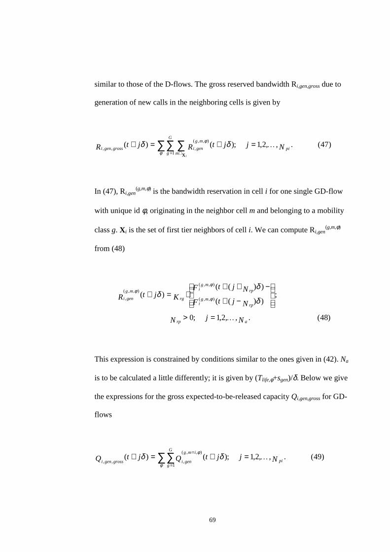
69
similar to those of the D-flows. The gross reserved bandwidth Ri,gen,gross due to
generation of new calls in the neighboring cells is given by
)47(. ,,2,1;)()(1
),,(
,,, NjjtRjtR pi
G
g m
mg
genigrossgeni
i
=+=+ ∑∑ ∑= ∈φ
φ δδX
In (47), Ri,gen(g,m,φ) is the bandwidth reservation in cell i for one single GD-flow
with unique id φ, originating in the neighbor cell m and belonging to a mobility
class g. Xi is the set of first tier neighbors of cell i. We can compute Ri,gen(g,m,φ)
from (48)
)48( . ,,2,1;0
; ))((
))(()(
),,(
),,(
),,(
,
NjN
NjtF
NjtFKjtR
arp
rpmg
i
rpmg
i
rg
mg
geni
=>
−+
−++⋅=+
δ
δδ
φ
φφ
This expression is constrained by conditions similar to the ones given in (42). Na
is to be calculated a little differently; it is given by (Tlife,φ+sgen)/δ. Below we give
the expressions for the gross expected-to-be-released capacity Qi,gen,gross for GD-
flows
)49(. ,,2,1;)()(1
),,(
,,, NjjtQjtQ pi
G
g
img
genigrossgeni=+=+ ∑∑
=
=
φ
φδδ

70
Expression (50) gives the value of expected-to-be-released capacity Qi=0,gen(g,m=i,φ)
for cell 0. Conditions similar to the ones of (45) constrain (50)
)50(. ,,2,1;0
);)((
))(()(
),,(0
),,(0
),,(
,0
NjN
NjtF
NjtFjtQ
arp
rpimg
rpimgimg
geni
=>
++
−−+=+=
==
=
δ
δδφ
φφ
Finally, the total resource reservation Ri,total in cell i at a time instant t is given by
the sum of reservations required by all D and GD type flows in all the first tier
neighboring cells
)51(. )()()(,,,
tRtRtR geniDitotali+=
Similarly, the total expected-to-be-released bandwidth Qi,total in cell i by time t is
given by
)52(. )()()(,,,
tQtQtQ geniDitotali+=
From (51) and (52) and the available capacity Ci,avail in cell i, we can calculate the
free capacity Ci,free at time t by using (53)
)53(. )()()(,,,, tQtRCtCtotalitotaliavailifreei +−=

71
The expression above can be used to predict free bandwidth in cells at any time.
We have arrived at this expression by utili zing the knowledge of cell occupancy -
user mobili ty -and call characteristics. The resource reservation scheme proceeds
as follows for the general case of cell 0.
1. As a flow is enrolled with it, cell 0 calculates the flow’s li fetime and the
values of associated branching and residual flows.
2. GD-flows are created through admission control and enrolled in cell 0. Flow
li fetime and branching/residual flow values are also computed.
3. All predictions are made for some fixed period of time – the prediction
interval.
4. Resource reservation values for N neighboring cells are calculated every δ
seconds.
5. These values of the resource reservation in the ith neighboring cell due to
flows in cell 0 are communicated to cell i via the core network.

72
6. Simultaneously with the calculation of resource reservation values, cell 0
calculates the expected-to-be-released capacity from (52) for the duration of
the projection interval.
7. Cell 0 also receives resource reservation values from its neighboring cells.
8. Cell 0 can now compute the expected free bandwidth for the duration of the
projection interval using (53).
Notice that since we do not make predictions for more than the first tier of cells,
inter-cell communication overhead in the core network is greatly reduced. Also,
we calculate branching flow values initially when a spatial flow enters a cell
through handoff or new calls. Only simple addition and subtraction steps need to
be performed after that.

73
4.3 ADMISSION CONTROL ALGORITHM
The purpose of admission control is the admission of only as many new users in
the system that can maintain the quality of service promised to users already
admitted. The admission procedure given here tests for the admissibility of a
spatial flow in its originating cell and the survivability of the composing users in
the cells they are expected to handoff to in the future. Once the flow passes the
test, composing users are allowed to complete their call. New users are
continually incorporated in the new flow and admission test is performed to verify
the feasibility of accepting the newly composed flow. This defines the
aggregation phase of the growing GD-flow. New users are incorporated up to a
period of sgen seconds after which the accumulation phase is stopped. When a
flow F0(g)(t) of class g requests admission in cell 0 at a time instant t, the
following admission test is performed before the GD-flow can be admitted.
1. Check if there is enough bandwidth in the current cell
)54(.)()( )(0,0
tFtCg
free≥
If the test of (54) holds, we proceed to the next step, otherwise we go to the
reduction step of item 4 below. C0,free is the free capacity in cell 0 at time t.
2. Check the admissibility of the flow in the current cell

74
)55(.,,2,1);()( )(0,0 NjjtFjtCK pig
a free=+≥+⋅ δδ
In this expression, Npi is the number of cycles of the resource reservation scheme
for the projection interval Tpi. Npi can be calculated from Tpi / δ. C0,free(t+jδ) is
the free capacity at time t+jδ and Ka is the admissibility constant. Ka determines
the relative weightage of admissibili ty in the originating cell for the admission
control test. With this admission test, we confirm that the flow’s admission would
not effect the QoS promised to other users admitted in the cell sometime back.
We proceed to the next step if the test is positive, otherwise the reduction step of
item 4 is executed.
3. Check the survivabilit y of the GD-flow in all the first tier neighboring cells i
)56(.,,2,1;,,2,1);()( )(,
NiNjjtFjtCK pig
ifreeis ==+≥+⋅ δδ
In essence, we calculate the branching flows of the newly formed root GD-flow
and test to see if there would be enough resources in a neighboring cell i to
support the users composing this GD-flow, if the users handoff into cell i by some
time in the future. Here, Ci,free(t+jδ) is the free capacity in cell i at time t+jδ and Ks
is the survivability constant. Ks determines the relative importance of survivabili ty
in neighboring cells for the admission control test.
75
A flow might fail the admission test due to transient overload in the home and
neighboring cells. It might be possible that the flow becomes admissible with a
lower flow bandwidth requirement. Also, to improve call blocking performance, it
may be useful to retry the admission test with a new lighter (less bandwidth
demanding) flow after blocking only some calls composing the initial flow. In the
reduction step, we block only one user’s call and form a new lighter flow. This
flow is then subjected to a similar admission test in the hope that the flow would
now be admitted. To ensure fairness, we block the most recent user call request,
so that head-of-the-queue call requests are prioriti zed.
There might be very few users requesting a call at one time. In order to
accumulate a suff icient number of users to form an economic GD-flow, we have
to wait a certain time to queue all call requests. However, it is not desirable to
make users wait for a long period to just complete their call connection. To
remedy this, we use an aggregation strategy where new call admission tests are
performed immediately and the mobile user granted access to network if the
admission test succeeds. The new call admission procedure also executes
synchronously, just like the resource reservation algorithm, with discrete steps ∆,
where ∆ is very small to provide as littl e latency as possible during the call
admission phase. For example, we may have a small value of ∆ equal to δ/5. We
form a GD type classed spatial flow with all the mobile users requesting call
during the interval [t,t+ ∆). This flow is passed through an admission test
procedure and then admitted if possible. In the next interval of [t+ ∆,t+2 ∆), any

76
new call requests belonging to the same class as the previously admitted flow are
incorporated in the old flow to form a new GD-flow. An admission test is
performed again for the new flow. If the admission test fails, only the users
requesting calls in the interval [t+ ∆,t+2 ∆) are blocked and the old GD-flow is
restored. This process is repeated for Nap∆, where Nap is given by sgen/∆. After that
time, all new call requests necessarily become part of a new GD-flow. Bandwidth
reservation can be made from the GD-flow while it is in the aggregation phase
and reservation cycle is executed. We present the pseudo-code for admission
procedure below.

77
Figure 10: Pseudo-code for admission control scheme.
Procedure AdmissionControlGiven: gen_Period, admission_Stepenable interruptRepeat for all classestime = 0num_New_User = 0flow_There = FALSE_start:interrupt if userAvailable
num_New_Users++
time += admission_Stepif time >= gen_Period
exit
if num_New_Users = 0time = 0
else_retry: if flow_There = TRUE
call addInOldFlow (num_New_Users)
elsecall formNewFlow (num_New_Users)
result = call runAdmissionTestif result = TRUE
call enrollFlowflow_There = TRUEnum_New_Users = 0
elsecall blockRecentUser (num_New_Users)num_New_Users--

78
Figure 10 (contd.): Pseudo-code for admission control scheme.
if num_New_Users > 0goto _retry
elseif flow_There = FALSE
time = 0
loop _start
Subroutines:1. addInOldFlow – adds a new user in an old flow2. formNewFlow – adds up all users to form a new flow3. runAdmissionTest – check flows for capacity,
admissibility and survivability4. enrollFlow – assigns a flow a unique id, stores flow
data and computation results5. blockRecentUser – blocks the user requesting
admission most recently

79
4.4 SECTION SUMMARY
In this section, we used the spatial flow framework of Section 3 to develop
schemes for resource reservation and admission control. Because of the
aggregating process involved in flow formation, we need to devise special
handoff methods. Specifically, handoffs can be classified as urgent or non-urgent.
Users requesting urgent handoffs must be handled with increased priority. Since
RF coverage for neighboring cells overlaps in practical cases, we can easily
implement our handoff scheme with transition regions.
Our resource reservation method proceeds by summing bandwidth/resource
demand from all flows in the neighboring cells. It also considers residual flows
inside the home cells, with which we can calculate expected-to-be-released
capacity. Final free capacity projections are obtained by combining reserved and
expected-to-be-released capacities. When calculating free capacity projections,
we use a tunable parameter to control the amount of resources that may be
reserved or released.
To support faster call setup times, we include a growing GD-flow formation
process, where new users are admitted as early as possible after performing an
admission test. If more users request admission later, they are incorporated in an
older GD-flow. This process of incorporating new users to an older flow is
discontinued after a certain period of time, after which new call originations start
forming a new GD-flow. We also control the weightage of admissibility in the

80
originating cell and survivabili ty in neighboring cells in admission control tests by
introducing two adjustable parameters – the admissibili ty constant and the
survivabili ty constant.
81
5. RELATED WORK WITH COMPARISONS
In this section, we present a brief discussion of the related work on resource
allocation and admission control in wireless cellular networks. For all the
variables and equations in this section, we use the notation used by authors of the
respective work. So the notation in this section is different from the rest of this
work.
Towards the end of this section, we also present a computational cost comparison
of all the admission control methods discussed in this section with our admission
control method. We also highlight the differences in performance and
performance-cost tradeoff throughout this section.
The amount of computation as well as communication required for performing
resource reservation and admission control is directly proportional to the amount
of information collected and made available. In our discussions about algorithmic
complexity, we determine the amount of information available or required for
performing admission control by different algorithms. This information is
required for each cell and optionally for each user. The total information required
gives a measure of computational and communication cost of the algorithm.
Algorithmic complexity for a particular algorithm will then be the total
information required by it. We present algorithmic complexity as a relative order.

82
We start with the algorithm evaluation framework of [11]. Jain and Knightly [11]
provide a resource reservation algorithm called Perfect Knowledge Algorithm
(PKA). PKA yields the best possible performance but it is physically unrealizable
since in order for the algorithm to function, we need exact information about the
future patterns of the mobility of all users. Future information cannot be made
available a-priori in real-life systems, therefore, PKA has no implementation
value. However, because PKA is optimum (it yields minimum call blocking for a
given call dropping probability), we can use it as a benchmark to compare the
performance of physically realizable systems.
PKA takes user mobility into account when calculating required bandwidth in
neighboring cells. Other algorithms (including ours) that model user mobility can
only calculate estimates of future bandwidth requirement. PKA operates under the
following three assumptions when performing admission control for a call
arriving at time t.
1. Characteristics of other calls arriving at times u>t are not known.
2. If a user is tested admissible at time t, the user must be admitted and the
decision about admission cannot be reversed at a later time.
3. Future handoffs of all admitted users are known.

83
The first two assumptions are enforced to follow the behavior of practical
admission control algorithms. We only have future information about already
admitted calls, but we cannot determine which users should request new calls
ahead of time. The goal of PKA is to maximize network utilization U, while
satisfying an empirical QoS constraint Pdrop. Defining U as the fraction of
capacity used over time, averaged over all cells, we have
)57(.)(
),(
1
1 1
∑∑ ∑
=
= ==N
j
N
j t u
jCT
tjCTU
In (57) Cu(j,t) denotes the capacity utilized in cell j at time t and C(j) is the
available capacity in cell j. N is the number of cells in the system. The empirical
handoff dropping probability Pdrop is calculated by dividing the number of
handoff failures over time by the total number of handoff attempts
(successes+failures). Note that PKA models user mobility in the sense that it
accounts for user handoff times and estimates resources for each user
individually. This is equivalent to modeling also the cell-to-cell correlation in
bandwidth occupancy. It has been shown [11] that PKA, indeed, maximizes
average utilization U. As also indicated in Section 1, however, the value of the
work of [11] mostly comes out from the recognition of the granularity differences
among different algorithms.

84
Naghshineh and Acampora [18] give a scheme for handoff support in wireless
ATM cellular networks. They consider a cellular network that can admit a
maximum of N users. If there are B cells in the network, then the probability Pi
that a particular cell has i connections established is given by (58)
)58(.)1
1()1
(BBi
NP
iNi
i −
=
−
If the cell can admit m connections without violating the QoS criteria for existing
calls, then we can calculate the cell overload probability PO from (59)
)59(.)1
1()
11(
1 1∑ ∑
+= += −
−==
N
mi
N
mi
iN
iO Bi
N
BPP
Here each user is assumed to demand the same bandwidth (as in voice calls). The
algorithm of [18] is an example of a cell-occupancy approach. User mobility is
not modeled explicitly. Instead, we are concerned with the aggregate occupancy
of the cells. Also, since the algorithm of [18] ignores user mobility, cell-to-cell
correlation in occupancy cannot be accounted for. If each user occupies 1
bandwidth unit and the total cell capacity is C, it can be shown that the
algorithmic complexity is of the order C. The amount of information needed to
calculate reservation estimates is of the same order. As we will see later, schemes
that model user mobility have a much higher algorithmic complexity,
85
consequently more information is needed and more accurate admission decisions
can be expected.
Levine et al. [19] presented a Shadow Cluster Algorithm SCA for resource
estimation and admission control in cellular wireless networks. They argue that an
active user exerts influence on the surrounding cells along the direction of travel.
We can think of the user “casting its shadow” on the nearby cells. This shadow is
where resources need to be reserved for future handoffs. The shape of the shadow
(shadow cluster of cells) is determined by user mobili ty characteristics. SCA,
thus, provides for modeling the mobili ty of individual users. However, SCA
involves calculation of required resource estimates for each user, computation of
the total reservation in each cell and communication of data between cells in
shadow clusters. For a two-dimensional cell model, such as that of Figure 5, we
can write the active probability of the user in its home cell as
)60(.)()](1[)()](1[)(2
1|:,|:,0|:,)(,,, ∑
=Υ−+Υ−=
wwjxwjxjxxMxjjx
ttGttHtP
Here Hx,M(x)(t) represents the cumulative probabilit y of the call holding time at t;
Υx,j|:0(t) is the probabili ty that the user x will stay in cell j given the call was
initiated in cell j; Υx,j|:w(t), w=1, 2 is the probabili ty that x would have left cell j
from side w by time t, given that the call was initiated in cell j; Gx,j|:w(t) is the
cumulative probabili ty of the initial cell residence time of user x in cell j, given
the call i s initiated in cell j and the user exits through side w. Active probabiliti es
86
are calculated for the cell where a user initiates the call. Active probabilities can
also be created for cells to which the user is handed off. SCA can calculate the
expected bandwidth requirement in the neighboring cells using the active
probabilities of all users in a cell. Thus, SCA resource estimation is done on per
user basis. SCA also considers user mobility and therefore, cell to cell correlation
of bandwidth occupancy. However, the fine-grained control thus achieved is
costly in terms of the amount of information processing required. Algorithmic
complexity for SCA is on the order of MN2T, where M represents the number of
users in an N cell-network. T is the average call holding time in the N-cell
network, expressed in time slots.
Whereas the algorithm of [18] is coarse-grained in that it does not provide for
modeling of cell-to-cell interactions of users, the algorithm of [19] is fine-grained
because it explicitly handles per-user mobility. The accurate admission decisions
from the fine-grained approach are obtained at the cost of increased
computational effort per user (C<MN2T). Our on-line algorithm makes an
approximation when determining user mobility characteristics. It assigns the class
characteristics to individual users but this assignment is later useful in aggregating
users into classed spatial flows. Since we do model cell to cell correlation in
occupancy resulting from user mobility, we essentially impart a finer granularity
to resource estimation and user admission decisions. On the other hand, due to
approximations in the classification stage, we expect our algorithm to show loser
admission bounds compared to schemes that are per-user mobility based, such as
87
the one in [19]. We incur much lesser algorithmic complexity and communication
overhead though. If, on average, we can aggregate A users and the computations
are performed for only the first tier of neighboring cells Nf, the algorithmic
complexity of our on-line algorithm is given by MNf2T/A. Since A>1 and Nf<N,
MNf2T/A < MN2T. The improvement in computational complexity increases with
the degree of aggregation, A. Also, our admission scheme decreases the
communication overhead since fewer values need to be passed among cells
(aggregate spatial flows vs. individual users) and fewer cells exchange
information (only the first tier neighbors). Compared to the SCA algorithm of
[19], our algorithm incurs one additional classification overhead. But the
classification overhead occurs once per several hundred iterations of the resource
allocation algorithm and therefore, the overhead diminishes to a very small
magnitude when amortized over the cycles of the admission control scheme.
As an illustration of algorithmic complexity, consider a cellular network as in
Figure 5 with C=40, N=64, M=5000, A=5, Nf=4, T=20. The following measures of
complexity for the three schemes of [18], this work and [19] respectively can be
derived: 40<320,000<409,600,000 orders. We evaluate this granularity tradeoff in
more detail in the next section.
Turning back to the classification overhead, we note that there will be variations
and periodicities in user mobility characteristics. Lets assume that we need to run
class discovery and specification procedures once every 15 minutes to account for

88
those variations. A time slot is 10 seconds long. Let us also assume that we have
1,000 user’s mobili ty parameter vectors available for that purpose. Computational
complexity for the above two processes would be 1000 x 20 / (15 x 60/10) ≈ 222
orders per cell . We also assume 5 handoffs and 5 new call originations per cell per
time slot. If user classification adds 2 orders of complexity, we have an additional
increase in complexity of 20 orders per cell . This takes us to a total increase of
222 + 20 = 242 orders in the complexity per cell . With Nf=4, we end up with 242
x 4 ≈ 1000 orders increase in algorithmic complexity (less than 1%), which is
negligible compared to the algorithmic complexity of our algorithm without
classification overhead (320,000 vs. 321,000 orders).
The following table summerizes the three schemes.
Algorithm GranularityAlgorithmicComplexity(orders of)
Sample Cost(orders of)
Communi-cation
OverheadQoS Rank*
Acampora[18] Coarse C 40 None 10
SCA[19] Fine MN2T 409600000 High 1
Our work(SFA)
Fine MNf2T/A 320000 Low 2
Table 1: Comparison of related admission control algorithms.
* QoS Rank 1 implies best QoS performance. QoS Rank 10 implies the worst
QoS performance

89
6. SIMULATION EXPERIMENTS
We have performed an extensive set of simulation experiments to test the
behavior of the spatial flow model and the SCA model of [19] under various
mobility and traffic conditions. At the end of each experiment we obtain an
empirical estimate of call dropping probability Pdrop and call blocking probability
Pblock. The call dropping probability is estimated by dividing the number of failed
handoff attempts by the total number of handoffs attempted (successful + failed
handoff attempts). The call blocking probability is calculated from the ratio of
failed call attempts and the total number of call attempts (successful + failed
attempts). Pdrop and Pblock are given on a system level and not on the cell level. We
average the values of Pdrop and Pblock for all cells in the system. Since call arrivals
as well as the distribution of traffic (users) is uniform over all cells in the system,
we do not anticipate much local congestion that could effect Pdrop and Pblock
differently in different cells. Thus, the average over all cells should give a fair
estimate of Pdrop and Pblock in any cell. Average resource utilization is an
important criterion for evaluating the performance of admission algorithms. It is
desirable for the cells to operate near 100% utilization. The average utilization
will depend on mobility characteristics of the users. Of particular importance is
the average utilization under peak traffic conditions. For example, if a cell can
carry 10 Erlangs of traffic, it is not meaningful to look at the average utilization
when the offered traffic is only 2 Erlangs. We evaluate algorithm performance
when the offered traffic is close to 10 Erlangs, say 8 or 9 Erlangs. Since the
blocking probability corresponds roughly to offered traffic, we consider average
90
utilization in a high blocking environment. Note that under certain conditions, the
admission algorithm may cause excessive resources reservation in neighboring
cells, despite there being normal traffic in the cells. Average utilization can be an
indicator of algorithm failure, but it would not indicate the ability of cells to carry
traffic with the algorithm operating normally. We also report the average
utilization for all cells. However, because of the difficulty in interpreting the
goodness of the average utilization for a given experiment, we also give the peak
average cell utilization. Peak average utilization is the maximum average
utilization over all cells. For every cell, an instantaneous utilization value is
calculated at the end of each resource reservation cycle. A running average of the
current and past values of the instantaneous utilization then yields the average
utilization for a cell. In order for one value to not effect the average greatly, we
take the average utilization by averaging the current instantaneous utilization with
several (at least last 20) past instantaneous utilization values. Finally, the mean of
average utilization over all cells is what we plot in the graphs in this section.
With resource reservation, we imply bandwidth reservation over the radio links.
Since bandwidth over radio links is the most precious resource, we assume that
other resources (like bandwidth in the core network, processor time etc.) are
readily available once radio links are turned up. The unit of bandwidth is BU
(bandwidth unit) for the purposes of our simulation experiments.

91
We have used the one dimensional service area model in our simulations. This
corresponds to a unit street or highway. We consider 10 cells in our model,
labeled 0 to 9 from left to right. Cell 0 wraps around and has a left border with
cell 9. Cell 9 wraps around to have a right border with cell 0. Users can move in
one direction after they start a call , either left or right. This restriction is a
consequence of our assumption that the users move with a “purpose” and that
there is a definite destination they pursue. However, their motion can have an up-
down component but no turn-backs, modeled by a variable horizontal speed
component. A user traveling rightward in cell 9 would ultimately be handed off to
cell 0. When new calls are originated, the user is located at a random point in the
service area in a random cell .

92
6.1 EXPERIMENTS WITH SCA
We start with experiments conducted for the algorithm of [19]. Below we give
some additional assumptions and initial conditions that we used in the
simulations.
• Only two types of users are considered (corresponding to cars and
pedestrians). This assumption does not allow for an evaluation of the mobility
classes of this work, though. But even for one type of user the mobility
parameters can vary widely. We employed two types of users to introduce
some reality into the unit street model.
• Zonoozi et. al. [13] have shown that cell residence time follows a generalized
gamma distribution. In our calculations of the active probabilities of users for
the algorithm of [19], we assumed their cells residence time to follow a
gamma distribution. However, as stated above, the mobility parameters
representing those distributions vary. When initializing the mobility
parameters, we picked values of mean cell residence times which were
uniformly distributed in a narrow range around 25 minutes for the users of
type 1 and 4 minutes for the user of type 2.
• We have assumed geographical independence of mobility parameters for all
users. In other words, a user has the same mobility characteristics for all cells
93
in the system. This assumption may not hold in real situations, but should not
cause any problems for algorithm comparison studies.
• To introduce heterogeneity in bandwidth demand, we assume that mobile
users can request four different bandwidth profiles - voice, buffered streams,
video and interactive data. But we do not model the bursty nature of some
traffic types. For example, in live video transmissions the instantaneous
bandwidth demand varies with the amount of information in a scene and with
how much of that information changes from frame to frame. In the simulation
experiments we have performed, we assume that users demand a fixed
bandwidth that remains constant throughout the duration of the call, much like
circuit switched connections. The bandwidth demand may vary from one
bandwidth profile to another. This simplifying assumption does not effect the
comparison of our admission control algorithms. It does, however, limit the
accuracy with which we can evaluate Pdrop and Pblock.
• The proportion of bandwidth profiles in the total calls a user makes may be
different. This proportion may be biased in favor of one bandwidth profile.
For example, voice calls may be the dominant part of the total calls a mobile
makes (about 80%) followed by interactive data (20%). Another user may
have all calls either being of the buffered streams or video bandwidth profile.
94
• Call holding times are considered to be distributed exponentially. Different
bandwidth profiles may have different mean call holding times. Typically,
interactive data may have a much lower mean call holding time than video.
• Call arrivals are assumed to follow a Poisson distribution. The call bandwidth
profile (video, voice etc.) is fixed at the instant of arrival. Arrival rate is the
same for all bandwidth profiles in the entire system. But that same arrival rate
for a user may be varied for all bandwidth profiles to change the offered
traffic.
• All new call requests are user terminated calls, i.e., calls originate from
outside with calling parties outside the system wanting to communicate with
mobiles inside the system.
• A user can handle one call at one time. If the user is busy and a new call
arrives for that user, that call request is simply cleared and not queued.
• For the SCA algorithm of [19], we need to specify a cluster size for the
shadow cluster of cells for which active probabilities need to be calculated.
The cluster size may vary according to the mobility characteristics of the user.
We fix the cluster size to six cells in the travel direction of the user.
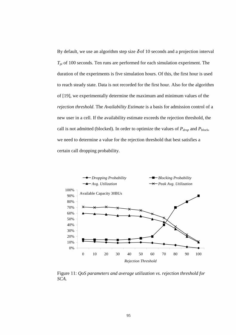
95
By default, we use an algorithm step size δ of 10 seconds and a projection interval
Tpi of 100 seconds. Ten runs are performed for each simulation experiment. The
duration of the experiments is five simulation hours. Of this, the first hour is used
to reach steady state. Data is not recorded for the first hour. Also for the algorithm
of [19], we experimentally determine the maximum and minimum values of the
rejection threshold. The Availability Estimate is a basis for admission control of a
new user in a cell. If the availability estimate exceeds the rejection threshold, the
call is not admitted (blocked). In order to optimize the values of Pdrop and Pblock,
we need to determine a value for the rejection threshold that best satisfies a
certain call dropping probability.
Figure 11: QoS parameters and average utilization vs. rejection threshold forSCA.
Available Capacity 30BUs
0%
10%
20%
30%
40%
50%
60%
70%
80%
90%
100%
0 10 20 30 40 50 60 70 80 90 100
Rejection Threshold
Dropping Probability Blocking Probability
Avg. Utilization Peak Avg. Utilization
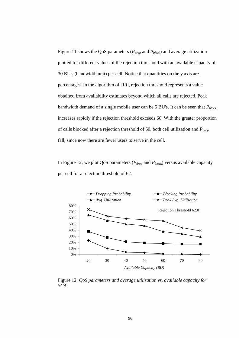
96
Figure 11 shows the QoS parameters (Pdrop and Pblock) and average utili zation
plotted for different values of the rejection threshold with an available capacity of
30 BU's (bandwidth unit) per cell . Notice that quantities on the y axis are
percentages. In the algorithm of [19], rejection threshold represents a value
obtained from availabilit y estimates beyond which all calls are rejected. Peak
bandwidth demand of a single mobile user can be 5 BU's. It can be seen that Pblock
increases rapidly if the rejection threshold exceeds 60. With the greater proportion
of calls blocked after a rejection threshold of 60, both cell utili zation and Pdrop
fall , since now there are fewer users to serve in the cell .
In Figure 12, we plot QoS parameters (Pdrop and Pblock) versus available capacity
per cell for a rejection threshold of 62.
Figure 12: QoS parameters and average utilization vs. available capacity forSCA.
Rejection Threshold 62.0
0%
10%
20%
30%
40%
50%
60%
70%
80%
20 30 40 50 60 70 80
Available Capacity (BU)
Dropping Probability Blocking Probability
Avg. Utilization Peak Avg. Utilization

97
As expected, Pdrop, Pblock, and cell util ization fall steadily with increasing value of
available capacity. The dropping probabili ty goes below one percent after the
available capacity value of 60 BU's. The call blocking probabili ty does not decay
to zero but maintains its minimum attainable value for a rejection threshold of 62
and algorithm step size δ of 10 seconds.

98
We have also experimented with different rates of call arrivals. This we achieve
by varying the intensity of offered traff ic load. We assume the arrival process to
be Poisson. Thus, a smaller value on the x axis of the chart of Figure 13 indicates
a smaller mean inter-arrival time and a greater value of offered load. The call
dropping probabili ty, the call blocking probabili ty and the cell utili zation all
increase exponentially with an increase in the call arrival rate (obtained by
reducing the mean call i nter-arrival time). The blocking probabili ty stays above
20% for a rejection threshold of 62 and an available capacity of 50 BU's.
Figure 13: QoS parameters / average utilization vs. mean call inter-arrival timefor SCA.
We next plot the QoS parameters (Pdrop and Pblock) for different values of the
projection interval of the SCA algorithm. Projection interval is the time period for
which future bandwidth reservations are estimated. It can be calculated from Npiδ.
Rejection Threshold 62.0Available Capacity 50 BU
0%10%20%30%40%50%60%70%80%
1 2 3 4 5 6 7 8 9 10 11 12 13 14 15 16
Mean Call Inter-arrival Time (min.)
Dropping Probability Blocking Probability
Avg. Utilization Peak Avg. Utilization

99
In Figure 14, Pdrop and Pblock improve sharply as the projection interval is
increased from 30 seconds to 90 seconds. The performance of the SCA seems to
become optimal around a projection interval of 90 seconds, which is equal to 9δ's.
From this point onwards, the blocking probabili ty increases with increasing
values of the projection interval. After 150-160 seconds, Pblock stabil izes at 0.7.
Pdrop also increases when the projection interval exceeds 90 seconds. Almost 70%
of all calls are not accepted into the system now. Pdrop then decreases due to fewer
numbers of active users in the system. The projection interval dependence of QoS
parameters depends on the cell residence time of the users. However, it is not easy
to quantify this relationship. We leave the determination of the optimum value of
the projection interval to experimental methods (either simulations or field data).
Notice also that longer projection intervals would mean an expenditure of greater
resources on computation, storage and communication of information.
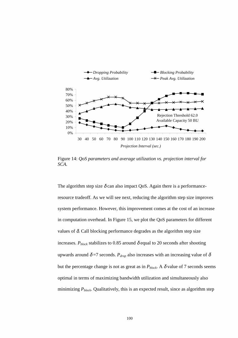
100
Figure 14: QoS parameters and average utilization vs. projection interval forSCA.
The algorithm step size δ can also impact QoS. Again there is a performance-
resource tradeoff. As we will see next, reducing the algorithm step size improves
system performance. However, this improvement comes at the cost of an increase
in computation overhead. In Figure 15, we plot the QoS parameters for different
values of δ. Call blocking performance degrades as the algorithm step size
increases. Pblock stabilizes to 0.85 around δ equal to 20 seconds after shooting
upwards around δ =7 seconds. Pdrop also increases with an increasing value of δ
but the percentage change is not as great as in Pblock. A δ value of 7 seconds seems
optimal in terms of maximizing bandwidth utilization and simultaneously also
minimizing Pblock. Qualitatively, this is an expected result, since as algorithm step
Rejection Threshold 62.0Available Capacity 50 BU
0%10%20%30%40%50%60%70%80%
30 40 50 60 70 80 90 100 110 120 130 140 150 160 170 180 190 200
Projection Interval (sec.)
Dropping Probability Blocking Probability
Avg. Utilization Peak Avg. Utilization
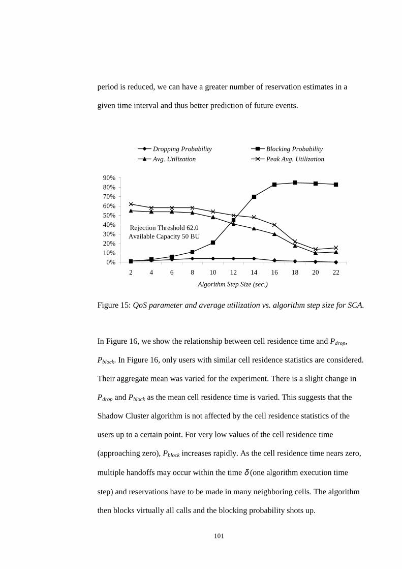
101
period is reduced, we can have a greater number of reservation estimates in a
given time interval and thus better prediction of future events.
Figure 15: QoS parameter and average utilization vs. algorithm step size for SCA.
In Figure 16, we show the relationship between cell residence time and Pdrop,
Pblock. In Figure 16, only users with similar cell residence statistics are considered.
Their aggregate mean was varied for the experiment. There is a slight change in
Pdrop and Pblock as the mean cell residence time is varied. This suggests that the
Shadow Cluster algorithm is not affected by the cell residence statistics of the
users up to a certain point. For very low values of the cell residence time
(approaching zero), Pblock increases rapidly. As the cell residence time nears zero,
multiple handoffs may occur within the time δ (one algorithm execution time
step) and reservations have to be made in many neighboring cells. The algorithm
then blocks virtually all calls and the blocking probability shots up.
Rejection Threshold 62.0Available Capacity 50 BU
0%
10%20%
30%40%
50%60%
70%80%
90%
2 4 6 8 10 12 14 16 18 20 22
Algorithm Step Size (sec.)
Dropping Probability Blocking Probability
Avg. Utilization Peak Avg. Utilization

102
Figure 16: QoS parameters / utilization vs. mean aggregate cell residence time forSCA.
Rejection Threshold 62.0Available Capacity 50 BU
0%10%20%30%40%50%60%70%80%90%
100%
1 3 5 7 9 11 13 15 17 19 21
Mean Aggregate Cell Residence Time (min.)
Dropping Probability Blocking Probability
Avg. Utilization Peak Avg. Utilization
103
6.2 EXPERIMENTS WITH SPATIAL FLOWS ALGORITHM
In this sub-section, we present the results of simulation experiments with our
classed spatial flows algorithm (SFA). We have endevoured to maintain
conditions similar to those that were used when we experimented with the SCA of
[19]. However, are a few differences, which are explained below.
We have used three mobili ty classes in all experiments with our algorithm but we
did not perform class determination. Instead, we fixed the class specification (i.e.,
the class mobili ty parameter vector) for a mobili ty class, then generated the
mobili ty parameter vector for every user in that class. We assumed the parameter
variation to be Gaussian. This is in line with the multi -variate normal assumption
of linear or quadratic discriminants of our user classification scheme. Thus, both
cell residence time and handoff probabiliti es for each user was a random variable,
distributed normally about the class means. Thus, the mobili ty classes were a
mean representation of composing users. We employed user mobili ty parameter
vectors to simulate user’s motion in the service area. For admission control and
resource reservation, we used class mobili ty parameter vectors only.
The simulation experiments we performed for the spatial flows algorithm aims to
evaluate the performance of our admission control and resource reservation
schemes.
Unlike the SCA, we make resource reservation in the first tier neighboring cells
only. For the one-dimensional service area for which we performed our

104
experiments, we made reservations in the immediate left and right neighboring
cells.
Our approach is to change one variable in one experiment at a time and fix all
other variables for the same experiment. Unless it is being varied in an
experiment, the default variable values are: normalized reservation period = 2,
reservation gain = 5, admissibility constant = 1, survivability constant = 1,
available capacity = 30 BU, mean call inter-arrival time = 3 minutes, handoff
urgency factor = 2, algorithm step size = 10 seconds and projection interval = 100
seconds.
Figure 17: QoS parameters and utilization vs. normalized reservation period forSFA.
Available Capacity 30 BU
0
10
20
30
40
50
60
70
80
1 2 3 4 5 6 7 8 9
Normalized Reservation Period
Uti
liza
tion
(%
)
1
2
3
4
5
6
7
8P
roba
bili
ty (
%)
Avg. Utilization Peak Avg. Utilization
Blocking Probability Dropping Probability
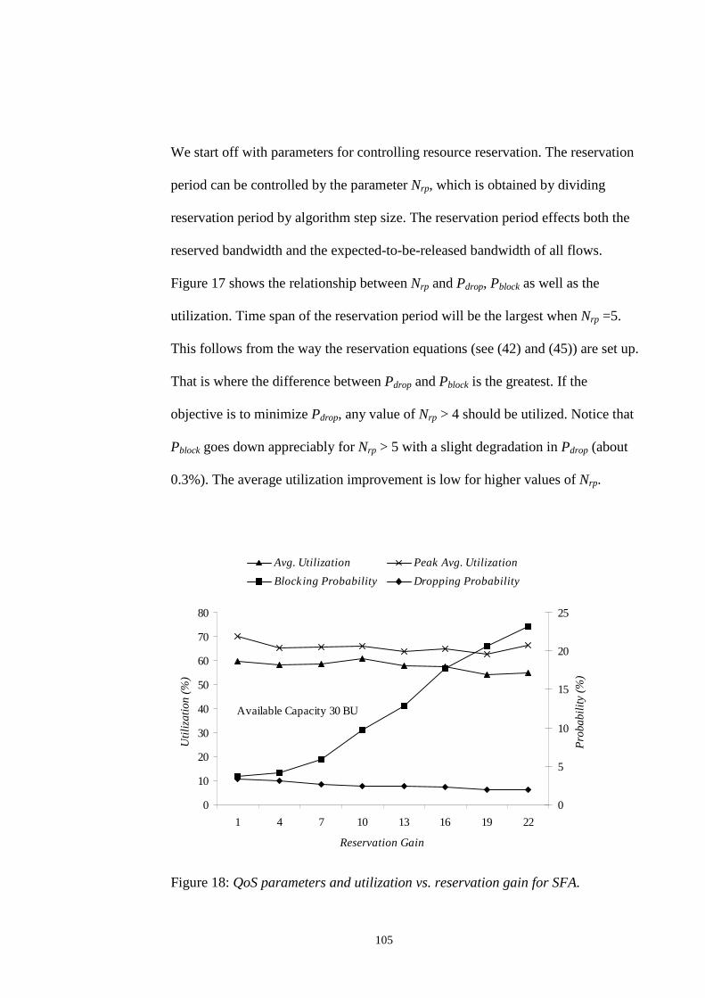
105
We start off with parameters for controlling resource reservation. The reservation
period can be controlled by the parameter Nrp, which is obtained by dividing
reservation period by algorithm step size. The reservation period effects both the
reserved bandwidth and the expected-to-be-released bandwidth of all flows.
Figure 17 shows the relationship between Nrp and Pdrop, Pblock as well as the
utilization. Time span of the reservation period will be the largest when Nrp =5.
This follows from the way the reservation equations (see (42) and (45)) are set up.
That is where the difference between Pdrop and Pblock is the greatest. If the
objective is to minimize Pdrop, any value of Nrp > 4 should be utilized. Notice that
Pblock goes down appreciably for Nrp > 5 with a slight degradation in Pdrop (about
0.3%). The average utilization improvement is low for higher values of Nrp.
Figure 18: QoS parameters and utilization vs. reservation gain for SFA.
Available Capacity 30 BU
0
10
20
30
40
50
60
70
80
1 4 7 10 13 16 19 22
Reservation Gain
Uti
liza
tion
(%
)
0
5
10
15
20
25
Pro
babi
lity
(%
)
Avg. Utilization Peak Avg. Utilization
Blocking Probability Dropping Probability

106
In the graph of Figure 18, we have plotted the blocking and dropping probabilities
as well as system resource utilization for different values of the reservation gain.
Recall that the Reservation gain effects only the reserved capacity. Notice that
only a slight improvement in Pdrop is achieved for a large degradation in system
blocking performance. The Pdrop improvement in going from no gain (reservation
gain = 1) to a 22 fold gain is 42%, but this is obtained at a cost of a 531%
degradation in Pblock. We fixed the reservation gain value to 5 for all other
experiments, since that seems to be an optimal tradeoff point. However, the
reservation gain allows an opportunity to trade off the blocking performance for
better dropping performance and may be used if required.
Figure 19: QoS parameters and utilization vs. admissibility constant for SFA.
Available Capacity 30 BU
0
10
20
30
40
50
60
70
80
0 0.1 0.3 0.5 0.7 0.9 1.1 1.3 1.5 1.7 1.9
Admissibility Constant
Uti
liza
tion
(%
)
1
2
3
4
5
6
7
8
Pro
babi
lity
(%
)
Avg. Utilization Peak Avg. Utilization
Blocking Probability Dropping Probability

107
Next we turn to the two parameters that impact admission control. In Figure 19,
we plot Pdrop, Pblock and resource utilization for different values of the
admissibility constant. The admissibility constant fixes the relative weightage of
admissibility in the home cell. Before admitting a new GD-flow, we test to see if
the residual flow from the new GD-flow will take more resources in the cell than
what might be available after subtracting the requirements for existing flows and
users that may be handing off into the cell. The admissibility constant emphasizes
or de-emphasizes that test. From Figure 19, it is obvious that Pblock can be traded
off against Pdrop for higher values of the admissibility constant. An interesting
case is that of the admissibility constant = 0, which means that the admissibility
test will always be successful. This means that flows would be accepted even if
they would normally (with a non-zero admissibility constant) violate the
admissibility test. We can see that there is a marked increase in Pblock from no
admissibility test (Admissibility Constant = 0) to some level of admissibility test
(Admissibility Constant = 0.1). After an initial sharp rise, Pblock varies almost
linearly with the admissibility constant. Pdrop also decreases almost linearly with
the admissibility constant, with a negative slope about equal in magnitude to the
positive slope of the Pblock curve.

108
Figure 20: QoS parameters and utilization vs. survivability constant for SFA.
Figure 20 shows the relationship between the second admission control impacting
parameter, the survivability constant and Pdrop, Pblock as well as the resource
utilization. Most noteworthy is the case of a survivability constant value of 0.
Recall that the survivability constant fixes the relative importance of the
survivability test in admission control. The survivability test is performed to find
out if the mobiles composing the new GD-flow will be able to handoff to another
cell without dropping calls. A survivability constant value of zero implies that the
survivability test is always successful. This means that new GD-flows will be
accepted even if they would normally (normal case of a non-zero survivability
constant) fail the survivability test. From the curve of blocking probability in
Figure 20, it is clear that Pblock shows a step rise from a survivability constant
Available Capacity 30 BU
0
10
20
30
40
50
60
70
80
0 0.1 0.3 0.5 0.7 0.9 1.1 1.3 1.5 1.7 1.9
Survivability Constant
Uti
liza
tion
(%
)
1
2
3
4
5
6
7
8
Pro
babi
lity
(%
)
Avg. Utilization Peak Avg. Utilization
Blocking Probability Dropping Probability
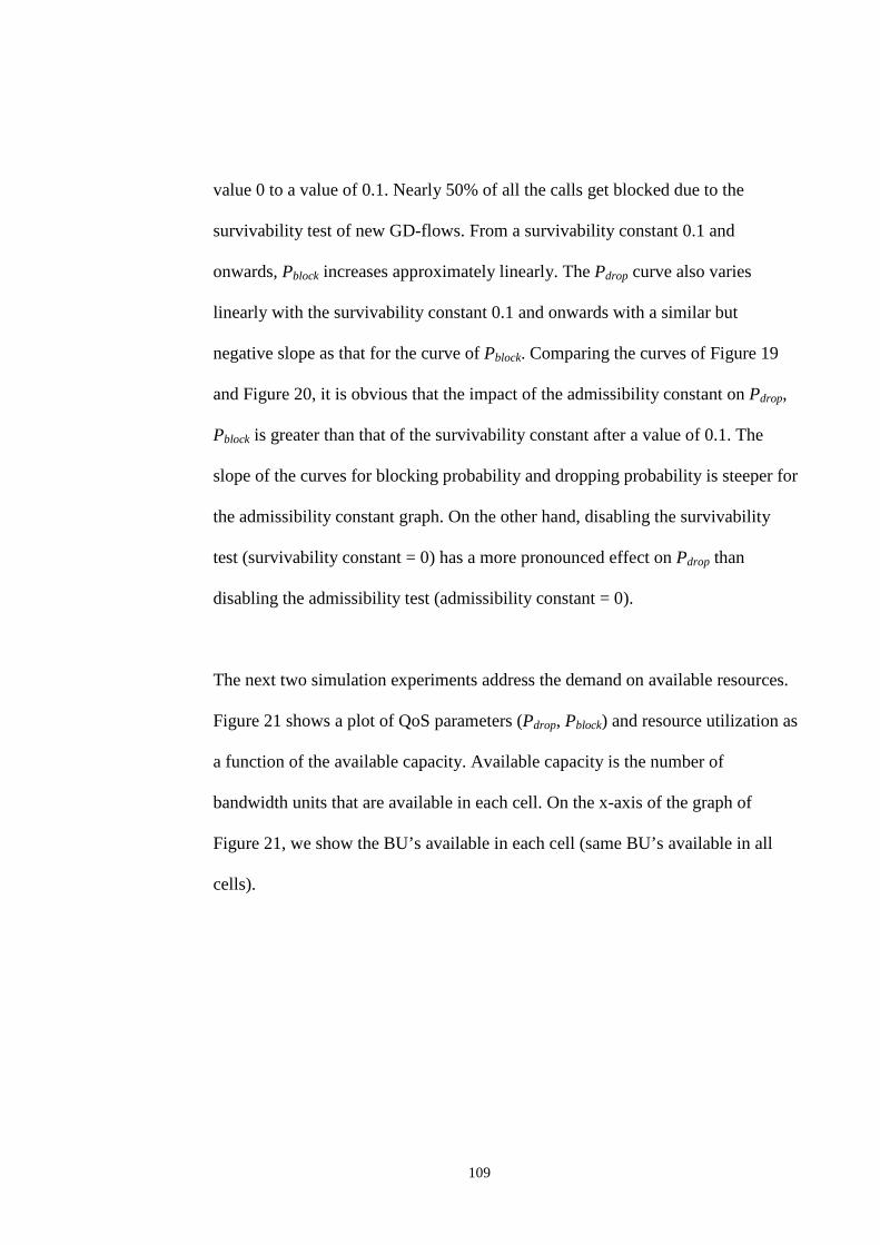
109
value 0 to a value of 0.1. Nearly 50% of all the calls get blocked due to the
survivabili ty test of new GD-flows. From a survivabili ty constant 0.1 and
onwards, Pblock increases approximately linearly. The Pdrop curve also varies
linearly with the survivabili ty constant 0.1 and onwards with a similar but
negative slope as that for the curve of Pblock. Comparing the curves of Figure 19
and Figure 20, it is obvious that the impact of the admissibili ty constant on Pdrop,
Pblock is greater than that of the survivabili ty constant after a value of 0.1. The
slope of the curves for blocking probabili ty and dropping probabili ty is steeper for
the admissibili ty constant graph. On the other hand, disabling the survivabili ty
test (survivabili ty constant = 0) has a more pronounced effect on Pdrop than
disabling the admissibilit y test (admissibili ty constant = 0).
The next two simulation experiments address the demand on available resources.
Figure 21 shows a plot of QoS parameters (Pdrop, Pblock) and resource utili zation as
a function of the available capacity. Available capacity is the number of
bandwidth units that are available in each cell . On the x-axis of the graph of
Figure 21, we show the BU’s available in each cell (same BU’s available in all
cells).
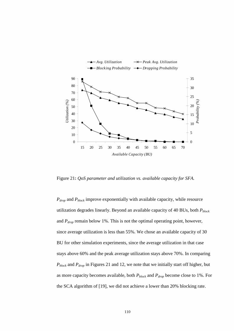
110
Figure 21: QoS parameter and utilization vs. available capacity for SFA.
Pdrop and Pblock improve exponentially with available capacity, while resource
utilization degrades linearly. Beyond an available capacity of 40 BUs, both Pblock
and Pdrop remain below 1%. This is not the optimal operating point, however,
since average utilization is less than 55%. We chose an available capacity of 30
BU for other simulation experiments, since the average utilization in that case
stays above 60% and the peak average utilization stays above 70%. In comparing
Pblock and Pdrop in Figures 21 and 12, we note that we initially start off higher, but
as more capacity becomes available, both Pblock and Pdrop become close to 1%. For
the SCA algorithm of [19], we did not achieve a lower than 20% blocking rate.
0
10
20
30
40
50
60
70
80
90
15 20 25 30 35 40 45 50 55 60 65 70
Available Capacity (BU)
Uti
liza
tion
(%
)
0
5
10
15
20
25
30
35
Pro
babi
lity
(%
)
Avg. Utilization Peak Avg. Utilization
Blocking Probability Dropping Probability
111
Figure 22: QoS parameters and utilization vs. mean call inter-arrival time forSFA.
The mean call inter-arrival time is the average call inter-arrival time over all
users. Call arrivals are assumed to follow a Poisson distribution, therefore, this
aggregate mean over all users represents the mean of an exponential distribution.
Lower values on the x-axis of Figure 22 represent higher call arrival rates. Thus,
offered traffic intensity decreases as we go farther on the x-axis of the graph in
Figure 22. The curves for Pblock as well as Pdrop are nearly exponential. Resource
utilization falls linearly as mean call inter-arrival time is increased. Note that for
low arrival rates (inter-arrival time > 8 minutes), both Pblock and Pdrop become less
than 1%. Corresponding values for resource utilization will give a measure of the
loading of the system. Note that this behavior is the same as what we obtained for
Available Capacity 30 BU
0
10
20
30
40
50
60
70
80
1 2 3 4 5 6 7 8 9 10 11 12 13 14 15
Mean Call Inter-arrival Time (min.)
Uti
liza
tion
(%
)
0
2
4
6
8
10
12
14
16
18
20
Pro
babi
lity
(%
)
Avg. Utilization Peak Avg. Utilization
Blocking Probability Dropping Probability

112
the SCA scheme of [19] (see Figure 13). There too, the dropping probability
becomes less than 1% for a mean call inter-arrival time greater than 8 minutes.
However, Pblock stabilizes around 20% there. This blocking figure may go to a
lower level for a lower value of the rejection threshold.

113
We included a handoff urgency factor in our simulation experiments. This
parameter is used to mark users for urgent handoffs. When a user is marked for
urgent handoff, it is given priority for handoff purposes. Users that are near cell
edge (cell border + transition region) will normally be marked for urgent
handoffs. Handoff urgency factor values greater than 0 will expedite marking of
urgent handoffs. This means that users will be marked for urgent handoffs much
earlier and before they reach the cell edge.
Figure 23: QoS parameter and utilization vs. handoff urgency factor for SFA.
Available Capacity 30 BU
0
10
20
30
40
50
60
70
80
0 0.25 0.5 0.75 1 1.25 1.5 1.75 2 2.25 2.5
Handoff Urgency Factor
Uti
liza
tion
(%
)
1
2
3
4
5
6
7
8
Pro
babi
lity
(%
)
Avg. Utilization Peak Avg. Utilization
Blocking Probability Dropping Probability

114
Once the user crosses the cell edge and it cannot be handed off, it will drop the
call in progress. Figure 23 shows Pdrop, Pblock and resource utilization for different
values of the handoff urgency factor. We notice only a slight improvement as the
urgency factor values are increased. There is a more noticeable performance
degradation as the handoff urgency is disabled (handoff urgency factor = 0).
Figure 24: QoS parameters and utilization vs. algorithm step size for SFA.
The algorithm step size determines how often the resource reservation and
admission control algorithm will be executed. The algorithm step size δ will
determine the cost of execution. Through algorithm step size, we can trade off
cost with accuracy of the admission control decisions. In Figure 24, we plot Pblock
and Pdrop as well as resource utilization for increasing values of the algorithm step
Available Capacity 30 BU
0
10
20
30
40
50
60
70
80
2 4 6 8 10 12 14 16 18 20
Algorithm Step Size (sec.)
Uti
liza
tion
(%
)
1
3
5
7
9
11
Pro
babi
lity
(%
)
Avg. Utilization Peak Avg. Utilization
Blocking Probability Dropping Probability

115
size. As δ is increased, both blocking and dropping performance degrades. δ =6
seconds seems to be optimal, since we reduce the cost of the algorithm
implementation without sacrificing blocking performance. We chose a value of δ
=10 seconds for all other simulation experiments. Beyond an algorithm step size
of 18 seconds, further increasing δ is prohibitively expensive on system blocking
performance, even though the dropping probability gets better. We can compare
the graph of Figure 24 with that of Figure 15 for the algorithm of [19]. Notice that
Pblock approaches 1% for δ =2 seconds. It remains lower than what we obtained
for the SFA in Figure 24 up to δ =6 seconds. For that δ >10 seconds, blocking
performance becomes unstable. Our algorithm does not show this type of
instability in blocking performance, but it performs less efficiently for δ <6
seconds. In fact even at δ =40 seconds, our algorithm operates at a high utilization
while maintaining a blocking probability of 12.2% with a low dropping
probability of 3.1%.

116
Figure 25: QoS parameters and utilization vs. projection interval of SFA.
In Figure 25, we plot Pdrop, Pblock and resource utilization against the projection
interval. We notice that there is only a very slight improvement in blocking as
well as dropping performance as the projection interval is increased beyond 30
seconds. This is contrary to what we obtained for the algorithm of [19] (see
Figure 14). For the algorithm of [19], we have a gradual performance
improvement up to a projection interval of 90 seconds, after which we saw rapid
performance degradation. Our algorithm is almost neutral to the projection
interval.
Our algorithm offers a multi-dimensional control facility. Although the cellular
wireless system with mobile users is highly complex and non-linear, results of the
Available Capacity 30 BU
0
10
20
30
40
50
60
70
80
30 40 50 60 70 80 90 100 110 120 130 140 150 160 170 180
Projection Interval (sec.)
Uti
liza
tion
(%
)
1
2
3
4
5
6
7
8
Pro
babi
lity
(%
)
Avg. Utilization Peak Avg. Utilization
Blocking Probability Dropping Probability

117
simulation on the one-dimensional model we employed show that from a system
performance viewpoint, we may model the wireless cellular system as a linear
system in certain cases. Specifically, we have the following conclusions.
• Pdrop and Pblock are optimal at a normalized reservation period Nrp of 5.
Otherwise, the variation is not linear. Nrp=5 corresponds to the middle of the
reservation period.
• Pdrop varies linearly with the reservation gain Krg. Pblock is not linear with Krg.
The variation is exponential initially and then linear.
• Both Pdrop and Pblock vary linearly with the admissibility constant Ka for Ka >0.
• Pdrop and Pblock also vary linearly with the survivability constant Ks for Ks >0.
• Pdrop and Pblock also vary more or less linearly with the algorithm step size δ.
• There is little impact of varying the projection interval.
• With available capacity, both Pdrop and Pblock vary exponentially. Resource
utilization varies in a more linear fashion.
• Both Pdrop and Pblock vary exponentially with offered traffic. Resource
utilization varies in a more linear fashion.
Out of the eight control options listed above, the last two parameters need to be
fixed initially when designing the system. The first six options can be used in
real-time system performance control, although it is not desirable to change the
algorithm step size too often. However, there may be some problems with this
approach. First, the form of linear relationships changes with time and as newer

118
network elements are added. There are long term permanent variations as well as
short term temporary and periodic variations. It is difficult to come up with
analytical expressions for controlling the QoS performance. Instead we have to
rely on simulations or field data. Each time the network is reconfigured there will
be a need to perform new simulations to estimate control relationships. We can
form a closed loop performance control system which strives to maintain a certain
level of QoS performance and resource utilization by feeding back Pdrop and Pblock
to control system performance.
The size of transition region determines the time that is available to hold calls
while a handoff is in progress. If the transition region is wider, more time will be
available to complete the handoff. Our handoff algorithm will maintain a call in
the old cell as long as the user is in the transition region between the old cell and
the cell towards which the user is traveling. Calls are dropped due to lack of
resources in the new cell only when the user crosses over into the new cell after
leaving the transition region. Thus, wider transition regions will allow the calls to
be maintained longer even with congestion in the handoff cells. Pdrop can be
improved significantly with wider transition regions without effecting Pblock much.
Wider transition regions can help offset temporary congestion in handoff cells.
Wider transition regions can also help in aggregation of D-flows during handoffs.
This means that a greater number of users may be aggregated in wider transition
regions, because more time is available before the users must be handed off into
new cells to avoid dropped calls. A greater degree of aggregation would make the
119
algorithm execution more efficient. However, there is a limit to the size of the
transition region owing to the practical considerations of RF signal propagation
and interference. Validity of the spatial flows, in terms of their goodness in
representing resource demand, may also be compromised with very wide
transition regions. This would then effect the resource reservation and call
admission decisions to degrade the QoS performance.
Number of cells in the service area of the simulation experiments should not
effect the QoS performance of the system (as long as the average number of users
in the cell remain constant) since the QoS parameters Pdrop and Pblock are
determined on per cell basis and so the number of cells do not matter. However, if
the number of users per cell is increased without changing the available capacity
in each cell, Pdrop and Pblock will both be degraded. The same effect was obtained
by varying the available capacity per cell while fixing the number of users
(Figures 21 and 12). It can be seen clearly that the QoS performance will degrade
simply because there is less bandwidth per user as available capacity in the cell is
decreased. Bandwidth per user per cell is a key metric in this regard. If we keep
the bandwidth per user per cell fixed and increase the number of users per cell
(equivalent to increasing the number of users as well as available capacity in the
cell), we should not notice any degradation in QoS performance. We can expect
to see an improvement in algorithm execution efficiency because of the greater
degree of aggregation in that case. QoS performance may also improve slightly
for the same reason.
120
We used a uniform distribution at the time of call origination to place the user in a
cell in the service area and to determine the location of the user in that cell. This
means that users will be distributed uniformly over the service area in the long
term. There will still be hot spots, where temporary congestion may result. This
contrasts to a scheme where users are placed in a deterministic round-robin
fashion. The later scheme will result in a more even distribution of users and a
lesser chance of local temporary congestion in a cell, thus, resulting in a smaller
number of dropped calls. We can deliberately create a situation where there are
persistent hot spots and congestion in certain cells. This kind of user distribution
will cause a larger number of dropped calls due to handoff requests in resource
deficient cells. Also, this distribution models the service area more accurately.
There are traffic hotspots such as office buildings and shopping areas. In case of
non-uniform traffic distribution, we can expect to see an increase in Pdrop.
Finally, we expect the results of simulation experiments to be different for a two
dimensional service area. Since for the two dimensional flows there are more
branches and consequently less certainity, we can expect a minor degradation in
the QoS performance. The degree of aggregation of D-flows may also be reduced
for the same number of users per cell because the users will have two additional
cells to where they can be handed off. In the more often employed case of two
dimensional cell grid, we may see a degradation of QoS performance further
because of greater uncertainity of handoffs. In a hexagonal grid each cell has six

121
neighbors, thus handoff probabilities may be smaller. However, field experience
suggests that handoffs happen predominantly between neighbor cells that are
connected by roadways. In practice, even for a hexagonal grid, only one or two
neighbor cells may be handing off users. Also, for practical considerations, it is
hard to enforce a hexagonal grid shape in a real service area. For all these reasons,
rectangular cell grids offer a good alternative for service area modeling. For
further discussion of service area modeling see [12].

122
7. CONCLUSION
In this thesis, we have developed a methodology for classifying users in a mobile
wireless cellular network based on their mobility characteristics. We then used
this mobility classification technique to aggregate users into classed spatial flows.
We developed a framework of spatial flows. The spatial flow framework was
employed to perform resource reservation and admission control for a wireless
cellular mobile network. Computational complexity of our algorithm is much
lower than other fine-grained approaches. This was achieved at the cost of lower
algorithm accuracy. We performed an extensive set of simulations to evaluate this
granularity-accuracy tradeoff. Simulation experiments were performed for the
algorithm developed in this thesis as well as for the other fine-grained algorithm
of [19]. Results of experiments reveal that our algorithm performs almost as well
as the other fine-grained approach, at the same time it avoids any instabilities. We
also proposed a multi-dimensional strategy to control the performance of a
cellular wireless network that utilizes our algorithm for admission control.
Our algorithm requires that the cells do the following.
• Cache the mobility vector xmob of the users visiting the cell in a particular
interval of time.
• Execute class discovery and class specification procedure periodically to
determine the mobility class structure in the cell.
• Query users originating new calls and users handed off into the cell about
their mobility vector xmob.
123
• Determine the mobility class of the users.
• Form spatial flows from users currently in the cell.
• Calculate the branching and residual flows of all the spatial flows present at
one time in the cell.
• Calculate the bandwidth required in the neighboring cell from all the
branching flows destined towards that neighboring cell and communicate the
information to the neighboring cell.
• The cell obtains, from the neighboring cell, information regarding bandwidth
from branching flows in the neighboring cell that are destined to be handed
off to the cell.
• Update the free capacity situation in the cell.
The users are required to do the following.
• Measure the members of mobility vector xmob for each cell visited and cache
that value.
• Provide the xmob vector to the current cell when queried.
In order to model the mobility of users accurately, the space-time dependent user
mobility characteristics (i.e., xmob vector) need to be stored both by the cell and
the mobile user. However this should not create any scalability issues for the user,
since xmob may be cached for more recently visited or most often visited cells. At
the cell level, only the past few thousand vectors are needed for accurate mobility
characterization of the users. Because parametric probability distributions are
124
employed, only a few bytes are required for caching one vector. For these reasons
all fine grained algorithms, including ours, are scalable.
Finally, as the results of simulations show, we can compare our algorithm with
other fine grained approaches as follows.
• Our algorithm shows similar QoS performance as other fine-grained
approaches.
• Our algorithm is more than 1000 times less computationally intensive. This
figure includes the mobility classification overhead.
• Our algorithm has a more stable Pblock performance.
• We incur less communication overhead.
• Our algorithm involves the same input data and input caching requirements.
However, storage needed in the cells at run-time should be lower, since then
we deal with flows and not individual users.
• We also offer more options for controlling QoS performance.

125
8. REFERENCES
1. Admission Control for Statistical QoS: Theory and Practice. E. Knightly, N.
Shroff. Technical Report, Rice University, 1999.
2. Deterministic Delay Bounds for VBR Video in Packet Switching Networks:
Fundamental Limits and Practical Tradeoffs. D. Wrege, E. Knightly, H.
Zhang, J. Liebeherr. IEEE/ACM Transactions on Networking, 4(3), pp. 352-
362, June 1996.
3. Fair Queueing in Wireless Packet Networks. S. Lu, V. Bhargavan. In
Proceedings of ACM SIGCOMM 97, Cannes France, September 1997
4. Packet Fair Queueing Algorithms for Wireless Networks with Location
Dependent Errors. T. Ng, I. Stoica, H. Zhang. In Proceedings of IEEE
INFOCOMM 98, San Francisco CA, March 1998.
5. Wireless Communications, Principles and Practice. T. Rappaport. Prentice
Hall PTR, 1996, pp. 35, 481.
6. Reservation Strategies for Multimedia Traffic in a Wireless Environment. B.
Epstein, M. Schwartz. IEEE Conference Proceedings 0-7803-2742-X/95,
1995.
7. Modeling the Handoff Problem in Personal Communication Networks. S.
Rappaport. IEEE Conference Proceedings CH2944-7/91/0000/0517, 1991.
126
8. Performance of Personal Portable Radio Telephone Systems with and without
Guard Channels. C. Yoon, C. Un. IEEE JSAC, Vol. 11, No. 6, August 1993,
pp. 911-917.
9. Multiple Call Handoff Problem with Queued Handoffs and Mixed Platform
Types. C. Purzynski, S. Rappaport. IEEE Proc.-Commun., Vol. 142, No. 1,
Feburary 1995.
10. Control and Quality-of-Service Provisioning in High Speed Microcellular
Networks. A. Acampora, M. Naghshineh. IEEE Personal Communications,
Second Quarter 1994.
11. A Framework for Design and Evaluation of Admission Control Algorithms in
Multi-Service Mobile Networks. R. Jain, E. Knightly. In Proceedings of IEEE
INFOCOM 99.
12. Mobility Modeling in Third Generation Mobile Telecommunication Systems.
J. Markoulidakis, G. Lyberopoulos, D. Tsirkas, E. Sykes. IEEE Personal
Communications, pp. 41-56, August 1997.
13. User Mobility Modeling and Characterization of Mobility Patterns. M.
Zonoozi, P. Dassanayake. IEEE JSAC, Vol. 15, No. 7, pp. 1239-1252,
September 1997.
14. A Model for Teletraffic Performance and Channel Holding Time
Characterization in Wireless Cellular Communications with General Session

127
and Dwell Time Distributions. P. Orlik, S. Rappoport. IEEE JSAC, Vol. 16,
No. 5, June 1998, pp. 788-803.
15. Connection Admission Control for Mobile Multiple-Class Personal
Communication Networks. C. Chao, W. Chen. IEEE JSAC, Vol. 15, No. 8,
pp. 1618-1626, 1997.
16. New Call Blocking versus Handoff Blocking in Cellular Networks. M. Sidi,
D. Starobinski. Wireless Networks, Vol. 3, pp. 15-27, 1997.
17. A Stochastic Model to Capture Space and Time Dynamics in Wireless
Communication Systems. W. Massey, W. Whitt. AT&T Bell Labs Technical
Report, April 1994.
18. An Architecture and Methodology for Mobile-Executed Handoff in Cellular
ATM Networks. A. Acampora, M. Naghshineh. IEEE JSAC, Vol. 12, pp.
1365-1374, October 1994.
19. A Resource Estimation and Call Admission Algorithm for Wireless
Multimedia Networks using the Shadow Cluster Concept. D. Levine, I.
Akyildiz, M. Naghshineh. IEEE/ACM Transactions on Networking, Vol. 5,
No. 1, pp. 1-12, February 1997.
20. Stanford University Mobile Activity TRAces,
http://wwwdb.stanford.edu/pleiades/SUMATRA.html.

128
21. Discriminant Analysis and Statistical Pattern Recognition. G. McLachlan.
John Wiley and Sons, Inc., 1992.
22. Predictive and Adaptive Bandwidth Reservation for Handoffs in QoS-
Sensitive Cellular Networks. S. Choi, K. Shin. In Proceedings of ACM
SIGCOMM 98, Vancouver British Columbia, 1998.
23. Supporting Real-Time Applications in an Integrated Service Packet Network:
Architecture and Mechanism. D. Clark, S. Shenker, L. Zhang. In Proceedings
of ACM SIGCOMM 92, pp. 14-26, Baltimore Maryland, August 1992.
24. A Scheme for Real-Time Channel Establishment in Wide-Area Networks. D.
Ferrari, D. Verma. IEEE JSAC, 8(3): 368-379, April 1990.
25. Control of Resources in Broadband Networks with Quality of Service
Guarantees. A. Lazar, G. Pacifici. IEEE Communications, pp. 66-73, October
1991.
26. Effect of Mobility on QoS in Wireless Communication Networks. M. Cheung,
J. Mark. IEEE Conference Proceedings 0-7803-4314X/98, 1998.
27. Properties of the Estimators for the Gamma Distribution. K. Bowman, L.
Shenton. Marcel Dekker, Inc., Chapter 1, pp. 8-9.
28. Queuing Systems, Vol. 1&2, L. Kleinrock, John Wiley and Sons, Inc., 1975-
76.


