
ADDIS ABABA UNIVERSITY
A NEW METHOD OF NOTCHING IN VIBRATION
CONTROL
by
Tollossa Deberie
A Thesis submitted to the School of Graduate Studies of Addis Ababa University in partial
fulfilment of the requirements for the Degree of Masters of Science in Mechanical Engineering
(Applied Mechanics stream)
Advisor
Dr. A.Raman
MECHANICAL ENGINEERING DEPARTMENT
ADDIS ABABA UNIVERSITY
OCTOBER 2007

ii

iii
Abstract
The traditional vibration test methodology of controlling the interface environment only to a
motion based specification is often too conservative, inducing potentially excessive vibration
responses at hardware resonant frequencies. This over testing problem occurs because the
smooth, input acceleration specification used in the test configuration is characteristic of a rigid,
infinite impedance equipment mount; and not characteristic of the compliant, finite impedance
equipment mount more typical of the service configuration. Recently, the so called Force Limited
Vibration (FLV) testing developed at the Jet Propulsion Laboratory offers many opportunities to
decrease the over testing problem associated with traditional vibration testing. FLV testing
methodology, controls the input acceleration and limits the reaction forces between the test item
and the shaker through real-time notching of the input acceleration, is often hard subject to apply
the force gauges. This problem has been recognized in this work and the energy limiting
vibration test methodology has recently emerged as a viable solution which makes use of stress
feedback signal to the vibration control loop using strain gauges that are trouble-free to the
functions they are meant to perform. The underlying theoretical basis of the energy limiting
vibration testing technique is the strain energy value which is the integration of product of von-
mises stress and strain over an element is a parameter prime important since it is related to the
total amount of energy transmitted to the test item during the vibration. To illustrate this
methodology, a case study of a typical satellite presented to prove the effectiveness. A procedure
was proposed to identify the topological location of notch channels or critical locations using
FEM results of the base excitation, so as to enable the vibration control mechanism to adjust the
power input of shaker table. The base excited dynamic response analysis yielded the percentage
reduction of shaker power. The notching of the force limiting and energy limiting vibration
testing methods were compared and founded incomparable even though it is acceptable.

iv
Acknowledgements
First, many thanks to my advisor, Dr. A. Raman, for getting me started on the path that this
research has taken. His inspiration and guidance through out the year has been invaluable in the
conception and design of the new idea. I am looking forward to several more years of exploration
and research under his guidance.
I would also like to thank the staffs of the department, both past and present. You have all
endowed me with the knowledge and skill in my education in engineering from the beginning to
this level and made this research successful.
In the faculty Library, I would also like to thank the staff as a whole for I got through all the
materials the library has these two years and even got electronics library.
There are my class mates who I would like to thank for their conversations, support, and general
friendship.
Finally, I would like to thank my entire friends, my family for encouraging me through these
many years of school. They have all been a tremendous source of support and encouragement
throughout all of this work. I appreciate their interest in my research.

v
Table of Contents
Approval Page..................................................................................................................... ii
Abstract .............................................................................................................................. iii Acknowledgements.............................................................................................................iv Table of Contents.................................................................................................................v
List of Tables .................................................................................................................... vii List of Figures.................................................................................................................. viii List of Symbols....................................................................................................................x
CHAPTER ONE: INTRODUCTION..................................................................................1 1.1 Background................................................................................................................1
1.2 Vibration Exciters......................................................................................................3 1.2.1 Shaker Controllers .............................................................................................4 1.2.2 Vibration Test Fixture .......................................................................................6 1.2.3 Instrumentation..................................................................................................8
1.2.3.1 Piezo-electric Force Transducers.............................................................8 1.2.3.2 Strain Gages...........................................................................................10
1.3 Thesis Objectives.....................................................................................................12 1.4 Thesis Statement......................................................................................................13 1.5 Thesis Organization .................................................................................................13
CHAPTER TWO: LITERATURE REVIEW....................................................................14
CHAPTER THREE: THEORETICAL BASIS .................................................................22
3.1 The Vibration Over Testing Problem ......................................................................22 3.1.1 Impedance Simulation.....................................................................................22 3.1.2 Response Limiting...........................................................................................23
3.1.3 Force Limiting.................................................................................................25 3.1.4 Enveloping Tradition.......................................................................................25
3.1.5 Dynamic Absorber Effect................................................................................27 3.2 Dual Control of Acceleration and Force..................................................................30
3.2.1 Thevinen and Norton’s Equivalent Circuit Theorems ....................................30 3.2.2 Dual Control Equations ...................................................................................31
3.3 Structural Impedance Characterization....................................................................32 3.3.1 Apparent Mass.................................................................................................32 3.3.2 Effective Mass.................................................................................................33 3.3.3 Residual Mass..................................................................................................34 3.3.4 FEM Calculation of Effective Mass................................................................36
CHAPTER FOUR: MATHEMATICAL FORMULATION OF THE PROBLEM ..........39 4.1 Dynamic Analysis....................................................................................................39 4.2 Analysis of Response Spectrum ..............................................................................39 4.3 Analysis of Dynamic Response Using Superposition .............................................39
4.3.1 Normal Coordinates ........................................................................................39
4.3.2 Uncoupled Equations of Motion: Undamped..................................................42 4.3.3 Uncoupled Equations of Motion: Viscous Damping ......................................43

vi
4.4 Response Analysis for Time and Frequency Domain .............................................45
4.5 Mode Combination ..................................................................................................50
CHAPTER FIVE: FE MODELING AND ANALYSIS OF A SATELLITE STRUCTURE
..................................................................................................................................53 5.1 Introduction..............................................................................................................53
5.1.1 Satellite’s Missions..........................................................................................53
5.1.2 Satellite Structures...........................................................................................55 5.1.2.1 Conventional Structural Designs ...........................................................55 5.1.2.2 Materials ................................................................................................57
5.1.3 Structural Optimization Methods ....................................................................59 5.1.3.1 Isogrid Structures...................................................................................61
5.2 FE Model Generation of the Satellite ......................................................................61 5.2.1 Geometry Modeling ........................................................................................63 5.2.2 Finite Element Model......................................................................................64
5.3 Defining Boundary Condition .................................................................................67
5.4 Static and Spectral Analysis of the Satellite ............................................................67 5.4.1 Static Analysis .................................................................................................67
5.4.2 Spectral Analysis .............................................................................................67
CHAPTER SIX: RESULTS OF STATIC AND DYNAMIC ANALYSIS.......................71 6.1 Static Analysis .........................................................................................................71
6.2 Modal Solution of Vibration Test............................................................................73 6.3 Dynamic Analysis....................................................................................................77
6.3.1 Critical Location Prediction ............................................................................78 6.3.2 Notch Value Prediction Using Energy Method...............................................79
6.4 Verification of the Method ......................................................................................82
CHAPTER SEVEN: DISCUSSION AND CONCLUSIONS...........................................86 7.1 Observations and Discussion...................................................................................86
7.2 Conclusions..............................................................................................................86 7.3 Suggestions for Future Work...................................................................................87
APPENDIX A. DERIVATION OF NOTCH VALUE FOR AN ELEMENT ..................88
APPENDIX B. PREDICTION OF NOTCH VALUE FOR THE CRITICAL ELEMENTS91
REFERENCES ..................................................................................................................93

vii
List of Tables
Table 5.1 The Element Property assignments ...............................................................................66
Table 6.1 Modal Effective Mass....................................................................................................77
Table 6.2 Predicted Notching Value for the Critical Elements .....................................................81

viii
List of Figures
Figure 1-1 Vibration Control Setup .................................................................................................6
Figure 1-2 Cubic and "L" fixtures ...................................................................................................8
Figure 1-3 Structure of Strain Gages .............................................................................................11
Figure 3-1 Measurements of Random Vibration Acceleration Spectra on Honeycomb Panel
near Mounting Feet of Electronic Boxes in TOPEX Spacecraft Acoustic Test ....................27
Figure 3-2 Simple Two-Degree-of-Freedom System (TDFS) directly excited oscillator. When
the damping of the secondary oscillator is small rather than zero, the motion of the
primary mass is small rather than zero. .................................................................................28
Figure 3-3 Interface Force, Interface Acceleration, and Load Apparent Mass FRF’s for
Simple TDFS in Figure 2.2 with ω1 = ω2 = ω0, m1 = m2 = 1, A0 = 1 & Q = 50 ....................29
Figure 3-4 Apparent Mass, Asymptotic Mass, Modal Mass, and Residual Mass of
Longitudinally Vibrating Rod, Excited at One End and Free at Other End ..........................36
Figure 4-1 Representing Deflections as Sum of Modal Components ...........................................40
Figure 5-1 Launch Mass History of NASA Spacecraft .................................................................54
Figure 5-2 Launch Mass History of Commercial Spacecraft ........................................................55
Figure 5-3 Schematic of MFS Configuration ................................................................................61
Figure 5-4 Geometry model of the satellite model ........................................................................62
Figure 5-5 Geometry specifications for the Satellite (dimensions are in mm)..............................64
Figure 5-6 Adapter Cone’s specifications - 2D slice (dimensions are in cm) ...............................66
Figure 5-7 Curve Showing the Input versus Forcing Frequency...................................................68
Figure 5-8 Single-Point Response Spectra ....................................................................................68
Figure 6-1 FE Model of the Satellite .............................................................................................71
Figure 6-2 Total Displacement Stress in the Space Satellite .........................................................72
Figure 6-3 Von-Mises Stress in the Space Satellite.......................................................................73
Figure 6-4 Swaying Front to Back of the Solar Panels..................................................................74
Figure 6-5 Swaying of the Honeycomb Platforms ........................................................................75

ix
Figure 6-6 Swaying of the Adapter Cone ......................................................................................75
Figure 6-7 Drum Type Mode.........................................................................................................76
Figure 6-8 Modal Contributions in the Z Translation (for the chosen input load) ........................77
Figure 6-9 Maximum Stresses Induced for Node no. 799, 344, 85, 3661, 629 and 332 ...............79
Figure 6-10 Rectangular Element ..................................................................................................80
Figure 6-11 The Overall Von-Mises Stress Contour Plot for the Spectral Analysis.....................82
Figure 6-12 Source and Load Oscillator in Launch Configuration. ..............................................82
Figure 6-13 Coupled System Interface Acceleration and Test Specification................................83
Figure 6-14 Coupled System Interface Force. ...............................................................................84
Figure 6-15 Reaction Force during Vibration Test........................................................................85

x
List of Symbols
Symbol definition
A interface accelerations
A0 free acceleration of source
As acceleration specification
F interface force
Fs force specification or limit
M0 total mass
M residual mass
M apparent mass F/A
Q dynamic amplification factor
u absolute displacement
U generalized modal displacement
Φ mode shape
ω natural frequency
ω0 natural frequency of uncoupled oscillator
ζ the critical damping ratio
E young’s modulus
v displacement vector
Y normal coordinate
m mass matrix
k stiffness matrix
c damping matrix
p physical load
M generalized (modal) mass matrix
K generalized stiffness matrix
C generalized damping matrix
P generalized load
γi participation factor
Sa spectral acceleration
Ra total modal response
ε strain

1
Chapter One: Introduction
1.1 Background
Vibration testing is performed by applying known excitations to a test item and monitoring
the response of the test item for subsequent analysis and evaluation. Vibration testing is
commonly used in the design development, model validation, quality assurance, and
qualification of products. Products include production machinery, ground vehicles, aircraft,
space vehicles, household appliances, automatic weapon systems, control panels, measuring
instruments, computer hardware, and nuclear power plant components.
Vibration tests are conducted in such a way that some tests are as simple as dropping the
product from a certain height or loading it into the back of a truck and driving over the
roughest roads in the area. However a lab tests for instance shaker tables which are usually
faster, easier to instrument and more controllable are becoming inevitable. The basis for such
vibration testing is closed loop control of vibratory excitation, more commonly known as
vibration control; except these are more elaborate but as always, actual use or abuse will be
the final test.
Typically for the qualification phase, most aerospace components have been submitted to the
vibration qualification test; however, some components have showed structural failures
during the vibrations, due to various reasons like: weak design, shaker hard-mounted test
overloads (over testing), and unexpected hardware dynamics. Among all mentioned failure
cases, this paper focuses on the case of component hard-mounted test overload reduction
methods.
In vibration testing the test items are often over tested because of the discrepancies between
the mechanical impedances and the force capabilities of the mounting structure and the
vibration shaker and impossibility of simulating the actual vibration environment.
There is notching as an existing solution to the vibration over testing problem by the
suppression of the drive signal in certain frequencies to respond to structure or system
induced resonances in the control loop.
In tests without notching, the applied forces and responses are 3 to 10 times the maximum
flight values for typical aerospace hardware. This test artifact is the cause of most vibration

2
test failures and is the driver of the design penalties for hardware which is designed to pass
the test.
First a conventional vibration testing approach was developed for space hardware. This
conventional approach of testing results in notches in the input acceleration based on the
specifications of the acceleration input, namely, the envelope of the acceleration peaks of the
flight environment, to the base of the test article. It has been known for decades to greatly
over test the test item at its own resonance frequencies. Since space structures are designed to
survive vibration testing as well as flight environment, this over testing phenomenon
normally results directly in over design.
Where as the penalty of over testing in any case appears in design and performance
compromises, as well as in the high costs and schedule overruns associated with recovery
from artificial test failures that would have not occurred during the flight. In today’s very
competitive global market and better–cheaper–faster environment, there is a definite need for
testing advanced space hardware with state-of-the-art technologies, instead of with the
traditional approach with its very high design margin with respect to flight environment.
Later on an improved vibration test approach was developed and implemented at NASA’s Jet
Propulsion Laboratory (JPL), in the nineties. The approach is called force limited vibration
(FLV) testing. In addition to controlling the input acceleration, the FLV testing measures and
limits the reaction forces between the test item and the shaker through real-time notching of
the input acceleration.
The problems involved in measuring base reaction forces on a shaker are common to force
limited vibration tests. Most of these problems have been solved with the advent of
commercially available three axis piezoelectric force gages and the associated signal
conditioning equipment.
Yet the test fixturing to accommodate the force gages between the shaker and the test item
remains a problem. Ideally, one would like to have no fixture mass between the gages and the
test item, and this is possible when the gages may be simply used as a force washer with a
longer than flight attachment bolt. In this case, the large dynamic range (typically - 60 dB) of
the piezoelectric gages allows one to sense base reactions associated with the high frequency

3
resonances of very small masses on the test item. (The base reaction force falls off rapidly
with increasing frequency.) The presence of an adapter plate above the force gages creates a
wide band noise floor of force equal to the input acceleration times the adapter plate mass,
below which test item forces may not be sensed.
A second problem with fixing concerns the need for a universal fixture incorporating force
gages so that special fixturing need not be developed for each test. The use of the shaker
armature current or a shaker fixture permanently incorporating force gages have been studied,
but there are problems in subtracting out the force consumed by the armature and by the
permanent fixturing, particularly when these are massive or flexible, compared to the test
item.
A third problem concerns the inherent errors in force gage measurements. Experience with
the three axis piezoelectric force gages indicates that most of these errors are small if the gage
preloading is not exceeded and the surfaces mating to the gage are flat.
It should not be concluded that because of all the aforementioned problems, one cannot
proceed with force limited vibration tests. On the contrary, over a dozen force limited
vibration test projects involving flight hardware have been successfully conducted. It is the
newness of the vibratory force measurement technology that makes it a hard subject of
application. We argue that implementing an improved method of notching by shifting to other
sensors that have simple and consistence application is vital.
1.2 Vibration Exciters
Vibration testing equipments are force generators or transducers that provide a vibration,
shock or modal excitation source for testing and analysis. There are different types of
vibration exciters: hammer, shaker table, etc. however this section deals with the shaker table.
Shaker Tables
Shaker tables are used to determine product or component performance under vibration or
shock loads, detect flaws through modal analysis, verify product designs, measure structural
fatigue of a system or material or simulate the shock or vibration conditions found in
aerospace, transportation or other areas.

4
Shaker tables can operate under a number of different principles. Mechanical shakers use a
motor with an eccentric on the shaft to generate vibration. Electrodynamic models use an
electromagnet to create force and vibration. Hydraulic systems are useful when large force
amplitudes are required, such as in testing large aerospace or marine structures or when the
magnetic fields of electrodynamic generators cannot be tolerated. Pneumatic systems, known
as "air hammer tables," use pressure air to drive a table. Piezoelectric shakers work by
applying an electrical charge and voltage to a sensitive piezoelectric crystal or ceramic
element to generate deformation and motion.
Common features of shaker tables are an integral slip table and active suspension. An integral
slip allows horizontal or both horizontal and vertical testing of samples. The slip table is a
large flat plate that rests on an oil film placed on a granite slab or other stable base. An active
suspension system compensates for environmental or floating platform variations.
The three main test modes shaker tables can have are random vibration, sine wave vibration
and shock or pulse mode. In a random vibration test mode, the force and velocity of the table
and test sample will vary randomly over time. A sine wave test mode varies the force and
velocity of the table and test sample sinusoidally over time. In a shock test mode, the test
sample is exposed to high amplitude pulses of force.
The most important components for shaker tables which predict how the shakers are
functioning are: shaker controllers, fixtures and instruments.
1.2.1 Shaker Controllers
Shaker controllers are hardware/software devices that generate one or more analog drive
signals that are applied to an amplifier / shaker / test device for the purpose of creating a
specified vibration environment at one or more points on a test device. The simplest types of
shaker controllers are controlled manually and depend on the operator to read and evaluate
the feedback signal and adjust the amplifier signal input voltage accordingly. This type of
system can be as simple as a sine wave signal generator and an accelerometer monitored by a
voltmeter. It is left to the operator to manually make the necessary gain compensation for
changes in frequency or desired level specifications.

5
More complex units will feature automatic servo controlled levels with programming and
frequency sweep capabilities. Top end controllers utilizing computer technology are available
and can control to almost any specification with multiple accelerometers, etc.
The most critical specifications for shaker controllers are number of inputs and outputs,
output dynamic range and frequency range, and what types of testing the user needs
performed. The types of tests include simple outputs such as a random Gaussian output
signal, classical shock and arbitrary transients. More complex signals are available as well.
Sine on random is a test signal in which narrowband sine waves are combined with
broadband random waves for a complex vibration signal. Random on random produces a test
signal that has narrowband random waves combined with broadband random waves. A shock
response system calculates the responses of a large number of theoretical, single-degree-of-
freedom spring-mass systems to a given shock pulse.
The Essence of Vibration Controller
1. User defines his vibration test requirement by entering his data into the vibration
controller. This defines the frequency and amplitude content of the required vibration.
2. The vibration controller produces an initial drive signal.
3. The signal is amplified by a power amplifier that drives a shaker. An electro-dynamic
shaker operates over a wider frequency range than a hydraulic shaker but a hydraulic
shaker is capable of more force and displacement.
4. The unit under test (UUT) or test item is mounted on the shaker table. The vibration
on the shaker table is measured using an accelerometer whose signal is fed back to the
vibration controller.
5. A control algorithm within the controller computes the transfer function of the closed
loop system and hence corrects the output drive signal such that the vibration on the
shaker table matches the user defined frequency and amplitude specification.

6
Figure 1-1 Vibration Control Setup
1.2.2 Vibration Test Fixture
A Vibration test fixture is a device that typically interfaces the vibration shaker table and the
test item. It’s adapted for attachment to a conventional shaker table to support a test item
relative to the shaker table so that the test item can be vibrated along three mutually
orthogonal axes in a single vibration test procedure without repositioning the test item during
the procedure. This fixture shall simultaneously apply three equal mutually orthogonal X, Y
and Z axes by a single attachment of the test item to the test fixture.
The test fixture is comprised of a flat plate assembly which has a bottom edge and a support
structure. The support structure is designed to support the test item in a selected fixed
relationship to the vertical or horizontal vibration input. The test item, as secured to the
support structure, is inclined at an angle with respect to the mounting surface of the vibration
shaker. As a result of this inclination, the Z axis of the test item is also inclined. By rotating
the test item on the inclined flat plate, each of the three equal, mutually orthogonal vibration
force components of the input vibration force will extend along the corresponding X, Y and Z
axes of the test item with one exposure instead of three separate exposures resulting in
significant labour and time savings.

7
The 3 axis Vibration Fixture may be designed to accommodate test items of varying sizes and
payloads. The fixture is constructed of materials that insure the lightest possible weight and is
a weldment to provide the optimum in strength and rigidity.
Fixture Design
Its design may range from a very simple plate with a few attachment holes to an extremely
complex device either designed specifically for a unique test item or designed with automatic
features which allow production testing to occur with the rapid insertion and/or removal of
the test item.
Often, for products which do not exhibit any unique mounting characteristics, a universal
style fixture is appropriate. Fixtures of this type may be classified as Cube, L or T.
In the case of the cube fixture, there would be 5 faces available to mount test items as the
bottom surface would be hard mounted to the test apparatus and not available to mount test
item. If the condition of test is to vibrate in each of three mutually orthogonal axes, the cube
lends itself as the perfect fixture. One may place product on the top surface as axis Z and on
each of the sides for axes X and Y. It would only be required to rotate the test item in relation
to each face of the cube to realize all the orthogonal axes. Assuming the test equipment could
handle the resulting payload, the cube fixture is capable of testing up to 5 products at a time,
thereby minimizing total test time.
For those with 6 axes requirements, a cube may be fabricated with a cavity on the top such
that the test item may be situated inside the cube while mounted on an adapter plate for the –Z
axis.
The L and T Fixtures are particularly useful in supplying a mounting surface perpendicular to
the direction of the test apparatus. The product may be mounted directly to the apparatus for
one orthogonal axis, but if for some technical reason, the product does not allow itself to be
mounted on its side relative to the position of the apparatus, an L or T fixture would be
appropriate. The product would be mounted on the vertical member of the L or T for the
second axis and then rotated 90 degrees in order to perform the third axis. Note that the
vertical member of the T fixture may accept product on either side to maximize test
throughput.

8
Figure 1-2 Cubic and "L" fixtures
1.2.3 Instrumentation
Herein are described the characteristics and use of piezo-electric force transducers and other
instrumentation employed in vibration testing.
1.2.3.1 Piezo-electric Force Transducers
The use of piezo-electric force transducers for force limited vibration testing is highly
recommended over other types of force measurement means such as strain transducers,
armature current, weighted accelerometers, etc.
The high degree of linearity, dynamic range, rigidity, and stability of quartz make it an
excellent piezo-electric material for both accelerometers and force transducers martini [7].
Similar signal processing, charge amplifiers and voltage amplifiers, may be used for piezo-
electric force transducers and accelerometers. However, there are several important
differences between these two types of measurement. Force transducers must be inserted
between (in series with) the test item and shaker and therefore they require special fixtures,
whereas accelerometers are placed upon (in parallel with) the test item or shaker. The total
force into the test item from several transducers placed at each shaker attachment may be
obtained by simply using a junction to add the charges before they are converted to voltage.
On the other hand, the output of several accelerometers is typically averaged rather than
summed. Finally, piezo-electric force transducers tend to put out more charge than piezo-
electric accelerometers because the force transducer crystals experience higher loading forces,

9
so sometimes it is necessary to use a charge attenuator between the force transducer and the
charge amplifier.
Force Transducer Preload
Piezo-electric force transducers must be preloaded so that the transducer always operates in
compression. The transverse forces are carried through the force transducer by friction forces.
These transverse forces act internally between the quartz disks inside the transducer as well as
between the exterior steel disks and the mating surfaces. Typically the maximum transverse
load is 0.2, the coefficient of friction, times the compressive preload. Having a high preload,
and smooth transducer and mating surfaces, also minimizes several common types of
transducer measurement errors, e.g. bending moments being falsely sensed as
tension/compression if gapping occurs at the edges of the transducer faces. However, using
flight hardware and fasteners, it is usually impossible to achieve the manufacturers
recommended preload, so some calculations are necessary to insure proper performance.
Sometimes it is necessary to trade-off transducer capability for preload and dynamic load.
(This is often the case if there are large dynamic moments which can’t be eliminated by
designing the fixtures to align the load paths.) The three requirements for selecting the
preload are: 1. it must be sufficient to carry the transverse loads through the transducer by
friction, 2. it must be sufficient to prevent loss of compressive preload at any point on the
transducer faces due to the dynamic forces and moments, and 3. it must be limited so that the
maximum stress on the transducer does not exceed that associated with the manufacturer’s
recommended maximum load configuration.
Transducer preloading is applied using a threaded bolt or stud which passes through the inside
diameter of the transducer. With this installation, the bolt or stud acts to shunt past the
transducer a small portion of any subsequently applied load, thereby effectively reducing the
transducer’s sensitivity. Calibration data for the installed transducers is available from the
manufacturer if they are installed with the manufacturer’s standard mounting hardware.
Otherwise, the transducers must be calibrated in situ as discussed in the next section.
Force Transducer Calibration
The force transducer manufacturer provides a nominal calibration for each transducer, but the
sensitivity of installed units depends on the size and installation of the bolt used for
preloading and therefore must be calculated or measured in situ. This may be accomplished

10
either quasi-statically or dynamically. Using the transducer manufacturer’s charge amplifiers
and a low noise cable, the transducers will hold their charge for many hours, so that it is
possible to calibrate them statically with weights or with a hydraulic loading machine. If
weights are used, it is recommended that the calibration be performed by loading the
transducers, re-setting to short-out the charge, and then removing the load, in order to
minimize the transient overshoot.
The simplest method of calibrating the transducers for a force limited vibration test is to
conduct a preliminary low-level sine sweep or random run and to compare the apparent mass
measured at low frequencies with the total mass of the test item. The appropriate apparent
mass is the ratio of total force in the shaker direction to the input acceleration. The
comparison must be made at frequencies much lower than the first resonance frequency of the
test item. Typically the measured force will be approximately 80 to 90% of the weight in the
axial direction and 90 to 95% of the weight in the lateral directions, where the preloading
bolts are in bending rather than in tension or compression. Alternately, the calibration
correction factor due to the transducer preloading bolt load path may be calculated by
partitioning the load through the two parallel load paths according to their stiffness; the
transducer stiffness is provided by the manufacturer, and the preload bolt stiffness in tension
and compression or bending must be calculated. (The compliance of any structure in the load
path between the bolt and transducer must be added to the transducer compliance.)
1.2.3.2 Strain Gages
Strain gages are the most common sensing element to measure surface strain.
Structure of Strain Gages
There are many types of strain gages. Among them, a universal strain gage has a structure
such that a grid-shaped sensing element of thin metallic resistive foil (3 to 6µm thick) is put
on a base of thin plastic film (15 to 16µm thick) and is laminated with a thin film.

11
Figure 1-3 Structure of Strain Gages
Principle of Strain Gages
The strain gage is tightly bonded to a measuring object so that the sensing element (metallic
resistive foil) may elongate or contract according to the strain borne by the measuring object.
When bearing mechanical elongation or contraction, most metals undergo a change in electric
resistance. The strain gage applies this principle to strain measurement through the resistance
change. Generally, the sensing element of the strain gage is made of a copper-nickel alloy
foil. The alloy foil has a rate of resistance change proportional to strain with a certain
constant.
Let’s express the principle as follows:
(1.1)
where, R: original resistance of strain gage, Ω (ohm)
∆R: elongation- or contraction-initiated resistance change,
K: proportional constant (called gage factor),
ε: strain.
The gage factor, K differs depending on the metallic materials. The copper-nickel alloy
(Advance) provides a gage factor around 2. Thus, a strain gage using this alloy for the sensing
element enables conversion of mechanical strain to a corresponding electrical resistance

12
change. However, since strain is an invisible infinitesimal phenomenon, the resistance change
caused by strain is extremely small.
Types of Strain Measuring Methods
There are various types of strain measuring methods, which may roughly be classified into
mechanical, optical, and electrical methods. Since strain on a substance may geometrically be
regarded as a distance change between two points on the substance, all methods are but a way
of measuring such a distance change. If the elastic modulus of the object material is known,
strain measurement enables calculation of stress. Thus, strain measurement is often performed
to determine the stress initiated in the substance by an external force, rather than to know the
strain quantity.
Strain Measurement with Strain Gages
Since the handling method is comparatively easy, a strain gage has widely been used,
enabling strain measurement to imply measurement with a strain gage in most cases. When a
fine metallic wire is pulled, it has its electric resistance changed. It is experimentally
demonstrated that most metals have their electrical resistance changed in proportion to
elongation or contraction in the elastic region. By bonding such a fine metallic wire to the
surface of an object, strain on the object can be determined through measurement of the
resistance change. The resistance wire should be 1/50 to 1/200mm in diameter and provide
high specific resistance. Generally, a copper-nickel alloy (Advance) wire is used. Usually, an
instrument equipped with a bridge circuit and amplifier is used to measure the resistance
change. Since a strain gage can follow elongation/contraction occurring at several hundred
kHz, its combination with a proper measuring instrument enables measurement of impactive
phenomena. Measurement of fluctuating stress on parts of running vehicles or flying aircraft
was made possible using a strain gage and a proper mating instrument.
1.3 Thesis Objectives
The general objective of this thesis is to develop an effective new method of vibration testing
control specification of a shaker enhancing the existing vibration control methods. The
following are the main objectives of the thesis:
1. To develop a new method energy limited vibration testing method
2. To develop an FE model of typical satellite to illustrate the effectiveness of the
method.

13
3. To analyze statically the satellite to demonstrate the model is safe statically
4. To analyze the mode shape in order to determine the effective mass of the model
5. To determine the energy limitation (specification) of the base exited dynamic response
of the model
6. To determine the percentage reduction of shaker power
For these, ANSYS is used for parametric modelling, for meshing and is used as solver.
1.4 Thesis Statement
The thesis is a presentation of a new contribution involving energy limiting approach. It
argues that considerable advantages can be obtained by the make use of stress feedback signal
to the vibration control loop using strain gauges that are trouble-free to the functions they are
meant to perform. Although recently most vibration testing is dedicated to aerospace industry
manipulating Force Limited Vibration (FLV) method, force gauge are difficult to implement
efficiently in vibration testing. This sensor is new, as is the exploration of the vibration
method. The thesis proposes the existence of a promising method, demonstrating its
generality, usefulness and application to vibration testing tasks.
In this research investigation a procedure will be proposed to identify the topological location
of notch channels using FEM results, so as to enable the servo control mechanism to adjust
the power input of shaker vibration table. Based on this methodology a case study of a typical
satellite will be investigated to prove the effectiveness. The base excited dynamic response
analysis will yield the percentage reduction of shaker power.
1.5 Thesis Organization
The report consists of seven chapters, first being introduction. In second chapter, literature
review of various literatures on the vibration testing control is carried out. Third chapter
depicts the basic conceptual foundation in vibration testing and impedance. In chapter four,
the theory of vibration superposition is defined for frequency and time domain. Chapter five
deals with the description of satellite structure, Finite Element model of the satellite structure
and it contains the steps followed in static and spectral analysis of the model of the problem
on ANSYS software. In chapter six the results obtained by FEM and analytically are
discussed. Chapter seven concludes with the conclusion & scope for future work.

14
Chapter Two: Literature Review
With the arrival of many researchers from 1950s to reduce the over testing of test specimen
on a shaker table had made an improved different vibration testing approach based on
measuring and limiting the response motion or reaction force between the shaker and
structure. This chapter tries to summarize some key background references and their
contributions to the problem of over testing.
Formerly Blake [1] describes the problem of over testing at resonances of the test piece,
which results from the standard practice of enveloping the peaks in the field acceleration
spectral data, for both vibration and shock tests. He proposed a complex, conceptual solution
in which the impedance of the mounting structure would be simultaneously measured with a
small shaker and emulated by the test shaker. After a few years Morrow [2] warned against
ignoring “mounting structure impedance” in both vibration and shock tests and shows that
impedance concepts familiar to electrical engineers are largely unknown to mechanical
engineers. He describes exact impedance simulation using force transducers between the
shaker and test structure, but points out the difficulties in simulating impedance exactly,
because of angle. Phase angle is impractical to specify and control the shaker impedance
exactly. Moreover to integrate the theory of impedance to vibration testing, O’Hara [3] and
Rubin [4] in two complementary papers translate and extend the electrical engineering
impedance concepts into mechanical engineering terms. O’Hara points out an important
distinction between impedance, the ratio of force to an applied velocity, and mobility, the
ratio of velocity to an applied force. Rubin developed transmission-matrix concepts, which
are very useful for coupling systems together and for analyzing vibration isolation.
The major break through to the development of vibration testing was the advancement of
vibration testing shakers, shaker fixtures, sensors, and so on. For instance, Ratz [5] designs
and tests a new shaker equalizer, which uses force feedback to simulate the mechanical
impedance of the equipment mounting structure (foundation). Later Scharton [6] develops
special, multi-modal, vibration test fixtures, which had enhanced modal densities and low
rigidities, to mechanically simulate the impedance of large flight mounting structures.
Subsequently Martini [7] describes the use of the piezo-electric, quartz, multi-component
force transducer, which is certainly the most important enabling factor in making force
limited vibration testing a reality.

15
Earlier weak methods of force limiting had been known to be used. It follows that Salter [8]
calls for two test improvements to alleviate over testing: 1) multi-point control to reduce the
impact of fixture resonances and 2) force limiting to account for the vibration absorber effect
at test item resonances. He proposes a very simple method of computing the force limit, i.e.
the force is limited to 1.5 times the mass times the peak acceleration, i.e. the acceleration
specification. His approach, in conjunction with a review of the force data obtained in the
system acoustic tests of the Cassini spacecraft, provides the impetus for what in this paper is
called the semi-empirical method of predicting force limits.
For another class of problems, Heinricks [9] and McCaa and Matrullo [10] discuss on the
analysis and test, respectively, of a lifting body re-entry vehicle using force limiting to notch
a random vibration acceleration spectrum. A complete modal model including the effective
mass concepts discussed herein, are developed in the analysis. The analysis also includes a
comprehensive finite element model (FEM) simulation of the force limited vibration test, in
which the test input forces are limited to the structural limit-load criteria. A vibration test of a
scale model vehicle is conducted using single-axis impedance-head force transducers to
measure the total force input, and the notching is implemented manually based on force data
from low level tests. In addition at the same year Painter [11] conducts an experimental
investigation of the sinusoidal vibration testing of aircraft components using both force and
acceleration specifications. The interface forces and accelerations between simulated
equipment and an aircraft fuselage were measured and enveloped, and these envelopes are
used to control shaker sinusoidal vibration tests of the equipment. It is found that the
procedure largely eliminated the high levels of over testing introduced by the conventional
approach.
In a similar manner to the semi-empirical method Murfin [12] develops the concept of dual
control, the first of several at Sandia National Laboratories to contribute to the technology of
force limiting. He proposes that a force specification be developed and applied in a manner
completely analogous to the acceleration specification. He proposes a method of deriving the
forces from the product of the acceleration specification and the smoothed apparent mass of
the test item. However he ignores the mounting structure impedance. Witte and Rodman [13]
and Hunter and Otts [14] continue to pursue the calculation of the force specification by
multiplying the acceleration specification times the smoothed apparent mass of the test item.
They use (Similar to Murfin et al ignore the mounting structure impedance) simple parametric

16
models to interpret field data and to study the dynamic absorber effect of the payload at
resonance, and develop special methods of smoothing the test item apparent mass.
Alternately Witte [15] proposes a method of controlling the product of the force and
acceleration, which is applicable when no information is available on either the test piece or
the mechanical impedance of mounting structure.
Moreover Wada, et al [16] develop a technique for obtaining an equivalent single-degree-of-
freedom system (SDFS) for each eigen-vector when the dynamic characteristics of the
structure are available in the form of a finite element model (FEM) or as test data. In addition
Sweitzer [17] develop a very simple method of correcting for mechanical impedance effects
during vibration tests of typical avionics electronic equipment. In essence, the method is to let
the test specimen have a resonance amplification factor of only the square root of Q, rather
than Q as it would on a rigid foundation. This is implemented in the test by notching the input
acceleration by the same factor, i.e. the square root of Q.
In a study of quantifying the degree of over testing in conventional aerospace vibration tests,
Judkins and Ranaudo [18] conduct a definitive series of tests. Their objective is to compare
the damage potential of an acoustic test and a conventional random vibration test on a shaker.
The study shows that the shaker resulted in an over test factor (ratio of shaker to acoustic test
results) of 10 to 100 for peak spectral densities and a factor of ten for g rms’s. They point out
that significant savings in design schedules and component costs will result from reduced
vibration test levels, which are developed by taking into account the compliance of the
mounting structure in the vibration tests of spacecraft components. Also Piersol, et al. [19]
conduct a definitive study of the causes and remedies for vibration over testing in conjunction
with Space Shuttle Sidewall mounted components. One aspect of their study is to obtain
impedance measurements on the shuttle sidewall and correlate the data with FEM and semi-
empirical models. They propose as a force limit the “blocked force”, which is the force that
the field mounting structure and excitation would deliver to a rigid, infinite impedance, load.
In an exceptional research Scharton and Kern [20] propose a dual control vibration test in
which both the interface acceleration and force are measured and controlled. They derive an
exact dual control equation, which relates the interface acceleration and force to the free
acceleration and blocked force. Alternately, they propose an approximate relationship, for

17
dual extremal control, in which the exact relation is replaced by extremal control of the
interface acceleration to its specification and the interface force to its specification.
Furthermore Scharton, et al. [21] describe a dual controlled vibration test of aerospace
hardware, a camera for the Mars Observer spacecraft, using piezo-electric force transducers to
measure and notch the input acceleration in real time. Since the controller would not allow a
separate specification for limiting the force, it was necessary to use a shaping filter to convert
the force signal into a pseudo-acceleration. One of the lessons learned from this project was
that the weight of the fixture above the force transducers should represent a small fraction
(less than 10%) of the test specimen weight. In another independent study, Scharton [22]
analyzes dual control of vibration testing using a simple two degree-of-freedom system. The
study indicates that dual controlled vibration testing alleviates over testing, but that the
blocked force is not always appropriate for the force specification. An alternative method is
developed for predicting a force limit, based on random vibration parametric results for a
coupled oscillator system described in the literature.
From JPL, Scharton [23] describes testing of nine flight hardware projects, one of which is
the complete TOPEX spacecraft tested at NASA Goddard Space Flight Center. Two of the
cases include validation data, which show that the force limited vibration test of the
components, are still conservative compared with the input data obtained from vibration tests
and acoustic tests at higher levels of assembly. Later Scharton [24] describes two applications
of force limiting: the first to the Wide Field Planetary Camera II for the first Hubble telescope
servicing mission, and the second to an instrument on the Cassini spacecraft. He pointed out
that there are many approaches to denying a force specification and new and better methods
are certain to evolve.
Immediately afterwards Scharton [25] devises a method of calculating force limits by
evaluating the test specimen dynamic mass at the coupled system resonance frequencies.
Application of the method to a simple or a complex coupled oscillator system yields non-
dimensional analytical results which may be used to calculate limits for future force limited
vibration tests. The analysis for the simple system provides an exact, closed form result for
the peak force of the coupled system and for the notch depth in the vibration test. The analysis
for the complex system provides parametric results, which contain both the effective modal

18
and residual masses of the test specimen and mounting structure, and is therefore well suited
for use with FEM models.
In yet another study Scharton and Chang [26] do the application of force limited vibration
testing by describing the force limited vibration test of the Cassini spacecraft conducted in
November of 1996. Over a hundred acceleration responses were monitored in the spacecraft
vibration test, but only the total axial force is used in the control loop to notch the input
acceleration. They concluded that the instrument force limits derived with the semi-empirical
method are generally equal to or less than those derived with the two-degree-of-freedom
method, but are still conservative with respect to the interface force data measured in the
acoustic test. In a similar manner McNelis and Scharton [27] deal with Force limited random
vibration testing at NASA John Glenn Research Center for qualifying aerospace hardware for
flight. They describe that the benefit of force limiting testing is that it limits over testing of
flight hardware, by controlling input force and acceleration from the shaker (dual control) to
the test structure. This paper also addresses recent flight camera testing (qualification random
vibration and strength testing) for the Combustion Module-2 mission and the impact of Semi-
empirical Method force limits.
Smallwood [28] contributed by conducting an analytical study of a vibration test method
using extremal control of acceleration and force. He finds that the method limited the
acceleration input at frequencies where the test item responses tend to be unrealistically large,
but that the application of the method is not straightforward and requires some care. He
concluded that the revival of test methods using force is appropriate considering the advances
in testing technology in the last fifteen years, and that the method reviewed shows real merit
and should be investigated further. Moreover Smallwood [29] establishes a procedure to
derive an extremal control vibration test based on acceleration and force, which can be
applied to a wide variety of test items. This procedure provides a specific, justifiable way to
notch the input based on a force limit.
Recently for deriving the force specification Stevens [30] developed a vibration testing
techniques that reduce the over testing caused by the essentially infinite mechanical
impedance of the shaker in conventional vibration tests. He proposed a new method of
deriving the force specification that is based on a modal method of coupling two dynamic
systems, in this case “source” or launch vehicle, and the “load” or payload. The only

19
information that is required is an experimentally-measurable frequency-response function
(FRF) called the dynamic mass for both the source and the load. The method, referred to as
the coupled system, modal approach (CSMA) method, is summarized and compared to an
existing method of determining the force specification for force-limited vibration testing.
Daniel B. and Worth [31] deal with the latest force-limited control techniques for random
vibration testing by the implementation of force-limited vibration control on a controller
which can only accept one profile. The method uses a personal computer-based digital signal
processing board to convert force and/or moment signals into what appears to be an
acceleration signal to the controller. The paper describes the method, hardware, and test
procedures used. An example from a test performed at NASA/GSFC is used as a guide.
In the development of the force limited method in late 1990’s Worth and Kaufman [32]
describe the validation of the force-limited testing approach for random vibration testing on a
sounding rocket experiment. A simple structure was flown and instrumented with
accelerometers and force gages. The results of the data acquired during the flight test are
compared with predicted results which were performed prior to the flight tests and the data
are used for the validation. Additionally, the data will be used for others to develop improved
analytical techniques for force-limited vibration testing. Subsequently Amato, et al. [33] deal
with the acceleration controlled and force limited vibration testing of the HESSI imager flight
unit. They describe that the force limited strategy successfully survived the vibration testing
of the imager by reducing the shaker force and notching the acceleration at resonances. The
test set-up, test levels, and results are presented. They also discussed the development of the
force limits.
Again Chang [34] deals with the force-limited random vibration test in two axes for the
environmental qualification program for the Deep Space 1 spacecraft. He used a semi-
empirical force limit procedure to derive force limits for the test and therefore the results of
the test show that the acceleration inputs measured near the feet of a number of spacecraft
mounted instruments reached their assembly random vibration test specifications. Also,
several major structural elements of the spacecraft reached their flight limit loads during the
spacecraft vibration test.

20
The traditional vibration testing established on motion specification yet again was carried out
as Ceresetti [35] deals with a dedicated vibration test technique, response limiting, which
limits the random vibration response induced in the test item by the shaker, and states that it
has been successful for the qualification test of the Duct Smoke Detector (DSD) for the Multi
Purpose Logistics Module (MPLM) and Columbus Orbital Facility (COF) projects of the
International Space Station (ISS). He describes that the approach serves to eliminate
unrealistic resonance acceleration loads that are induced by the shaker on the test item and
therefore provides more realistic “in-flight-like” conditions.
With the use of a new Force Measurement Device (FMD), to measure directly the forces and
moments at the spacecraft/launch-vehicle interface, Salvignol and Brunner [36] conduct a
sine-vibration testing of European Space Agency’s (ESA) Rosetta spacecraft. The Device
proved extremely useful in ensuring that the test levels required by the launcher authorities
were strictly applied, and that the tests were executed safely. The FMD’s output was also
valuable for the validation of the finite-element model and therefore the use of this new
device, is highly recommended in conducting future spacecraft qualification and acceptance
vibration tests.
In line with all the existing methodology, Spanos and Davis [37] recognize that the traditional
vibration test methodology of controlling the interface environment at the test article only to a
motion-based specification is often too conservative; inducing potentially excessive vibration
responses at hardware resonant frequencies and a synopsis of the various remedial procedures
proposed in the literature is presented. Of these, the dual-control or force-limited vibration
test has recently emerged as a viable solution for ameliorating over test conditions on a wide
variety of hardware. And discuss the practical implementation considerations in selecting the
appropriate control variables. In addition Soucy and Cote [38] discuss the over testing
problem associated with traditional vibration testing where the acceleration input to the base
of a test article is controlled to specifications that are typically derived from the article
interface acceleration at higher level of assembly . Some of the key features of the force
limited vibration (FLV) testing are outlined. And the results of a collaborative effort between
the Canadian Space Agency and Electro Mechanical Systems (EMS) in investigating and
demonstrating the FLV testing by applying it to simple test articles are presented.

21
In an improved method Cote, et al. [39] give greater insights into the complex TDOFS
method among the force-limited vibration methods, and propose methodologies to overcome
its limitations. It is shown that a simple approach can be used to assure conservative estimate
of the force limits in situations regarding closely spaced modes. It is also demonstrated that,
although the complex TDOFS method is not perfectly adapted to fixed boundary conditions
of the mounting structure, given certain precautions, it still provides good estimates of the
force limits. And very recently, Soucy, et al. [40] present the main results and findings of a
research and development project investigating the semi empirical method where the
configuration-dependent constant parameter C is one of the key parameters of the method.
More specifically, the project investigated the range of values taken by C (or C2) and the
parameters on which it depends. They include the details and the results of an in-depth
analytical sensitivity study of numerous cases and the results of the experimental validation of
the analytical procedures.
Having seen nearly all the pertinent literatures it can be concluded that though a lot of
research is being done on vibration testing based on motion or force responses, not much is
done to use energy response as the criterion for notching. Thus this research is using as
proposed a method of notching based on energy criterion in a limited spatial domain.
We next review from the literature some related research methodology used in vibration
testing in addition to the concept and terminologies of impedance in Chapter 3. The concept
further motivates the importance of new method as well as exhibit recent efforts and
technology in eradication of over testing problem.
22
Chapter Three: Theoretical Basis
In this chapter we review some of the solution to the vibration over testing problem with their
literature to provide the underlying theoretical support for the concern in this thesis. One of
the main aim of this work shoots from a belief that we can ease the problem of over testing at
resonances of the test item, which results from the standard practice of enveloping the peaks
in the field acceleration spectral data, for both vibration and shock tests by taking into account
the effect of impedance.
3.1 The Vibration Over Testing Problem
There are historically three solutions to the vibration over testing problem: 1) “build it like a
brick”, 2) mechanical impedance simulation, and 3) response limiting.
Some aerospace components are still “built like a brick” and therefore can survive vibration
over testing and perhaps even an iterative test failure, rework, and retesting scenario. In a few
cases, this may even be the cheapest way to go, but the frequency of such cases is certainly
much less than it used to be. The two historical methods of alleviating over testing,
impedance simulation and response limiting, are both closely related to force limiting.
3.1.1 Impedance Simulation
In the 1960’s, personnel at NASA’s Marshall Space Flight Center (MSFC) developed a
mechanical impedance simulation technique called the “N plus one structure” concept, which
involved incorporating a portion of the mounting structure into the vibration test. A common
example would be the vibration test of an electronic board, mounted in a black box. In
addition, acoustic tests were often conducted with the test items attached to a flight-like
mounting structure. In all these approaches where a portion of the mounting structure, or
simulated mounting structure, is used as the vibration test fixture, it is preferred that the
acceleration input be specified and monitored internally at the interface between the mounting
structure and the test item. If instead, the acceleration is specified externally at the interface
between the shaker and mounting fixture, the impedance simulation benefit is greatly
decreased. (When the input is defined internally, the “N plus one structure” approach is
similar to the response limiting approach, discussed in the next section.)

23
A second example of mechanical impedance simulation is the multi-modal vibration test
fixture scharton [11] which was designed to have many vibration modes to emulate a large
flight mounting structure. This novel approach was used in one government program, a
Mariner spacecraft, but fell by the wayside along with other mechanical impedance
simulation approaches as being too specialized and too expensive. In addition, the concept
went against the conventional wisdom of making fixtures as rigid as possible to avoid
resonances.
Mechanical impedance simulation approaches are seldom employed because they require
additional hardware and therefore added expense. Two exceptions which may find acceptance
in this new low cost environment are: 1) deferring component testing until higher levels of
assembly, e.g. the system test, when more of the mounting structure is automatically present,
and 2) replacement of equipment random vibration tests with acoustic tests of the equipment
mounted on a flight-like plate, e.g. honeycomb.
3.1.2 Response Limiting
Most institutions have in the past resorted to some form of response limiting as a means of
alleviating vibration over testing. Response limiting is analogous to force limiting, but
generally more complicated and dependent on analysis. Response limiting was used for
several decades at JPL but has now been largely replaced by force limiting. In both response
and force limiting, the approach is to predict the in flight response (force) at one or more
critical locations on the item to be tested, and then to measure that response (force) in the
vibration test and to reduce, or notch, the acceleration input in the test at particular
frequencies, so as to keep the measured response (force) equal to or below that limit.
In the case of response limiting, the in-flight response is usually predicted with FEMs. This
means that the prediction of response requires an FEM model of the test item and the directly
excited supporting structure and the same model is typically used to design and analyze the
loads in the test item. In this case the role of the test as an independent verification of the
design and analysis is severely compromised. In addition, the model has to be very detailed in
order to predict the in-flight response at critical locations, so the accuracy of the predictions is
usually suspect, particularly at the higher frequencies of random vibration. By contrast, the

24
interface force between the support structure and test item can be predicted with more
confidence, and depends less or not at all on the FEM of the test item.
In addition, it is often complicated or impossible to measure the responses at critical locations
on the vibration test item. Sometimes the critical locations are not accessible, as in the case of
optical and cold components. In the case of large test items, there may be many response
locations of interest; hundreds of response locations may be measured in a typical spacecraft
test. For this reason, some institutions rely completely on analysis to predict the responses in
flight and in the test, and then a priori shape the input acceleration for the test in order to
equate the flight and test responses. Since the uncertainty in the predictions of the resonance
frequencies of the item on the shaker is typically 10 to 20 %, any notches based on pre-test
analysis must be very wide, and may result in under testing at frequencies other than at
resonances.
There is one form of response limiting which is conceptually identical to force limiting, i.e.
limiting the acceleration of the center-of-gravity (CG) or mass centroid of the test item. By
Newton’s second law, the acceleration of the CG is equal to the external force applied to the
body, divided by the total mass.
It is indeed much easier to predict the in flight responses of the test item CG, than the
responses at other locations. The CG response is typically predicted with FEM’s using only a
lumped mass to represent the test item. At JPL a semi-empirical curve, called the mass-
acceleration curve is usually developed early in the design process to predict the CG response
of payloads. Also, any method used to predict the in-flight interface force obviously predicts
the CG acceleration as well.
The problem with CG response limiting in the past has been that it is difficult or impossible to
measure the acceleration of the CG with accelerometers in a vibration test. Sometimes the CG
is inaccessible, or there is no physical structure at the CG location on which to mount an
accelerometer. However, there is a more serious problem. The CG is only fixed relative to the
structure, when the structure is a rigid body. Once resonances and deformations occur, it is
impossible to measure the CG acceleration with an accelerometer. Furthermore attempts to
measure the CG response usually overestimate the CG response at resonances, so limiting
based on these measurements will result in an under test. However, the CG acceleration is

25
uniquely determined by dividing an interface force measurement by the total mass of the test
item; this technique is very useful and will be discussed subsequently in conjunction with
quasi-static design load verification.
3.1.3 Force Limiting
The purpose of force limiting is to reduce the response of the test item at its resonances on the
shaker in order to replicate the response at the combined system resonances in the flight
mounting configuration. Force limiting is most useful for structure-like test items which
exhibit distinct, lightly damped resonances on the shaker. Examples are complete spacecraft,
cantilevered structures like telescopes and antennas, lightly damped assemblies such as cold
stages, fragile optical components, and equipment with pronounced fundamental modes such
as a rigid structure with flexible feet.
There are virtually no flight data and little system test data on the vibratory forces at
mounting structure and test item interfaces. Currently force limits for vibration tests are
therefore derived using one of three methods: 1) calculated using two-degree-of freedom or
other analytical models of the coupled source/load system together with measured or FEM
effective mass data for the mounting structure and test item, 2) estimated using a semi-
empirical method based on system test data and heuristic arguments, or 3) taken from the
quasi-static design criteria which may be based on coupled loads analysis or a simple mass
acceleration curve. In the first two methods, which are usually applicable in the random
vibration frequency regime, the force specification is based on and proportional to the
conventional acceleration specification. Any conservatism (or error) in the acceleration
specification carries over to the force specification. In the third method, which is usually
limited to static and low frequency sine-sweep or transient vibration tests, the force limit is
derived independently from the acceleration specification.
3.1.4 Enveloping Tradition
The primary cause of vibration over testing is associated with the traditional, and necessary,
practice of enveloping acceleration spectra to generate a vibration test specification. In the
past the over testing, or conservatism as some preferred to call it, was typically attributed to
the amount of margin that was used to envelope the spectral data or predictions. Now it is

26
understood that the major component of over testing is inherent in the enveloping process
itself, and is not within the control of the person doing the enveloping.
In Figure 3.1, consider the data taken during the TOPEX spacecraft acoustic test Scharton
[23]. Each of the six curves is a measurement near the attachment point of a different
electronic box to a honeycomb panel. The flat trace is the test specification for the random
vibration tests conducted on the electronic boxes, a year or so prior to the spacecraft acoustic
test. Ideally the specification would just envelope the data, and the agreement is pretty good
in the mid-frequency range from 100 to 500 Hz. One might rationalize that below 100 Hz, the
random vibration specification is high to account for low frequency transients not simulated
in the acoustic test, and above approximately 500 Hz the specification is high to account for
direct acoustic excitation of the boxes which is not reflected in the attachment foot data.
Therefore one may conclude that the random vibration test of the TOPEX spacecraft
electronic boxes was not unduly conservative, but this would be erroneous. Each of the six
curves in Fig. 3.1 has peaks and valleys, at different frequencies. The specification does a
good job of enveloping all the peaks as it should, but what about the valleys. Clearly, the
valleys are far below the specification, as illustrated by the dark highlighted curve. The next
section, on the dynamic absorber effect, will show that that the frequencies associated with
the valleys are very special, in that they represent the resonance frequencies of the boxes with
fixed bases, i.e. as they are mounted in the random vibration tests on the shaker. In other
words, the random vibration tests resulted in an over test at the box resonances, by the amount
that the valleys in Fig. 3.1 are below the specification, i.e. typically 10 to 20 dB!

27
Figure 3-1 Measurements of Random Vibration Acceleration Spectra on Honeycomb
Panel near Mounting Feet of Electronic Boxes in TOPEX Spacecraft Acoustic Test
Based on the preceding data, one might argue that random vibration specifications should
envelope the valleys, not the peaks of the field data. However, this is not possible and would
result in under testing off the resonances. The best approach, and the one implemented with
force limiting, is to retain the traditional vibration test specification, which is the envelope of
the peaks, but to notch the input at the resonance frequencies on the shaker to emulate the
valleys in the field environment.
3.1.5 Dynamic Absorber Effect
The dynamic absorber effect scharton [41] may be explained with the assistance of Fig. 3.2,
which shows a simple vibratory system consisting of two oscillators, connected in series. The
primary oscillator is directly excited and the secondary oscillator is undamped and excited
only by virtue of its connection to the first oscillator. The dynamic absorber effect refers to
the fact that the motion of the mass of the primary, directly excited, oscillator will be zero at
the natural frequency of the secondary oscillator. This statement is true even when the natural
frequencies of the two oscillators are different and even when the mass of the secondary
oscillator is much less than that of the secondary oscillator is small rather than zero, the
motion of the primary mass is small rather than zero.

28
To apply the dynamic absorber effect to the aerospace vibration testing problem, assume that
the two oscillator system in Fig. 3.2 represents a vibration mode of a flight support structure
coupled to a vibration mode of a vibration test item. For example, the support structure might
be a spacecraft, and the test item an instrument mounted on the spacecraft. Consider the
numerical example illustrated in Fig. 3.3, for the case where the two uncoupled oscillator
natural frequencies are identical, the masses are unity, the base acceleration is unity, and the
Q is 50. The ordinates in Fig. 3.3 are FRF magnitudes, and for convenience the results are
discussed in terms of a sinusoidal input. The abscissa in Fig. 3.3 is frequency, normalized by
the natural frequency of an uncoupled oscillator. Fig. 3.3a is the magnitude of the coupled
system interface force,
Figure 3-2 Simple Two-Degree-of-Freedom System (TDFS) directly excited oscillator.
When the damping of the secondary oscillator is small rather than zero, the motion of
the primary mass is small rather than zero.
Fig. 3.3b is the magnitude of the coupled system interface acceleration, and Fig. 3.3c is the
magnitude of the load apparent mass. In Fig. 3.3, notice first that the interface force and
interface acceleration both have peaks at the two coupled system resonance frequencies of
0.62 fo and 1.62 fo. Notice further that the interface acceleration has a notch of depth Q-1
at
the load fixed-base resonance frequency fo, where and the load apparent mass has a peak of
height Q. This notch in the interface acceleration is just the dynamic absorber effect. This
example illustrates the general dynamic absorber result, that the frequency spectrum of
acceleration at the interface between the spacecraft and instrument will have notches at the
fixed-base resonance frequencies of the instrument.

29
The example in Fig. 3.3 may also be used to illustrate the over testing resulting from
enveloping the interface acceleration, and how force limiting will alleviate this over testing.
In the coupled system, the interface force peak of 80 at the lower resonance frequency of 0.62
fo results from multiplying the interface acceleration peak of 50 by the load apparent mass
value of 1.6. In a conventional vibration test without force limiting, the corresponding shaker
force would be of 2500, which is the interface acceleration envelope of 50 times the load
apparent mass peak of 50 at the load resonance frequency fo. With force limiting, the input
acceleration would be notched at the load resonance frequency fo to reduce the shaker force
by a factor of 2500/80 or 31.25.
Figure 3-3 Interface Force, Interface Acceleration, and Load Apparent Mass FRF’s for
Simple TDFS in Figure 2.2 with ω1 = ω2 = ω0, m1 = m2 = 1, A0 = 1 & Q = 50

30
3.2 Dual Control of Acceleration and Force
Conventional vibration tests are conducted by controlling only the acceleration input to the
test item. In theory, if the frequency spectrum of the acceleration input in the test, including
peaks and valleys, were identical to that of the interface acceleration in the flight mounting
configuration, and if the boundary conditions for other degrees-of-freedom (rotations, etc.)
were the same as in the flight configuration, then the interface forces and all the responses
would be the same in the test as in flight. However, this is seldom the case, primarily because
of the necessity of using a smoothed or an enveloped representation of the flight interface
acceleration as the test input, and secondarily because of frequency shifts associated with the
unrealistic restraint of other degrees-of-freedom by the shaker mounting. It has been found
that the dual control of the acceleration and force input from the shaker alleviates the over
testing problem associated with conventional vibration tests using only acceleration control.
3.2.1 Thevinen and Norton’s Equivalent Circuit Theorems
Consider a source, consisting of a voltage source in series with a source impedance, which is
connected to a load scharton [41]. If we adopt the mechanical analogy in which force is
current and velocity is voltage, Thevinen’s equivalent circuit theorem may be stated in
mechanical terms as:
A = A0 – F/ M (3.1)
where A is the source-load interface acceleration, A0 is the free acceleration (i.e., the
acceleration that would exist at the interface if the load were removed), F is the interface
force, and M is the source apparent mass measured at the interface. (Apparent mass is
discussed in the next section.) All the terms in Equation 3.1 are complex and a function of
frequency.
Using the same electo-mechanical analogy, consider a source, consisting of a current source
in parallel with a source impedance, connected to a load. Norton’s equivalent circuit theorem
stated in mechanical terms is:
F = F0-AM (3.2)

31
where F0 is the blocked force (i.e., the force that would be required at the interface to make
the motion zero).
Equations Eqs. 3.1 and 3.2 may be manipulated to eliminate both F and A yielding the
following relationship between the blocked force, free acceleration, and the source apparent
mass:
F0 / A0 = M (3.3)
3.2.2 Dual Control Equations
Alternately, the source apparent mass M may be eliminated from Eq. 3.1 and Eq. 3.2, to yield
the following Scharton and Kern [20]:
1 = A/A0+F/F0, (3.4)
which provides a theoretical basis for dual control of vibration tests.
Equation 3.4 is exact but difficult to apply because the terms on the right hand side are
complex and complicated functions of frequency. The phase of the inputs and the impedance
are difficult to determine analytically or experimentally, although some exploratory work on
this problem was conducted some 25 years ago Ratz[5] and Hanter & Otts [14]. Little recent
work on exact mechanical impedance simulation is available, and most commercially
available vibration test controllers can not control phase angle to a specification.
An alternative, approximate formulation for the control of vibration tests is provided by the
following extremal Eqs. Painter [11]:
and (3.5)
in which As represents the acceleration specification and Fs represents the force specification.
In Eq. 3.5, the free acceleration and blocked force of Eq. 3.4 are replaced by the
corresponding specifications which envelope the interface acceleration and force in the
coupled system. With extremal control, the shaker current is adjusted in each narrow

32
frequency band so that the larger of the two ratios in Eq. 3.5 is equal to unity. At frequencies
other than the test item resonances, the acceleration specification usually controls the test
level; at the resonances, the base reaction force increases and the force specification limits the
input.
Most vibration controllers have the capability for extremal control, but older controllers allow
only one reference specification. To implement dual control in this case, a filter must be used
to scale the shaker force feedback signal to an equivalent acceleration Judkins and Ranaudo
[18]. New controllers allow separate specifications for limit channels, so Eq. 3.2 may be
directly implemented. Force limiting has been used primarily for random vibration tests, but
the application to swept sine tests is also practical and beneficial.
3.3 Structural Impedance Characterization
3.3.1 Apparent Mass
Structural impedance will be characterized as “apparent mass”, which is the preferred name
for the frequency response function (FRF) consisting of the ratio of reaction force to
prescribed acceleration Scharton [41]. (Apparent mass symbols will be underscored in this
paper to distinguish them from other mass quantities.) The force and prescribed acceleration
in the apparent mass usually refer to the same degree-of-freedom. (In the literature, this is
often called the “drive point” as distinguished from the “transfer” apparent mass.) The
accelerations at other boundary degrees-of-freedom should be constrained to be zero if one is
dealing with a multiple drive point problem O’Hara [3], but herein, only a single drive point
is usually of interest, and this consideration is ignored. The apparent mass is generally a
complex quantity, with magnitude and phase, but herein the term apparent mass will often be
used in referring to only the magnitude.
The apparent mass can vary greatly with frequency, as one passes through resonances.
Therefore the apparent mass reflects the stiffness and damping characteristics of a structure,
as well as the mass characteristics.
The closed form solution for the apparent mass of a rod excited at one end and free at the
other end is given by Scharton [41]:

33
(3.6)
where: ρ1 is the mass per unit length, c is the speed of longitudinal waves (EA/ρ1)1/2
where E
is Young’s modulus and A is cross-section area, ζ is the critical damping ratio, and w1 is the
fundamental frequency πc/2L with L the rod length. This result is plotted as the solid line in
Fig. 3.4 for a critical damping ratio ζ of 2.5%.
3.3.2 Effective Mass
Another mass-like quantity of great significance in structural analysis and for impedance
simulation is the “effective mass” Wada et al. [15]. A formal definition of the effective mass,
which encompasses multiple degrees-of-freedom and off-diagonal terms, as well as equations
which enable the effective mass to be calculated, is given in the next section.
For the beam driven at one end, the apparent mass may also be expressed as a modal
expansion involving the effective modal masses, mn, and the single-degree-of-freedom
frequency response factors:
M(ω) , n=1,2,3,… (3.7)
where the structural form of damping has been assumed, Mo is the total mass ρl L, and mn is
the effective mass of the nth mode which is given by Scharton [41]:
(3.8)
where ωn is the natural frequency of the nth mode which is equal to ω1 (2n -1). Equation 3.7
may be viewed as a definition of the drive point effective mass. The sum of the effective
masses over all the modes is the total mass, which may be verified by summing the rod
effective masses, given by Eq. 3.8, over all n Scharton [41].

34
3.3.3 Residual Mass
Another mass quantity closely related to effective mass is the “residual mass”, which is
defined as the total mass minus the effective mass of the modes which have natural
frequencies below the excitation frequency. Thus the residual mass of the Nth mode is:
(3.9)
The residual mass may be interpreted as the fraction of the total mass which moves with the
input acceleration, like a rigid body. A more precise definition of the residual mass concept,
which encompasses multiple degrees-of-freedom and off-diagonal terms, is given in the next
section.
It follows from the definition of residual mass, and the fact that the sum of the effective
masses is the total mass, that the residual mass decreases monotonically to zero as frequency
increases. This is the mechanical analogy of Foster’s Theorem for electrical circuits Scharton
[41]. Herein the residual mass is generally indicated with an upper case M. The effective
modal mass is the negative change in the residual mass, at the resonance frequencies.
The effective modal and residual masses of the first five modes of the rod excited
longitudinally are also shown in Fig. 3.4.
The dashed curve in Fig. 3.4 is the critically damped apparent mass which may be obtained
from Eq. 3.6 by setting the critical damping ratio ζ equal to unity. The critically damped
apparent mass is also called the “skeleton” function in electrical circuit analyses Scharton
[41] or alternately the “infinite system” or “asymptotic” apparent mass.
The name “infinite system” derives from the second method of calculating this function
which is by considering a semi-infinite system, e.g. the first factor on the right-hand-side of
Eq. 3.6 Scharton [41]. Notice that the infinite system value of apparent mass of the rod
decreases as one over frequency. This is also true for the apparent mass of a plate vibrating in
bending.

35
The name asympotic derives from the third method of calculating this function which is to
take a geometric average of the apparent mass FRF over frequency, so that there is equal area
above and below the curve on a log-log plot Scharton [41]. (Observe the equal area
characteristic of the critically damped apparent mass in Fig. 3.4.) The asymptotic form of the
apparent mass is very important to the development herein, because it will be used to
represent experimental apparent mass data measured either in tap tests or shaker tests. Notice
in Fig. 3.4 that the asymptotic apparent mass is a generous envelope of the residual mass. The
asymptotic apparent mass, which must include stiffness as well as mass contributions, is
approximately equal to 21/2
times the residual mass at the natural frequencies in Fig. 3.4.
Herein the asymptotic apparent mass will be used as an approximation to the residual mass.

36
Figure 3-4 Apparent Mass, Asymptotic Mass, Modal Mass, and Residual Mass of
Longitudinally Vibrating Rod, Excited at One End and Free at Other End
3.3.4 FEM Calculation of Effective Mass
Subdividing the displacement vector into unrestrained absolute displacements uF and
prescribed absolute displacements, uP the equilibrium Equation is Wada et al. [15]:
(3.10)

37
Let: (3.11)
where ΦN are normal modes and ΦR are rigid body modes associated with a kinematics set of
unit prescribed motions, and UN is the generalized modal relative displacement and UP is the
generalized prescribed absolute displacement. Substituting and pre-multiplying by ΦT yields:
(3.12)
where: (3.13)
(3.14)
(3.15)
(3.16)
For:
(3.17)
where n indicates a single mode. (Note that MnPT is in mass units.) MnP is sometimes called
the elastic-rigid coupling or the modal participation factor for the nth mode. If the model is
restrained at a single point, the reaction (Fp) in Eq. 3.17 is the reaction force at that point in a
modal analysis.
The initial value of MPP is the rigid body mass matrix. If a Gaussian decomposition of the
total modal mass in Eq. 3.12 is performed, it subtracts the contribution of each normal mode,
called the effective mass:
(3.18)

38
from the current MPPn, which is the residual mass after excluding the mass associated with the
already processed n modes.
Consider the ratio of the reaction force in a particular direction p, to the prescribed
acceleration in a particular direction q; the effective mass, MnpT Mnn
-1 Mnq, is the same as the
contribution of the nth mode to this ratio, divided by the single-degree-of-freedom frequency
response factor. Please note that the values of the effective mass are independent of the modal
normalization.
Generally the reaction is desired in the same direction as the excitation and the effective mass
for the common direction is a diagonal of the MnPT Mnn
-1 MnP 6x6 matrix, and the residual
mass for that element monotonically decreases as more and more modes are processed. The
sum of the common-direction effective masses for all modes is equal to the total mass, or
moment of inertia for that direction. If there is no common direction, the foregoing is not true.
If mFP = mPP=0 the residual mass after processing a complete set of modes is a 6x6 null
matrix. If mFP and mPP are not equal to zero, the value of MPP N after processing a complete
set of modes is: mPP – mFPT ΦN MNN
-1 ΦN
T mFP, which must be positive definite.
The highest reaction of a single mode for a given excitation level may not occur along one of
the axes used in analysis or test. The highest reaction force (not moment) will occur for
excitation along an axis such that its direction cosines are proportional to the diagonal terms
of the effective mass along the analysis axis. The effective mass along this axis is
(M1n2+M2n
2+M3n
2) / Mnn.
All of the concepts of impedance reviewed in this chapter collectively contribute to the
reduction of over testing problem. In the next chapter (Chapter 4) we go through a detailed
mathematical modeling of response spectrum for the dynamic analysis of the structure on
ANSYS applied for the satellite which is going to be model.

39
Chapter Four: Mathematical Formulation of the Problem
4.1 Dynamic Analysis
The dynamic analysis is the analysis of the system under consideration when forces are acting
on the system. It considers external excitation forces and inertia forces. FEM approach is
widely used to solve dynamic analysis problems. The dynamic analysis is divided into two
types either transient or response spectrum. In case of transient response the forcing functions
are defined as functions of time. While in response spectrum they are functions of frequency.
In the project it uses spectrum response analysis and it is discussed in this section.
4.2 Analysis of Response Spectrum
A response spectrum is simply a plot of the peak or steady-state response (displacement,
velocity or acceleration) of a series of oscillators of varying natural frequency that are forced
into motion by the same base vibration or shock. The resulting plot can then be used to pick
off the response of any linear system, given its natural frequency of oscillation. One such use
is in assessing the peak response of structures to seismic loads.
Response spectrum can also be used in assessing the response of linear systems with either
direct or modal frequency response (multi-degree of freedom systems), although they are only
accurate for low levels of damping.
The main limitation of response spectra is that they are only universally applicable for linear
systems. Response spectra can be generated for non-linear systems, but are only applicable to
systems with the same non-linearity, although attempts have been made to develop non-linear
seismic design spectra with wider structural application. It should be noted that the results
cannot be directly combined for multi-mode response.
4.3 Analysis of Dynamic Response Using Superposition
4.3.1 Normal Coordinates
In the preceding discussion of an arbitrary N-DOF linear system, the displaced position was
defined by the N components in the vector v. However, for the purpose of dynamic response
analysis, it is often advantageous to express this position in terms of the free-vibration mode
shapes. These shapes constitute N independent displacement patterns, the amplitudes of

40
which may serve as generalized coordinates to express any set of displacements. The mode-
shapes thus serve the same purpose as the trigonometric functions in a Fourier series, and they
are used for the same reasons; because: (1) they possess orthogonality properties and (2) they
are efficient in the sense that they usually can describe all N displacements with sufficient
accuracy employing only a few shapes.
Figure 4-1 Representing Deflections as Sum of Modal Components
Consider, for example, the cantilever column shown in Fig. 4.1, for which the deflected shape
is expressed in terms of translational displacements at three levels. Any displacement vector v
(static or dynamic) for this structure can be developed by superposing suitable amplitudes of
the normal modes as shown. For any modal component vn, the displacements are given by the
product of the mode shape vector Φn and the modal amplitude Yn; thus
(4.1)
The total displacement vector v is then obtained by summing the modal vectors as expressed
by
(4.2)
or, in matrix notation,
(4.3)

41
In this equation, it is apparent that the N X N mode-shape matrix Φ serves to transform the
generalized coordinate vector Y to the geometric coordinate vector v. The generalized
components in vector Y are called the normal coordinates of the structure.
Because the mode-shape matrix consists of N independent modal vectors,
, it is nonsingular and can be inverted. Thus, it is always possible to solve
Eq. (4.3) directly for the normal-coordinate amplitudes in Y which are associated with any
given displacement vector v. In doing so, however, it is unnecessary to solve a set of
simultaneous equations, due to the orthogonality property of the mode shapes. To evaluate
any arbitrary normal coordinate, Yn for example, premultiply Eq. (4.2) by to obtain
(4.4)
Because of the orthogonality property with respect to mass, i.e., = 0 for m ≠ n, all
terms on the right hand side of this equation vanish, except for the term containing ,
leaving
(4.5)
from which
n = 1, 2, …, N (4.6)
If vector v is time dependent, the Yn coordinates will also be time dependent; in this case,
taking the time derivative of Eq. (4.6) yields
(4.7)

42
Note that the above procedure is equivalent to that used to evaluate the coefficients in the
Fourier series.
4.3.2 Uncoupled Equations of Motion: Undamped
The orthogonality properties of the normal modes will now be used to simplify the equations
of motion of the MDOF system. In general form these equations are given by, for the
undamped system it become
(4.8)
Introducing Eq. (4.3) and its second time derivative v = Φ Y (noting that the mode shapes do
not change with time) leads to
(4.9)
If Eq. (4.9) is premultiplied by the transpose of the nth mode-shape vector ΦT, it becomes
(4.10)
but if the two terms on the left hand side are expanded as shown in Eq. (4.4), all terms except
the nth will vanish because of the mode-shape orthogonality properties; hence the result is
(4.11)
Now new symbols will be defined as follows:
(4.12a)
(4.12b)

43
(4.12c)
which are called the normal-coordinate generalized mass, generalized stiffness, and
generalized load for mode n, respectively. With them Eq. (4.11) can be written
(4.13)
which is a SDOF equation of motion for mode n. If the equation kΦn = ω2n mΦn, is
multiplied on both sides by , the generalized stiffness for mode n is related to the
generalized mass by the frequency of vibration
or (4.12d)
(Capital letters are used to denote all normal-coordinate properties.)
The procedure described above can be used to obtain an independent SDOF equation for each
mode of vibration of the undamped structure. Thus the use of the normal coordinates serves to
transform the equations of motion from a set of N simultaneous differential equations, which
are coupled by the off-diagonal terms in the mass and stiffness matrices, to a set of N
independent normal-coordinate equations. The dynamic response therefore can be obtained
by solving separately for the response of each normal (modal) coordinate and then
superposing these by Eq. (4.3) to obtain the response in the original geometric coordinates.
This procedure is called the mode-superposition method, or more precisely the mode
displacement superposition method.
4.3.3 Uncoupled Equations of Motion: Viscous Damping
Now it is of interest to examine the conditions under which this normal-coordinate
transformation will also serve to uncouple the damped equations of motion. These equations
are

44
Introducing the normal-coordinate expression of Eq. (4.3) and its time derivatives and
premultiplying by the transpose of the nth mode-shape vector leads to
(4.14)
It was noted above that the orthogonality conditions
0
cause all components except the nth-mode term in the mass and stiffness expressions of Eq.
(4.14) to vanish. A similar reduction will apply to the damping expression if it is assumed that
the corresponding orthogonality condition applies to the damping matrix; that is, assume that
(4.15)
In this case Eq. (4.14) may be written
(4.14a)
where the definitions of modal coordinate mass, stiffness, and load have been introduced
from Eq. (4.12) and where the modal coordinate viscous damping coefficient has been
defined similarly

45
(4.15a)
If Eq. (4.14a) is divided by the generalized mass, this modal equation of motion maybe
expressed in alternative form:
(4.14b)
where Eq. (4.12d) has been used to rewrite the stiffness term and where the second term on
the left hand side represents a definition of the modal viscous damping ratio
(4.15b)
As was noted earlier, it generally is more convenient and physically reasonable to define the
damping of a MDOF system using the damping ratio for each mode in this way rather than to
evaluate the coefficients of the damping matrix c because the modal damping ratios ξn can be
determined experimentally or estimated with adequate precision in many cases.
4.4 Response Analysis for Time and Frequency Domain
Viscous Damping
The normal coordinate transformation was used in Section 4.3 to convert the N coupled linear
damped equations of motion
(4.16)
to a set of N uncoupled equations given by
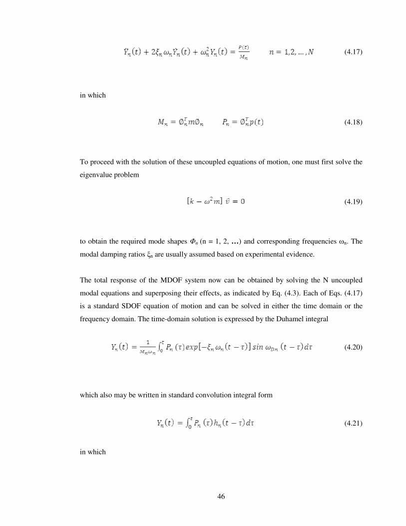
46
(4.17)
in which
(4.18)
To proceed with the solution of these uncoupled equations of motion, one must first solve the
eigenvalue problem
(4.19)
to obtain the required mode shapes Φn (n = 1, 2, …) and corresponding frequencies ωn. The
modal damping ratios ξn are usually assumed based on experimental evidence.
The total response of the MDOF system now can be obtained by solving the N uncoupled
modal equations and superposing their effects, as indicated by Eq. (4.3). Each of Eqs. (4.17)
is a standard SDOF equation of motion and can be solved in either the time domain or the
frequency domain. The time-domain solution is expressed by the Duhamel integral
(4.20)
which also may be written in standard convolution integral form
(4.21)
in which

47
(4.22)
is the unit-impulse response function.
In the frequency domain, the response is obtained from
(4.23)
In this equation, the complex load function Pn(iω) is the Fourier transform of the modal
loading Pn(t) is given by
(4.24)
Also in Eq. (4.23), the complex frequency response function, Hn( ), may be expressed as
follows:
(4.25)
In these functions, and . hn(t) and Hn(i ) are Fourier
transform pairs. Solving Eq. (4.20) or (4.23) for any general modal loading yields the modal
response Yn(t) for t 0, assuming zero initial conditions, i.e., Yn(0) = n(0) = 0. Should the
initial conditions not equal zero, the damped free-vibration response
(4.26)

48
must be added to the forced-vibration response given by Eqs. (4.20) or (4.23). The initial
conditions Yn(0) and Y n(0) in this equation are determined from v(0) and v (0) using Eqs.
(4.6) and (4.7) in the forms
(4.27)
(4.28)
Having generated the total response for each mode Yn(t) using either Eq. (4.20) or Eq. (4.23)
and Eq. (4.26), the displacements expressed in the geometric coordinates can be obtained
using Eq. (4.2), i.e.,
(4.29)
which superposes the separate modal displacement contributions; hence, the commonly
referred to name mode superposition method. It should be noted that for most types of
loadings the displacement contributions generally are greatest for the lower modes and tend to
decrease for the higher modes. Consequently, it usually is not necessary to include all the
higher modes of vibration in the superposition process; the series can be truncated when the
response has been obtained to any desired degree of accuracy. Moreover, it should be kept in
mind that the mathematical idealization of any complex structural system also tends to be less
reliable in predicting the higher modes of vibration; for this reason, too, it is well to limit the
number of modes considered in a dynamic-response analysis.
The displacement time-histories in vector v(t) may be considered to be the basic measure of a
structure's overall response to dynamic loading. In general, other response parameters such as
stresses or forces developed in various structural components can be evaluated directly from
the displacements. For example, the elastic forces fS which resist the deformation of the
structure are given directly by

49
(4.30)
An alternative expression for the elastic forces may be useful in cases where the frequencies
and mode shapes have been determined from the flexibility form of the eigenvalue equation.
Writing Eq. (4.30) in terms of the modal contributions
(4.31)
leads to
(4.32)
Writing this series in matrix form gives
(4.33)
where ω2
n Yn(t) represents a vector of modal amplitudes each multiplied by the square of its
modal frequency.
In Eq. (4.33), the elastic force associated with each modal component has been replaced by an
equivalent modal inertial-force expression. The equivalence of these expressions was
demonstrated from the equations of free-vibration equilibrium; however, it should be noted
that this substitution is valid at any time, even for a static analysis.
Because each modal contribution is multiplied by the square of the modal frequency in Eq.
(4.33), it is evident that the higher modes are of greater significance in defining the forces in
the structure than they are in the displacements. Consequently, it will be necessary to include

50
more modal components to define the forces to any desired degree of accuracy than to define
the displacements.
4.5 Mode Combination
Modal analysis is performed to identify the modes, and the response in that mode can be
picked from the response spectrum. This peak response is then combined to estimate a total
response. A typical combination method is the square root of the sum of the squares (SRSS) if
the modal frequencies are not close.
The displacement, velocity or acceleration vector for each mode is computed from the
eigenvector by using a “mode coefficient”:
(4.16)
where: m = 0, 1, or 2, based on whether the displacements, velocities, or accelerations,
respectively, are selected.
Ai = mode coefficient
The mode coefficient is computed for acceleration excitation of base
(4.17)
where: Sai = spectral acceleration for the ith mode (obtained from the input acceleration
response spectrum at frequency fi and effective damping ratio
γi = participation factor for the ith mode.
The participation factors for a given excitation directions are defined as:
(4.18)
where: γi = participation factor for the ith mode
D = vector describing the excitation direction

51
The modal displacements, velocity and acceleration (Equation 4.16) may be combined in
different ways to obtain the response of the structure. The response includes DOF response as
well as element results and reaction forces.
Only those modes having significant amplitude (mode coefficient) are chosen for mode
combination. A mode having a coefficient of greater than a given value of the maximum
mode coefficient (all modes are scanned) is considered significant.
The combination is done by a generalization of the method of the square root of the sum of
the squares which has the form:
(4.19)
where:
Ra = total modal response
N = total number of expanded modes
εij= coupling coefficient. The value of εij = 0.0 implies modes i and j are
independent and approaches 1.0 as the dependency increases
Ri = AiΨi = modal response in the ith
mode (Equation 4.16)
Rj = AjΨj = modal response in the jth
mode
Ai = mode coefficient for the ith
mode
Aj = mode coefficient for the jth
mode
Ψi = the ith
mode shape
Ψj = the jth
mode shape
Ψi and Ψj may be the DOF response, reactions, or stresses. The DOF response, reactions, or
stresses may be displacement, velocity or acceleration.
For the case of the SRSS (Square Root of the Sum of the Squares) Method, Equation (4.19)
reduces to:
(4.19)

52
Having seen the theory of mathematical modeling of a structure for spectrum analysis in the
next chapter (Chapter Five) we go through the detail of the modeling of the satellite with the
review of design of satellite strictures from literatures.

53
Chapter Five: FE Modeling and Analysis of a Satellite Structure
To get a good understanding and practical experience with the energy limiting method, a
simple satellite structure is modeled, and analyzed. Therefore this section describes the FE
modeling and analysis of a satellite that is devised as a multipurpose bus for scientific
application with the introduction part including the collected information from the literature
to meet the modeling of the satellite.
The modeled structure includes a main body (platform & frame), an adapter, two solar panels
and some instruments that controlled and communicated the satellite. It is overall shape
resembles a hexagonal prism weighting about 1030Kg. The configuration of the satellite is
500 mm in major diameter, and approximately 1050 mm in height. The platforms are
assumed consists of aluminium frames and connected by means of welding. The mission
loads (payloads) are assembled on the top of the honeycomb platforms. The analysis of the
structure is divided into two parts: static and dynamic properties. The static analysis ensures
that the structure can withstand axial inertial g load and support the masses of the payloads
during launch, and the dynamic analysis investigates the stiffness properties and prediction of
notching of the structure for test attachment.
5.1 Introduction
5.1.1 Satellite’s Missions
Satellites provide numerous services for modern society. They perform essential duties for
military, governmental, and commercial organizations. The missions of these spacecraft
include science ventures such as earth observation, interplanetary exploration, astronomy, and
solar physics. They also include commercial endeavours such as television signal
transmission, data transmission, and satellite telephone communication.
The majority of the space science missions are performed by NASA-built spacecraft. The
design and size of these spacecraft are highly dependent on the mission goals. These goals are
constantly evolving due to changes in technology, political agenda, and budget. As a result,
the design and size of satellites reflect these changes. This phenomenon is readily proven by
examining the masses of civilian spacecraft launched throughout history. Figure 5.1 displays
the launch mass of several NASA spacecraft as a function of time. The plot shows a gradual
mass increase until the early 1990s at which point the spacecraft masses suddenly begin to

54
decrease. This sharp decrease is primarily due to the change in policies at NASA towards the
“faster, better, cheaper" program and a decrease in the overall NASA budget. These smaller
spacecraft are inherently less expensive to launch. The subsystems can therefore afford to
take a high risk/low cost approach toward the design and offer less redundancy. This decrease
in redundancy also decreases the overall cost and size of the spacecraft. NASA is now using
constellations or formations of small-satellite systems to perform missions that once required
large multi-million dollar spacecraft.
Figure 5-1 Launch Mass History of NASA Spacecraft
The commercial spacecraft industry has also evolved throughout history, as shown in Figure
5.2. However, the masses have not decreased as significantly due to several factors. A major
factor for this trend is the high gain antennas and large power requirements inherent to the
communications satellites placed in geosynchronous orbit. The communications industry has
long exploited the phenomena of “fixed" geosynchronous spacecraft to provide a stationary
signal to its ground-based antennas. This current practice appears to be changing, however, as
distributed spacecraft systems become more prevalent (eg: XM radio, Globalstar, etc.).

55
As we have shown, the satellite industry has transformed to match the ever-changing
environment of technology. Spacecraft mass, as a result, has also demonstrated this trend.
Figure 5-2 Launch Mass History of Commercial Spacecraft
5.1.2 Satellite Structures
Aerospace structures generally require lightweight designs. The goal of these designs is to
optimize the strength per weight, or efficiency of the design. Satellite structural design has
evolved greatly over the past four decades. Traditionally, efficiency has been accomplished
using a combination of various structural designs and materials. We begin this section by
discussing basic primary structural designs and conclude by presenting traditional materials
used in spacecraft.
5.1.2.1 Conventional Structural Designs
Primary structures are designed using several criteria that depend on the mission
requirements. Conventional spacecraft incorporate four basic primary structural designs: 1)
skin-frame structures; 2) truss structures; 3) monocoque cylinders; and 4) skin-stringer
structures.

56
The skin-frame structural design uses an interior skeletal network of axial and lateral frames
to mount exterior skin panels using fasteners or rivets. The frames support bending, torsional,
and axial forces. The skin reinforces the structure by supporting the shear forces introduced
by the interior member connections. The skin is sometimes minimized to save mass, even
though the thin skin leads to some structural instabilities. When the skin buckles due to shear,
it transfers all additional shear loading to in-plane tension forces at 45o which must be
supported by the connections. The buckling modes of the skin exhibit large deformations that
make it insufficient for exterior mounted components such as solar cells. The buckling
strength of the assembly is typically increased by adding intermediate members.
Truss structures use an array of members that can only support axial loads. Truss members
are produced independently and arranged typically in arrays of triangles for stability. The
members are manufactured using extruded tubes made of composite, metallic, or sheet metal
materials. A stable truss is statically determinate and has no excess members to introduce
alternate load paths. Trusses are generally mass-efficient when the members are configured
into rectangular or triangular cross-sectional assemblies. However, they become less efficient
as the cross-section becomes more circular or hexagonal. Also, the design of the structure
creates inherent stress concentrations at interface mounting points, such as separation
systems. Components may be mounted both internally and externally and the absence of shear
panels enables easy access to a payload. However, this absence of shear panels is not helpful
to spacecraft requiring body mounted solar cells.
Monocoque cylinders are axisymmetric shells that do not contain any stiffeners or frames.
The shells are manufactured using metallic or sandwich panels with curved sections formed
by rolling. Typically, two or three curved sections are fabricated and assembled into the
cylindrical configuration. The strength of monocoque cylinders is usually limited by its
buckling strength. The shells are most efficient when the loads are distributed evenly
throughout the structure. Components are typically mounted to the walls using fasteners;
however, care must be taken not to overload the shell and cause local failures. The
monocoque cylinder design is applicable to spacecraft with body mounted solar cells and
relatively lightweight components.
Cylindrical skin-stringer structures are designed using axial and lateral frame members
attached to an outer skin. These designs are similar to skin-frame structures; however, this

57
class of structures refers to circular cylinder configurations. The skin is sometimes minimized
to save mass, even though the thin skin leads to some structural instabilities. The post-
buckling behaviour of the skin transfers the additionally applied shear loads to torsion by the
diagonal tension phenomenon described above. The skin and members must attach uniformly
to enable the assembly to act as a continuous structure. Typical connection methods include
fasteners and/or rivets. Interior components are usually mounted to the walls at locations
along the stringer assembly. This method is more efficient than monocoque cylinder
component mounting at introducing local loads. The skin must be designed sufficiently stiff
to enable sound mounting of exterior entities such as body mounted solar cells.
5.1.2.2 Materials
Satellite structural designs also use several different materials. Materials are chosen based on
their properties, cost, and complexity. There are two typical materials used in spacecraft.
Metals
Aluminium alloys are the most widely used metallic materials in spacecraft manufacturing.
The advantages include high strength to weight ratios, high ductility and ease of machining.
The stiffness to weight ratio is comparable to steel; however, the strength to weight ratio is
typically higher. The disadvantages include low hardness and a high coefficient of thermal
expansion (CTE). The alloys are typically tempered to increase the material strengths. Two
typical alloys used in manufacturing are 6061-T6 and 7075-T7. Aluminium 6061-T6 contains
silicon and magnesium which strengthens the alloy during tempering. This alloy has good
machinability and corrosion resistance. Aluminium 7075-T7 contains zinc and trace amounts
of magnesium. The alloy exhibits higher strength than 6061-T6, but is more difficult to
machine.
Beryllium is used for very high-stiffness aerospace applications. It has a specific modulus 6.2
times the specific modulus of aluminium. The material is non-isotropic due to its grain
alignment and therefore exhibits low ductility and fracture toughness in its short-grain
direction. It is commonly used in lightweight optics and mirrors because it performs well at
cryogenic temperatures (i.e. low CTE and high thermal conductivity). However, beryllium is
expensive, difficult to machine, and sparsely available in the US. Beryllium must be

58
machined in a controlled environment because its powder is a known carcinogen when
inhaled. The parts may be safely handled once machined.
Steel is mainly used in aerospace applications where low-volume strength and stiffness are
important. Steel provides high wear resistance; however it is generally difficult to machine
and is not efficient for structural stability. Steels are combined with many trace elements to
address a wide range of needs. Austentic stainless steel is by far the most abundant steel alloy
used in spacecraft. It contains 12% chromium which results in a tough chromium-oxide
coating that protects parts from corrosion. Stainless steel is non-magnetic and certain low-
carbon alloys can be welded without sensitization. Stainless steels are generally used for
fasteners and mechanisms whereas many heat-resistant alloys are used for heat shields, rocket
nozzles, and other high-temperature applications.
Titanium and titanium alloys are used for applications requiring very high strength materials.
The materials exhibit high strength to weight ratios, low coefficients of thermal expansion,
and excellent corrosion resistance. However, they are difficult to machine and some alloys
exhibit poor fracture toughness. Ti-6Al-4V, which contains 6% aluminium and 4% vanadium,
is the most popular titanium alloy used in aerospace applications. The alloy has heritage in
wings and missile bodies. Perhaps its most famous applications are the castings used to
connect the external fuel tank to the Space Shuttle and its boosters.
Fiber Composite Structures
Composite structures consist of a matrix and reinforcement. The matrix (metal, epoxy) binds
the reinforcing fibers (carbon, graphite) together into a continuous system. The efficiency of
composite structures is due its high specific modulus and unique load path. The flexural shear
loads are transferred from the matrix to axial loads on the high-strength fibers, creating a
structure 3 to 5 times as stiff as aluminium at 60% of the mass. These fibers may be both
discontinuous and continuous entities. Discontinuous-reinforced composites are comprised of
ceramic or fiber particles that are randomly distributed throughout the matrix. Aluminium
reinforced with silicon carbide particles is the most widely used discontinuous composite.
The majority of continuous-fiber composites are generally called laminate composites.
Laminate composites are manufactured from several layers of woven fibers called laminae.
The laminae are composed of several parallel fibers arranged in sheets. The sheets themselves
are anisotropic and have few structural applications. However, stacking several of the laminae

59
with fibers aligned at different angles, called lamina angles, creates a more stable laminate
composite structure. The laminate may be customized for individual applications by varying
the fiber type and the lay up. For example, some graphite/epoxy laminates are tailored to have
a nearly zero CTE and others may be laid up to exhibit extraordinary specific stiffness
properties. Polymer-matrix composites (PMCs) are the most widely used continuous-fiber
composites used for spacecraft. The matrices consist of two polymers: thermoplastics, and
thermosets. Thermoplastics may be remelted and solidified multiple times whereas
thermosets are not reusable after curing. These properties enable a multitude of bonding
techniques and lay up procedures, many of which are currently proprietary. The downside to
fiber composite structures is the large development cost required for reliable manufacturing.
The large cost is due to the sensitivity of adhesive bonding to process variables. This
sensitivity makes each part a unique entity which must be tested to verify strength. NASA and
other programs require extensive testing of fiber composite flight hardware to verify its
structural integrity. The requirements typically create the need to fabricate a protoflight
structure dedicated to qualification testing followed by acceptance testing of the flight article.
This qualification procedure presently prohibits the use of fiber composite structures on
small-budget programs.
5.1.3 Structural Optimization Methods
Several methods are available to optimize the structural properties of spacecraft. The
optimum method may vary depending on the design task. We present three of the most widely
used methods: sandwich structures, multifunctional structures, and isogrid. We examine all of
the technologies and their benefits for satellite structural designs. We conclude with a
description of isogrid and a literature review of past research conducted in this field.
Sandwich Structures
Sandwich structures are often used in skin-frame designs. A sandwich structure consists of
two thin face sheets attached to both sides of a lightweight core. The design of sandwich
structures allows the outer face sheets to carry the axial loads, bending moments, and inplane
shears while the core carries the normal flexural shears. Sandwich structures are susceptible
to failures due to large normal local stress concentrations because of the heterogeneous nature
of the core/face sheet assembly. Component mounting must therefore use potted inserts to
distribute the point loads from connections. Sandwich panel face sheets are commonly

60
fabricated using aluminium or graphite/epoxy composite panels. The core is typically
fabricated using a honeycomb or aluminums foam construction.
Honeycomb sandwich paneling is the lightest option for compressive or bending loading
specific applications. Honeycomb sandwich cores are manufactured using thin strips formed
into honeycomb cells. The honeycomb geometry is non-isotropic with greater stiffness in the
longitudinal direction. However, the core acts nearly isotropically for in-plane loads when
assembled in a sandwich configuration. The disadvantages of using honeycomb cores are the
potted inserts required for mounting and the thermal inefficiencies. These inefficiencies stem
from the low thermal conductivity of the adhesive layers used in construction and make
honeycomb prohibitive in optical and mirror aerospace applications.
Aluminium foam sandwich panels use a porous aluminium foam material for the core. The
flexural shear stiffness dominates the overall panel stiffness for relatively small panels (i.e.
less than 50 inches). Therefore, the core design is an integral part of the sandwich panel
design for small spacecraft. The shear stiffness of foam core sandwich panels is generally less
than that of honeycomb core sandwich panels of equal mass. However, radial ribs and shear
rings may be embedded in the core to overcome the low shear stiffness. A major benefit of
aluminium foam construction is an increase in thermal efficiency because the core may be
brazed to aluminium face sheets rather than epoxied. Brazing provides a continuous thermal
path through the material which benefits applications such as cryogenic mirrors and solar
arrays.
Multifunctional Structures
Multifunctional structure (MFS) technology incorporates several functions into the primary
structure of a spacecraft. The main goal of these members is to minimize parasitic mass by
incorporating chassis, cables, connectors and thermal control components into the satellite
primary structural walls (see Figure 5.3). The walls are typically constructed out of fiber
composites or sandwich panels, and the electrical components are embedded during
manufacturing. The traditional ground plane/printed circuit board design is performed by
copper/polymide (CU/PI) patches, multi-chip modules (MCMs), and the current cabling
functions are performed using CU/PI flexible jumpers. The design allows for an easily
accessible, removable, and modular electrical system [13]. The benefits of this technology
include a 70% reduction in electronic

61
Figure 5-3 Schematic of MFS Configuration
enclosures and harnesses, a 50% reduction in space craft volume required for these
conventional components, a reduction in labour required for spacecraft assembly, and an
extremely robust system with wide applicability to several missions. Lockheed Martin has
recently proven the technology as an experiment aboard the Deep Space 1 mission.
5.1.3.1 Isogrid Structures
Isogrid uses an array of equilateral triangle cut outs to increase the stiffness per weight of a
structure. The pattern may be manufactured by machining a metallic panel, or it may be
constructed using fiber composite materials. The concept began in the early 1960s using
metal structures and development continues today with research focusing primarily on
composite applications.
5.2 FE Model Generation of the Satellite
To reach the stated objective of this practical phase of the project, design criteria for the
satellite structure was defined. These criteria included
• Significant over testing must be present,
• The natural frequencies should be in the 2-60 Hz frequency range,
• The test structures should be easy to analyze,
• The acceleration environments should be within the acceptable specification of the
test shaker.

62
Structural Configuration
The Satellite structural configuration is designed to accommodate all of the mission
components or payloads (Figure 5.4). The structural assembly consists of ten plates. The two
end panels are hexagonal plates measuring 50 mm in major diameter and 4 mm in thickness.
The two payload panels are hexagonal honeycomb plates measuring 6 mm in thickness. The
side panels are formed using 2.5 mm thick plates. The frames reinforce the side panels and
solar panels which measure 1500X500X4 mm and provide a stiff, stable surface to affix solar
cell arrays.
Figure 5-4 Geometry model of the satellite model

63
5.2.1 Geometry Modeling
Figure 5.4 is a drawing of the Satellite that was built. The geometry for a Satellite was created
on ANSYS by defining key points, lines, areas, volume.
The Satellite is made of many thin structures, which is defined as area in the model and frame
structure, which is defined as line. Some of the secondary structures, such as the propulsion
module is defined as a sphere volume attached with a ring to the lower platform and scientific
payloads are defined as a key point attached with the supporting beam structure on the
honeycomb platform. The model will be initially broken up into seven groups, each
representing a separate piece of the structure. These groups include: lower platform, upper
platform, honeycomb platform, solar panels, adapter cone, side panels, central cylinder, and
frame geometry.

64
Figure 5-5 Geometry specifications for the Satellite (dimensions are in mm).
5.2.2 Finite Element Model
In this section, it is defined a finite element mesh for the Satellite model that was developed
earlier.
First material property is defined by creating Isotropic materials, named titanium and
aluminium, which uses a Linear Elastic Constitutive Model. The material’s Elastic Modulus,
Poisson’s Ratio and Density are 110.4 GPa, 0.16, 7474 Kg/m3, and 72.45 GPa, 0.33, 2796
Kg/m3, respectively.

65
Then the element type and real constants are defined for idealizing the different components
of the satellite. Therefore for the thin structures such that the lower and upper platforms are
idealized as a plate element. The scientific platform is a honeycomb structure which is
idealized as a plate element by calculating the equivalent thickness of the plate given by eqn.
(5.1)
(5.1)
where is the equivalent thickness of the plate
is the Poisson’s Ratio of the honeycomb
is the moment of inertia of the honeycomb
The scientific payloads of the satellite model are idealized as concentrated masses. The
concentrated masses will be modeled with Point Elements. It is also applied a rigid element to
model propulsion module.
The real constants will include properties for 2-D shell elements, 1-D frames, 3-D solid, and
0-D concentrate masses and the assignemet of the material properties for the components is
shown in table 5.1.
Additionally, it is created a field to define a thickness variation in the Adapter cone. The
thickness of the cone will be 5 mm at its base and will vary linearly to a thickness of 10 mm
at its top dimension as shown in fig. 5.6.

66
Figure 5-6 Adapter Cone’s specifications - 2D slice (dimensions are in cm)
Component Material type Real constant Material
Central cylinder Shell 63 T = 4 mm Aluminium alloy
Adapter Shell 63 T = 5-10 mm Titanium alloy
Upper platform Shell 63 T = 2.5 mm Aluminium alloy
Lower platform Shell 63 T = 4 mm Aluminium alloy
Honeycomb platform Shell 63 T = 6 mm Aluminium alloy
Side panels Shell 63 T = 2.5 mm Aluminium alloy
Solar panels Shell 63 T = 4 mm Aluminium alloy
Propulsion block Solid 164 m = 360 Kg Aluminium alloy
Payloads Mass 21 m = 640 Kg Aluminium alloy
Payloads supporting
beam
Beam 4 Hollow box
50X50X2.5 mm
Aluminium alloy
Main structure frame Beam 4 Angle iron
50X50X2.5 mm
Aluminium alloy
Solar panel frame Beam 4 Angle iron
40X40X2.5 mm
Aluminium alloy
Table 5.1 The Element Property assignments
Finally the model is meshed: first by attributing element types, real constants and material
properties to the geometric model; then by setting mesh size control and generating the mesh.
Note that to attain connectivity between the nodes of different elements it has been made all
the elements to have the same Degree Of Freedom (DOF) and each node to overlap.

67
5.3 Defining Boundary Condition
It is assigned Boundary conditions to the model and set up two boundary conditions; launch
and test attachment for the loading conditions of dynamic analysis and Static analysis
respectively.
A simply supported displacement constraint, named Launch constraint (used for static
analysis), for all vertices on the outside edges of the Upper and Lower Platforms (i.e., ball
joint) is created. The displacement is fixed in translation and free in rotation. Test constraint
(used for dynamic analysis) is made by a fixed support displacement constraint by setting
zero in translation and rotation for all vertices on the outside edges of only the lower
platforms.
Finally, it is defined two Load Cases for this model. One Load Case contains only the Launch
constraints and is use for static analysis. Another Load Case contains the Test constraints
meant for the dynamic analysis.
5.4 Static and Spectral Analysis of the Satellite
5.4.1 Static Analysis
Static analysis is done for an inertial loading created due to the launch accelerations. It is
defined a loading, of 14g load in the Z direction. It should be noted, the gravity constant for
this problem is 1 g = 9.81 and the inertial loading is applied to the entire model.
5.4.2 Spectral Analysis
Spectral analysis is done for a test condition of swept test where the excitation is in the form
of a sinusoidal except that the frequency and magnitude are varied slowly. The frequency is
swept slowly from a low frequency 2 Hz to an upper frequency limit, between 4 and 40Hz
and in the downward direction up to 60 Hz. Constant peak accelerations between 1g to 14g is
applied as shown in figure (5.7) below. To apply these dynamic loads spectral analysis is
done.

68
Figure 5-7 Curve Showing the Input versus Forcing Frequency
A single-point response spectrum (SPRS) analysis is used because, we specify one response
spectrum curve (or a family of curves) at a set of points in the model, such as at all supports,
as shown in Figure (5.8).
Figure 5-8 Single-Point Response Spectra
The procedure for a single-point response spectrum analysis after building the model consists
of five main steps:
1. Obtain the modal solution.
2. Obtain the spectrum solution.
3. Expand the modes.

69
4. Combine the modes.
5. Review the results.
Obtain the Modal Solution
To determine natural frequencies normal mode analysis is done. The standard Block Lanczos
algorithm available in ANSYS is used, which extracts the required eigenvalues of a matrix.
The number of modes extracted should be enough to characterize the structure's response in
the frequency range of interest.
Obtain the Spectrum Solution
ANSYS offers the Single-point Response Spectrum (SPRS) for a spectrum analysis. Not all
modal analysis options and not all eigenvalue extraction techniques work with all spectrum
analysis options.
Enough modes to cover the frequency range spanned by the spectrum and to characterize the
structure's response were chosen. The accuracy of the solution depends on the number of
modes used: the larger the number, the higher the accuracy
Spectrum type is acceleration and the Excitation Direction is in the Z coordinate. Spectral-
Value-Versus-Frequency Curve of figure 5.6 is applied.
The output from the solution includes the participation factor table. The participation factor
table, which is part of the printed output, lists the participation factors, mode coefficients
(based on lowest damping ratio), and the mass distribution for each mode. To obtain the
maximum response of each mode (modal response), multiply the mode shape by the mode
coefficient. We can do this by retrieving the mode coefficient with the GET command and
using it as a scale factor in the SET command.
Expand the Modes
Then mode expansion as a separate solution pass after performing the spectrum solution was
performed. It is used to selectively expand (write mode shape to the result file) significant
modes. Only expanded modes are used for the mode combination operation in the subsequent
mode combination pass.

70
It expands only those modes whose significance level exceeds the SIGNIF threshold. The
significance level of a mode is defined as the mode coefficient of the mode, divided by the
maximum mode coefficient of all modes. Any mode whose significance level is less than
SIGNIF is considered insignificant and is not expanded. The higher the SIGNIF threshold, the
fewer the number of modes expanded. Therefore a SIGNIF 0.001 is taken for this problem.
Combine the Modes
ANSYS offers five different mode combination methods for the single-point response
spectrum analysis. But Square Root of Sum of Squares (SRSS) is used. These combine the
maximum modal responses by using the specified mode combination method to calculate the
overall response of the structure.
Review the Results
Results from a single-point response spectrum analysis are written to the mode combination
file. These commands calculate the overall response of the structure by combining the
maximum modal responses in some fashion (specified by one of the mode combination
methods).
The next chapter describes a detailed result of the static and dynamic analysis of the case
study for a specific satellite, an analytical method of the notch predictions are conducted
followed by the result of the ANSYS.

71
Chapter Six: Results of Static and Dynamic Analysis
This chapter contains plots of the stress contours obtained in the static and dynamic test finite
element analysis. Both the shell stresses and beam stresses are plotted. The results shown are
the Von-Mises stresses and the total displacements calculated in the analysis. Keep in mind
that the unit of all the ANSYS results now on wards are in SI units.
The mesh shown below is the frame of a satellite modeled as beam and plate elements,
specifically consisting of 7140 elements and 6009 nodal points. The structure optimum
weight has been calculated equal to 1031 kg.
Figure 6-1 FE Model of the Satellite
6.1 Static Analysis
In the static analysis, 14g inertia load has been applied on the satellite model in the axial
direction, and the end corners of the upper and bottom platform have used as fixed points
only for translation for boundary condition of launcher attachment. After several runs, the
optimum value for the discussed geometric parameters has been finalized with a safety factor

72
equal 4 for the maximum von-mises stress of 54.7 MPa and yield strength of the material is
200 MPa. Therefore the structure is found safe where the margin of safety for satellite
structure is 1.05. The highest stress value is observed in the side panels where the connections
of the solar panels’ frames are made (fig.6.2).
Figure 6-2 Total Displacement Stress in the Space Satellite

73
Figure 6-3 Von-Mises Stress in the Space Satellite
6.2 Modal Solution of Vibration Test
The goal of modal analysis is to determine the natural shapes and frequencies of the structure
during free vibration and to determine the response of a structure due to dynamic loads. This
modal approach is popular due to its efficiency and can approximate the response using only
a small number of modes. When dealing with small models all the modes in the frequency
range of interest are included for the response solution. But for larger structures, including all
the modes in the frequency range can be computationally expensive. Therefore it is important
to understand the modes with large contributions to the overall response of the structure.
The first step in calculating the modal frequency response is to compute the normal modes of
the structure. The results from the normal modes analysis are the mode shapes and natural
frequencies. Observing the mode shapes reveals how the structure will deform at natural
frequencies. However, the modal displacements / deformation information does not provide a

74
good insight to the response since the Eigenvectors are arbitrarily scaled and the
displacements seen in the postprocessor can be deceiving.
The next images are that of the 4 modes of this satellite during free vibration. This problem
can be seen as a depiction of the likeliest deflections a satellite would take during a base
excitation; since in most satellite the first four modes preferably used. As expected, the first
mode is a swaying of the satellite panels from up to down. The second, mode is swaying of
the honeycomb platform. The third mode is the swaying mode of the adapter cone. The fourth
mode is a stretching and compression mode in the vertical z direction.
Figure 6-4 Swaying Front to Back of the Solar Panels

75
Figure 6-5 Swaying of the Honeycomb Platforms
Figure 6-6 Swaying of the Adapter Cone

76
Figure 6-7 Drum Type Mode
The modal effective mass associated with each deformation mode represents the amount of
system mass participating in that mode. Therefore, a mode with a large effective mass is
usually a significant contributor to the system’s response. These criteria are in other words
used to find the important system modes. A typical requirement for the selection of target
modes is that modes with a translational effective mass equal to or greater than 2 percent of
the total mass are target modes.
The normal modes analysis is performed for a frequency range of 2 Hz to 60 Hz. The modal
effective mass can be printed out during the normal modes solution. A trial run is conducted
to determine the number of modes needed to represent the response of the entire structure.
One way to determine this is to calculate the cumulative modal effective mass. If the
cumulative sum of modal effective mass is more than 80%, then the modes are sufficient to
represent 80% of the response of the structure. In some applications, the requirement is to use
95%. The modal effective mass table is printed out along the direction of the excitation as
shown in table 1. The sum along the direction should be compared with the total mass of 1030
Kg.

77
The results of the analysis are shown in table 1 and figure 1. It can be seen that modes 4,
9,10,12,31 and 64 represents 97 % of the response in Z direction. A quick review of the table
reveals that, for most applications it is just sufficient to consider the first 64 modes of the
structure to simulate the frequency response of the entire structure.
mode frequency
participation
Factor
Modal
effective mass
mode
coefficient
percentage
contribution
4 3.183 3.615 13.06823 5.302 1.2675291
9 20.03 -8.177 66.86333 -7.23E-03 6.4852889
10 20.04 -1.017 1.034289 -8.98E-04 0.100319
12 20.73 -0.09637 0.009287 -7.95E-05 0.0009008
31 28.77 -16.7 278.89 -7.16E-03 27.050436
64 57.72 25.3 640.09 6.69E-04 62.084384
Table 6.1 Modal Effective Mass
Figure 6-8 Modal Contributions in the Z Translation (for the chosen input load)
6.3 Dynamic Analysis
This section presents the dynamic response produced by the test item during the test
configuration. It is important to note that this configuration is completely used to study the
phenomena of the response of the satellite by producing the boundary condition of rigid
shaker table’s fixture and predict the critical places and notch value using energy limiting
method.
Mode Number

78
A complete dynamic structural analysis of the test structure was performed. The analysis
started with a modal analysis where natural frequencies, the effective masses were computed
for the satellite structure as stated in the above section. Then the analysis continued with the
base-driven sinusoidal vibration analysis of the test system. This analysis is a representation
of the real-life condition of test. It yields the von-mises stress of the satellite, which
corresponds to the test condition of the satellite.
6.3.1 Critical Location Prediction
One or more critical Locations on the satellite for vibration testing are predicted from the
response of von-mises on the nodes with a maximum stress for a specific frequency. It is
quite clear that those fundamental (resonance) frequencies are with a peak stress value than
other frequencies. Therefore for each fundamental natural frequency the node with the most
pike von-mises stress value is taken as critical location and seen for the spectral response.
For the satellite, the dynamic base excitation that is shown in chapter 5 is utilized. The
material being alloy-aluminium, we can use the “Von-mises theory of failure”. So the stresses
are obtained as the von-mises stresses.
Fig. 6.9 shows von-mises stress variation for nodes taken as critical location and lists the
nodes with their numbers consistently to ANSYS results to locate the locations on the satellite
model. Each location represents the node with maximum von-misses stress for the
fundamental resonance frequencies which have higher participation as stated in above section
such that 3.18, 20.03, 20.04, 20.73, 28.766 and 57.72 Hz and the respective nodes are 799,
344, 85, 3611, 629, 332 and their relative location on the model is shown on fig. 6.1. It can
be seen from the relative comparison of curves of the graphs that, the stresses are maximum
for node 3611 which is located at the lower honeycomb panel. For this node the peak stress
within 60 Hz is 1790 MPa at resonance frequency of 20.73 Hz while the stresses induced at
all elements are found absolute peak. The 4th
node thus is the most critical point out of the six
nodes.

79
Figure 6-9 Maximum Stresses Induced for Node no. 799, 344, 85, 3661, 629 and 332
6.3.2 Notch Value Prediction Using Energy Method
For this satellite structure, only the notching of the critical elements, where the critical nodes
are founded, is of interest, since these elements by far are the dominant one to predict the
notch value. Also the strain energy value of the von-mises stress is a prime important
parameter since it is related to the total amount of energy transmitted to the test item during
the vibration test.
The strain energy at the critical element during test was determined from the von-mises
stresses with the following assumption: when an element is subjected to a resultant stress due
to some load the element is strained and the work done by the external applied load must be
stored up in the element in the form of strain energy. The strain energy U will be given on a
differential volume dv by:
(6.1)

80
Where is the von-mises stress and
is the strain.
If the element has constant cross sectional thickness t and volume v, then
dV = t dA
and we have the relation (6.2)
and substituting Eqns. (6.2) into eqn. (6.1) yields
(6.3)
While the element shape is assumed as a rectangle as shown below.
Figure 6-10 Rectangular Element
The von-mises stress can be assumed to have a form of polynomial function of x and y
variables over the element like
( ) xyayaxaayxv 3210, +++=σ (6.4)
after solving it will be

81
( )( ) ( ) ( )
xyab
yb
xa
yx vvvvvvvv
vv
43211412
1,σσσσσσσσ
σσ−+−
+−
+−
+= (6.5)
This equation will be inserted into eqn. (6.3) to estimate the strain energy applied to the
element and solving the double integral. Note that the detail derivation of all the equations in
this section is shown in Appendix A.
Finally, energy specifications can be defined. The specification for energy is determined by
substituting the stresses with the yield stress of the material to eqn. (6.3). Therefore the
notching values for the elements of critical locations are shown in the table 6.2.
Elements of
critical locations
Applied strain energy
to the element (J)
Specific strain energy
of the element (J)
Scale of notching
1st 2.225 0.216 10
2nd
3.105 0.216 14.4
3rd
3.105 0.216 14.4
4th
14.99 0.518 30
5th
17.21 1.38 12.5
6th
19.23 1.38 14
Table 6.2 Predicted Notching Value for the Critical Elements
Note that the detailed calculations of notch value of each critical element are shown in
Appendix B.
Therefore we can conclude from the result that with energy limiting, the energy value of the
von-misses stresses of the critical section of elements are reduced by a scale of up to 30 with
a maximum of notching at a resonance of 20.733 Hz. The analysis showed that the energy
specifications will significantly reduce the over testing according to the result accomplished.
The result of the von-mises stress from a single-point response spectrum analysis is shown in
figure 6.10 and the peak stress is 537 Mpa and it is found at the most critical location of the
4th
element. The plot is called a response spectrum of the stress which is simply a plot of the
peak or steady-state response.

82
Figure 6-11 The Overall Von-Mises Stress Contour Plot for the Spectral Analysis
6.4 Verification of the Method
In this section it is considered the simple vibratory system of launch configuration of Figure
6.12, which consists of two oscillators connected in series. The main oscillator is vibrated
through motion of its rigid base; the secondary oscillator is excited because of its attachment
to the main one. To use terminology consistent with literatures, for example, Scharton [41],
the main oscillator is referred to as the source and the secondary oscillator is the load.
Figure 6-12 Source and Load Oscillator in Launch Configuration.

83
The verification of the energy limiting method when compared with the force limiting method
is studied by assuming that the oscillatory system of Figure 6.12 represents a vibration mode
of a flight-mounting structure (source) coupled with a vibration mode of the test article (load).
For this project the mounting structure is a launch vehicle and the test article is the satellite.
As a numerical example, assume that the mass m2 is twice m1, the damping coefficient C of
both oscillator is 30 N Sec/m (i.e., damping ratio of 2.5%), and the spring constant K of both
oscillator is 36E6 N/m. For the launch configuration the same procedure of ANSYS is
followed except that the masses are idealized as a point by an element type of MASS21 and
the spring-damper is idealized as a line by using an element type of COMBIN14.
The amplitude of the coupled system interface acceleration is shown in Figure 6.13. One may
observe the two peak accelerations at the system resonance frequencies located at 18 and 48
Hz. The notch in the interface acceleration at the resonance frequency of 48 Hz is clearly
visible
Figure 6-13 Coupled System Interface Acceleration and Test Specification.

84
The interface force in a coupled system (or flight configuration) is obtained by an analysis as
shown in Figure 6.14. This curve also peaks at the two resonance frequencies of the coupled
system, with a maximum value of 1500 KN occurring at 48 Hz.
Figure 6-14 Coupled System Interface Force.
Figure 6.15 presents the reaction force produced by the test article during the test. The
reaction force peaks at 57.3 Hz, with a value of 3400 KN.

85
Figure 6-15 Reaction Force during Vibration Test.
A comparison of the above peak forces at the coupled system and test configurations shows
that vibration testing with a traditional enveloping method (without response notching) results
in a reaction force during the test that is 2.3 (or 3400/1500) times higher than at the coupled
system level. With FLV, the input acceleration at the test article resonance frequency would
be notched to reduce the shaker force by a scale of 2.3 to the value of 1500 KN, which is the
maximum force produced at the coupled system level.
However energy in a test configuration is obtained and the stress peaks at one of the
resonance frequency of the test system, occurring at the bottom platform taking place at
28.766 Hz. This also shows a notch value of 12.5 which is quite greater to 2.3 value of the
FLV at the support.
It may be noted that our method gives a conservative value which is acceptable. This five
times order of magnitude of conservatism in our engineering procedure is mainly due to the
simplified text book example of modeling of the system made in the case of prediction of
couple interface force.

86
Chapter Seven: Discussion and Conclusions
In this chapter a general discussion on the results is presented, the important conclusions are
listed and some suggestions for further investigations are given.
7.1 Observations and Discussion
The work presented mainly concerns with vibration over testing problem alleviation method
by energy limiting vibration approach. The force limiting vibration method is very similar to
that of energy limiting but the complexity of the method is much more.
7.2 Conclusions
In spite of the many successful applications of force limiting, a number of interesting research
problems remain. Some problems of current interests are: obtaining flight vibratory force
data for validation of the technique, calculating and measuring moment impedances,
combining multipoint impedances, and assessing errors associated with force measurements.
Therefore the following conclusions can be drawn from the present study in an effort to
evolve a new and better method.
• ANSYS is effective software and has analytical techniques to predict the vibratory
flight energy limits based on the acceleration specification.
• The analysis of the satellite structure confirmed that the energy limiting vibration
method is comparative with other methods while significantly notch the amount of
over testing. For the analysis a reduction of the response energy with a scale of up to
30 was achieved.
• The energy limiting minimizes the risk of over testing and the associated failures, cost
penalties, and schedule delays. In addition, more and better science can be flown for
fixed costs, because the hardware need not be over designed for artificial tests.
• The energy prediction depends less or not at all on the flight data and experiments.
First, since the energies at critical points are predicted based on von misses stress, thus
they can be predicted analytically with more confidence since it is safe from structural
failure.

87
• The strain gauges to measure the stresses in vibration tests are commercially available
and make the method easy to apply because it can be put in every critical place
regardless of its accessibility.
• The conventional vibration controllers can be conveniently used for energy limiting.
• Although this work was aimed at the evaluation of the method for its application to
space satellite, it is clear that the same conclusions apply to a whole range of
hardware.
7.3 Suggestions for Future Work
Some of the suggestions for further investigations are:
• To see the application of energy limiting to random vibration testing weather it is
straight forward and beneficial for minimizing over testing of the test item.
• To verify the method through an experiment in a controlled laboratory set up to see its
ease of application and effectiveness to notching.
• To check the method for composite structure.
• And to make parametric study for the shaker table to get the specimen specific
calibration used for the correction of test result.

88
Appendix A. Derivation of Notch Value for an Element
Stress distribution over a rectangular element is as shown it fig. A.1
Figure A.1 stress distribution over an element
Assuming a polynomial function of variables x and y
A.1
For (x,y) = (0,0) we have
Therefore
A.2
And for (x,y) = (a,0) we have
Substituting eq. (A.2) into it and solving it will be
A.3

89
And for (x,y) = (0,b) we have
Substituting eq. (A.2) into it and solving it will be
A.4
And for (x,y) = (a,b) we have
Substituting eq. (A.2), (A.3) & (A.4) into it and solving it will be
A.5
Substituting eq. (A.2), (A.3), (A.4) & (A.5) into (A.1) it will be
A.6
Therefore the applied strain energy to the element is
A.7
But the specific strain energy is by substituting the yield stress for the stresses, so it will be
A.8
It is assumed that the overall reduction in input energy of the shaker table to the test item
during testing can be estimated by calculating for the single element.
Therefore the scale of notching is:
A.9

90
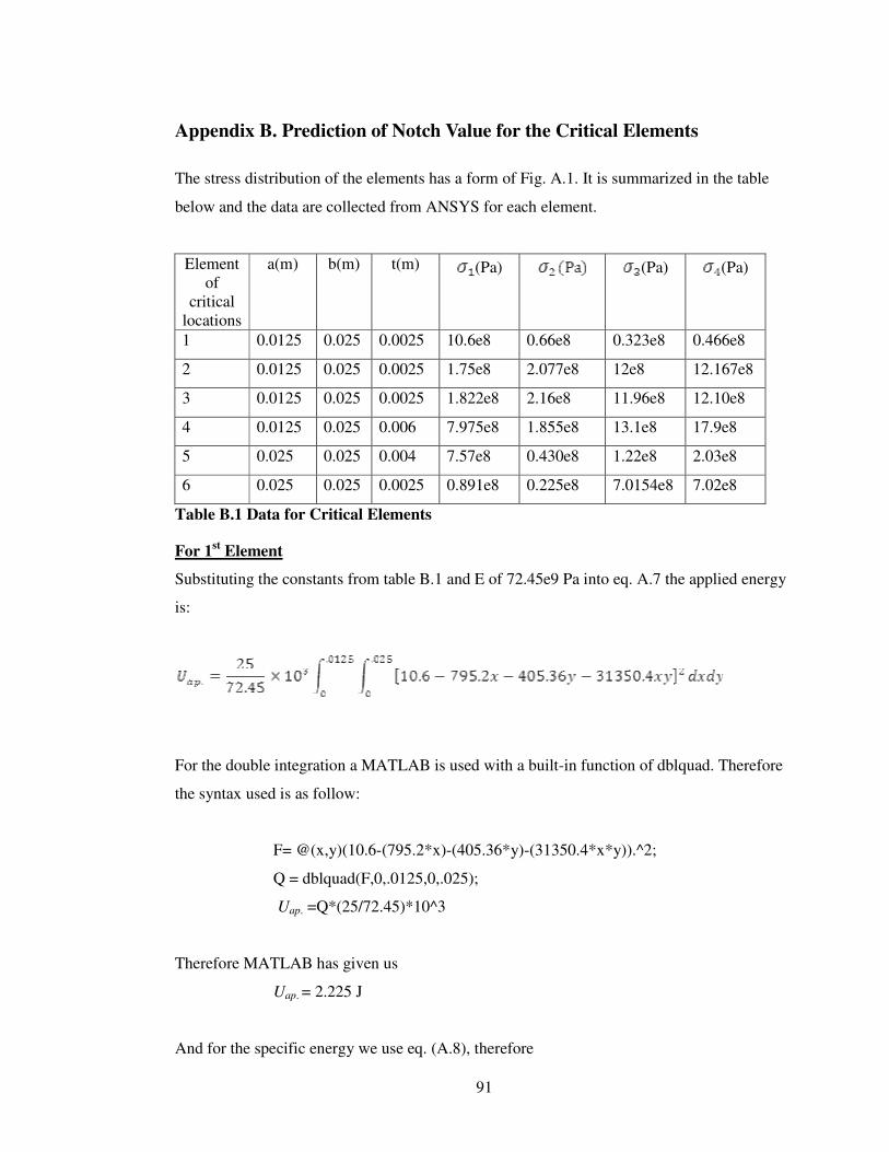
91
Appendix B. Prediction of Notch Value for the Critical Elements
The stress distribution of the elements has a form of Fig. A.1. It is summarized in the table
below and the data are collected from ANSYS for each element.
Element
of
critical
locations
a(m) b(m) t(m) (Pa)
(Pa) (Pa)
1 0.0125 0.025 0.0025 10.6e8 0.66e8 0.323e8 0.466e8
2 0.0125 0.025 0.0025 1.75e8 2.077e8 12e8 12.167e8
3 0.0125 0.025 0.0025 1.822e8 2.16e8 11.96e8 12.10e8
4 0.0125 0.025 0.006 7.975e8 1.855e8 13.1e8 17.9e8
5 0.025 0.025 0.004 7.57e8 0.430e8 1.22e8 2.03e8
6 0.025 0.025 0.0025 0.891e8 0.225e8 7.0154e8 7.02e8
Table B.1 Data for Critical Elements
For 1st Element
Substituting the constants from table B.1 and E of 72.45e9 Pa into eq. A.7 the applied energy
is:
For the double integration a MATLAB is used with a built-in function of dblquad. Therefore
the syntax used is as follow:
F= @(x,y)(10.6-(795.2*x)-(405.36*y)-(31350.4*x*y)).^2;
Q = dblquad(F,0,.0125,0,.025);
Uap. =Q*(25/72.45)*10^3
Therefore MATLAB has given us
Uap. = 2.225 J
And for the specific energy we use eq. (A.8), therefore

92
Therefore the notch scale will be
= 10
Note that the same procedure is used and table 6.2 is produced.

93
References
1. Blake, R. E., “The Need to Control the Output Impedance of Vibration and Shock
Machines”, Shock and Vibration Bulletin, No. 23, June 1956, pp. 59–64.
2. Morrow, C. T., “Application of Mechanical Impedance Concept to Shock and
Vibration Testing”, Los Angeles, CA, TRW Report AD 608030, 1960.
3. O’Hara, G. J., “Mechanical Impedance and Mobility Concepts”, J. of the Acoust. Soc.
Am. 41(5), 1967.
4. Rubin, “Mechanical Immitance and Transmission-matrix Concepts”, J. Acoust. Soc.
Am. 41(5), 1967.
5. Ratz, A. G., “An Impedance Compensated Random Equalizer”, Proceedings of the
Institute of Environmental Sciences 12th Annual Technical Meeting, San Diego, April
1966, pp.353–357.
6. Scharton, T. D., “Development of Impedance Simulation Fixtures for Spacecraft
Vibration Tests”, Shock and Vibration Bulletin, No. 40, Pt. 3, 1969, pp. 230–256.
7. Martini, K. H., “Multicomponent Dynamometers Using Quartz Crystals as Sensing
Elements”, ISA Transactions, Vol. 22, No. 1, 1983.
8. Salter, J. P. , “Taming the General-Purpose Vibration Test”, Shock and Vibration
Bulletin, No. 33, Pt. 3, March 1964, pp. 211–217.
9. Heinricks, J. A., “Feasibility of Force-Controlled Spacecraft Vibration Testing Using
Notched Random Test Spectra”, Shock and Vibration Bulletin, No. 36, Pt. 3, Jan.
1967.
10. McCaa, R. and Matrullo, M. “Flight Level Vibration Testing of a Lifting Body
Reentry Vehicle”, Shock and Vibration Bulletin, No. 36, Pt. 3, Jan. 1967.
11. Painter, G. W., “Use of Force and Acceleration Measurements in Specifying and
Monitoring Laboratory Vibration Tests”, Shock and Vibration Bulletin, No. 36, Pt. 3,
Jan. 1967.
12. Murfin, W. B., “Dual Specification in Vibration Testing”, Shock and Vibration
Bulletin, No. 38, Pt. 1, 1968.
13. Witte, A. F. and Rodeman, R., “Dual Specification in Random Vibration Testing, an
Application of Mechanical Impedance”, Shock and Vibration Bulletin, No. 41, Pt. 44,
1970, pp. 109–118.

94
14. Hunter, N.F. and J. V. Otts, “The Measurement of Mechanical Impedance and Its Use
in Vibration Testing”, Shock and Vibration Bulletin, No. 42, Pt. 1, 1972, pp. 79–88.
15. Witte, A. F., “Specification of Sine Vibration Test Levels Using a Force-Acceleration
Product Technique”, Shock and Vibration Bulletin, No. 41, Pt. 4, 1970, pp. 69–78. B-
2
16. Wada, B. K., R. Bamford, and J. A. Garba, “Equivalent Spring-Mass System: A
Physical Interpretation”, Shock and Vibration Bulletin, No. 42, Pt. 5, 1972, pp. 215–
225.
17. Sweitzer, K. A., “A Mechanical Impedance Correction Technique for Vibration
Tests”, Proceedings of the Institute of Environmental Sciences 33rd Annual Technical
Meeting, 1987, pp. 73–76.
18. Judkins, N. J. and S. M. Ranaudo, “Component Internal Vibration Response
Accelerations—System Level versus Component Level”, Proceedings of the 10th
Aerospace Testing Seminar, 1987, pp. 97–104.
19. Piersol, A. G. , P. H. White, J. F. Wilby, P. J. Hipol, and E. G. Wilby, “Vibration Test
Procedures For Orbiter Sidewall-Mounted Payloads: Phase I Report Appendices”,
Astron Research and Engineering (Santa Monica, CA), Rept. 7114-01, 1988.
20. Scharton, T. D. and D. L. Kern, “Using the VAPEPS Program to Support the TOPEX
Spacecraft Design Effort”, Proceedings of the 59th Shock and Vibration Symposium,
1988, pp. 21–36.
21. Scharton, T. D., Boatman, D. J. and Kern, D. L., “Dual Control Vibration Testing”,
Proceedings of the 60th Shock and Vibration Symposium, 1989, pp.199–217.
22. Scharton, T. D., “Analysis of Dual Control Vibration Testing”, Proceedings of the
Institute of Environmental Sciences 36th Annual Technical Meeting, 1990, pp. 140–
146.
23. Scharton, T., Force Limited Vibration Testing at JPL, Proceedings of the 14th
Aerospace Testing Seminar, Aerospace Corp., Manhattan Beach, Ca., March 1993
24. Scharton, T. D., “Force Limits for Vibration Tests”, CNES Conference on Spacecraft
Structures and Mechanical Testing, Paris, FR, June 1994, p. 1024.
25. Scharton, T. D., “Vibration-Test Force Limits Derived From Frequency-Shift
Method”, AIAA Journal of Spacecraft and Rockets 32(2), 1995, pp. 312–316.

95
26. Scharton, T.D., and Chang, K., “Force Limited Vibration Testing of the Cassini
Spacecraft and Instruments”, IES 17th Aerospace Testing Seminar, Los Angeles, Ca.,
Oct. 14, 1997.
27. Scharton, T.D., “Frequency-Averaged Power Flow into a One-Dimensional Acoustic
System”, J. Acoust. Soc. Am., 50 (1), 1971, pp. 374.
28. Smallwood, D. O., “An Analytical Study of a Vibration Test Method Using Extremal
Control of Acceleration and Force”, Proceedings of the Institute of Environmental
Sciences 35th Annual Technical Meeting, 1989, pp. 263–271.
29. Smallwood, D. O., “Development of the Force Envelope for an Acceleration/Force
Controlled Vibration Test”, Proceedings of the 61st Shock and Vibration Symposium,
1990, pp. 95–104.
30. R. Robert Stevens, “Development of a Force Specification for a Force-Limited
Random Vibration Test”, 16th
Aerospace Testing Seminar, 1996.
31. Daniel B. and Worth A1, “A Method for Implementing Force-Limited Vibration
Control”, Vol. 40, 1997, pp. 34-41.
32. Daniel B. Worth, and Daniel S. Kaufman, “Validation of Force-Limited Vibrating
Testing”, Journal of the IEST, Vol. 41, No. 3, 1998, pp. 17-23.
33. Deborah Amato, David Pankow, Knud Thomsen, and Paul Scherrer, “Force Limited
Vibration Test of HESSI Imager”, NASA Goddard Space Flight Center Greenbelt,
Maryland, USA, 2000.
34. Y. Chang, 1997, “Force Limited Vibration Testing the Spacecraft and Instruments”
URL: http://www.jpl.nasa.gov/techreport/1997/1997-abs.html
35. Ceresetti, A., “Vibration Over testing on Space H/W due to Shaker Mechanical
Impedance, European Conference on Spacecraft Structures, Materials and Mechanical
Testing”, Noordwijk, ESA-SP-468, 2001, pp.433.
36. J.-C. Salvignol, and O. Brunner, “A New Force Method Device for Spacecraft
Testing”, ESA Bulletin 105, Feb. 2001, pp.87-90.
37. D. Spanos, and Gregory L. Davis, “A Perspective on the Vibration Over Test
Problem”, Journal of the Shock and Vibration Digest, Vol. 33, No. 3, 2001, pp. 177-
186.
38. Y. Soucy, and A. Cote, “Reduction of Over testing during Vibration Tests of Space
Hardware”, Canadian Aeronautics and Space Journal, Vol. 48, No. 1, 2002, pp. 77-86.

96
39. Andre Cote, Ramin Sedaghati, and Yvan Soucy, “Force-Limited Vibration Complex
Two-Degree of-Freedom System Method, American Institute of Aeronautics &
Astronautics Journal, Vol. 42, No. 6, June 2004.
40. Y. Soucy, V. Dharanipathi and R. Sedaghati, “Investigation of Force-Limited
Vibration for Reduction of Over testing”, Journal of Spacecraft and Rockets, Vol.43,
No.4, July–August 2006.
41. T.D. Scharton, May 1997 “Force Limited Vibration Testing Monograph”, URL:
http://trs-new.jpl.nasa.gov/dspace/bitstream /2014/22483/1/97-0977.pdf
42. Craig L. Stevens, 2002, “Design, Analysis, Fabrication, and Testing of a Nano-
satellite Structure”, URL: http://scholar.lib.vt.edu/theses/available/etd-05302002-
161341 /unrestricted/clsthesis.pdf


