1 | P a g e
OPTIMAL DESIGN OF A SINGLE PLATE CLUTCH FRICTION DISC USING ANSYS
By
Adarsh Venkiteswaran
Srinivasa V MuraliKrishna
Varun Subramoniam
MAE 598-2015-02
Final Report
ABSTRACT
The project presents a systematic approach to optimize the structural, thermal and
vibrational characteristics of the clutch friction pad. A single plate clutch is modelled and
analyzed using ANSYS. Thermal analysis considers the reduction of heat generated
between the friction surfaces and reducing the temperature rise during the steady state
period. Structural analysis is done to minimize the stresses developed as a result of the
loading contact between friction surfaces. Also, modal analysis is done to optimize the
natural frequency of the friction plate to avoid being in resonance with the engine
frequency range. System Optimization is done using two methods to obtain a set of
Pareto optimal points. Verifiable results are obtained through multi objective optimization
namely MOGA and single objective optimization namely NLPQL.
Keywords: optimization, response surface optimization, Pareto optimal, multi-objective
optimization.

2 | P a g e
Acknowledgement
We take immense pleasure in thanking Professor Dr. Max Yi Ren, Arizona State University,
who had been a source of inspiration and providing his timely guidance and valuable
inputs in the conduct of our Design Optimization project.
We also would like to thank staff of CAD/CAM Lab for providing us facilities to complete
our project successfully.
To all our friends & family, we express our sincere gratitude for their moral support
Above all, we thank The Almighty, for giving us strength to finish the project.

3 | P a g e
Table of Contents
1 Design Problem Statement .................................................................................................. 9
2 General Nomenclature ...................................................................................................... 10
3 Mathematical Calculations ............................................................................................... 10
4 Thermal Analysis .................................................................................................................. 11
4.1 Nomenclature .............................................................................................................. 11
4.2 Mathematical Calculations ....................................................................................... 12
5 Modal Analysis ..................................................................................................................... 12
5.1 Nomenclature .............................................................................................................. 12
5.2 Mathematical Calculations ....................................................................................... 13
6 Model Analysis and Sub- System optimization Study ..................................................... 13
6.1 Design Variables .......................................................................................................... 13
6.2 State Variables ............................................................................................................. 13
6.3 Sub-system Optimization Process .............................................................................. 14
6.3.1 Creation of Parametric model ........................................................................... 15
6.4 Engineering Data ......................................................................................................... 16
6.5 Geometry ...................................................................................................................... 16
6.6 FEM model .................................................................................................................... 17

4 | P a g e
6.7 Objective functions ..................................................................................................... 18
6.7.1 Modal Analysis ...................................................................................................... 18
6.7.2 Structural Analysis ................................................................................................. 19
6.7.3 Thermal Analysis .................................................................................................... 21
6.8 Design of Experiments ................................................................................................. 23
6.9 Metamodeling ............................................................................................................. 23
6.10 Response Surface Optimization ................................................................................. 23
6.11 Parametric Study ......................................................................................................... 24
6.11.1 Modal Analysis ...................................................................................................... 24
6.11.2 Structural Analysis ................................................................................................. 26
6.11.3 Thermal Analysis .................................................................................................... 27
6.12 Discussion of Results ..................................................................................................... 29
6.12.1 Modal Analysis (Vibrational Analysis) ................................................................ 29
6.12.2 Thermal Analysis .................................................................................................... 35
7 System Optimization ........................................................................................................... 44
7.1 Multi-Objective Genetic Algorithm (MOGA) ........................................................... 45
7.1.1 Optimization Process ............................................................................................ 46
7.1.2 Results ..................................................................................................................... 46

5 | P a g e
7.2 Non-Linear Programming by Quadratic Lagrangian (NLPQL) .............................. 47
7.2.1 Optimization Process ............................................................................................ 47
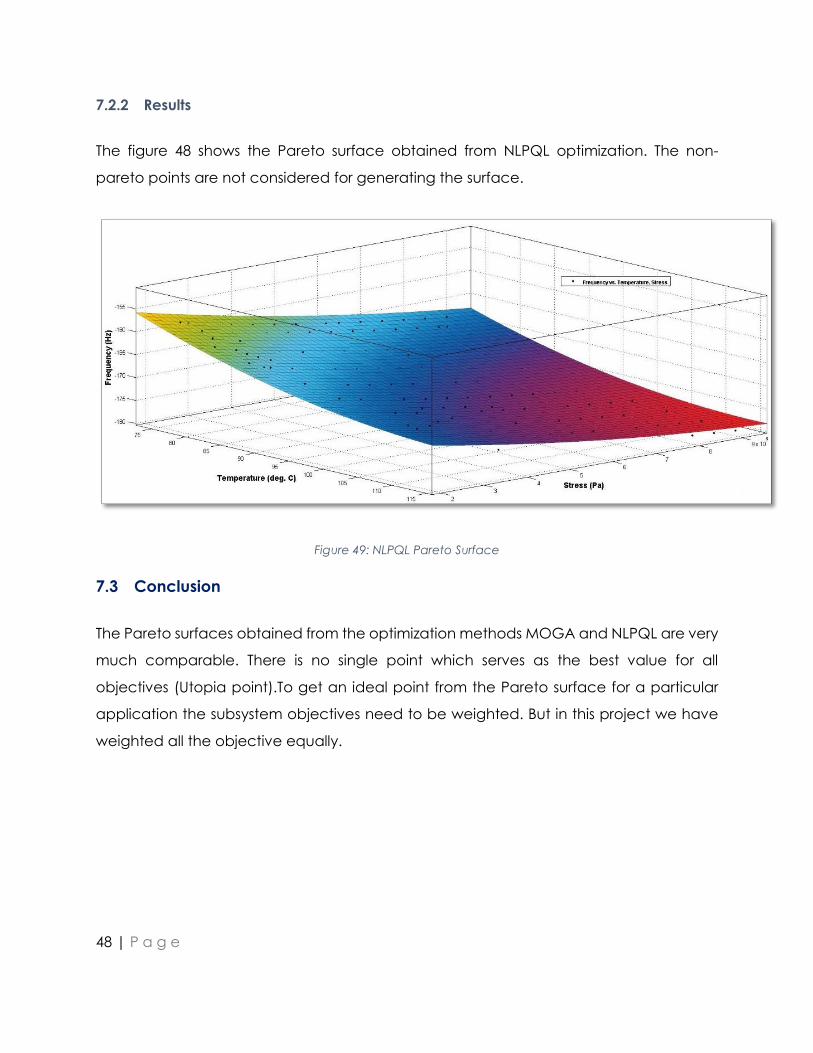
7.2.2 Results ..................................................................................................................... 48
7.3 Conclusion .................................................................................................................... 48
8 References ........................................................................................................................... 49
9 APPENDIX .............................................................................................................................. 50

6 | P a g e
Table of Figures
Figure 1: Clutch Assembly ........................................................................................................... 9
Figure 2: Schematic Diagram of subsystem optimization in ANSYS 15.0 ............................ 14
Figure 3: Subsystem Optimization Methodology .................................................................... 15
Figure 4: Parametric CAD model ............................................................................................. 17
Figure 5: ANSYS FEM model ....................................................................................................... 17
Figure 6: Boundary conditions, fixed support ......................................................................... 18
Figure 7: Rotational Velocity in Z direction .............................................................................. 19
Figure 8: Clamping pressure load applied on the friction lining .......................................... 20
Figure 9: Clutch lining constrained to rotate in Z direction only .......................................... 20
Figure 10: Constraints applied on flywheel ............................................................................. 21
Figure 11: Heat flux applied on the friction pads ................................................................... 22
Figure 12: Loads applied for heat dissispation ....................................................................... 22
Figure 13: Frequency vs Lining Face Thickness ....................................................................... 24
Figure 14: Frequency vs Lining Thickness ................................................................................. 25
Figure 15: Frequency vs Lining Inner Diameter ....................................................................... 25
Figure 16: Equivalent Stress vs lining face thickness ............................................................... 26
Figure 17: Equivalent Stress vs Lining Inner Diameter ............................................................. 26
7 | P a g e
Figure 18: Equivalent Stress vs Lining Thickness ....................................................................... 27
Figure 19: Temperature vs Lining Inner Diameter ................................................................... 27
Figure 20: Temperature vs Lining Thickness ............................................................................. 28
Figure 21: Temperature vs Lining Thickness ............................................................................. 28
Figure 22: 668.67 Hz .................................................................................................................... 30
Figure 23: 253.96 Hz .................................................................................................................... 30
Figure 24: 167.44 Hz .................................................................................................................... 30
Figure 25: 167.42 Hz .................................................................................................................... 30
Figure 26: DOE samples ............................................................................................................. 31
Figure 27: Optimized Design ..................................................................................................... 32
Figure 28: Goodness of fit .......................................................................................................... 33
Figure 29: Influence of parameters on output ....................................................................... 33
Figure 30: Local Sensitivity Chart .............................................................................................. 34
Figure 31: Convergence Criteria .............................................................................................. 35
Figure 32: Temperature distribution at the end of slip time .................................................. 35
Figure 33: DOE samples ............................................................................................................. 36
Figure 34: Optimized Final Design ............................................................................................ 37
Figure 35: Optimized Input values ............................................................................................ 37

8 | P a g e
Figure 36: Goodness of fit .......................................................................................................... 38
Figure 37: Influence of Parameter values ............................................................................... 38
Figure 38: Sensitivity Chart ......................................................................................................... 39
Figure 39: Covergence Criteria ................................................................................................ 39
Figure 40: Stress values at the end of slipping period ............................................................ 40
Figure 41: DOE Samples ............................................................................................................. 41
Figure 42: Optimized Design ..................................................................................................... 41
Figure 43: Goodness of Fit ......................................................................................................... 42
Figure 44: Influence of Parameter values ............................................................................... 43
Figure 45: Sensitivity Chart ......................................................................................................... 43
Figure 46: Convergence Criteria .............................................................................................. 44
Figure 47: System Optimization schematic diagram ............................................................. 45
Figure 48: MOGA Pareto Surface ............................................................................................. 46
Figure 49: NLPQL Pareto Surface .............................................................................................. 48

9 | P a g e
1 Design Problem Statement
The primary aim of this work is to design a rigid drive clutch system that meets multiple
objectives such as Vibrational rigidity, Structural and Thermal strength. Also, to
demonstrate a systematic approach to solving multi-objective problems by Response
Surface Optimization to obtain Pareto optimal solutions.
Figure 1: Clutch Assembly
Gradual engagement clutches like the friction clutches are widely used in automotive
application for the transmission of torque from the flywheel to the transmission. The three
major components of a clutch system are the clutch disc, the flywheel and the pressure
plate. Flywheel is directly connected to the engine's crankshaft and hence rotates at the
engine rpm. Bolted to the clutch flywheel is the second major component: the clutch
pressure plate. The spring-loaded pressure plate has two jobs: to hold the clutch assembly
together and to release tension that allows the assembly to rotate freely. Between the
flywheel and the pressure plate is the clutch disc. The clutch disc has friction surfaces
similar to a brake pad on both sides that make or break contact with the metal flywheel
and pressure plate surfaces, allowing for smooth engagement and disengagement.
When the clutch begins to engage, the contact pressure between the contact surfaces
will increase to a maximum value at the end of the slipping period and will continue to
stay steady during the full engagement period. During the slipping period, large amount

10 | P a g e
of heat energy is generated at the contact surfaces, which gets converted to thermal
energy by first law of thermodynamics. The heat generated is dissipated by conduction
between the clutch components and convection to the environment. Another loading
condition is the pressure contact between the contact surfaces that occurs due to the
axial force applied the diaphragm spring. In addition to the above output responses, this
work also considers the Vibrational characteristics of the clutch plate during the full
engagement period. The engine and the transmission components experience
dynamically varying loads during normal operation. This will cause vibrations and hence,
one must design the clutch system so as to avoid resonance with the transmission and
engine components.
2 General Nomenclature
P1 – Friction pad inner diameter
P2 – Friction pad thickness
P3 – Friction facing thickness
Ri – Inner radius of clutch disc in meters
Ro – Outer radius of the clutch disc in meters
N – Speed of engine in rpm = 3750 rpm
ωr – angular velocity in rad/s
Pmax – clamping pressure in MPa
3 Mathematical Calculations
The material considered for the friction pad is Kevlar 49 Aramid. Uniform Wear Theory is
considered for calculations, and accordingly, the intensity of the pressure is inversely
proportional to the radius of friction plate.

11 | P a g e
𝑅 =𝑅𝑖 + 𝑅𝑜
2= 0.1𝑚
In general, the frictional torque acting on the clutch plate is given by
𝑇 = 𝑁 × μ × W × R
In general, the frictional torque acting on the clutch plate is given by 𝑊 = 3000𝑁
𝑃 × 𝑟 = 𝐶 (𝑐𝑜𝑛𝑠𝑡𝑎𝑛𝑡)
Axial force on the clutch pad,
𝑊 = 2𝜋 × 𝐶 × (𝑅𝑜 − 𝑅𝑖)
𝐶 = 0.0119𝑁𝑚
The maximum pressure occurs at the inner radius and the minimum pressure at the outer
radius.
In general, the frictional torque acting on the clutch plate is given by
𝑃𝑚𝑖𝑛 =𝐶
𝑅𝑜= 0.0994 𝑀𝑝𝑎
𝑃𝑚𝑎𝑥 =𝐶
𝑅𝑖= 0.1492 𝑀𝑝𝑎
Here, we consider the maximum pressure value obtained in the Finite Element Analysis of
the clutch plate.
4 Thermal Analysis
4.1 Nomenclature
T – Temperature of the disc in Celsius

12 | P a g e
Tl – Limiting temperature of the material in Celsius = 150ºC
µ - Coefficient of friction of the material = 0.4
k – Thermal conductivity of the material in Watts per meter Kelvin
h – Heat transfer coefficient of the material.in Watts per sq. meters per Kelvin.
q – Heat energy generated in watts
qf – heat flux in W/m2
t – Slip time in seconds = 0.5s
A – Area of a friction pad = 0.000931m2
4.2 Mathematical Calculations
𝜔𝑟 =2 × 𝜋 × 𝑁
60= 392.6 𝑟𝑎𝑑/𝑠
𝑞 = 𝜇 × 𝑃𝑚𝑎𝑥 × 𝜔𝑟 = 23.4375 𝑊
𝑞𝑓 =𝑞
𝐴= 25155 𝑊/𝑚2
5 Modal Analysis
5.1 Nomenclature
𝐹𝑒 – Engine frequency
𝑛 – Order of frequency (1st order & 2nd order)
𝑁𝑒 – Engine rpm range (1000 rpm-4750 rpm)
13 | P a g e
5.2 Mathematical Calculations
𝐹𝑒 =𝑁𝑒
60× 𝑛
6 Model Analysis and Sub- System optimization Study
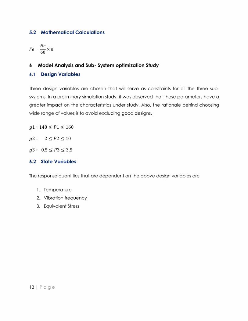
6.1 Design Variables
Three design variables are chosen that will serve as constraints for all the three sub-
systems. In a preliminary simulation study, it was observed that these parameters have a
greater impact on the characteristics under study. Also, the rationale behind choosing
wide range of values is to avoid excluding good designs.
𝑔1 ∶ 140 ≤ 𝑃1 ≤ 160
𝑔2 ∶ 2 ≤ 𝑃2 ≤ 10
𝑔3 ∶ 0.5 ≤ 𝑃3 ≤ 3.5
6.2 State Variables
The response quantities that are dependent on the above design variables are
1. Temperature
2. Vibration frequency
3. Equivalent Stress
14 | P a g e
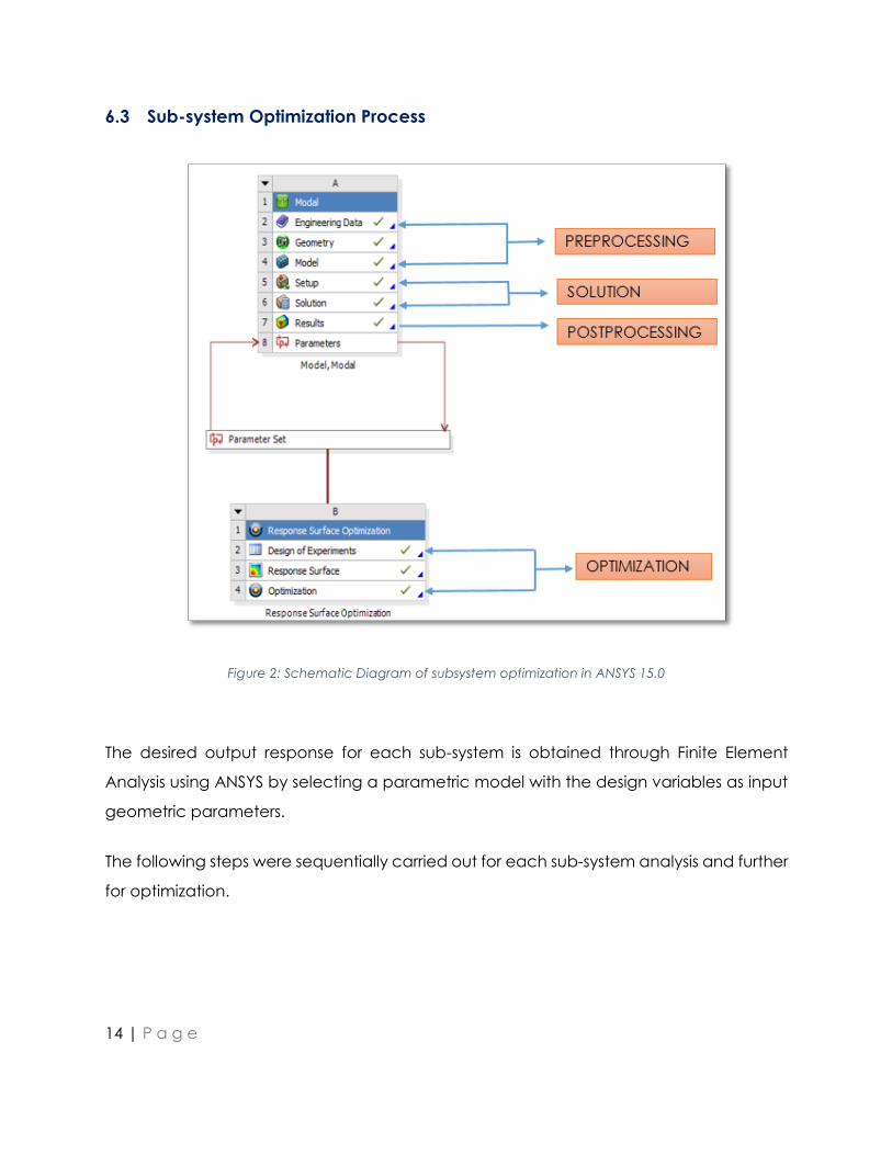
6.3 Sub-system Optimization Process
Figure 2: Schematic Diagram of subsystem optimization in ANSYS 15.0
The desired output response for each sub-system is obtained through Finite Element
Analysis using ANSYS by selecting a parametric model with the design variables as input
geometric parameters.
The following steps were sequentially carried out for each sub-system analysis and further
for optimization.
15 | P a g e
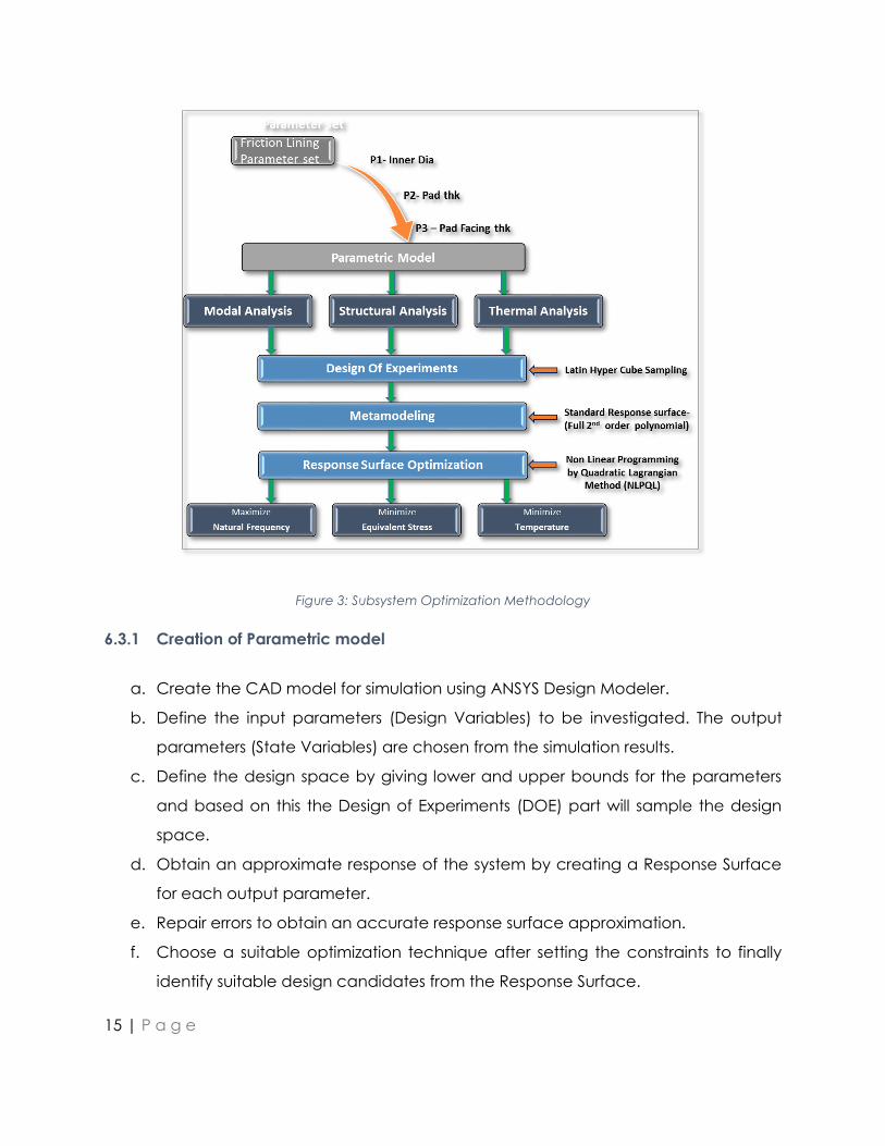
Figure 3: Subsystem Optimization Methodology
6.3.1 Creation of Parametric model
a. Create the CAD model for simulation using ANSYS Design Modeler.
b. Define the input parameters (Design Variables) to be investigated. The output
parameters (State Variables) are chosen from the simulation results.
c. Define the design space by giving lower and upper bounds for the parameters
and based on this the Design of Experiments (DOE) part will sample the design
space.
d. Obtain an approximate response of the system by creating a Response Surface
for each output parameter.
e. Repair errors to obtain an accurate response surface approximation.
f. Choose a suitable optimization technique after setting the constraints to finally
identify suitable design candidates from the Response Surface.

16 | P a g e
6.4 Engineering Data
Engineering data involves defining clutch material and properties
Type Clutch base plate Clutch plate lining
Material Structural Steel Kevlar Aramide Fiber 49
Properties
Density 7850 1440
Young’s Modulus 2 × 10¹¹ Pa 1.12 × 10¹¹ Pa
Poisson’s Ratio 0.3 0.36
Bulk Modulus 1.667 × 10¹¹ Pa 1.333 × 10¹¹ Pa
Shear Modulus 7.6923 × 10¹⁰ Pa 4.1176 × 10¹⁰ Pa
Specific heat Capacity 434 J kg^-1 C^-1 1420 J kg^-1 C^-1
Isotropic Thermal
Conductivity
60.5 W m^-1 C^-1 0.04 W m^-1 C^-1
Table 1: Kevlar Aramid Fiber 49 properties
6.5 Geometry
The base dimensions for the model are
Parameter Value
P1 160 mm
P2 2.7 mm
P3 0.8 mm
Table 2: Initial Input parameter values

17 | P a g e
Figure 4: Parametric CAD model
6.6 FEM model
Meshing is an integral part of the FEA process. The mesh influences the accuracy,
convergence and speed of the solution. A free mesh is applied with fine element size for
the CAD model. A free mesh has no specific element shape or pattern associated with
it.
Figure 5: ANSYS FEM model

18 | P a g e
6.7 Objective functions
6.7.1 Modal Analysis
Maximize the 1st order frequency to avoid resonance with Engine and Transmission
vibrations.
6.7.1.1 Boundary conditions & Loads
Since this is free vibration analysis, no external forces or loads were applied onto the FEM
model. Practically, while measuring the clutch plate natural frequency, it is mounted on
its base plate hole .In ANSYS simulation, the clutch plate given was fixed support
constraint at its base plate hole diameter.
Figure 6: Boundary conditions, fixed support

19 | P a g e
6.7.2 Structural Analysis
Minimize the Max. Equivalent stress acting on the friction pad
6.7.2.1 Boundary conditions & loads
1) The relative rotational velocity between the clutch plate & flywheel for t = 0.5 s slip
is applied on the clutch plate. Here the clutch plate is made to rotate with flywheel
kept stationary.
Figure 7: Rotational Velocity in Z direction
2) The contact pressure on clutch plate exerted by the pressure plate is applied on
the clutch plate surface as per calculated value.

20 | P a g e
Figure 8: Clamping pressure load applied on the friction lining
3) The clutch plate is constrained to rotate only about Z direction.
Figure 9: Clutch lining constrained to rotate in Z direction only

21 | P a g e
4) The flywheel is given fixed support constraint and is constrained for no rotation in
all directions.
Figure 10: Constraints applied on flywheel
6.7.3 Thermal Analysis
Minimize the Max. Temperature due to the heat generated on friction pad
6.7.3.1 Boundary conditions & loads
1) During engagement of the clutches, the friction surface is in contact with the
flywheel. The maximum heat flux of 25155 W/m2 is applied onto the friction pads.
The initial temperature for the analysis is set at ambient temperature (35 degree
Celsius).

22 | P a g e
2) The heat generated by the clutch engagement is dissipated through convection
and radiation. A convective heat transfer coefficient of 40 W/m2 (of free air) is
applied. For radiation 35 degree Celsius was applied
Figure 12: Loads applied for heat dissipation
Figure 11: Heat flux applied on the friction pads

23 | P a g e
6.8 Design of Experiments
The next step is to establish a relationship between the design variables and the output
response. Since all the design variables are continuous within their bounds, one needs to
sample the design space to determine how many and which parameters should be
chosen for creating a response surface. Here, the widely used stochastic sampling
technique, Latin Hypercube Sampling (LHS) is adopted. A set of l samples are randomly
generated regardless of the number of design variables. The advantage of LHS is that the
samples do not share the same values on any variable and hence offers a good
distribution in the design space. Also, unlike other deterministic methods like Central
Composite Design (CCD) and Full factorial methods, the number of simulations required
for LHS remain constant (after converging to a maximum) even with an increasing
number of parameters. At the end of this stage, output parameters corresponding to the
design points as defined by the DOE is obtained.
6.9 Metamodeling
Further, using metamodeling (regression analysis) techniques, a response surface that
provides a functional relationship between the output response and the input
parameters is generated. A full second order polynomial is the preferred model and uses
the method of least squares to determine the value of the unknown coefficients A, B and
C in the second order polynomial, Ax2 + Bx + C. The advantage of nonlinear least squares
regression like the second order polynomial over many other techniques is the broad
range of functions that can be fit.
6.10 Response Surface Optimization
Now that the meta-model of the problem has been developed, gradient-based
methods can be applied to search for the optimal point in the response surface. When
the design variables are continuous and the optimization is single objective, NLPQL (Non-
Linear Programming with Quadratic Lagrangian) is a very efficient algorithm. NLPQL uses
quasi-Newton methods to converge to the solution. It generates a sequence of QP sub-

24 | P a g e
problems which is obtained by quadratic approximation of the Lagrangian function and
linearization of constraints. And finally, to stabilize and ensure global convergence, an
Armijo line-search is performed.
Once the response surface optimization is completed, a manual refinement of the
response surface is done by inputting the optimal point as a design point and re-solving
the optimization problem until a good approximation of the actual response is obtained.
6.11 Parametric Study
The effect of input parameters on output parameter is studied from design sample space
and the variation of output parameter against each input parameter is plotted
6.11.1 Modal Analysis
Below graphs show the response in frequency with the change in input parameters.
Figure 13: Frequency vs Lining Face Thickness

25 | P a g e
Figure 14: Frequency vs Lining Thickness
Figure 15: Frequency vs Lining Inner Diameter
26 | P a g e
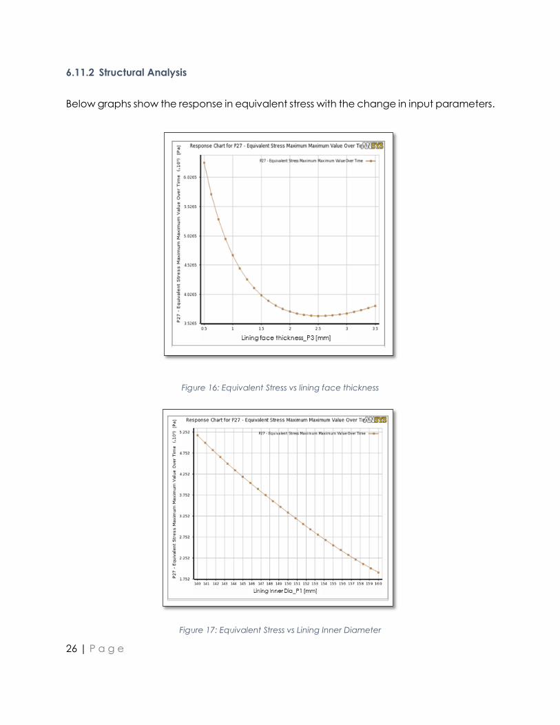
6.11.2 Structural Analysis
Below graphs show the response in equivalent stress with the change in input parameters.
Figure 16: Equivalent Stress vs lining face thickness
Figure 17: Equivalent Stress vs Lining Inner Diameter

27 | P a g e
Figure 18: Equivalent Stress vs Lining Thickness
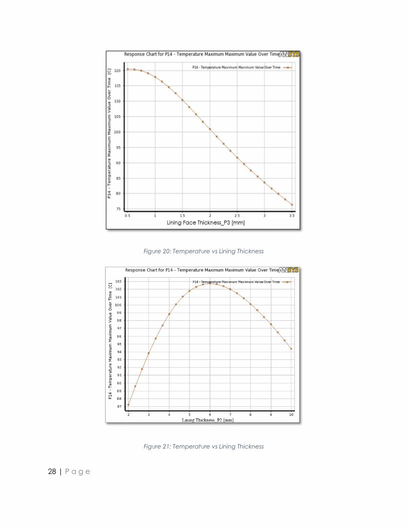
6.11.3 Thermal Analysis
Below graphs show the response in maximum temperature with the change in input
parameters.
Figure 19: Temperature vs Lining Inner Diameter
28 | P a g e
Figure 20: Temperature vs Lining Thickness
Figure 21: Temperature vs Lining Thickness

29 | P a g e
6.12 Discussion of Results
6.12.1 Modal Analysis (Vibrational Analysis)
The basic equation solved in a typical undamped modal analysis is the classical Eigen
value problem
[𝑲]∅𝑰 = 𝝎𝒊𝟐[𝑴]∅𝑰
Where
[𝑲] = Stiffness matrix
∅𝑰= Mode shape vector (Eigen vector) of mode
𝝎𝒊 = Eigen value
Ω =Natural circular frequency
By default, ANSYS Mechanical APDL uses Block Lanczos Mode Extraction Method to
extract modes
Following natural frequencies are reported after simulation
Mode Frequency[Hz]
1 167.42
2 167.44
3 253.96
4 668.67
Table 3: Frequency response

30 | P a g e
The mode shapes are
Figure 24: 167.44 Hz Figure 25: 167.42 Hz
Figure 22: 668.67 Hz Figure 23: 253.96 Hz
31 | P a g e
The engine rpm range is from 1000 rpm (idling speed) to 4750 rpm (engine fly-up
rpm).Taking into standard operating tolerance of 10% on the frequency range, the
corresponding 1st order frequency range is 18.326 Hz- 87.076 Hz and 2nd order frequency
ranges 36.663 Hz -174.163 Hz. These are the frequency bands with which clutch plate
frequency should be decoupled.
Here, the first mode frequency is considered as the output parameter for optimization as
it is the fundamental natural frequency. The 1st natural frequency (167.42 Hz) needs to be
optimized so that it doesn’t fall into the engine frequency band thereby avoid
resonance.
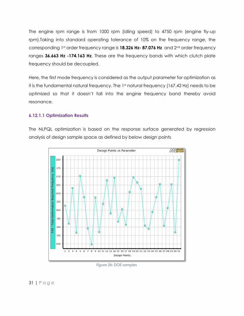
6.12.1.1 Optimization Results
The NLPQL optimization is based on the response surface generated by regression
analysis of design sample space as defined by below design points
Figure 26: DOE samples

32 | P a g e
With optimization, there is 7.42 % improvement in the output frequency which doesn’t fall
in engine frequency band.
Figure 27: Optimized Design
Parameter Starting Point Final Design
P1 (mm) 160 140 (active)
P2 (mm) 2.7 2 (active)
P3 (mm) 0.8 0.5 (active)
Output Initial Value Optimized Value Simulated Value
Frequency (Hz) 167.42 180.47 179.85
Table 4: Optimized Input Parameter Values
The above table shows the predicted value from NLPQL and observed value from ANSYS
Simulation are very close enough.

33 | P a g e
6.12.1.1.1 Robustness of Solution (Goodness of Fit)
Goodness of Fit shows that the output parameter has been very well approximated by
the response surface. The coefficient of determination is 0.99876.
Figure 28: Goodness of fit
Figure 29: Influence of parameters on output

34 | P a g e
From the above contour plots for output frequency vs Input Parameters, it can be seen
that the at the lower bound of all the constraints g1,g2 &g3,the function is monotonically
increasing and the constraints are active.
The output frequency can be maximized further if the lower bound of constraints are
relaxed.
Figure 30: Local Sensitivity Chart
Local Sensitivity Curve shows the impact of each input parameter on output.

35 | P a g e
Convergence Criteria shows the no. of Iterations required to achieve optimal solution
Figure 31: Convergence Criteria
6.12.2 Thermal Analysis
The change in maximum temperature with respect to time on application of the heat
flux and other loads is as shown below. The maximum temperature reached with the
initial design at the end of 0.5 seconds, the slip time, is 109.9 degree Celsius
Figure 32: Temperature distribution at the end of slip time

36 | P a g e
This output maximum temperature has to be minimized so as to avoid the failure of friction
pad material due to repeated clutch engagements lowering its cooling period
6.12.2.1.1 Optimization Results
The NLPQL optimization is based on the response surface generated by regression
analysis of design sample space as defined by below design points.
Figure 33: DOE samples
With optimization, there is 31.3 % improvement in the output frequency which doesn’t fall
in engine frequency band.

37 | P a g e
Figure 34: Optimized Final Design
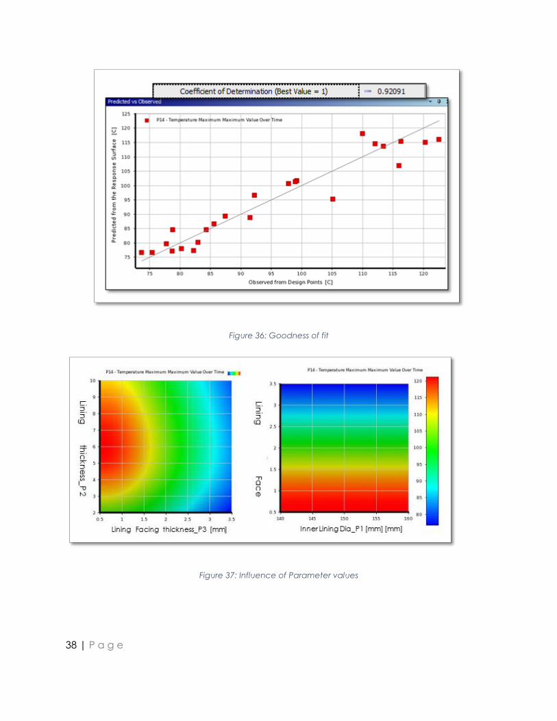
Robustness of Solution (Goodness of Fit)
Goodness of Fit shows that the output parameter has been very well approximated by
the response surface .The coefficient of Determination is 0.92091
Figure 35: Optimized Input values
38 | P a g e
Figure 36: Goodness of fit
Figure 37: Influence of Parameter values

39 | P a g e
From the above contour plots for Maximum temperature vs Input Parameters, it can be
seen that at the upper bound of the constraints g3, the function is monotonically
decreasing and the constraints is active from upper bound.
Local Sensitivity Curve shows the impact of each input parameter on output.
Figure 38: Sensitivity Chart
Convergence Criteria shows that two Iterations are required to achieve optimal
temperature.
Figure 39: Covergence Criteria
40 | P a g e
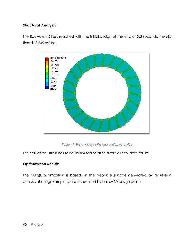
Structural Analysis
The Equivalent Stress reached with the initial design at the end of 0.5 seconds, the slip
time, is 2.5452e5 Pa.
Figure 40: Stress values at the end of slipping period
This equivalent stress has to be minimized so as to avoid clutch plate failure
Optimization Results
The NLPQL optimization is based on the response surface generated by regression
analysis of design sample space as defined by below 30 design points

41 | P a g e
Figure 41: DOE Samples
With optimization, there is 27.61 % improvement in the output frequency which doesn’t
fall in engine frequency band.
Figure 42: Optimized Design

42 | P a g e
The above table shows the predicted value from NLPQL and observed value from ANSYS
simulation are very close enough.
Robustness of Solution (Goodness of Fit)
Goodness of Fit shows that the output parameter has been very well approximated by
the response surface .The coefficient of Determination is 0.98149
Figure 43: Goodness of Fit
Parameter Starting Point Final Design
P1 (mm) 160 160(active)
P2 (mm) 2.7 10(active)
P3 (mm) 0.8 2.52
Output Initial Value Optimized Value Simulated Value
Stress(MPa) 0.254 0.18 0.185
Table 5: Optimized Input parameter values

43 | P a g e
Figure 44: Influence of Parameter values
From the above contour plots for Equivalent Stress vs Input Parameters, it can be seen
that at the upper bound of the constraints g1 & g2, the function is monotonically
decreasing and the constraints are active from upper bound.
Local Sensitivity Curve shows the impact of each input parameter on output
Figure 45: Sensitivity Chart
44 | P a g e
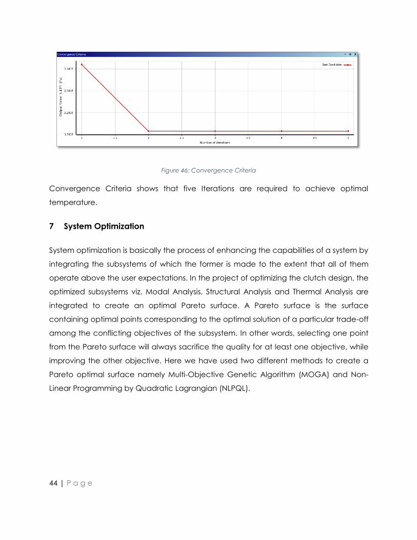
Figure 46: Convergence Criteria
Convergence Criteria shows that five Iterations are required to achieve optimal
temperature.
7 System Optimization
System optimization is basically the process of enhancing the capabilities of a system by
integrating the subsystems of which the former is made to the extent that all of them
operate above the user expectations. In the project of optimizing the clutch design, the
optimized subsystems viz. Modal Analysis, Structural Analysis and Thermal Analysis are
integrated to create an optimal Pareto surface. A Pareto surface is the surface
containing optimal points corresponding to the optimal solution of a particular trade-off
among the conflicting objectives of the subsystem. In other words, selecting one point
from the Pareto surface will always sacrifice the quality for at least one objective, while
improving the other objective. Here we have used two different methods to create a
Pareto optimal surface namely Multi-Objective Genetic Algorithm (MOGA) and Non-
Linear Programming by Quadratic Lagrangian (NLPQL).

45 | P a g e
7.1 Multi-Objective Genetic Algorithm (MOGA)
MOGA is a hybrid variant of the popular NSGA-II (Non-dominated Sorted Genetic
Algorithm). Only continuous problems can be solved using the same. The Algorithm goes
through several iterations retaining the elite percentage of samples through each
iteration and allowing the samples to evolve genetically until the best Pareto has been
found. As mentioned above this method can handle multiple goals. Some of the other
advantages are it helps identify the global and local minima of the function. It also
provides several candidates in different regions giving accurate solutions.
Figure 47: System Optimization schematic diagram

46 | P a g e
7.1.1 Optimization Process
The following steps were taken to generate the Pareto optimal surface using MOGA.
1. Three subsystems were integrated with the common input parameters as design
variables and the output as state variables.
2. Design of experiments was performed using Latin Hypercube Sampling (LHS)
3. A second order polynomial response surface was created from the DOE samples
generated.
4. Optimal solutions were generated from the response surface using MOGA
5. The deviation in the predicted value from the MOGA optimization and the
simulated value was corrected.
6. A Pareto optimal surface was generated using least squares regression analysis.
7.1.2 Results
The figure 47 shows the Pareto surface obtained from MOGA optimization. The non-
pareto points are not considered for generating the surface.
Figure 48: MOGA Pareto Surface
47 | P a g e
7.2 Non-Linear Programming by Quadratic Lagrangian (NLPQL)
NLPQL is a mathematical optimization Algorithm which solves non-linear programming
problems. In this method the objective function and the constraints are assumed to be
continuously differentiable. Here a sequence of QP sub problems are obtained by
quadratic approximation of the Lagrangian function. The problem size cannot exceed
2000 input variables and has to be well scaled. Though the method is fast, the accuracy
largely depends on the accuracy of the gradients. This is primarily used for single
objective problems but can also be used for multi-objective problems by constraining
the other output parameters.
7.2.1 Optimization Process
The following steps were taken to generate the Pareto optimal surface using NLPQL.
1. Three subsystems were integrated with the common input parameters as design
variables and the output as state variables.
2. Design of experiments was performed using Latin Hypercube Sampling (LHS)
3. A second order polynomial response surface was created from the DOE samples
generated.
4. Optimal solutions were generated by considering output frequency (maximize)
from the modal analysis as objective and constraining the other two output
parameters.
5. The deviation in the predicted value from the NLPQL optimization and the
simulated value was corrected.
6. A Pareto optimal surface was generated using least squares regression analysis.
48 | P a g e
7.2.2 Results
The figure 48 shows the Pareto surface obtained from NLPQL optimization. The non-
pareto points are not considered for generating the surface.
Figure 49: NLPQL Pareto Surface
7.3 Conclusion
The Pareto surfaces obtained from the optimization methods MOGA and NLPQL are very
much comparable. There is no single point which serves as the best value for all
objectives (Utopia point).To get an ideal point from the Pareto surface for a particular
application the subsystem objectives need to be weighted. But in this project we have
weighted all the objective equally.

49 | P a g e
8 References
1. http://mostreal.sk/html/guide_55/g-adv/GADV1.htm
2. http://inside.mines.edu/~apetrell/ENME442/Labs/1301_ENME442_lab5.pdf
3. Dr. Max Yi Ren, Notes for MAE 598: Design Optimization
4. How a car clutch works By Mike Bumbeck, automedia.com
5. http://www.dynardo.de/fileadmin/Material_Dynardo/dokumente/seminar/Doku
_Bearing_Angle_English_v12.pdf
6. http://www.hindawi.com/journals/isrn/2013/495918/
7. http://www.ansys.com/staticassets/ansys/conference/confidence/boston/down
loads/obtaining-and-optimizing-convergence.pdf
8. Design Optimization of the Rigid Drive Disc of Clutch Using Finite Element Method
9. Abdullah, O., Schlattmann, J., and Pireci, E., "Design Optimization of the Rigid Drive
Disc of Clutch Using Finite Element Method," SAE Technical Paper 2014-01-0800,
2014, doi:10.4271/2014-01-0800.
10. ANSYS. (2009). Design Exploration. Canonsburg: ANSYS.

50 | P a g e
9 APPENDIX
DOE SAMPLE SPACE FOR SUB SYSTEM OPTMIZATION
Modal Analysis

51 | P a g e
Structural Analysis

52 | P a g e
Thermal Analysis
53 | P a g e
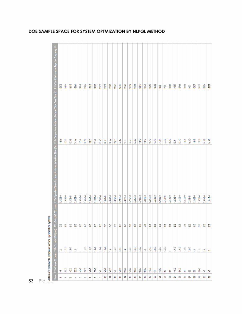
DOE SAMPLE SPACE FOR SYSTEM OPTMIZATION BY NLPQL METHOD

54 | P a g e
Frequency Table for NLPQL optimization
116.8597 111.86 106.86 101.86 96.86 91.86 86.86 81.86 76.86
865936.4 177.6863 177.3201 176.8206 176.0993 175.0604 173.6128 171.6858 168.8803 168.0506
815936.4 177.3113 162.5282 176.3479 175.5883 174.5206 173.055 171.122 168.6539 167.5011
765936.4 176.9213 176.4468 175.8511 175.0495 173.9501 172.4649 170.5253 168.0654 166.9204
464139.2 176.5141 175.9813 175.3301 174.4673 173.348 171.8411 169.8945 167.4437 166.3076
464139.2 162.5282 175.4977 162.5282 173.8869 172.714 171.1616 169.2119 166.7887 165.6624
464139.2 175.6316 174.9927 174.2208 173.2649 172.049 170.4919 168.5294 166.101 164.9859
562079.3 175.1461 173.3298 173.6337 172.5865 171.125 169.77 167.7984 165.3839 164.5663
507249.4 174.6223 173.8914 173.0161 171.9516 170.6417 169.0237 167.0424 164.6433 163.5544
456552.6 174.0514 171.8482 171.8482 171.2472 169.8971 168.2514 166.2609 163.8742 162.7962
415568.9 173.0372 172.0405 171.1161 170.4926 169.1067 167.4364 165.4369 163.0596 161.9905
362596.5 172.446 171.4846 170.8603 169.35 168.2512 162.8555 164.55 162.1796 161.1179
315936.4 171.9203 171.0267 169.9832 168.7561 167.45 165.592 162.0338 161.6101 160.7216
265936.4 170.3167 170.063 168.4536 167.718 166.2383 164.5031 162.4759 160.1134 159.0627
215936.6 162.8411 162.8411 162.8411 162.8411 162.8411 162.6585 160.9297 157.3006 155.21
211203.7 160.7008 160.7008 162.8411 160.7008 160.6785 160.5906 158.9318 155.1963 152.9876
stress
Temperature
Stress Table for NLPQL optimization
116.8597 111.86 106.86 101.86 96.86 91.86 86.86 81.86 76.86
116.8597 111.86 94.47533 101.86 96.86 91.86 86.86 81.86 76.86
116.8597 111.86 106.86 101.86 96.86 91.86 86.86 81.86 76.86
94.47533 111.86 106.86 101.86 96.86 91.86 86.86 81.86 76.86
94.47533 94.47533 106.86 94.47533 96.86 91.86 86.86 81.86 76.86
94.47533 111.86 106.86 101.86 96.86 91.86 86.86 81.86 76.86
100.4917 111.86 100.4917 101.86 96.86006 90.73919 86.86 81.86 76.86
100.0483 111.86 106.86 101.86 96.86 91.86 86.86 81.86 76.86
100.0535 111.86 100.0535 100.0535 96.86 91.86 86.86 81.86 76.86
113.9819 109.465 104.0225 100.098 96.86 91.86 86.86 81.86 76.86
113.4395 110.3675 105.1997 101.86 90.73919 91.86 86.12637 81.86 76.86
116.86 111.86 106.86 101.86 96.86 91.69632 86.86 79.54861 76.86
108.1493 108.1493 106.86 93.1717 96.86 91.86 86.86 81.86001 76.86
89.04096 89.04096 89.04096 89.04096 89.04096 89.0411 86.86 81.86 76.86
88.48115 88.48115 88.48115 89.04096 88.48115 90.33979 86.86 81.86 76.86

55 | P a g e
Temperature Table for NLPQL optimization
116.8597 111.86 106.86 101.86 96.86 91.86 86.86 81.86 76.86
116.8597 111.86 94.47533 101.86 96.86 91.86 86.86 81.86 76.86
116.8597 111.86 106.86 101.86 96.86 91.86 86.86 81.86 76.86
94.47533 111.86 106.86 101.86 96.86 91.86 86.86 81.86 76.86
94.47533 94.47533 106.86 94.47533 96.86 91.86 86.86 81.86 76.86
94.47533 111.86 106.86 101.86 96.86 91.86 86.86 81.86 76.86
100.4917 111.86 100.4917 101.86 96.86006 90.73919 86.86 81.86 76.86
100.0483 111.86 106.86 101.86 96.86 91.86 86.86 81.86 76.86
100.0535 111.86 100.0535 100.0535 96.86 91.86 86.86 81.86 76.86
113.9819 109.465 104.0225 100.098 96.86 91.86 86.86 81.86 76.86
113.4395 110.3675 105.1997 101.86 90.73919 91.86 86.12637 81.86 76.86
116.86 111.86 106.86 101.86 96.86 91.69632 86.86 79.54861 76.86
108.1493 108.1493 106.86 93.1717 96.86 91.86 86.86 81.86001 76.86
89.04096 89.04096 89.04096 89.04096 89.04096 89.0411 86.86 81.86 76.86
88.48115 88.48115 88.48115 89.04096 88.48115 90.33979 86.86 81.86 76.86
MATLAB CODE FOR REGRESSION ANALYSIS FOR MOGA
clc
clear all
A = xlsread('opti.xlsx');
Y = -A(:,3);
X1 = A(:,1);
X2 = A(:,2);
beta0 = ones(50,1);

56 | P a g e
X = [X1 X2 beta0 (X1.^2) (X2.^2) (X1.*X2)];
z = inv(X'*X);
b = z*X'*Y;
x1 = [0:0.01:1];
x2 = 0:0.01:1;
[X1,X2] = meshgrid(x1,x2);
for i = 1:length(x1)
for j = 1:length(x2)
y(i,j) =
b(1)*x1(i)+b(2)*x2(j)+b(3)+b(4)*x1(i)^2+b(5)*x2(j)^2+b(6)*x1(i)*x2(j);
end
end
surf(X1,X2,y);
xlabel('stress');ylabel('temp');zlabel('freq');

57 | P a g e
FREQUENCY-STRESS-TEMPERATURE TABLE (A) FOR REGRESSION ANALYSIS
Stress Temperature Frequency
895533.4214 83.18674111 168.5236306
652192.6985 85.93746706 167.6086429
621110.1679 86.13590557 165.5054552
685991.8803 90.96025367 170.5626591
673166.8557 87.61590634 166.2201614
657732.531 87.55078208 165.719328
302136.8415 81.21101819 157.8928123
438377.6904 81.70168443 158.0300236
289841.0455 81.89792073 158.0666637
737797.2284 94.11994465 171.4861478
481203.7145 86.65509461 162.8515439
473842.365 79.32038087 154.5857633
473085.4585 79.32038087 154.5607684
665677.9682 95.09799417 171.961458
417880.7784 87.90464731 163.1505045
457002.4378 78.53251736 152.712077
307965.2356 85.01967817 159.8649554
404709.3716 87.8755653 162.7579958
459408.5024 80.82121938 154.886515
421856.2728 79.32038087 152.8688587
473432.1719 83.93442786 157.3095171
548504.5337 94.86687358 168.8477205
401095.0935 88.88789379 161.5447877
297958.4156 80.58952886 151.5796391
429991.1465 78.77550798 149.4955515
429991.1465 78.77550798 149.4955515
336087.7617 88.88789379 159.8708133
264219.1465 87.94674043 157.1472155
425490.3686 81.78457336 149.9077393
209505.3171 80.58952886 148.5409389
418061.5303 99.43655218 169.3828325
418929.3845 99.6224907 169.447168
257164.8734 92.17404728 161.0075767
228545.6073 86.51849366 153.8341808
293182.9648 92.09552751 159.1107927
299530.6584 79.39109788 144.9571376

58 | P a g e


