ADAPTIVE SWTCHING CONTROL APPLIED TO MULTWARIABLE
SYSTEMS
Michael Chang
A thesis submitted in conformity with the requirernents for the degree of Doctor of Philosophy
Graduate Department of Electrical and Computer Engineering University of Toronto
@ Copyright by Michael Chang, 1997

National Library u*m of Canada Bibliothèque nationale du Canada
Acquisitions and Acquisitions et Bibliogrâphic Services services bibliographiques
395 Wellington Street 395. me Wellington OnawaON K 1 A O W Ottawa ON K1A ON4 canada Canada
The author has granted a non- L'auteur a accordé une licence non exclusive licence allowing the exclusive permettant à la National Library of Canada to Bibliothèque nationale du Canada de reproduce, loan, distnbute or sell reproduire, prêter, distribuer ou copies of this thesis in microform, vendre des copies de cette thèse sous paper or electronic formats. la forme de microfiche/& de
reproduction sur papier ou sur format électronique.
The author retains ownership of the L'auteur conserve la propriété du copyright in this thesis. Neither the droit d'auteur qui protège cette thèse. thesis nor substantial extracts firom it Ni la thèse ni des extraits substantiels may be printed or otherwise de celle-ci ne doivent être imprimés reproduced without the author's ou autrement reproduits sans son permission. autorisation.

In loving rnernory 01 rny father
and
tu our farnily

Therefore. the art of employing troops is that when the enemy occripies hi&
ground. do not confront him: with his back resting on hills. do not oppose him.
When he pretends to flee. do not piirsue. Do not attack his élite troops. Do
not gobbIe preferred baits. Do not thwart an enemy returning homewards. To
a surrounded enemy yoii must leave a way of escape. Do not press an enemy at
bay.

Adaptive Switching ControI Appiied to Muitivariable Systems
A thesis submitted in conformity wit h the requirements for the degree of Doctor of Philosophy
Graduate Depart ment of Electrical and Computer Engineering University of Toronto
@ Copyright by Michael Chang. i994
Abstract
In this thesis. a family of adaptive control problems is examined and solved using robust
self-tuning switching controllers. The motivation for using t his type of controller is t hat.
often in practise. no suitable mathematical mode1 of the system to be controled is available:
conventional methods of adaptive controller design generally require specific a priori plant
information (e.g. it may have to be known if the plant is minimum phase). and thus cannot
be implemented if such a knowledge is not known.
In contrast. this thesis shall generdy assume that very little a priori plant information is
known - the main assumption being that the plant çan be modelled by a finite dimensional
linear t ime invariant (LTI) system. More specifically. for the âdapt ive cont rol problem
of a family of not necessarily strictiy proper mult i-input mult i-output (XIIMO) plants.
a switching mechanisni which requires less a priori system information than previously
considered is proposed. Utilizing t his framework. vaxious new self-timing controlIers t hen are
presented. which solve the adaptive stabilization problem and the robust servomechanism
problem for potent iaIly unknown MIhI O systems.
The proposed controllers appear to be quite attractive in their overall improved tuning
transient response when compared wit h earlier results. Real- time experimentd results of one
part icular cIass of switching controllers when applied to a rnultivariable hydrauiic apparat us
are presented. and illustrate the feasibility of applying such adaptive controllers to industrial
process control problems.

1 would like to acknowledge the love. encouragement. and support t hat 1 have constantly
received from my parents. for without them. this current endeavoiu would not have been
possible. With the passing of my father. it is to him and our family that I dedicate this
work.
For academic. financial. and emotional support and guidance. many thanks go to my
supervisor. Professor Edward J. Davison. It has been an honour and a pleasiire to work
with him throughout my graduate years. and the knowledge and experiences thst 1 have
gained are imrneasurable.
Financial funding during my graduate stiidies also has been generously provided for by
the Satura1 Sciences and Engineering Research Council of Canada (YSERC) and the Uni-
versity of Toronto through XSERC Post Graduate Scholarships and University of Toronto
Open Fellowships respectively. For this. too, 1 am extremely grateful.
1 am also t hankful for the generous help in BT@2e provided by Christian Meder. and am
indebted to d l the members and s ta f f of the Systems Control Group for making my stay here
so fruitful and memorable. -1s well. my gratitude &O goes out to Mrs. Linda Espeut. our
Group Secretary. and hlrs. Sarah Cherian. our Graduate -Idmissions ancf Progrrtms Officer.
for their expert and thoughtful advice concerning the intricate and sometimes obfuscacory
rules and regdations of the University.
Last. but not least. 1 would iike to t hank al1 of my teachers - past. present. and future.

Contents
1 Introduction I
1.1 Notation 5' - . . . . . . . . . . . . . . . . . . . . . . . . . . . . . . . . . . . . . .
2 Adaptive Switching ControI of LTI MIMO Systems 8
. . . . . . . . . . . . . 2.1 Switching Control for Generd Controller Structures 8
. . . . . . . . . . . . . . . . . . 2.1.1 Preliminary Definitions and Results 9
. . . . . . . . . . . . . . . . . . . . . . . . . . . . . . . 2.1.2 Main Results 16
. . . . . . . . . . . . . . . . . . . . . . . . . . . . . . . . 2.2 SimulationResults 24
. . . . . . . . . . . . . . . . . . . . . 2.2.1 -1 Family of Three SIS0 Plants 24
. . . . . . . . . . . . . . . . . . . . . 2.2.2 A Family of Ten hlIMO Plants 28
. . . . . . . . . . . . . . . . . . . . . 7.2.3 X Fanlily of Five MIMO Plants 32
. . . . . . . . . . . . . . . . . . . 22.4 .A Family of UnstabIe SIS0 Plants 34
3 Adaptive Stabilization of LTI MIMO Systems 39
3.1 Adaptive Stabilization of First Order LTI SIS0 Systems . . . . . . . . . . . 39
. . . . . . . . . . . . . . . . . . . . . . . . . . . . . . . 3.1.1 bhinResults 43
. . . . . . . . . . . . . . . . . . . . . . . . . . . . 3.1.2 Simuiation Results -44
. . . . . . . . . . . . . . . . . 3.2 Adaptive S tabilization of LTI MIMO Systenis 44
. . . . . . . . . . . 3.2.1 Using a Known Value of the Compensator Order 50
. . . . . . . . . . 3.2.2 Using no Known Value of the Compensator Order 51
. . . . . . . . . . . . . . . . . . . . . . . . . . . . 3.2.3 Siniulation Results 53

4 The Self-Tuning Robust Servomechanism 65
. . . . . . . . . . . . . . . . . . . 4.1 Self-Tuning Proportional-Integral Control 65
. . . . . . . . . . . . . . . . . . . 4.1.1 Using an Estimate of the DC Gain 66
. . . . . . . . . . . . . . . . . . . 41.2 Using no Estimate of the DC Gain 71
. . . . . . . . . . . . . . . . . . . . . . . . . . . . 4.1.3 SimulationResults 72
. . . . . . . . . . . . . 1.2 Self-Tuning Proport ional-Integral-Derivat ive Control 75
. . . . . . . . . . . . . . . . . . . 4.2.1 Using an Estimate of the DC Gain 76
. . . . . . . . . . . . . . . . . . . 4.2.2 UsingnoEst imateof theDCGain 79
. . . . . . . . . . . . . . . . . . . . . . . . . . . . 4.2.3 SimulationResults 53
5 The Self-Tuning Servomechanism with Control Input Constraints 94
. . . . . . . . . . . . 5.1 Constrained Self-Tuning Proportional-Integral Control 94
. . . . . . . . . . . . . . . . . . . . . . . . . . . . . . . . 5.2 Simulation Results 101
6 Adaptive Tracking of LTI MIMO Systems 108
. . . . . . . . . . . . . . . . . . . . . . 6.1 Preliminary Definitions and Results LO8
. . . . . . . . . . . . . . . 6.2 Using a Known Value of the Compensator Order 112
. . . . . . . . . . . . . . 6.3 Using no Known Value of the Compensator Order 113
. . . . . . . . . . . . . . . . . . . . . . . . . . . . . . . . 6 . 4 Simulation Results 115
7 Experimental Results 125
. . . . . . . . . . . . . . . . . . . . . . . . . . . . . 7.1 Experimental Apparatus 125
. . . . . . . . . . . . . . . . . . . . . . . . . . 7.2 Linearized Model of MARTS 127
. . . . . . . . . . . . . . . . . . . . 7.3 Conventional Controller Design Results 131
. . . . . . . . . . . . . . . . . . . . . . 7.1 Switching Controller Output Results 194
. . . . . . . . . . . . . . . . . . . . . 7.4.1 Using a Known Estimate of 7 136
. . . . . . . . . . . . . . . . . . . . 7.4.2 Using no Known Estimate of 7 138
. . . . . . . . . . . . . . . . . . . . . . . . . . . 7 . 4 3 Using Controller C1 142
8 Conclusions 146
. . . . . . . . . . . . . . . . . . . . . . . . . . . . . . . 8.1 Summary of Results 146
. . . . . . . . . . . . . . . . . . . . . . . . . . . 8.2 Future Research Directions 147
vii
A Proofs of Main Results 151
A . 1 Adaptive Switching ControI of LTl MIMO Systenis . . . . . . . . . . . . . . 151
A . l . l Theorem2.1 . . . . . . . . . . . . . . . . . . . . . . . . . . . . . . . 151
A 2 Theorem 2.2 . . . . . . . . . . . . . . . . . . . . . . . . . . . . . . . 153
A.2 Adaptive Stabilization of LTI Systems . . . . . . . . . . . . . . . . . . . . . 161
2 Theorem3.1 . . . . . . . . . . . . . . . . . . . . . . . . . . . . . . . 161
A.2.1 Theorem3.2 . . . . . . . . . . . . . . . . . . . . . . . . . . . . . . . 162
A.3 The Self-Tuning Robust Servoniechanism . . . . . . . . . . . . . . . . . . . 165
3 . 1 Theorem4.2 . . . . . . . . . . . . . . . . . . . . . . . . . . . . . . . 165
A.3.2 Theorem4.4 . . . . . . . . . . . . . . . . . . . . . . . . . . . . . . . 167
A.3.3 Theorem 4.5 . . . . . . . . . . . . . . . . . . . . . . . . . . . . . . . 169
B Miscellaneous Data 171
B.1 Controller Parameters for a Family of Five Plants . . . . . . . . . . . . . . . 171
B.2 Partial Decentralized Control of a Multi-Zone Building . . . . . . . . . . . . 174
B.3 A Four Input-Four Output Furnace >Iode1 . . . . . . . . . . . . . . . . . . . 175
B.4 Matrices used for a Binary Distillation Tower . . . . . . . . . . . . . . . . . 180
C Additional Experimental Results
Bibliography
List of Figures
1.1 Simulated results of y ( t ) with (1.2) applied to (1.1). T
1 . . . . . . . . . . . . .
1.2 Simulatedresultswith(1.3)appliedto(1.1). . . . . . . . . . . . . . . . . . 7
2.1 .4 schematic setup of Controller F1 . . . . . . . . . . . . . . . . . . . . . . . 15
2.2 Simulated results with Controller FI applied to P3 when f (k ) = jl (k) . . . . 26
2.3 Simulated results with Controller FI applied to e3 when f (k) = f i ( k ) . . . . 26
2.4 Simulated results of P3 with supervisory controller [73] applied . . . . . . . . 27
2.5 New simulated results with Controller F 1 applied to Pi when f ( k ) = f (k) . 29
2.6 New simulated results with Controller F1 applied to P3 when f ( k ) = f2(k) . 29
2.7 Simulated results with Controller FI applied to Pio . . . . . . . . . . . . . . 32
2.8 New simulated results with Controller F1 applied to Pio . . . . . . . . . . . . 33
2.9 Switching tirne instants with ControIler F 1 applied to Plo . . . . . . . . . . . 33
2.10 Reference signals and switching time instants with ControlIer F1 appIied to
P, . . . . . . . . . . . . . . . . . . . . . . . . . . . . . . . . . . . . . . . . . . 35
2.11 Simulated response with Controller F1 applied to f i . . . . . . . . . . . . . . 35
2-13 (q = -0.5) Simulated response with Controller F1 applied to (2.9). . . . . . 37
3.13 (q = 0.125) SimuIated response with Controller F 1 applied to (2.9). . . . . . 35
2.14 (q = 0.5) Simulated response with Controller F1 applied to (2.9). . . . . . . 38
3.1 Simulatedresultsofy(t) withCoritrollerSIappliedto(3.1) . . . . . . . . . . 45
3.2 (w( t ) # O) Simulated results of y ( t ) with Controller S1 applied to (3.1). . . 45
3.3 Simulated results with Controller S2 applied to (3.5) using (3.6). . . . . . . 57
3.4 ( w ( t ) # 0) Simulated results with Controller S2 applied to (3.5) using (3.6). 57
3.5 Simulated results with Controller S2 applied to (3.5) usiug (3.7). . . . . . . 58
3.6 Simulated results with Controuer S2 applied to (3.8). . . . . . . . . . . . . . 60

. . . . . . 3.7 (.w ( t ) # O) Simulated results with Controller S2 applied to (3 .8) . 60
. . . . . . . . . 3.5 Simulated results witb Controller SS applied to Pi (s) (3.10). 62
. . . . . . . . . 3.9 Sirnulated results witli Controller 52 applied to P J s ) (3.10). 62
. . . . . . . . . 3.10 Simulated results with Controller S2 applied to Pj(s) (3.10). 63
. . . . . 3.11 Schematic set-up of the R, design synthesis used for P I ( . s ) (3.10). 63
. . . . . . 3.12 New simulated results with Controller S2 applied to Pi(.s) (3.10). 64
4.1 Simulated results with Controller P2 [14] applied to (4.5). . . . . . . . . . . 74
4.2 Simulated resiilts with Controller PI1 applied to (-4.5). . . . . . . . . . . . . 74
-4.3 Simulated results witti Controller 2 (641 applied to (4.5). . . . . . . . . . . . Y5
. . . . . . . . . . . 4.4 Simulated resiilts with Controller PID 1 applied to (4.5). 85
4.5 Simulated results with Controller PIDI' applied to (4.5). . . . . . . . . . . . Y7
. . . . . . . 4.6 ( p = O ) Simulated results with Controller PIDl applied to (4.5). 87
4.7 Simulated results with Controller PIDl applied to (4.11). . . . . . . . . . . 89
8 Simulated results with Lued integral cuntroller (4.13) ilpplied to (4.11). . . . 89
1.9 (DR # O ) Simulated resiilts w i th (filtered) Controller PIDl applicd to (4.14). 91
. . . . . . . . . . 4.10 Simulated results witti Controller PIDI applicd to (4.15). 93
4.11 ( ( p . E - ) = (0 . O ) ) Simulated resiilts with Controller PIDL applied to (4.15). . 93
5 . L Simulated resiilts with Coiitroller 2 [67] applied to (5.5). . . . . . . . . . . 105
5.3 Simulated results with Controller C l applied to (5.5). . . . . . . . . . . . . 103
5.3 Simulated results with Controller 2 [67] applied to a distillation tower . . . 106
5.4 Simulated results with Controller C l appliecf to a distillation tower . . . . . 106
5.5 Sirnulateci results with Controller 2 [W] applied tu (4.11). . . . . . . . . . . 107
5.6 Simulated results with Controller C l applied to (4.11). . . . . . . . . . . . 107
. . 6.1 Simulated results of y(t) with Controller T l applied to (6.6) iising (6.7). 116
6.2 Simulated results of y(t) with Controller T l applied to (6.8) using (6.9). . 118
6.3 Simulated results of y(t) with Controller T l applied to (6.10) using (6.12). 120
6.4 Simulated results of g ( t ) with Controller T l applied to (3.8) using (6.14). . 134
6.5 Simulated results of y ( t ) with Controller T l applied to (3.8) using (6.15). . 124
. . . 7.1 Schematic diagram of one possible MARTS arrangement (not to scale) 12G
7.2 Cross sectionai view of the intercounecteci columns of -MARTS (not to scale) . 128

. . . . . . . . . . . . . . 7.3 Experimental results with 0 = 30' and (7.5) applied
7.4 Experimental results with 0 = 30°? and with the outputs reversed at t = 1000
. . . . . . . . . . . . . . . . . . . . . . . . . . . . . . . . . . . . . . . seconds
7.5 Experimental results with t9 = 0°: and with the outputs reversed at t = 1000
. . . . . . . . . . . . . . . . . . . . . . . . . . . . . . . . . . . . . . . seconds
7.6 (N = 3) Experimental results with 0 = 40' and Controller PID 1 applied . . .
. . . 7.7 (N = 5) Experimental results with t9 = 40' and Controller PID 1 applied
. . . . . . . 7 Experimental results with 8 = 40" and Controller PID1' applied
7.9 (Reversed) Experimental results with 0 = 40' and Controller PIDl' applied .
. . . . . . . 7.10 Experimental results with 0 = 20' and Controller PIDI' applied
. . . . . . . . . . . . . . 7.11 Experimental results with Controller PID1' applied
. . . . . . . . . 7.12 Experimental results with 0 = 30" and Controller C1 applied
. . . . . . . 7.13 Experimental results with 0 = 30" and Controller 2 [67] applied
7.14 (Reversed) Experimental results with 6 = 30a and Controller C1 applied . .
7.15 (Reversed) Experimental results with 0 = 30" and Controller 2 [67] applied .
8.1 ( x ( 0 ) = 1) Simulated results with Controller 52 applied to (8.1). . . . . . .
8.2 (x(0) = 0.001) Simulated results with Controller S2 applied to (8.1). . . . .
. . . . . . . . . . . . . . C.1 Experimental results with Controller PID1' applied
. . . . . . . . . . . . . . C.2 Experimental results with Controller PID 1' applied
. . . . . . . . . . . . . . C.3 Experimental results with Controller PID 1' applied
. . . . . . . . . . . . . . C.4 Experimental results with Controller PID 1' applied
. . . . . . . . . . . . . . C.5 Experimental results with Controller PID 1' applied
. . . . . . . . . . . . . . C.6 Experimental results with Controller PID 1' applied
. . . . . . . . C.7 (Reversed) Experimental results with Controller PID1' applied
. . . . . . . . C.8 (Reversed) Experimental results with Controller PID1' applied
C.9 (Reversed) Experimental results with Controller PIDI' applied . . . . . . . .
C.10 (Reversed) Experimental results with Controller PIDI' applied . . . .
. . . . . . . . . . . . . . C.11 Experimental results with Controller PID1' applied
C.12 Experimental results with Controller PID1' applied . . . . . . . . . . . . . .

List of Tables
. . . . . . 4.1 Summary of the cyclic switching behaviour used for Figure 4.5. 84
7.1 Summary of the major components of !vIXRTS . . . . . . . . . . . . . . . . . 127
C . 1 Summary of the parameters used for Figures C . 1-C . 12 . . . . . . . . . . . . . 153
xii

Chapter 1
Introduction
In the convent iond design of controllers for rnultivariable systems, t Iie general approach
often adopted is to find a suitabie nominal model for the plant, which is often a difficult task,
and then to design a controller based upon this nominal model. In this case, if the nominal
model captures suflicient dynamicd aspects of the plant, effective control of the system
may be possible to attain. However, if large unexpected structural changes subsequently
occur in tlie system, severe limitations iri practical performance will, in general, arise since
conventional control schemes irsually do not have the ability to coritrol systenis wliicli are
subject to unplanned extreme changes.
Currently, one met hod to deal effectively wit h the specific problem of parametric plant
uncertainty is adaptive control; typically, the controllers erriployed in such schcrries are non-
Iinear and tinie-varying, and consist of a compensator augmentcd with a tuning rneciiariisrn
whicli adjusts the conipensator gains to match a prespecified desired plant tnodel. Although
recent attempts to enhance the robustness propert ies [42], [G]; iriiprove tlie closed loop tun-
ing transient response [go], [81], [10]? weaken the restrictive sufficient a priori assuniptious
[69], [74], [70], (991, and eliminate [77] tiie unwanted "bursting" pheno~nena 131 have been
successful for this class of controllers, these results generally are limited in scope due to the
nature of the a priori assumptions still required.
During the past several years, however, switching control in both theory and practice
has been applied successfully to multivariable systems to accomplish a wide variety of tasks
[131, [1011, [W, (591, [61], [64], [62] , (651, (661, [72], (791, [12], (151, [SOI, [16], (191, [SI], (101,
[23], [17], (731, [97]; while many controllers of this type wliich use very little a prion' plant
information have ais0 traditionally enjoyed the extra benefit of being very robust to large
plant urcertainties, one particuiar disadvantage of some of these schemes conimonly has
been an unpleasant closed loop susceptibility to substantial output transient responses. A
brief review of some of the important contributions made in this area can be found in [57]
and [58].
In this thesis, the primary focus therefore will be on designing simple d u s t adaptive
switching control aigorithms which attempt to use as little a priori system information as
possible, and which attempt to provide a reasonable closed loop transient resporise. For
instance, by now allowing for the possibility of cyclic switching to occur in the adaptive
control problem for a finite family of MIMO plants considered by Miller and Davison [65],
decreased closed loop tuning transients and a prion' system assumptions, as well as reduced
switching controller complexity, usually can be attained. Similarly. by utilizing this frame-
work to solve the adaptive stabilization probleni and the robust servomec~ianisni problem
for possibly unknown MIMO systems, corresponding desired t ransierit iniprovenients for
these problems can also gerlerally be achieved by selectirig nori-pathological coritroller and
tuning parameters.
In order to determine the feasibiIity of appIying such controllers to an industrial systelri,
real-tirne appIication studies using one such class of cont rollers wit h almos t uo a prion' plant
information, when applied to an experimentd multivariable liydraulic systerri. are carried
out; these studies show the feasibility of using the obtained controllers in ari iridustrial-
type setting and, in addition, show that the controllers applied display desirable iiitegrity
feat ures.
Before beginning, however, the following preliminary inforniation will be required.
1.1 Notation
The following mat hemat ical notation will be used irr a fairly corisistent rrianrier t hroiighout
t his t hesis.
Let R, IR+, N and @ denote respectively the set of real, positive real, natural: and
complex numbers; Rn (Cn) will be the n-dimensional real (cornplex) vector space. IRmXrL
(Cmxn) the set of m x n real (complex) matrices, C- (C') the set of complex riumbers with
strictly negative (positive) real parts, and @O the set of complex nunibers lying strictiy o n
1.1. Notation 3
the imaginaq axis. For any x? y € N,
x mod y := L - floor (i) Y
where floor(*) rounds the expression * down to the nearest integer.
With x = [xi x2 . . . xnIT E Rn. denote its pnorm as
and its oo-norm as
For any arbitrary A E C n x n . let X ( A ) and eig(A) denote the eigendues of -4. Matriu
A f RnXn will be said to be stable if X(A) c @- and unstable otherwise.
For the geaerd case when A E Xmx ". -+Ir will denote its matrix transpose. rank(;l) its
rank, and. if A also lias full row rank. di = - A ~ ( A A ~ ) - ' its pseudo-inverse. In addition. the
corresponding induced norms of A will be denoted as l1 - -Ll lp with the x-norm calculated as
and the Froberiius norm given as
where aij denotes the (i' j ) element of A.
As a final point, let C" (W") denote the set of Rn-valued functions defined on Bi which
are infinitely differentiable. A function f : Rç u {O) -r Rn will be said to lie in L, (f E L,)
if
1.2. Some Motivation 4
exists.
1.2 Some Motivation
As mentioned earlier, during the past several years, there bas been a considerable amount
of interest and effort made towards developing controller design methods which require
as little a priori plant information as possible [54], (341, (641, [62] , [6517 [72]' [23]: [17].
The motivation for this interest s t e m £rom the fact that it is generally difficirlt and often
impossible to obtain an accurate model representation of an actual industrial plant. As
well, while conventional adaptive controllers currently have the ability to deal effectively
with the problem of pararnetric plant uncertainty? important a priori plant information still
is required; for example, in conventional model reference adaptive control for a single-input
single-output (SISO) system, the four classical assumptions typically made are t hat [68]
[82]:
(i) the plant is minimum phase;
(ii) an upper boiind on the plaiit order exists and is k~iown;
(iii) the relative degree is known; and
(iv) the sign of the Liigh frequency gain is kiiown.
Altliough recent developnients have been able to reniove condition (iv) (691. [74], aiid to
weaken conditions (ii) [70] and (iii) [71], [98], given above, specific plant inforrnatiorl (e-g.
any plant zeros which lie in the open right half plane must be known to lie i r i a finite set
[63]) still is needed. For an excellent historical overview of some of the major advancements
in this area, see [75] and [76].
In this thesis, the primary focus will be on siniple prerouted adaptive switching control
algorithmsl whicli attempt to use as little a priori system information as possible; as well,
due to potent ial impleuientation constraints, t his work will also bc concerned with ro bust
- -. . . - - - -. - -- -
'A switching algorithm is said to bc prerouted if the potcntid sequence of applied controllers is dctermined off-line, and fixed prior to the application of the switching mechanism.
1.2. Some Motivation 5
adaptive schemes (cf. [go], for exampleo and the results contained t herein) which are tolerant
to bounded immeasurable noise disturbances? and which attempt to provide a reasonable
closed loop t ransient response.
As an illustration of the type of improvernent that may be obtained by using the proposed
controllers, consider the problem in [85] of finding a stabilizing controller (in the sense that
z ( t ) + O as t + cc and [x E L,' where ~ ( t ) and ~ ( t ) are? respectively. the state of the
plant and controller) of the form
for the one-dimensional SIS0 plant
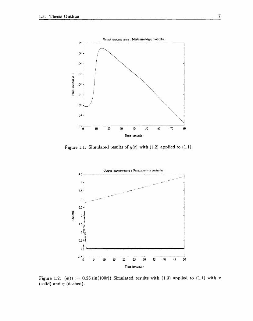
with botb b # O and a > O unknown. In ttiis instance. iising the blktensson-type [54]
cont roller (341
i ( t ) = $(t). ( 12a)
h(il) = d G . (1.2b)
and u(t) = y(t) - h(q(t))0-25 - (sin(JT;i;;iljT) + 1) -cos(h(q(t))) ( 1 .k)
with a := 1? b := -1, x ( 0 ) := 1: and q(0) := 1, the undesirably large transient response (with
a peak overshoot p a t e r than 31 1000 iri magnitude) presented in Figure 1.1 is obtained.
Similarly, using the adaptive Nussbaum-type stabilizer [85], [74? pg. 5491
with
1.3. Thesis Outline 6
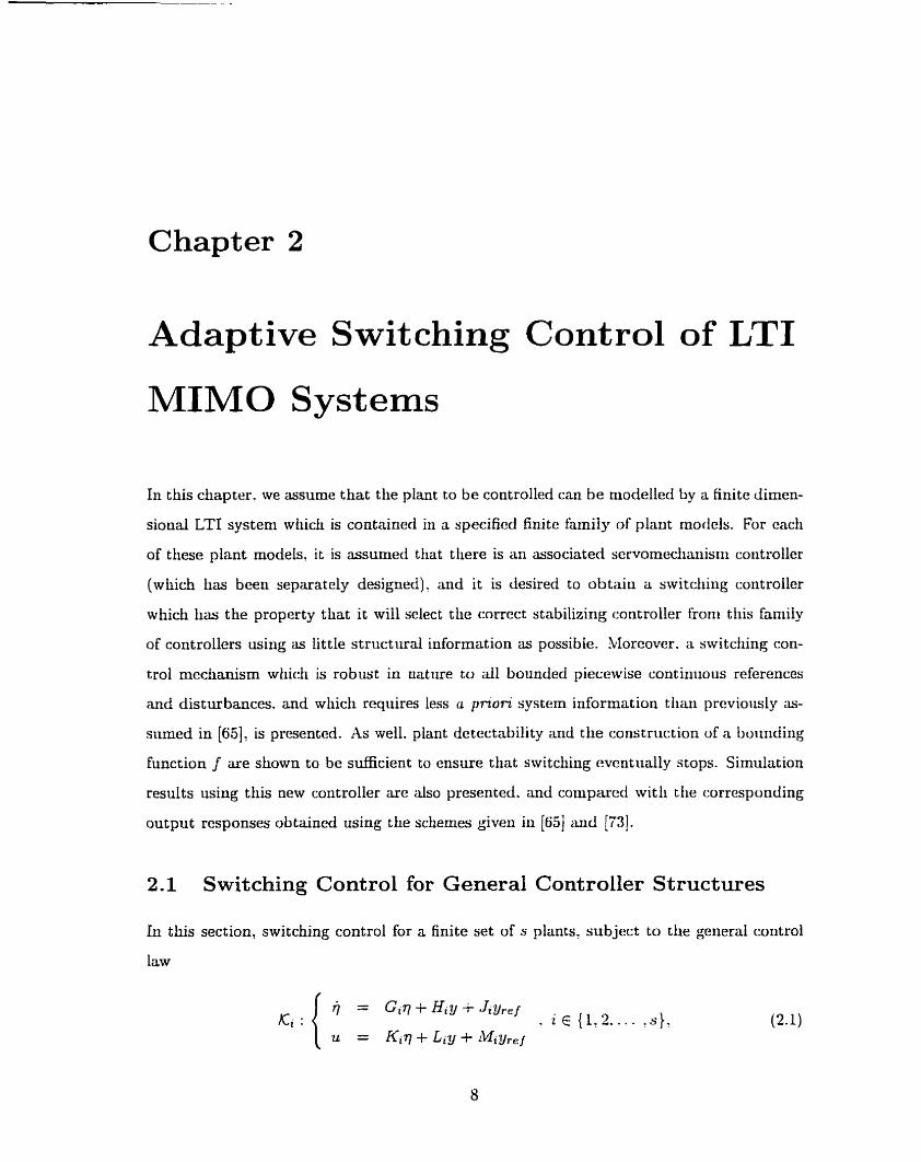
one can see t hat an arbitrarily small persistent measurernent dist urbance rnay destabilize
the system if ?12(t) is nonintegrable due to variations in e ( t ) . This effect can be seen in
Figure 1.2? where the controller given by (1.3) is applied to (1.1) with a := 1: b := 1.
x ( 0 ) := 1, q(0) := 0, and ~ ( t ) := 0.25sin(100t).
In contrast, using one of the new controllers proposed later in this thesis (Controler SI),
the more desirable responses shown in Figures 3.1 and 3.2 are obtained. whicb correspond
to the respective identical examples given for Figures 1. L and 1.2.
1.3 Thesis Outline
The remainder of this thesis is organized as fdlows.
In Chapter 2, the adaptive coritrol problem for a finite fanlily of MIXI0 LTI plants is
considered from the point of view of either stabilization or servomechanism control. and
new t heoreticd results for a generalized class of switching controllers are obtained. Chapter
3 then re-examines the adaptive stabilization problem for the case when the MIMO LTI
plant is almost entirely unknown (Le. it is assumed only that the plant is stabilizable and
detectable). In Chapter 4. the case of potentially unknown open loop stable 5IIMO plants
is considered. and self-tuning PI and PID controllers wliich solve the robust servoniech-
anism problem for constant reference and coustant dist urbauce inputs are proposed: the
corresponding PI case with control input constraints is next exaniined in Chapter 3. Tfiese
servomechanism controlIer results are generalized in Chapter 6 for the case of possibly un-
known MIMO plants. which may be open loop unstable. by applying an alternative niethod
for resolving the adaptive servomechanism problem. Real-time experimental results of one
class of coritrollers when applied to a multivariable hydraulic system then are preserited in
Ctiapter 7, showing the successful impleuientatiou of the PI and PID controllers developed
in Chapters 4 and 5.
1.3. Thesis Outline 7
Output response using a Mmensson-typc conmllrr. I
Figure 1.1: Simiilated results of y ( t ) with (1.2) applied to (1 .1 ) .
Output response usinor a Nussbriurn-rypt conuollrr. 4.5 r
. - - / - - - 1 - -
Figure 1.2: ( ~ ( t ) := 0.25 sin(100t)) Simulated results with (1.3) applied to (1.1) with s (solid) and q (daslied).
Chapter 2
Adaptive Switching Control of LTI
MIMO Systems
In this chapter. we assume that the plant to be controIled can be niodelled by a finite dimen-
sioiial LTI system which is contained in a specificd finite family of plant morlels. For each
of these plant rnodels. it is assumed that there is an associateci servomediariisin controller
(which has been separately designeci): and it is ciesired to obtain a switdiirig controller
which has the property that it will select the correct stabilizing controller froni ttiis faniiiy
of controllers using as little struct iiral information as possible. Moreover. a swi tdling con-
trol mechanism which is robust in nature to a11 boirnded piecewise contiriuoiis references
and disturbances, and whicb reqiiires less a prton' systern information t haxi prcvioiisly as-
siimed in [G], is presented. As well. plant detectability and the construction of a I~ouiiding
function f are shown to be sufficient to ensure that switching evcntrially stops. Simulation
results using this new controller are dso presented. and compareci witli the corresponding
output responses obtained using the schemes given in [65i and [73].
2.1 Switching Control for General Controller Structures
In this section, switching control for a finite set of s plants, subject to the general control
law
2.1. Switching Control For General Controller Structures 9
2.1.1 Preliminary Definit ions and Results
Let each element
belonging to the finite setL of possible plants to be controlled
be of the finite dimensional form
where x E IRn1 is the state. u IRm is the control input. g E Z r is the plant output to be
regulated, w E Rq is the disturbance, and e E Pr is the difference betweeri the specified
reference input g,,f and the output y. Ili tlie disciissious wtiicli will follow. we do not
necessarily assume that 7 ~ i , Ai: Bi? Cz, Di, Ei7 or Fi are known. and we do not restrict
X(Ai) C @-, i E {1,2,. . . , s ) .
Observe that upon applying Controller Ki to coritrol plant mode1 Pi ? the resiilting closed
loop system is
'since PI is a 6-tuple, a çlight abuse of notation is used to define P in an effort to maintain notational simplicity.

2.1. Switchine: Control for Generd Controller Structures 10
w here
fi := (1 - D,L~) - ' ( 2 . 3 ~ )
BiMi i B ~ L ~ Ï ~ D ~ M ~ Ei + B ~ L ~ Ï ~ F * and Bi := (2.3d)
Ji + Hi fi Di Mi H, Ïi F*
Preliminary definitions and results which are needed before proceeding are given as
folIows.
Definition 2.1: Consider matrices (C. A: B) E BrXn x Rn X n x RnXm. Then (C. A) is said
to be detectable if there exists a matrix K E Rnxr such that X(A + KC) C C-. and (A. B)
is said to be stabilizable if there exists a matrix L E Rmxn such that X ( A + B L ) C C-.
Definition 2.2 : (131. pg. 171) The transmission rems of (C. A. B. D ) E X r x n x RnXn x
Rn"" x WrXm are defined to be the set of complex numbers X which satis@ the following
inequali ty :
Definition 2.3: A plant Pi (2.2) is said to be m i n i m u m phase if al1 OF its transmission
zeros lie in @-; otherwise, phn t Pi is said to be non-minimum phase.
Definition 2.4: ( [ 2 6 ] ) Consider the triple (C. .4B) E ZarXn x Rn"" x Px ": t hen the set
of centralized féced modes of (C. A. B ) , denoted by A(C. -4, B) , is defined as follows:
Definition 2.5: ([24]) Consider (C, A, B' D) E WrX" x P nXn x W n X m x RrXm; then the
set of decentralized &ed modes of (C. A, B. D) with respect to K denoted by A(C. A B, D),
is defined as follows:

2.1. Switchin~: Control for General Controller Striictures 11
where K E IK is also chosen such that ( I - DK)-[ exists.
Remark 2.1: Given D E Rrxm: then for almost d l [30] L E B m X r . (1 - DL) E RrXr is
invertible (i.e. given a fixed matrk D. then ( I - DL) is invertible for generic L) . 0
Remark 2.2: Fkom Lemma 2.3.3 of 137: pg. 591, if 3 E gnXn and 11.T-11 < 1. tlien (1 - 3)
is nonsingular (Le. (1 - F)-l exists). 0
Definition 2.6: ([64]) A function f : N - 33- is said to be a s t m n g botrnding f irnction
(f E SBF) if it is strictly increasing and if
Definition 2.7: A function f : N + Ri is saki to be a modified strong bounding function
(f E MSBF) if it is strictly increasing and if? for al1 constants (cc) . ci , 0) 3- x Rt x Zt'.
Proposition 2.1: There exists a bISBF (e.g f ( 1 ) = i e x p ( i 2 ) ) .
Proof: The proof follows upon first observing that
for i > 2. In addition, since
i exp (i' ) i exp(i2) i- I 1
co + cl (i - 1) + c? cxp(i2) co + ci(i - 1) + c z C jexp(j2)

2.1. Switching Ccrntrol for General Controuer Structures 12
for (CO. ci. c 2 ) E P+ x !Ri x Wt: and since
the resuh immediately follows. D
Proposition 2.2: .Assume that -4, given in (2.3) is stable for a given cimice of (G,. Hi.
Ki, Li): then
X(Ai) êo for almost dI (Gi. Hi. Kt. L,).
Proof: The proof follows upon observing that -Xi can alternatively be written as
using Definition 2.4 and the fact that Ai is stable for a given choice of controllcr parameters
(G,. Hi. Kz. L,). it therefore foilows that -4, bas no fked modes lying in Co for al1 feedback
matrices
satidying the structure
where * is an arbitrary rnatrix having appropriate dimensions. Hence, it immediately follows
[30] that for alrnost ad controiler parasieters (Gia Hz: Ki. Li): X(Ai) CO. O

2.1. Switching Control for General Controller Structures 13
Remark 2.3: When Di = O for the proof of Proposition 2.2, one can alternatively express
Lemrna 2.1: Consider the system given in (2.2) with u( t ) given in (2.1) applied at t i z e
t = O. Assume that in (2.3): the matrk
is stable. and t hat yref(t) and w ( t ) are bounded piecewise cont inuous signais liaving respec-
tive L, norms of ljre and 6. Then there exist constants (Ci! CÏ' G' c-4) E P- x 22- x R' x R'
independent of z(0) = z0 := [ Z ( O ) ~ T ~ ( o ) ~ ] ~ such tiiat
for al1 t E [O,=).
Proof: Since Ai is stable, there exist coristants (A. C l ) E Bi x Rf sucli tliat / ~e - ' l ~ l l 5
for t 2 O; using the additional fact t hat
w here
t herefore

2.1. Switching Control for General Controller Structures 14
Likewise, since
it therefore follows that
w here
for al1 t E [O' co). (7
111 order to corisider the situation when gr, ( t ) and w ( t ) are boiinded coiit inuous signals.
and when Di = O for al1 i E ( 2 . 2 , . . . . s)' label Controller F1 as
t 1 := 0, and where, for each k 2 2 such that t k - # m, the switching tirne t k is defined by
1 i) t > t a - [ , and if this riiinimum exists

2.1. Switching Control for GeneraJ Controiier Structures 15
with f E MSBF. In addition, let Assumption F1 be the following:
i) Ilrl(0)ll < J(Ur
ii) l Ie(0) l~ < f (l)?
iii) for each plant Pi and each corresponding applied Controller K,, i E { 1.3. . . . . s ) ?
the closed loop system is stable (and controller parameters (G,, H i , .J,. K,. L,, -LIi)
provide acceptable error regulat ion/dis t urbance rejection when the plant Pi is subject
to bounded piecewise constant reference and disturbance inputs):
iv) for each plant Pi, (Ci, Ai) is detectable: and
v) for each i: j E {1.2.. . . .SI. (1 - DiLJ) is invertible (see Remark 2.1).
The switching mechanisrn described by Controller FI is schematically shown in Figure 2.1.
LU f
Plant
Figure 3.1: A schematic setup of Controller FI.
1'
Switch
In Controller F 1, norm bounds on q ( t ) and e ( t ) are used in an attempt
-
to detect closed
Cont roller
&
loop instability which might be caused if Controller Ki is applied to plant P,. i # j . If this
upper bound is met at a.ny time during the tuning process. then a controller switch occurs,
4
' ~ h i s condition is required so thac switching time tr, is well defined for Controller FI; given e ( 0 ) . it can be met easily by appropriatelx xaling f ( i ) .
2.1. Switchine Control for General Controller Structures 16
and is reset to zero irnmediately following this switch. This reset action is performed
since al1 candidate feedback controllers need not necessarily be of the same order, and
since past experimental investigations [14] have indicated that reduced tuning transient
responses generally can be attained via such a sclieme. However, for the case wtien al1
candidate controllers have the same order, i.e. when gi = gj for al1 i7 j E { 1: 2' . . . s } . rl(t:)
need not necessarily be reset to zero after each switch; one cari choose to continue to form
q( t ) iising the set of piecewise LTI systems given by (GiT Hi, J * ) witfi ~ ( t ; ) = q( t k ) .
2.1.2 Main Results
Continuous Signais
For the situation when Di = O for al1 i E {1'2,. . . .s), and wtieri yrel(t) and w ( t ) are
bounded continuous signals, the following result can be obtained:
Theorem 2.1: Corisider a plant P E P with Di = O, i E {1,2.. . . , s ) . and witli Coritroller
FI applied at tirne t = 0; tlien for every j E MSBF. for every bounded contiriiious reference
and disturbance signal, and for every initial condition z (0 ) := [ x ( o ) ~ v ( ~ ) T ] T for which
Assumption F1 holds, the closed loop systexxi has the properties tfiat:
i) t h e exist a finite tirne t,, 2 O and coristant matrices (Gss, H,,, J,,, Kss7 L,,, iCI,,)
such that (G( t ) , H ( t ) , J ( t ) , K ( t ) : L ( t ) h.l(t)) = (Gss, Hss: Jss: Kss, L,,, Alss) for al1 t >_
tss;
ii) the controller states q E Lm and the plant states x E L,; and
iii) if the reference and disturbance inputs are constant signais. tlien for alriiost al1 con-
trolier parameters (Gi, Hi, Ki Li), asymptotic error regulation occurs, i.e. e ( t ) + O as
t -+ XI.
Piecewise Continuous Signals
For the situation when Di # O for some i E { 1,2, . . . , s} and/or wlien yrel(t) or w(t) are
bounded piecewise continuous signals, the switching criterion given for t irne tr; in Controlier
F1 may not bc well-defined. ln order to circumvent such poteritiai problenis, Coritroller F1
2.1. Switching Control for General Controller Structures 17
can be simply modified by filtering the error signal r ( t ) , and defining e ( t ) as
Hence, label Assumption F2 and Controller F2 to be? respectively. Xssumption F1
with e ( t ) replaced by e ( t ) , and Controller F1 with e ( t ) replaced by ef ( t ) in the definition
of switching time t k .
Lemma 2.2: Consider the closed loop system fornied by augmenting (2.3) together with
(2.5). Assume that X(Ài) C @- and that y re f ( t ) and w(t ) are boiinded piecewise continuous
signals. Then there exist constants (Ci : C2) E W' x W+ independent of i ( 0 ) := [x(OIT r l ( ~ ) T
e such that
for al1 t E [ O , o o ) .
The following result can now be obtairied.
Theorem 2.2 : Consider a plant P E P with Controller F2 applied at time t = 0: then
for every f E MSBF and X E B+. for every bounded piecewise continuous reference and
disturbance signal, and for every initial condition Z(0) := [ Z ( O ) ~ ,"(O)= el (0)*IT for which
Assumption F2 liolds, the closed loop systeni lias the properties tliat:
i 1
ii)
iii)
there exist a finite time t,, > O and constant matrices (Cs, , H,,! Jss7 Kss? L,,. :LIss)
such that ( G ( t ) , H ( t ) : J ( t ) , K ( t ) , L ( t ) , h . l ( t ) ) = (Gss? Hss, Jss. K,,. L,,! 3.I,,) for al1 t 3
tss;
the controller states 17 E L,, the plant states x E Lm, and the filtercd error signal
e l E Ç,; and
if the reference and distubarice inputs are constant signals, theri for alniost al1 con-
troller parameters (Gi, Hi, Ki, Li), asyrnptotic error regulation occiirs, Le. e ( t ) + O as
t + 00.
Controller F2 provides a great deal of generality aud versatility sirice:

2.1. Switching Control for General Controller Structures 18
atl finite dimensional MII'vIO LTI plant models Pi are assunied to have the general
form given by (2.2), with Ai not necessarily stable, Di not necessarily equal to zero.
and Pi not necessarily minimum phase;
the plant models Pi need not be controllable and/or observabie:
rn the set of al1 admissible controllers need only satisfy the structure presented in (2. l) ,
and thus the candidate controllers need not have the same dimension;
rn the class of piecewise cont inuous reference and dis turbance sigrials allowable for the
servomechanism controller design [27] of Ki (and the irnplementation of Controller F2)
is quite large provided only that gr,/ E L, and w E Lm (e-g. the class of sinusoidal
references and disturbances is allowed);
a priori bounds on either y r e l ( t ) or w(t) are neither rieeded nor estiniated for the
proposed controller;
a rio extensive a pr ior i on-line calculations are iieeded in order to inipleme~it Controller
F2 (cf. the schenies given in [34] and [65]);
the controller switching meclianism is very simple to iniplement in real-time. and is
therefore attractive from a practical point of view;
the switching meclianism does not depend directly on any explicit knowledge of the
matrices associated with plant Pi or candidate Controller K,;
no on-line estimation period is needed; and
rn the switching mechanism is robust and will riot suffer frorri chattering in the stcady-
state (cf. [39], for instance) for al1 bounded piecewise continuous reference arid distur-
bance inputs.
As well, Theorems 2.1 and 2.2 will clearly d s o hold even if the finite number of candidate
controllers is greater than or equal to the nuniber of possible plants3.
In addition, in Theorem 2.2, tlie requirement that ( t ) and w(t) be bounded piecewise
continuous functions and the restriction that switching carmot occur infinitely fast guarau-
tees the existence and uriiqueness of a solution [41] to the set of differential equations given
3 ~ n fact, Theorems 2.1 and 2.2 will hold for an infinite number of plants (cg. see Section 2.2.4) so long as there exist a finite number of candidate controllers which satisfy Xssumptions F1 and F2 rcspectively.

2.1. Switchine: Control for General Controller Structures 19
by (2.3) and (2.5). Furthermore, without any loss of properties i) to iii) given in Theorem
2.2: filtered error signal e (t) couid also have been defined as
where II E EUr, X ( r l f ) C f -. and Cl and B are botli invertible.
In fact. for the general situation when plant P, is described by
properties i) and ii) of Theorem 3.2 will also hold for al1 boiinded pieccwise coritinuoiis
noise s ipals (pi: p) E R'i~~l x W z wi th ( N I - Q i ) E Rnt'<qbl x I P r " ' ~ ~ ~ . This follows since
the closed loop systeni with Controller K, applied rnay be expresseci as
w here
Moreover! if II[~: pr]Tll -t O, property iii) of Theoreni 2.2 will once again be recavered.
Since corresponding comments sirnilar to those given liere cari dso be made for Tlicorerns
2.1. S witchine; Control for General Controller Structures 20
3.1, 3.2, 3.3, 4.2, 4.3, 4.4, 4.5, 6.1, and 6.2 (provided that the output signals are filtered
accordingly) by using an identical argument, the details of these additional extensions will
be omit ted for brevity.
Remark 2.4: Let the switching time t k be defined as
if this minimum exists
I O 0 ot herwise,
and define Assumption A to be Assumption F1 with the following additional condition:
vi) H, is left invertible for al1 j E {l , 2, . . . , s ) (i.e. H j has full column rank. and hence,
there exists H: := (HTH~)-'HT such that HJH, = 1).
Then properties i) to iii) of Theorem 2.1 will also hold for al1 bounded piecewise coiitinuous
reference and disturbance signals with Dj not necessarily equal to zero for all j . This follows
since, for any plant Pm E P, the pair
is detectable. Furt herniore, under Assumpt ion A, if swit chhg based iipon filtered error
signal e (t) is still desired. then Theorem 2.2 will also hold for any (CI , Al B I ) E Wrf "f x
Wnf Xnf x Wnf x r with A(AI) c @-. 0
Remark 2.5: Define
where X E W'. Assume that
i) I I Y ~ ( O ) I I < f ( U a d
ii) lluj(0)ll < f (1)

2.1. Switching Control for Generd Controller Structures 21
both additionally hold. Then Theorem 2.2 wilf also hold using the switching criterion
defined by
i ) t > t k A l r and if this minimum exists t k :=
ii) I[S(t)lJ = f (Cc - I )
I ot herwise.
u- here
- ( t ) := [ T j ( q T yf(t)T]T.
Given the general nature of Controller F2. oue may aho want to bouud iridividually
~ ( t ) ruid e l ( t ) by differenr bounding functions. This can be done as showu in the following
definition and existence resul ts.
Definition 2.8: Functious f i : N -t Ri and f2 : N -t R- are said to be choosubie modified
stmng boundingfvnctions ((fi! f2) E CMSBF) if. for t E {l. 2}. fk is strictly increasing and
if, for al1 constants (CO, ci? C?. c3) E Ri x Ri x Ri x Wr.
Proposition 2.3 : There exist functions J 1 and f- such tbat (f [, f.?) E CMSBF (e.g.
ji ( 2 ) = cri exp(i2) and f2(i) = ,& exp(i2) where (a? 0) E xi x Et+).
2.1. Switching Control for Cenerai Controller Structures 22
Remark 2.6: Consider the switching criterion for Coritroller F2 given by
if this uiiuiniuni exists
where ( f i , f2) E ClviSBF. Then with
md witb conditions iii) to v) of A4ssiimption F3 assunled to be triie. Theoreni 2.2 will also
hold true in this situation. 0
Remark 2.7: The modifications given in Remaxk 2.6 can also be made to the switching
mechanisms given in Theorerus 3.2. 3.3. 4.2. 4.3. 4.4, 4.5. 6.1. and 6.2. 0
Remark 2.8: For simplicity, consider the case when Di = O. i f { 1.2. . . . . ..; ): tlien the ro-
bust servomechanism problem can be solved (if possible) iising the servocorr~peiisator design
method given in [27]. For example. maintaiiiing the structure. notation. aiid assiiniptioiis
given in [27]: with
e -- .- l/ - IJrej.
a full order Luenberger observer of the form
2 = (.Ai + C,Ci)i? + Biu - Ciy
c m be constructed to yield

2.1. Switching Control for General Controller Structures 23
where := 5 - z. Since the closed loop system rnay be expressed as
w here
IL = PO,i + Pt<.
one can therefore choose matrices Po, and Pi siich that
is stable. Hence. the final controller may now be expressed in the forni
One can tlierefore apply switdiing Controller F3 to repulate i~11d reject adaptivcly tiiis
particular class of bounded reference and disturbance signals. 0
Remark 2.9: For simulation purposes, with plant P liaving system matrices given by
(A, B. C. O, E. F ) ,
and with Controller Ki applied, the closed loop system may be expressed as
A Bpi B ~ o , [i l = [ -C;C B-G Biri C* Ai + CiCi O + BIPol ] [ j] + [;* -CtF U' ] [ J ï f ] 7

2.2. Simulation Results 24
where the same notation as given in Remark 2.8 is maintained.
2.2 Simulation Results
In this section, the output response obtained by applyiug Controller F1 to a faniily of
strictly proper plants will be considered. In the first example, results £rom the simulation
will be compared with other output responses formed using the schemes given in [65] and
[73]. For the second and third example. the iinstable batch reactor mode1 [23! will be used.
This section is concluded wit h results obtained by using the fmi ly of plants given in [31].
2.2.1 A Family of Three SISO Plants
Consider the following family of three SISO LTI plant models taken froni [65]:
Model Pl :
with open loop eigenvalues of -4.5 + 1.5j:
Model Pz:
witb open loop eigenvalues of 0.031 and -24.031; and
Model P3:

2.2. Simulation Results 25
wit h open Ioop eigenvalues of -3.535 and - 10.565. As one can v e r i k using
Controller KI : 7 j = e? u = -2.7577:
Controller ICz : 7 j = e. u = -2q + 79: and
Controller K3: 7j = e. u = 25q - ~ I J
conditions iii) and iv) of .4ssumption F1 are both satisfied. and al1 controller-plant mis-
matches result in a closed loop unstable system4.
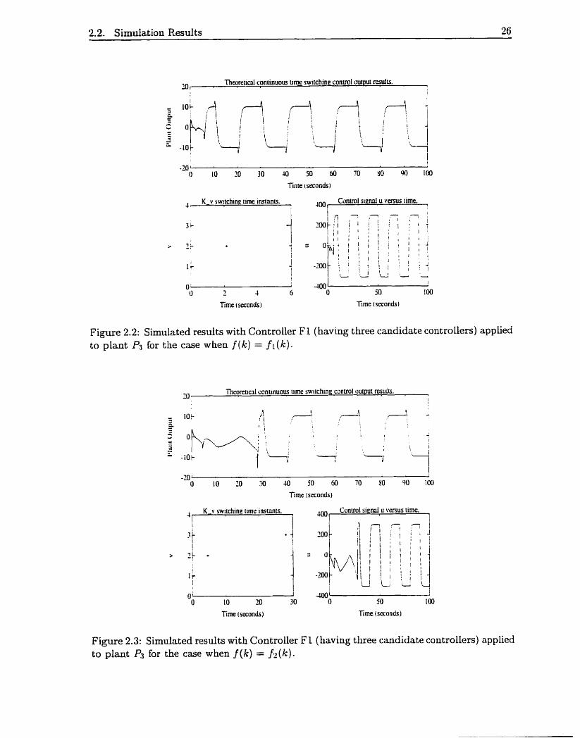
In Figures 2.2 and 2.3: the output response of the closed loop system with Controller F1
applied to plant P3 is given for the case when f (k) = f i (k) and j(k) = f2(k) respectiveiy.
w here
for each figure.
~ ( 0 ) := 0: w (t) := 2. and yref(t) is a square wave (beginning a t time t = O) having zero DC
offset, a peak magnitude of 10. and a period of 20 seconds. Furthermore. in both instances.
switches occur due to bounds on q ( t 2 ) and 71(t3) being met or exceeded.
As can be seen. in each case, the transient response rnight be considered to be quite
reasonable taking into account the fact t hat t here are t hree differeut poteut i d cont roller
candidates which m u t be considered. In coutrast, the transient peaks obtained using
Controllers 1 and 2 given in [65] are substantially larger for the same set of controller
candidates5. This occurrence is related in large part to the fact that Controller FI has a
potential cyclic switching action which may occur. whereas the switching rnechanisnis given
in [65] will, a t rnost, try each possible controller only once.
"-4 controller-plant mismatch is said to occur if Controller K, is applied to piant P,. where i f j . o or Controllers 1 and 2, the peak magnitude of the output trançients are approximately 2600 and 110
respec tively.
2.2. Simulation Results 26
Themtid sontinuous time switching conuol output rcsults. 1
, K v switchine rime instants. ,00 Conuul s i e d u venus fime.
,
0: O 1 4 6 O 50 100
Tirne I seconds Tirne isecondsl
Figure 2.2: Simulated results wit h Controller F 1 (having t hree candidate controllers) applied to plant P3 for the case when f (k) = fi(k).
Theoretical conirnuous rime swiichine control ciurpur mufis. IO - 1
-70' O 10 20 30 40 j0 60 70 Y0 90 100
Tirne (seconds)
, K v swrichine time instanu. Cantml s i e d u vcrsus time.
0; 1 1 O 10 10 30 O 50 100
Time (seconds 1 Time (seconds)
Figure 2.3: Simulated results with Controller F1 (having tliree candidate controllers) applied to p l a t l3 for the case when f (k) = f . - ( k ) .

2.2. Simulation Results 27
20 l Sirnulaed output response of P-3.
1
-IO il 10 10 j0 10 50 60 70 Y0 'H) 100
Time (seconds)
J r K v swiichtne tirne instmis.
- -
"0 0.05 0.1 0.15 0.2 0.3 0.3 0.35 0.4 0.45 0.5
Time iscconds)
Figure 2.4: Simulated results of plant Pi with supervisory controller [73] applied.
For further cornparison" Figure 2.4 shows the output response of plant Pi obtained
when using the SISO supervisory control switctiing mechanism given ixi [73]. Here. <Irurll
time rr, is set to be equal to 0.1 seconds. with
and Controiier K i is applied initictlly at time t = O. Simila to the simulations shown in
Figures 2.2 and 2.3,
w ( t ) := " M .
q ( 0 ) := o.
and ~ ( 0 ) := [1 21T.
Remark 2.10: The switching mechanisms for the controllers given in [65] and [73] gener-
ally necessitate more system information or a priori computation t han required for proposed
Controllers F1 and F2. For instance, explicit use of the family of SISO transfer functions
6 ~ h e author acknowledges the gracious help and assistance of Wen-CIiung Chang and A. S. Morse for providing the simulation code uscd to generate Fibwrc 2.4.
2.2. Simulation Resdts 28
is needed in [73], while knowledge of each candidate
(A. B. C. O. E. F )
system matrix is requùed in [65]. As such. it is conjectured that the switching mechanisms
given by Controllers F1 and F2 will be more robust with respect to unmodelled plant
perturbations and immeasurable noise disturbances than those mechanisms given in [65]
and [73]. O
Remark 2.11 : In Figure 2.4? dwell time rg c m be chosen to be 0.1 seconds since r~
can be made arbitrarily srnall without sacrficing performance in the absence of un,modelled
dynarnics and meusurement emors 1731. O
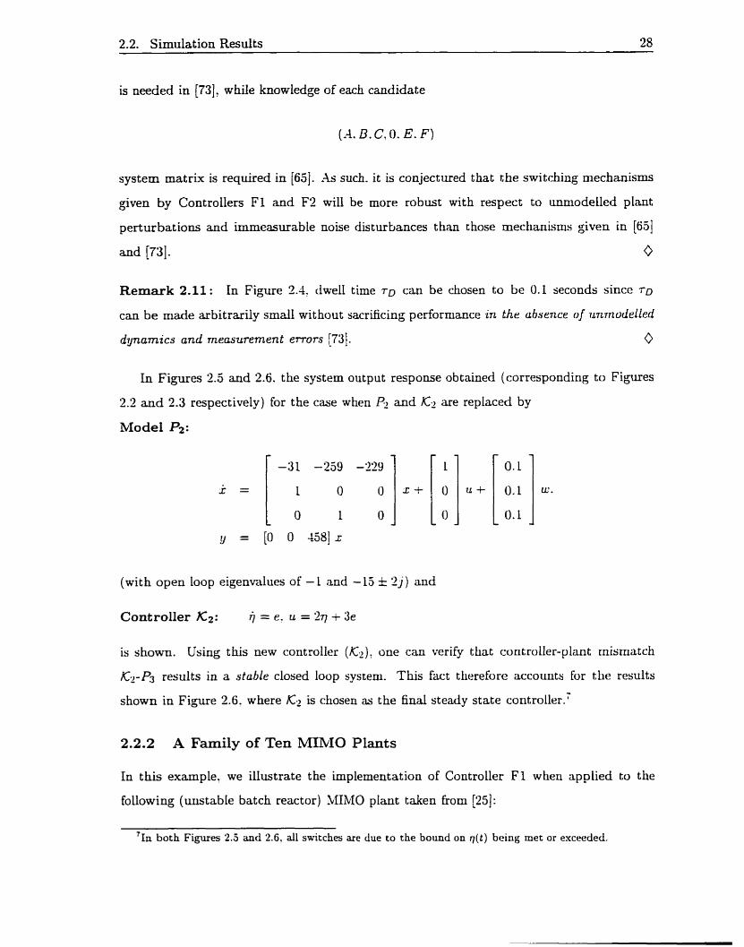
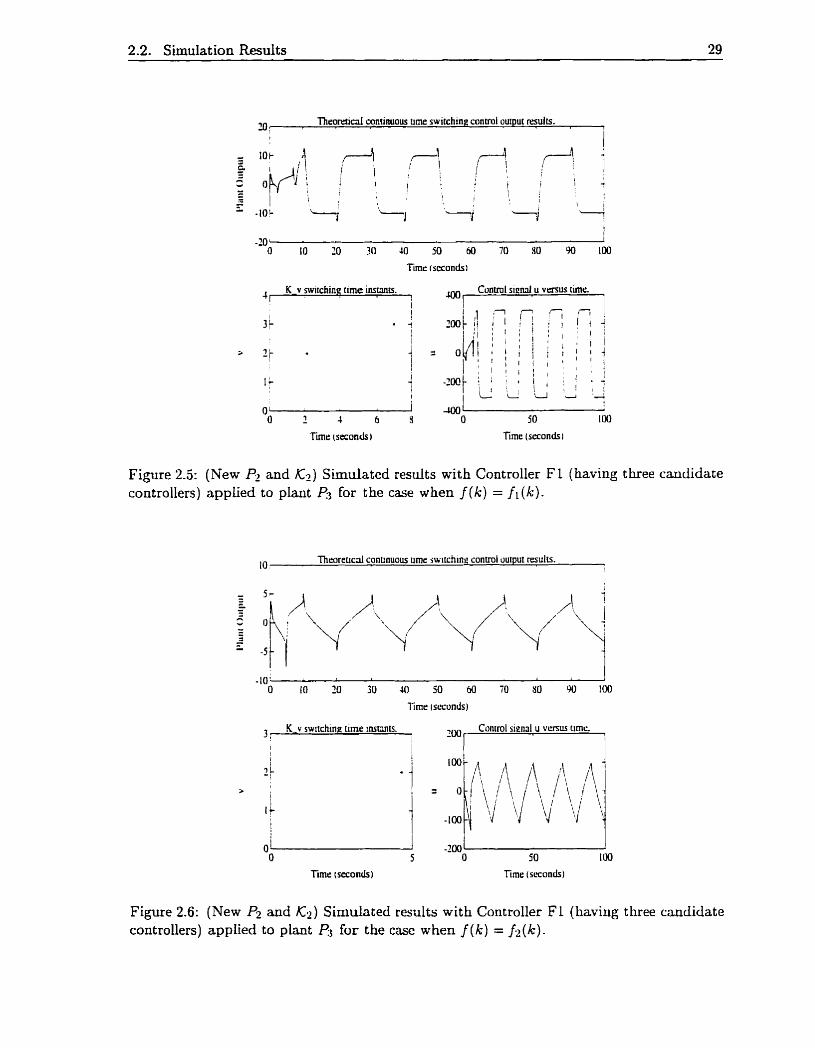
In Figures 2.5 and 2.6. the system output response obtained (corresponding to Fi,wes
2.2 and 2.3 respectively) for the case when P2 and K2 are replaced by
(wit h open loop eigenvalues of - 1 and - 15 & 2 j) and
Cont roller K2: r j=e . u = I ~ + 3 e
is shown. Using this new controller (K2): one can verify that controller-plant cnisrnatçh
&- P3 results in a stable closed loop system. This fact thcrefore accourits for the results
shown in Figure 2.6. where K2 is chosen as the final steady state controller.'
2.2.2 A Farnily of Ten MIMO Plants
In this example. we illustrate the implementation of Controller F1 when applied to the
foilowing (unstable batch reactor) MIMO plant taken froni [25]:
--
?III both Figures 2.5 and 2.6, al1 switches are due to the bound on r l ( t ) being met or exceeded.
2.2. Simulation Results 29
3: T h e o w d continuous rime switching contrai output rtrults.
I
I
l
-10 ' 1
O 10 10 30 40 50 60 70 Y0 90 100
Time (seconds i
K v switchine tirne insunrs. UIO Cunml signai u vmus timc l
Time (seconds) Timr (seconds 1
Figure 2.5: (New P2 and Kz) Simulated results with Controller F 1 (having t hree candidate controllers) applied to plant e3 for the case when j ( k ) = fi (k).
10 Thmieucd contrnuous tirne switching conuoi uutput resulrs.
Figure 2.6: (New P2 and K2) Simulated results with Controller F 1 (having three candidate controllers) applied to plant i3 for the case when f (k) = _Jr(k).
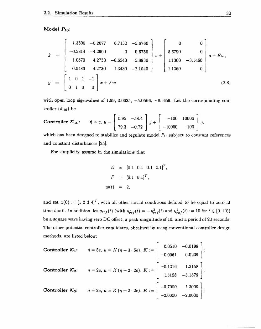
2.2. Simulation Results 30
with open loop eigenvalueç of 1.99, 0.0635, -5.0566, -8.6659. Let the corresponding con-
troller ( K I O ) be
which fias been designed to stabilize and regulate mode1 Plo subject to constant references
and constant disturbances [XI.
For simplicity, assume in the simulations that
and set x ( 0 ) := [l 2 3 4lT? witli al1 0 t h iiiitial coriditions defiiied to be eqiial to zero at
time t = O. III addition, let yre l ( t ) (with Y:e j ( t ) = -y;I>el(t) and T J ! ~ ~ ( ~ ) := 10 For t E [O. 1 0 ) )
be a square wave having zero DC offset, a peak magnitude of 10, and a period of 20 secoiids.
The other potential controller candidates, obtaiiied by using conventiorial cotitroller design
methods, are listed below:

2.2. Simulation Results 31
Controller K4:
Controller Ks :
Controller Xe:
Controller KT:
Controller Ka:
Controller Kg:
7j = e. ,u = K (77 + e). K :=
.Tj = e . u = K ( q + e ) . K:=
Using the above controllers. one can verifi that conditions iii) and iv) of .4sstimption F I
are both satisfied8. and that al1 controller-plant (Pie) niismatclies result in a closed loop
unstable system ezcep t for Controller Kn.
In Figure 3.7'. simulation results with Controller FI applied to plant PLU aiid
f (k) := 2Ok exp (k) are given. In this instance. two switches occur due to the bounds on q ( t ) and e ( t ) wtiich are
met or exceeded a t the respective times of 0.245 and 0.31 seconds. uid switcliing stops once
Controller ICs is applied. Similar to the output response shown in Figure 2.6. the above
results again emphasize and illustrate the fact that the final steady-state controller gains
may not necessarily correspond to the controller puameters associatecl witli actrid plant
Pm. It is to be noted. however, that if the closed loop systern consisting of plant P; with
contmlier parameters (G,, Hj, J j K,. L,. il.IJ) is stable if and only if i = J 1 t hen the final
controuer gains applied wiii almost aiways be ensured to be (Gi7 H,, Ji Ki ! Li: Mi).
'For brevity, the system matrices of the othcr nine plants will not be given.

2.2- Simulation Resdts 32
10, Thmrcticd contrnuous rime swirchine conuoIler resultr.
1
Tirne (seconds
Figure 2.7: Simulated results with Controller F1 (having ten candidate controllers) spplied to plant PLo with y1 (solid) and y? (dashed).
In contrast to these results. Figures 2.8 and 2.9 illustrate the output response of plant
PLo using the identical situation given for Figure 2.7. but with ControIler K3 now defined
as follows:
-1.37'76 -0.0131 ] y + [ 1.0000 0.0000 ] Controller K3: 7j = e . u = 'I -
-0.0131 -1.3753 0.0000 1 .O000
In this instance, one can verify that Assumption F1 is satisfied. and that the closed loop
system will indeed be stable if and only if Controller XII, is applied.
2.2.3 A Family of Five MIMO Plants
In this example, Controller F1 will again be applied to (2.8)" As before. assume that
'1x1 this example, howevcr, the unstable batch reactor mil1 be labelled as plant Pg.

2 -2. Simulation Resul ts 33
200 r Thasorericd caniinuous timr swttchine conuolirr resuits.
i
?O fheorerid continuous rime switchin~ conmller rcsults. I I
Figure 2.8: Simulated results with Controller F1 (having ten candidate controllers) applied to plant PLo with y1 (solid) and y3 (dashed).
Ttme (seconds)
Figure 2.9: Switching time instants with Controller F l applied to plant Pio. (Controllers which are applied due to a previous bound on ~ ( t ) or e ( t ) being met or exceeded are marked by a 'N' or an 'E' respectively.)

2.2. Simulation Results 34
and define
f (k) :=
Let al1 other initial conditions be equal to zero at tirne t = 0, and let g r e l ( t ) be a periodic
triangular wave of the form shown in Figure 2.10. For completeness, the parameters of all
candidate controllers are listed in Section B. 1.
As one can verify, Assumption F1 is satisfied aud al1 controller-plant (Ps) mismatches
result in a closed loop unstable system. In Figures 2.10 and 2.1 1. the output response as
well as the switching time instants of the closed Ioop system are given: here. al1 switclies are
due to bounds on e ( t ) being met or exceeded. Simi1a.r to the predicted t heoreticd results.
Controller ICs is also selected correctly (after approximately 0.6 seconds).
2.2.4 A Farnily of Unstable SIS0 Plants
In this last exampIe, consider the respective set of unstabIe plants aiid controllers given by
[34, pg. 1102]

2.2. Simulation Resuits 35
Time r seconds i
6 ! K v switchine time insrnu.
l
Figure 2.10: Reference signals & ( t ) (solid) and y&(t ) (dash-dotted) (top plot): and switching time instants with Controller F1 applied to plant Pi (bottom plot).
Throretical continuou iimr swrrchinr contmller rcsulis. 10
-10 ' I
5 10 15 10 15 30 35 40 45 50
Time isecondsi
Figure 2.11: Simulated output response with Controlier FI (having five candidate con- trollers) applied to plant Ps with 91 (solid) and y2 (dashed).
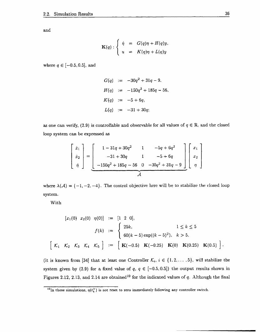
2.2. Simulation Results 36
and
where q E [-0.5.0.510 and
as one can verify, (2.9) is controllable and observable for dl values of q E R. alid the closed
loop system can be expressed as
where X(A) = {-1, -2. -4). The control objective here will be to stabilize the closed loop
sys t em.
With
[q(O) 4 0 ) q ( O ) ] := [l 2 O]!
(it is known froni [34] t hat at least one Controller Ki, i E { 1.2. . . . . 5 1, will stabilize the
system given by (2.9) for a fixed value of q, q E [-0.5.0.51) the output resiilts showri in
Figures 2.12, 2.13, and 2.14 are obtained1° for the indicated values of q. Although the final
loin these simulations, r l ( t k ) is not reset to zero inimcdiatcly follom-ing any controller switch.
2.2. Simulation Results 37
Theoreficl continuou iimr switching conrrollrr resulls. 1
7 Swirching tirne instants of controller K v. - I 1
Timc (seconds)
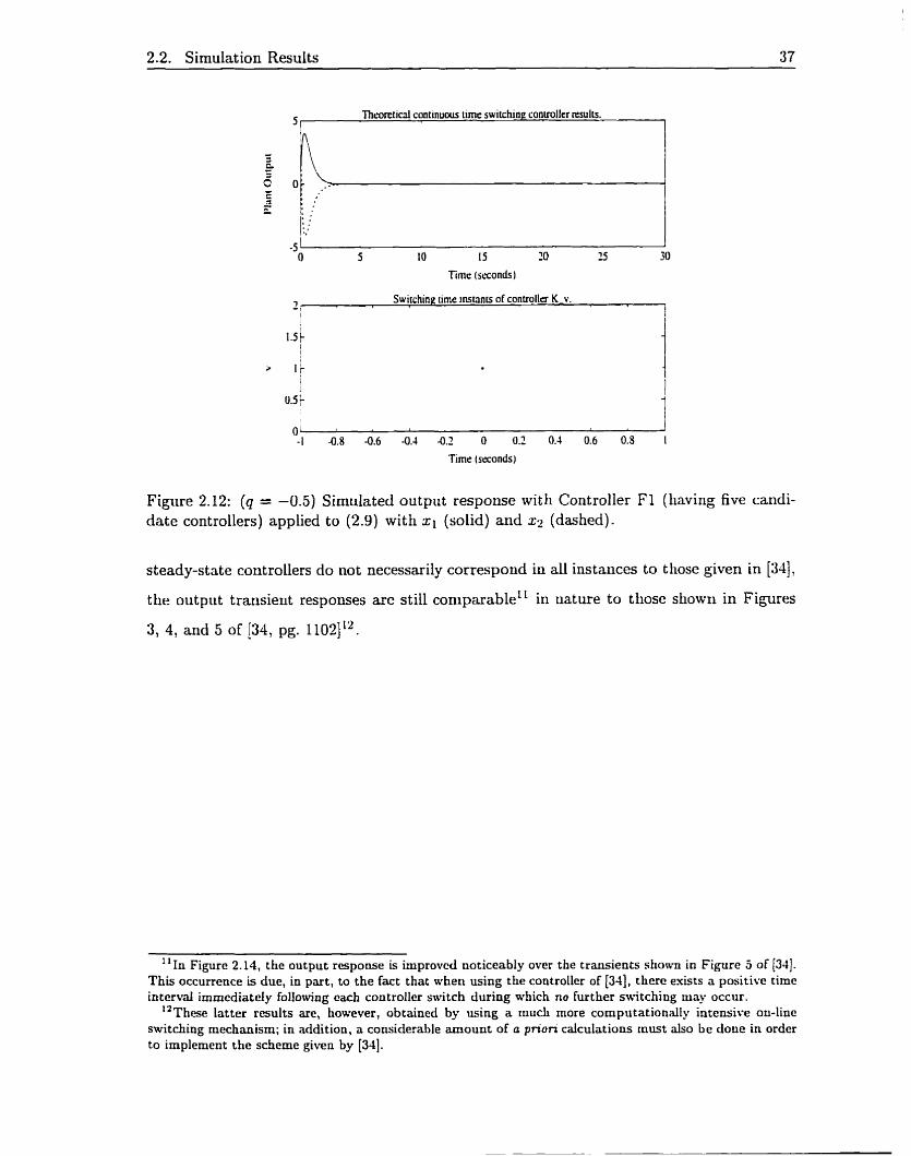
Figure 2.12: (q = -0.5) Simulated output response with Controller F1 (havirig five candi- date controllers) applied to (2.9) with xi (solid) and x2 (dashed).
steady-stote controllers do not necessarily correspond in al1 instances to those given in [34]_
the output transient responses are still coniparableii in nature to those showri in Fi y r e s
3, 4, and 5 of [34, pg. 11021".
"In Figure 2.14, the output rcsponse iç improvcd noticeably over the transients shown in Figure 5 of 13.11. This occurrence is due, in part, to the fact that wben using the controller of [34], there exists a positive time intervd immediately follotving each controller switch during which no further switching ruay occur.
''These latter results are, however, obtained by using a much more cornputationally intensive on-line switching mechanism; in addition, a considerable amount of a prion calculations rriust also be done in order to implement the scheme given by 1341.
2.2. Simulation Results 38
4 Swiichine t h e insrrints of controller K v.
l
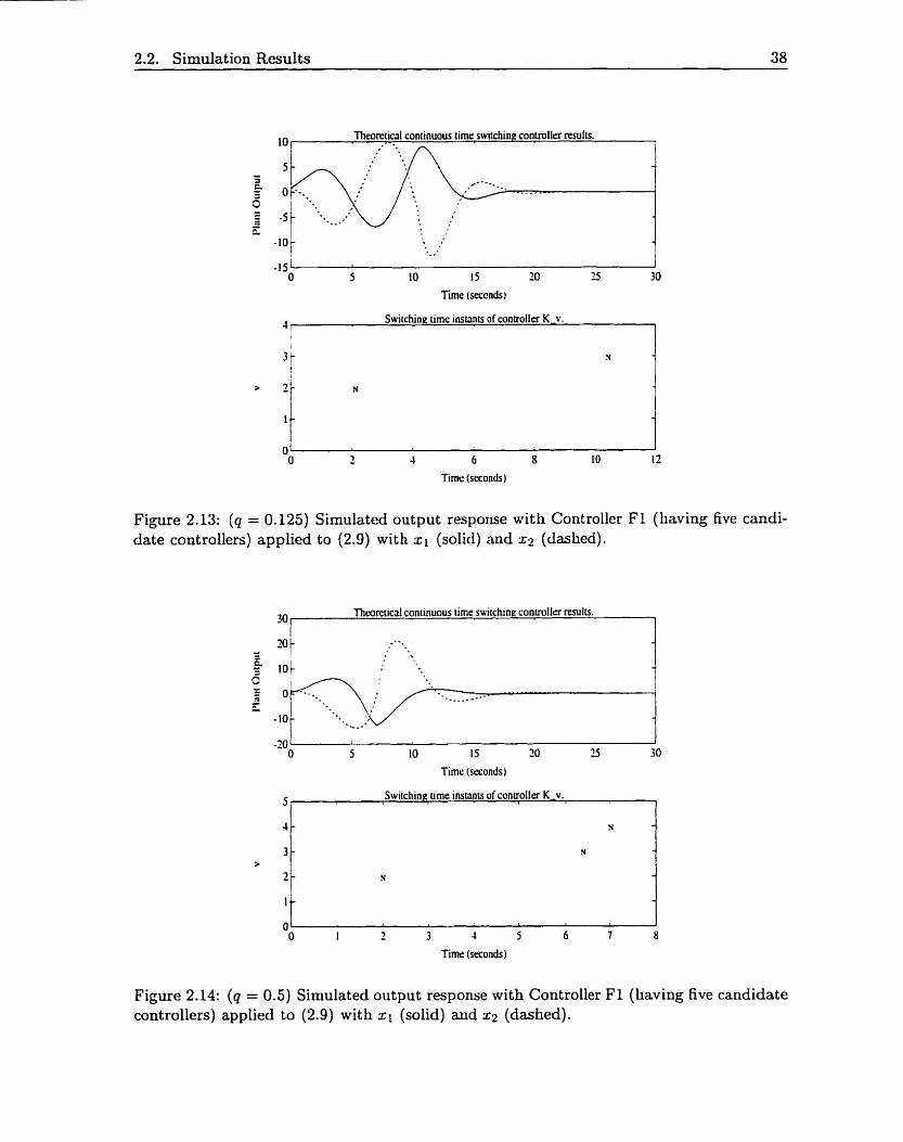
Figure 2.13: (q = 0.125) Simulated output response with Controller F1 (having five candi- date controllers) applied to (2.9) with X I (solid) and s* (dashed).
30 Theoreticai continuous tirne switchinp: conmller mlts.
I 1
-20 ' 1
O 5 10 15 70 3 30
Timr (seconds)
5 Swiichinp lime mlants of conuoIlrr K-v.
1
Timr (seconds)
Figure 2.14: (q = 0.5) Simulated output response with Controller F1 (having five candidate controllers) appIied to (2.9) with xi (solid) and x2 (dashed).

Chapter 3
Adaptive Stabilization of LTI
MIMO Systems
Using the methods and techniques developed in Chapter 2. we now propose a new stabi-
k i n g adaptive controller for the class of first order strict ly proper SISO LTI systerns. and
for the general class of finite dimensional strictly proper !vZI?vIO LTI systerns considered in
[54], [61], and [62]. Xs in Chapter 2. the controller is potentially cyclic in nature. and the
emphasis will be to provide a robust switching niechanisrn which is insensitive to bounded
piecewise continuous disturbances w ( t ) and which attempts to provide an acceptable tran-
sient response; the switching mechanism proposed here. tiowever. is sinipler in nature t han
that given in [61]. and it does not require a prelirninary identification period as given in
[621
3.1 Adaptive Stabilization of First Order LTI SISO Systems
In this section, we again utilize the switching mechanisni given in Section 2.1 to stabilize
adaptively (in the sense that z ( t ) -t O as t + zc and [r uIT E C, with w( t ) = 0. and [x
,uIT E Lm with w( t ) # O and UJ E L,) the following fint order SISO system:
(3. la)
(3. l b)
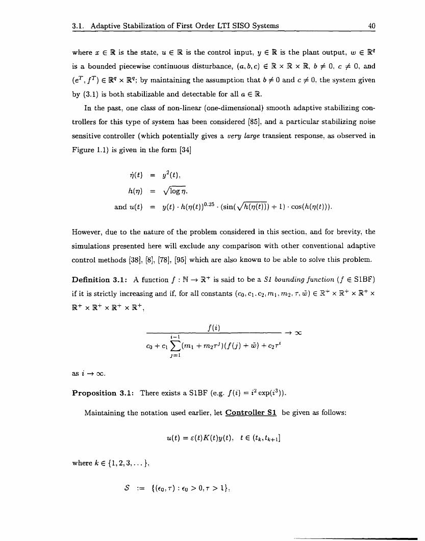
3.1. Adaptive Stabilization of Fkst Order LTI SIS0 Systemç 40
where x E R is the state. u E IR is the control input, 9 E W is the plant output, w E R4
is a bounded piecewise continuous disturbance, (a, b, c) E R x R x R? b # O: c # 0, and
(eT. f T, E R4 x Rq; by maintaining the assumption that 6 # O arid c # 0' the system given
by (3.1) is both stabilizable and detectable for ali a E R.
In the past, one class of non-linear (one-dimensionai) smoot h adaptive stabilizing con-
trollers for t his type of system has been considered [85]: and a particular stabilizing noise
sensitive controller (which potent ially gives a uery large transient response, as O bserved in
Figure 1.1) is given in the form [34]
Howe . .
!ver, due to the nature of the problem considered in t his section, and for brevity, the
simulations presented here will exclude any cornparison wit h ot her convent ional adaptive
control methods (381: (81, (781, [95] which are &O knowo to be able to solve this problem.
Definition 3.1: A furiction f : Ri + Ri is said to be a SI bounding junction (f E SLBF)
if it is strictly increasing and if. for al1 constants (ca' cl. Q: m 1 , rns: T , W ) E Ei x Bi x Rf x
Rf x R' x IRi x IR+,
asi-kx.
Proposi t ion 3.1: There exists a SlBF (e.g. f ( i ) = i' exp(i3)).
Maintaining the notation used earlier, let Control ler S1 be given as follows:
where k E {l, 2 ,3 , . . . },
S := {(eo,r) : €0 > OJ > 1)'

3.1. Ada~t ive Stabilization of First Order LTI SIS0 Systems 41
K ( t ) = , € 1 . . i = ((k - 1) mod 2) + L. t E ( t t . tk ; i ]?
t1 := 0, and where. for each k 2 2 such that tk- 1 # X. the switching time tk is defined by
i) t > t k - l : and if t his minirnuni exis ts t k :=
ii) I y ( t ) ( = f (k - 1)
l m O t herwise
with f E SlBF. Label Assumption SI to be
Here, the restrictiori that 1 y(0)l < f (1) is required in order to ensure once agairi that
the switching time tk is well defined for Controller S1. As well. Controller SI works by
monitoring plant output y ( t ) in an a t tempt to detect instability. Following each controller
switch, and similar to the results presented in [LOl]. the sign of K is clianged. and gain E is
increased with the goal of using high gain output feedback to stabilize (3.1).
Remark 3.1: Consider the SISO system (3.1): where (a, 6. c) E X x R x R. b $ 0 , c # 0.
and K := { K i : K2): then for almost al1 (E& T) E S.
Lemma 3.1 : Consider the first order SISO plant (3.1) with Controller S1 applied at
tirne t = 0, and assume that the controller [lever stops switching; let w ( t ) be a piecewise
continuous signal with w E Cm. and let sign(bKjc) = -I for one j E {1'2}. Then with k
3.1. Ada~t ive Stabilization of First Order LTI SIS0 Systems 42
sufliciently large such that ((k - 1) mod 2) + 1 = j and
the following properties hold for al1 t E (tr. t i+l] (with 1 2 k : ((1 - 1) mod 2) i L = j ) :
wliere (ci, C . e: 6, c6) E R+ x RT x Ri x Pi x B' x 8' are constants independent of
I and i r ( t r ) .
Proof: The proof follows upon first observing that
for d l 2 k' ( ( 1 - 1) mod 2 ) + 1 = j : hence. there exists a constant X E R' such that
for 1 > k. ( ( 1 - 1) mod 2) + 1 = j : t 3 0.
On defining
it therefore now foilows that
and thus that
3.1. Ada~ t ive Stabilization of First Order LTI SIS0 Systerns 43
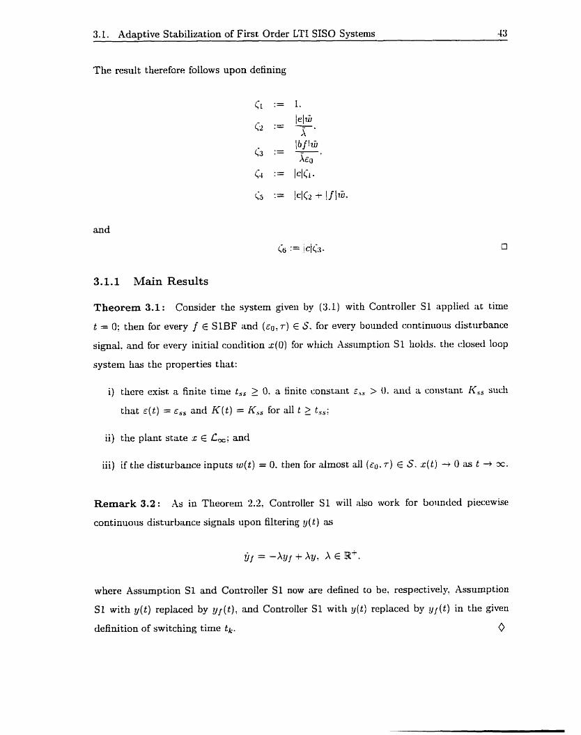
The result therefore follows upon defining
3.1.1 Main Results
Theorem 3.1 : Consider the system given by (3.1) with Controller S 1 applieti at time
t = 0: then for every f E SlBF and ( E ~ : r) E S. for every bounded continuoiis disturbance
signal. and for every initial condition ~ ( 0 ) for which Assiimption S1 iioids. the closeci loop
system lias the properties that:
i) c h r e exist a finite time t,, 1 0. a finite constant E,, > O. aiid a constant f<,, such
that ~ ( t ) =E,, and K ( t ) = Kss for al1 t 2 t,,;
ii) the plant state r~ E Cs; and
iii) if the disturbance inputs ur(t) = 0. tlien for almost al1 ( ru . T ) E S. r(t) i O as t + s.
Remark 3.2: A s in Tlieorem 2.2. Controller S 1 will also work for boiinclcd piecewise
continuous disturbance signals upon filtering y ( t ) as
where Assumption S l and Controller S1 now are defined to be. respectively. Assurnption
S1 with y ( t ) replaced by yy / ( t ) ' and Controller S1 with y ( t ) replaced by y l ( t ) in the given
definition of switching time t k . 0

3.2. Adaptive Stabilization of LTI bîTbIO Systems 44
3.1.2 Simulation Results
To demonstrate the potential t r a i e n t improvement that might be attained by iisi~ig The-
orem 3.1. consider the system (3.1) with
In Figure 3.1. the output response obtctined iising Controller S1 is shown. Similady. iising
identicai controller parameters with
(c .u .6 .e . f) := (I.1.1.0.1).
~ ( 0 ) := 1.
and ~ ( t ) := 0.25 sin(100t).
the output illustrated in Figue 3.2 is obtained. In both instances. these resiilts compare
favourably when contrasted with the respective outputs shown in Figues 1.1 and 1.2. where
a peak overshoot greater than 311000 in magnitude. and closed Ioop i~istability. respectively
result.
3.2 Adaptive Stabilization of L T I MIMO Systems
In t his section, the gencrd problem of adapt ively stabilizing the finite dimensiorial strictly
proper (stabilizable and detectable) PVIIMO LTI system given by
is examined, where z E Rn is the state, E W m is the control input. !j E Rr is the plant
output, and ul f Rq is the disturbance. The candidate feedback controllers which will be

3.2. Adaptive Stabilization of LTI MIMO Systems 45
d r Theoretid coniinuous tirne switchrng conuollrt results.
3 1 Switchine rime instants oi conuolla K=K-V.
1
Tirnç i seconds I
Figiire 3.1: ( w ( t ) := O ) Simulated results of g ( t ) witli Controller S1 applied to (3.1) .
15, Tharericd continuous time swnchine conuollrr results. 7 l
-3
O 1 4 6 Y 10 12 14 16 18 10
Time c seconds)
3 r Switchine time Insranri of conuolla K=K v. 1
I
Timr: (seconds )
Figure 3.2: (w(t ) := 0.25sin(100t)) Simulated results of y ( t ) witfi Controllcr S 1 applied to (3.1).

3.2. Adaptive Stabilization of LTf MIMO Systems 46
considered are of the form
Similar to Section 2.1? in the discussions which will follow, we do not necessarily assume
that n, A, B, C, E, or F are known. and we do not restrict X(A) C E-.
Preliminary definitions and results which are needed before proceeding are given as
follows.
Definition 3.2: A function f : W -+ 22' is said to be a S2 bounding fmct ion (f S2BF)
if it is strictly increasing and if. for al1 constants (CO. ci. mi. m7. T. 15) E BT x R- x Rf x
Wf x Ri x R'.
CO + cl x(n, i- m 2 i J ) ( f ( j ) i W)
Proposition 3.2: Tliere exists a S2BF (e.g. f ( 2 ) = 2 e x p ( i g )).
Definition 3.3: ([92. pg. 441) X set D is dense in W ifB = W. where v is the closureofD.
(i) { h ( i ) : i E W} is dense in ~ ( " ~ g ~ ) ~ ( ~ ~ g ~ ) for a hxed d u e of gi E NU (O}: and
(ii) for h ( i ) :=

3.2. Adaptive Stabilization of LTI P v ~ l O Systems 47
for constants ( T ~ 3) E IR+ x IR+.
Proposition 3.3: Given gi E N U {O). there exists a h E CTF.
Proof: Consider the situation where each element of h( i ) siiccessively examines. in a nestecl 1
fashion, each intervai [-n. ni, n E N. and tries points apart. Tlien since Il h( 1) I I = (r+q*).
and since each element of h(i) will increase in magnitude at most by one following czny given
switch. t herefore
the result foilows. [7
.As an example of how one might construct h( i ) . consider the situation wtien. for instance.
gi = 1. i E N. and rn = r = L: thcn h ( i ) c m be defined as follorvs:
3.2. Adaptive Stabilization of LTI MIMO Systems 48
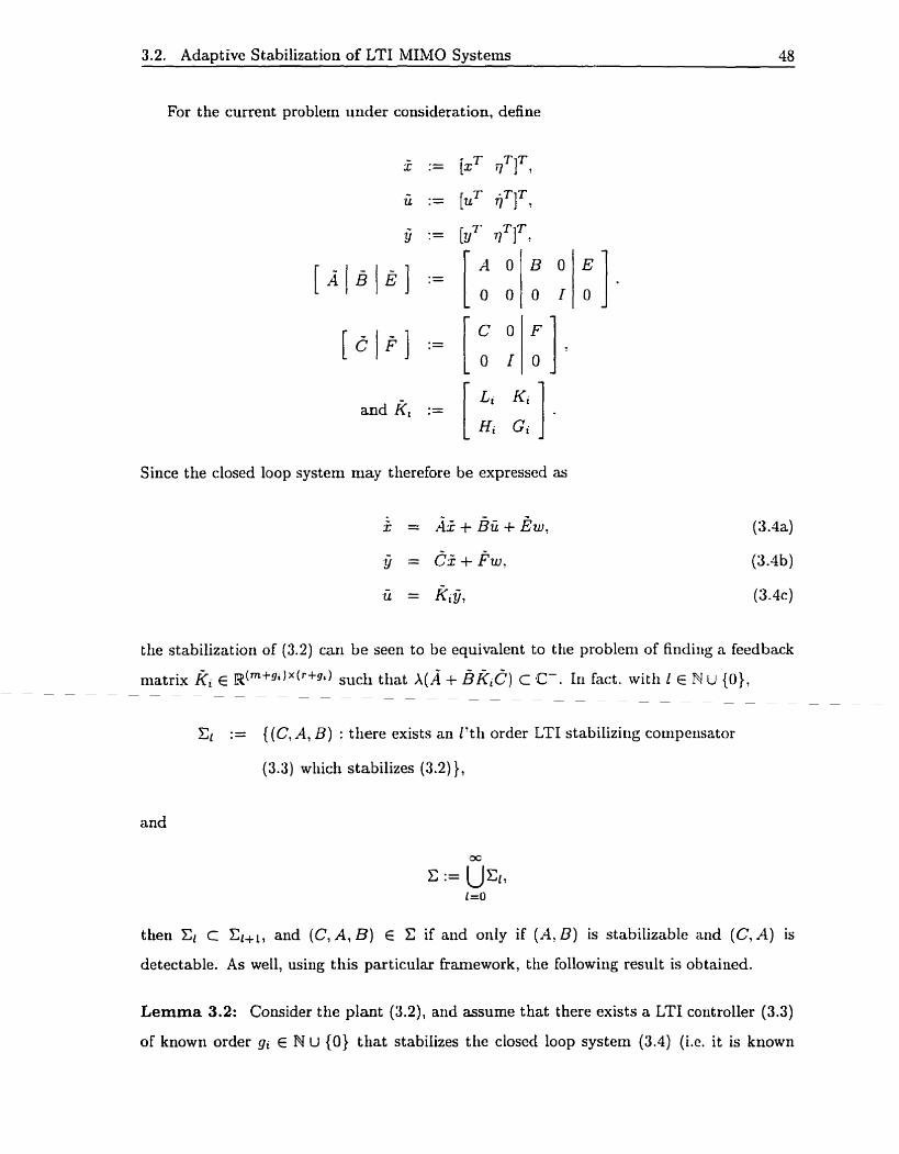
For the current problcm under consideration, define
Since the closed loop system niay tlierefore be expressed as
the stabilization of (3.2) can be secn to be equivalent to the probleni of firidirig a feedback
niatrix & E ~ ( ~ ~ g ~ l ~ ( ~ ~ g ~ ) such tliat x(A + B K ~ ~ ) C ê-. In fact: with 1 E NU {O): - - - - - - - - - - - - - - - - - - - - - - - - - - - - - -
Cl := {(C, A, B) : there exists an I't li order LTI stabilizirig comperisator
(3.3) which stabilizes (3.2) ),
and
then C l C and (C, A, B) E C if and otily if ( A , 8) is stabilizable and (C, A) is
detectable. As well, usirig t his particular frmework, t lie followiiig result is ob tained.
Lemma 3.2: Consider the plant (3.2), and assume that there exists a LTI co~itroller (3.3)
of known order gi E N U {O) that stabilizes the closed loop system (3.4) (i-c. it is known
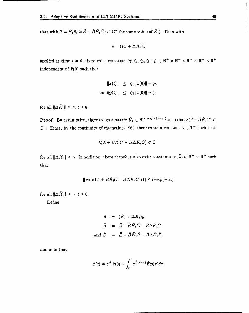
3.2. Ada~tive Stahilization of LTI MIMO Systems 49
that with ü = Kicl A(A + B K i 8 ) c ê- for some value of K~). TThen witli
applied at time t = 0, there exist constants (y,Ci,Cz,G,C4) E IR+ x Wf x WC x IRç x W+
independent of 2(0) such that
Proof: By assurnption, there exists a niatrk ki E R ( ~ + ~ ~ ) ~ ( ~ + " ) such tliat A(.<+ B R,S) c
Ce. Hence, by the continuity of eigenvalues [96], there exists a constant y E IR+ such tint
for al1 1 1 ~ ~ ~ 1 1 5 7. In addition, there therefore also exist constants (a: X) E W+ x IRt such
that
ü := (K* + AI?,)^,
À := À + B K ~ C + B A K ~ C ,
and Ë := Ë + BK*P + BAKiF,
and note that
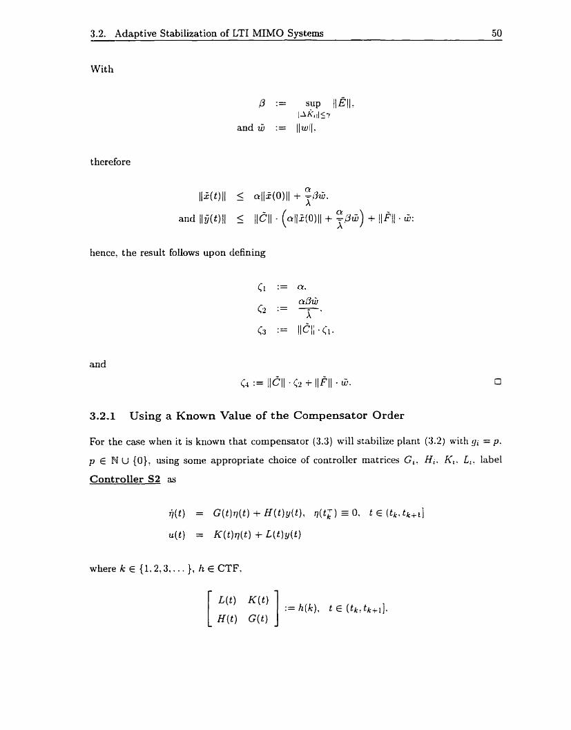
3.2. Adaptive Stabilization of LTI MIMO Systems 50
With
t herefore
arid Ilij(t)ll 5 llCll - ( ~ I I ~ ( O ) I ~ + $@lu) + !IFII . 5:
hencc, the resuit follows upon defining
c 1
(2
C3
and
3.2.1 Using a Known Value of the Compensator Order
For the case when it is known t hat comperisator (3.3) will stabilize plant (:3.2) with gi = p.
p E N U {O)' using sonie appropriate choice of controller matrices Gi. H,. K,. L,. label
Controller S2 as
where k E {l. 2 . 3 , . . . }, h E CTF.

3.2. Adaptive Stabilization of LTI MIMO Systems 51
t l := 0, and where, for each k- 2 2 such that t k - l # OC, the switching time t k is defined by
if this minimum exists
ot herwise
with J E S2BF. In additiori, let Assumption S2 be
Theorem 3.2: Consider the system given by (3.2) with Controller S2 applied at time
t = 0; then for every f E SSBF and h E CTF, for every bounded continuoiis disturbance
signal, and for every initial condition % ( O ) := [x (0 )= q ( ~ ) T ] T for which Assurnption S2 Iiolds.
the closed loop system has the properties that:
ii) the controller states rj E Loo and tlie plant states z E Lm; and
iii) if tlie disturbance inputs w( t ) = 0. tlien for alniost al1 coiitroller pararileters (G. H :
K, L ) , s( t ) -t O as t + W .
3.2.2 Using no Known Value of the Compensator Order
For the case when the order gi of a stabilizing compensator is unknown, but a lower boirnd
a E N U {O) and an upper bound y E N u {O} is known such that a 5 gi $ 7 with
a < y, ControlIer S2 can be modified such that, starting with O := a, one can search the
w ( ~ ~ ~ ) ~ ( ~ ~ O) parameter space near zero wit h a certain degree of fiiieness, arid t lien iricrease
(if necessary) the order of o by one and repeat the process with an iiicreased degree of
fineness. This idea is formalized in the following definitiori.
Definition 3.5: Given tliat a E M U {O) is a lower bound alid that 7 E N U {O} is an
upper bourid on gi such that cr 5 gi 6 y with a < y' a function h : N + ~ ( " ' + 9 ~ ) ~ ( ' + * ) is
3.2. Adaptive Stabilization of LTI MIMO Systems 52
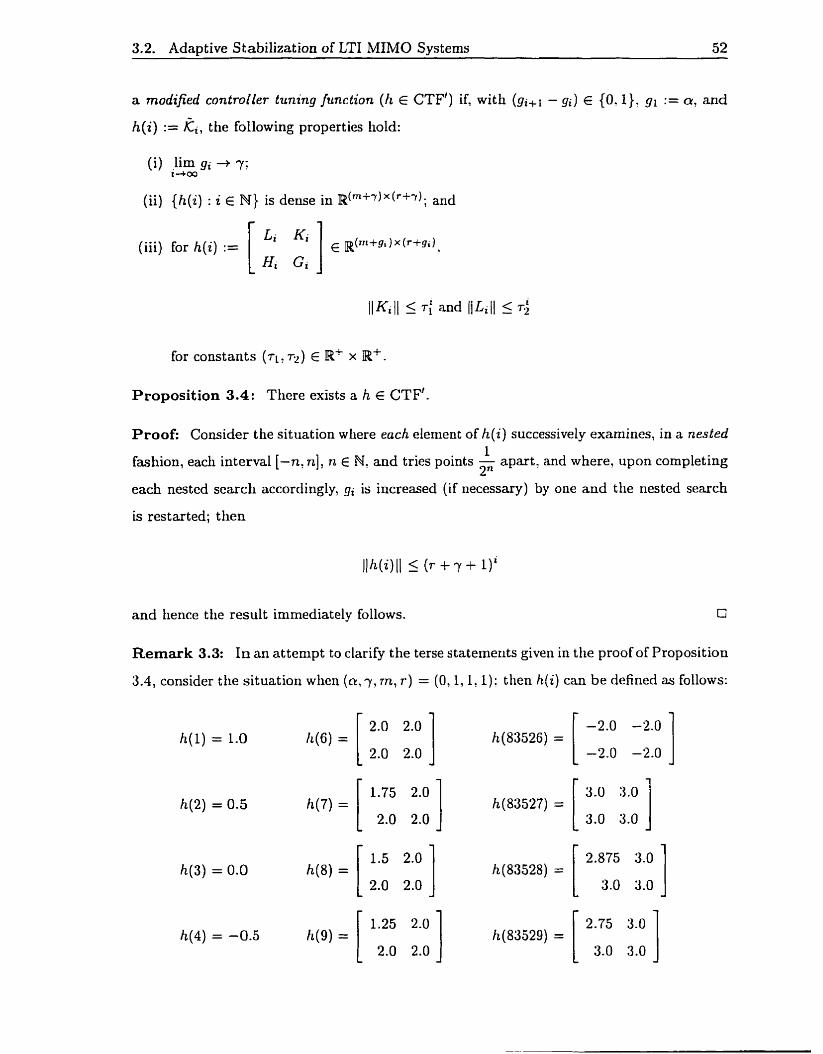
a modified controller tuning function (h E CTF') if, with (gi+[ - gi) E { O . I}. gl := a, and
h(i) := Ki, the following properties hold:
(iii) for h(i) := 1 1 R(rrl+$ 1 x (.+!hi,
for constants (ri. F ~ ) E Wç x IR+.
Proposition 3.4: There exists a h E CTP.
Proof: Consider the situation where each element of h( i ) successively examines, in a nested 1
fashion, each interval [-n'n], n E N, and tries points - apart, and where? upon completing 2"
each nested search accordingly, gi is increased (if necessary) by one and the nested search
is restarted; then
and lience the result immediately follows.
Remark 3.3: In an attenipt to clarify the terse statemerits given in the proof of Proposition
3.4, consider the situation when (a, y, m, r ) = (O, I, 1 , f ): then h( i ) can be defined as follows:
3.2. Adaptive Stabilization of LTI MIMO Systems 53
h(5) = -1.0
For the case when it is known that compensator (3.3) will stabilize plant (3.2) with
gi = p using some CY 5 p 5 y with a, y E N U {O), a < y, and using sonie appropriate
choice of controller parameters Gi? &, K,, Li, label Controller S2' to be Controller S2.
but with h ECTF'.
Theorem 3.3: Consider the system given by (3.2) with Controller 52' applied a t time
t = 0; then for every f E S2BF and h E CTF', for every bounded continuous disturbarice
sigiial! and for every initial condition *(O) := [z(OIT i I ( ~ ) T ] T for which Assumption S2 holds.
the closed loop system has the properties that:
ii) the controller states E Lm and the plant states z E Lm: and
iii) if the disturbance inputs w ( t ) = O? ttien for almost al1 coritroller paranieters (G. H:
K, L), z( t ) + O as t + m.
Here, the relative corriputational simplicity of Controllers S2 and S2' compare favourably
when contrasted, for instance, with the controllers giveu in [74], [ol]. [62]. arid [57]. 111
essence, by properly constructing f to have certain known a priori propertics: the adaptive
stabilization problem for stabilizable and detectable MIMO LTI systenis can be solved by
monitoring norrn bounds on ~ ( t ) and y ( t ) .
Rernark 3.4: As ooted in (621, if it is known a priori that there exists a gain Ki in a known
set S c ~ [ p ( ~ + g ~ ) ~ ( ' + g ' ) such that the closed loop system is stable, then one can restrict the
search of the ~ ( ~ + g ~ ) ~ ( ' + " ) parameter space to S. For example: if

3.2. Adaptive Stabilization of LTI hIIM0 Systems 54
then one can define
( EL: if ( ( i - 1) m o d p ) t L = L
E2: if (( i - 1) mod p) + 1 = 2 h(2) :=
K if ((i - 1) mod p) + 1 = p
as a controller tuning function. 0
Hence. if one can restrict the search of the Btm'S1)X(r-*) puameter space to S for
stabilizing controller parameters IC,? where
then Theorem 3.2 reduces to Theorem 2.1 with yref ( t ) := O. In this instance. f (k) need
only satisfy the property that
as i + x for al1 constants (col cl. c- ) E R' x 32- x 2'.
Remark 3.5: If w ( t ) is a bounded piecewise continuoiis signal. tlien corresponding coni-
ments equivalent to the ones given in Remark 3.2 are d s o applicable to SLieorerns 3.2 and
3.3 provided that
are additionally satisfisd for (r3: T . ~ ) E Ri x RT. (This additional restriction can always be
met by using the construction rncthods given in the proof of Proposition 3.3 and Remark
3.3.) O
3.2. Adaptive S tabilization of LTI Pc/IIPc,IO Systems 55
3.2.3 Simulation Results
Example 1: SISO Unstable Nonminimum Phase Plant
Consider the following (controllable and observable) unstable rionminimum phase SISO
plant taken Ekom [62. pg. 6041:
1 u + Ew.
wit h poles given by -2 and 0.5 kj. and zeros given by - L.5 and 0.5. Assume that the plant
is unknown. but that it is known that there exists a zero'th-order stabilizing compensator
for the system (i.e. it is known that for some d u e of L, E W. the closed loop system will
be stable with u = L i g ) . In addition. define h( i ) as
1 so that each successive i n t e d [-n. n]. n E M. is exarnined. and points , - apart are chosen.
Let
Lk, l L k . 1 1 5 and f(k) :=
20(k - 15)' exp((k - 15)"). k > 15.

3.2. Adaptive Stabilization of LTI %DM0 Svstems 56
and observe t hat the closed loop system is stable if and only if
In Figures 3.3 and 3.4, output results obtained using Controller S2 are shown for .w ( t ) :=
O and w( t ) := sin(2t) respectively. In both instances, t hese results are comparable to those
given in [61] and [62] , and. in accordance with Theorem 3.2. L ( t ) remains constant after a
finite number of switches (L,, = 2) .
For cornparison, using Controller S2 and the same initial conditions and parameters as
given for Figure 3.3. but with h( i ) defined as
the response shown in Figure 3.5 is obtained. In this iristance. L,, = 3. ami. unlike the
results presented in Figure 1 and the highly oscillatory response shown in Figure 2 of [6210
the state transient response suffers froru only an approxiniate four-fold iricrertse in peak
magnitude when compared with Fi-pre 3.3 '.
Example 2: Two Input-One Output Unstable Minimum Phase Plant
As anot her example. consider the (stabilizable and observable) unstable minimum phase
MIS0 plant [62. pg. 605)
'in [62], Figure 2 suffers from an approximace seven-fold increase in peak maguitude when conipared with Figure 1.

3.2. Adaptive Stabilization of LTI MIMO Systems 57
15 Theoretical conrtnuous tirne switching conmller renilts. 1
rot A
Tirne (seconds)
6 Switchine rime instants of conuoller L=L v.
01 I
O 1 2 3 4 5 6 7 Y
Time (seconds
Figure 3.3: ( w ( t ) := O) Simulated results with Controller S2 applied to (3.5) using (3.6) with xi (dotted), xz (dashed), x3 (dash-dotted), and y (solid).
10 [ Thmrertcal continuous tirne switchine conuoller w!ts.
Time (seconds)
6 i Switching rime m s m s of conuolIer L=L v.
Time (seconds)
Figure 3.4: (w(t) := sin(2t)) Simulated results with Controller S2 applied to (3 .5 ) using (3.6) with zi (dotted), x2 (dashed), x3 (dash-dotted), and y (solid).
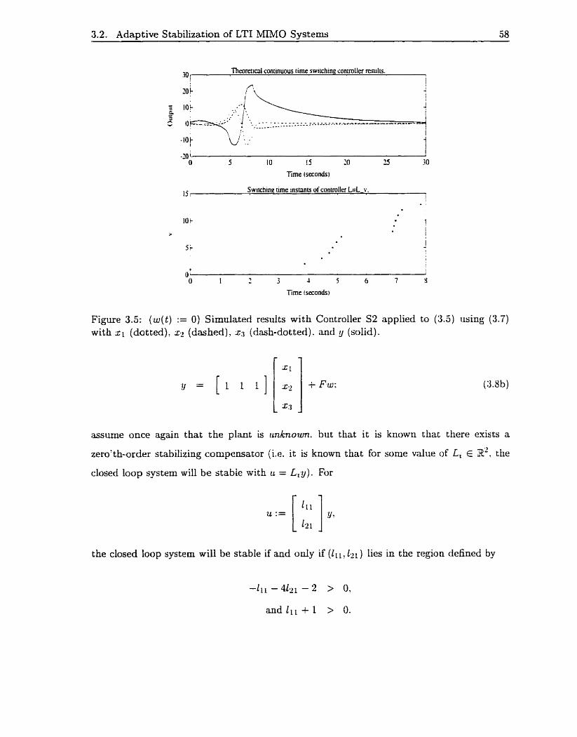
3.2. Adaotive Stabilization of LTI MIMO Systemv 58
30, T h r o ~ r i d continuous time swirchtne conmller rcsulis. 1 1
Figure 3.5: ( ~ ( t ) := O ) Simulated results with Controller S2 applied to (3.5) using (3.7) with LT 1 (dotted), z- (dashed), s3 (dash-dotted). and y (solid).
assume once again that the plant is i~nknourn. but that it is known that ttiere exists a
zero'th-order stabilizing compensator (Le. i t is known that for some value of L, E P'. the
closed loop system will be stable with u = L,y). For
the closed loop system will be stable if and only if (1 l , 1-1 ) Iies in the region defined by
-11L-412i - 2 > O.
and I l l + 1 > 0.
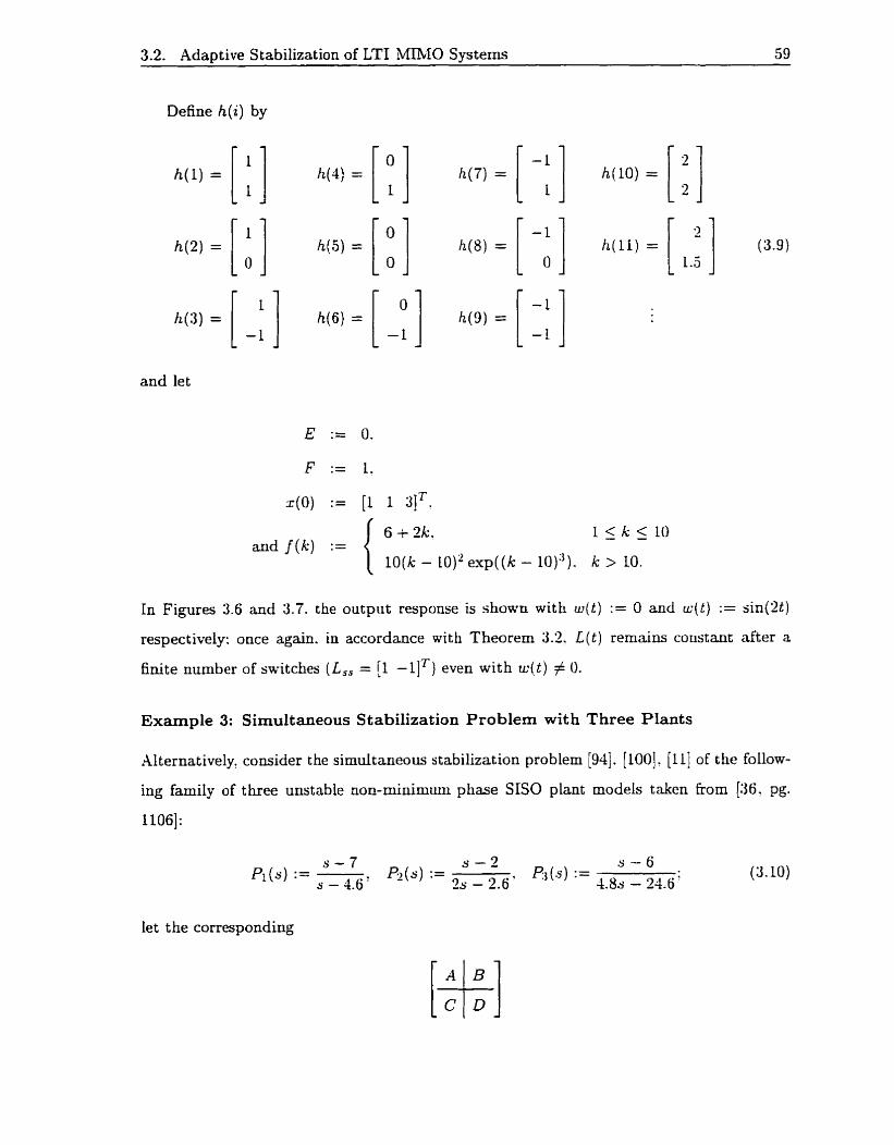
3.2. Ada~t ive S tabilization of LTI bIIhIO Systerns 59
and let
6 + 2k. l ~ k - < l O and f(k) :=
10(k - LO)' exp((k - 10)"). k > 10.
In Figures 3.6 and 3.7. the output response is shown with w ( t ) := O and u(t ) := sin(2t)
respect ively: once again. in accordance with Theorem 3.2. L ( t ) remains coustant after a
finite number of switches ( L , , = [l -llT) even with w ( t ) # O.
Example 3: Simultaneous Stabilization Problem with Three Plants
Alternatively? consider the simultaneous stabilization problem [94]. [100]: [11] of the foilow-
ing family of three unstable non-minimum phase SIS0 plant models taken Erom [36' pg.
1 los]:
S - 7 5 - 3 .S - 6 Pr ( s ) := - pi&) := P3 (s) :=
s - 4.6' zs - 2.6: 4.8s - 24.6'
let the corresponding

3.2. Ada~tive Stabilization of LTI MIMO Systems 60
Thmretid continuous m e switchinn conuolla results. 'O 1
Time (seconds )
Switchinp rime insfan~ of conuoller L=LLv. t
! 0 ;
O 0 2 0.4 0.6 0.3 I 1.1
Time (srcon&)
Figure 3.6: ( w ( t ) := O) Simulated results with Controller S2 applied to (3.8) using (3.9) with xi (dotted), z2 (dashed). xn (dash-dotted), and y (solid).
Throreiical continuous time switchine conuoller ~ . ~ ~ l t s . IO r 1
!
Tirnr (seconds)
3 Switchine timr instuits of controller L=L v.
"O 0.1 0.7 0.3 0.4 O3 0.6 0.7 0.Y 0.9 1
Time (seconds)
Figure 3.7: (w(t) := sin(2t)) Simulated resdts with Controller S2 applied to (3.8) using (3.9) with X I (dotted), xz (dashed), x3 (dash-dotted) and y (solid).
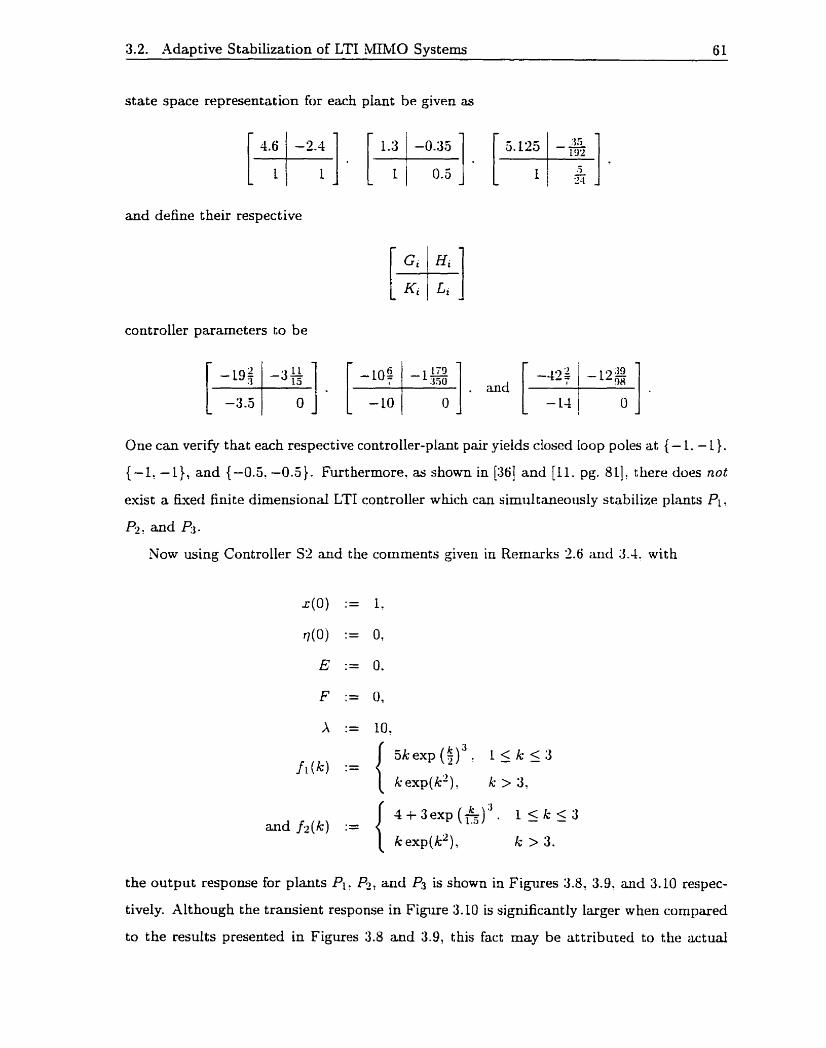
3.2. Adaptive Stabilization of LTI ~ ~ 1 0 Systems 61
state space representation for each plant be given as
and define their respective
controller parameters to be
One can veri@ that each respective controller-plant pair yields chsed Ioop poles at i- 1. - 1).
{-1: - l}, and {-0.5' -0.5). Furthermore. as shown in (361 and [LI. pg. 811: there does not
exist a Lxed finite dimensional LTI controller which can simdtaneously stabilize plants Pi
fi: and Pj.
Now using Controller S2 and the cornmentu given in Remasks 2.6 and 3.4. with
and f2(k) :=
the output response for plants Pl, Pz, and f i is shown in Figures 3.8' 3.9. and 3.10 respec-
tively. Xlthough the transient response in Figure 3.10 is significantly larger when cornpared
to the results presented in Figures 3.8 a d 3.9, this fact may be attributed to the x t u a l
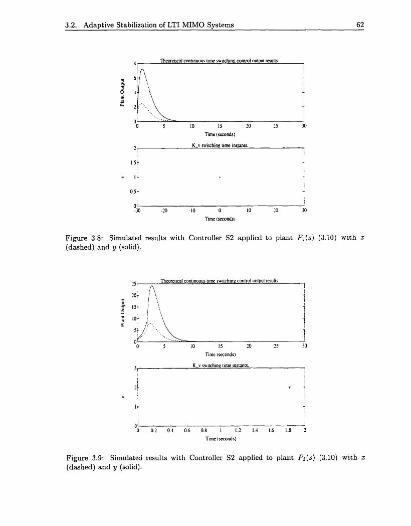
3.2. Adaptive Stabilization of LTI MIMO Systems 62
8 Tharet~cJ conrinuou urne swirching convol output resultr.
1 O' - W . -
O 5 IO 15 10 15 30
fime (seconds)
Timr (seconds 1
Figure 3.8: Simulated results with Controller 52 applied to plant Pi (s) (5.10) witli x (dashed) and y (solid).
75 Theoreiicd continuous time switching conuol ouipul raulrs.
n 1
1
Timc (seconds)
3 i K v switchine time insmts.
1
I
1
i 0 1
O 0.2 0.4 0.6 0.8 1 1.2 1.4 1.6 1.8 2
Time (seconds)
Figure 3.9: Simulated results with Controller S2 applied to plant &(s) (3.10) with x (dashed) and I/ (solid).
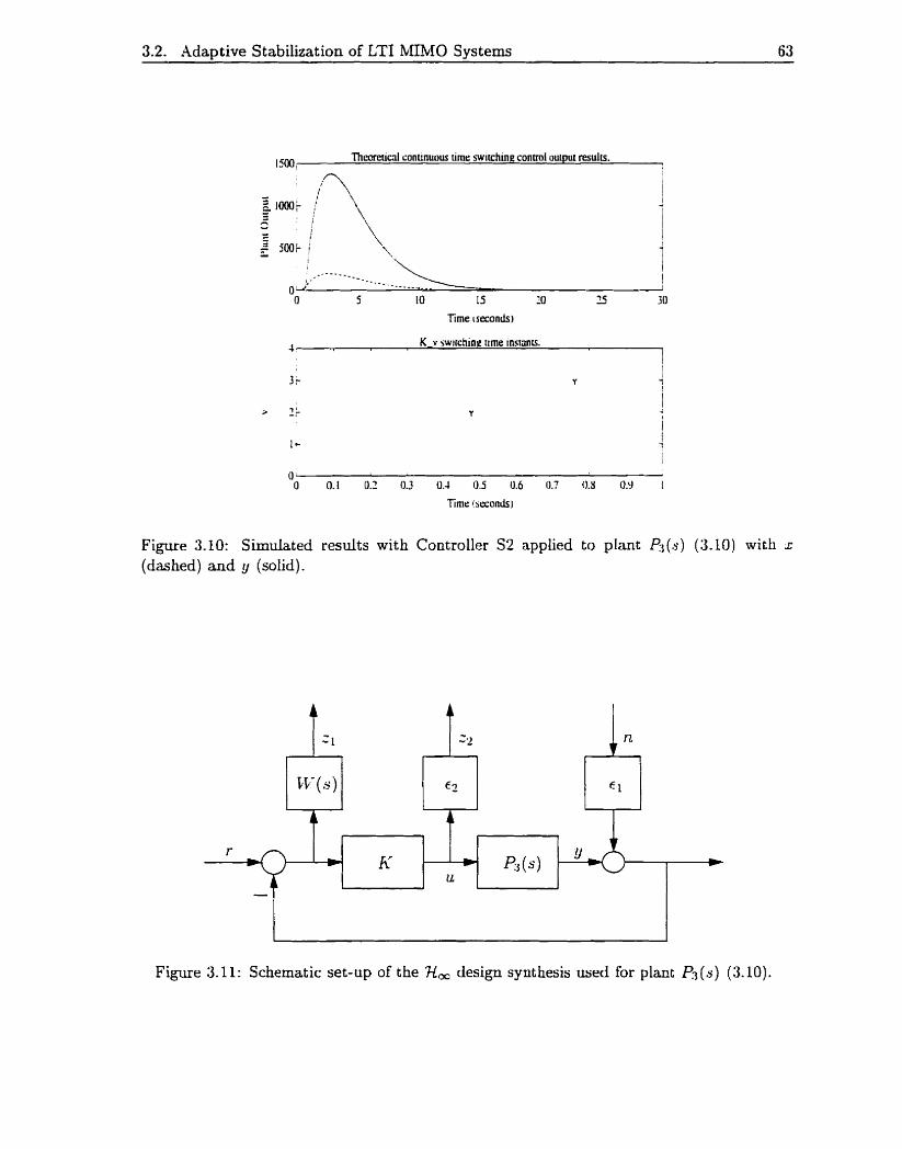
3.2. Ada~t ive Stabilization of LTI hfi%IO Svstems 63
1500, Thmerical çonunuous tirne switchine convol ouipui results. i
Time i seconds
J K v switchine lime insmts.
O' O 0.1 0.2 0.3 0.4 0.5 0.6 O.? 0 . Y Y I
Timr t seconds I
Figure 3.10: Simulated results with Controuer S2 applied to pIant P3(s) (3-10) with ;c
(dashed) and y (soiid).
Figure 3.11: Schematic set-up of the X, design synthesis used for plant P7 ( Y ) (3.10).
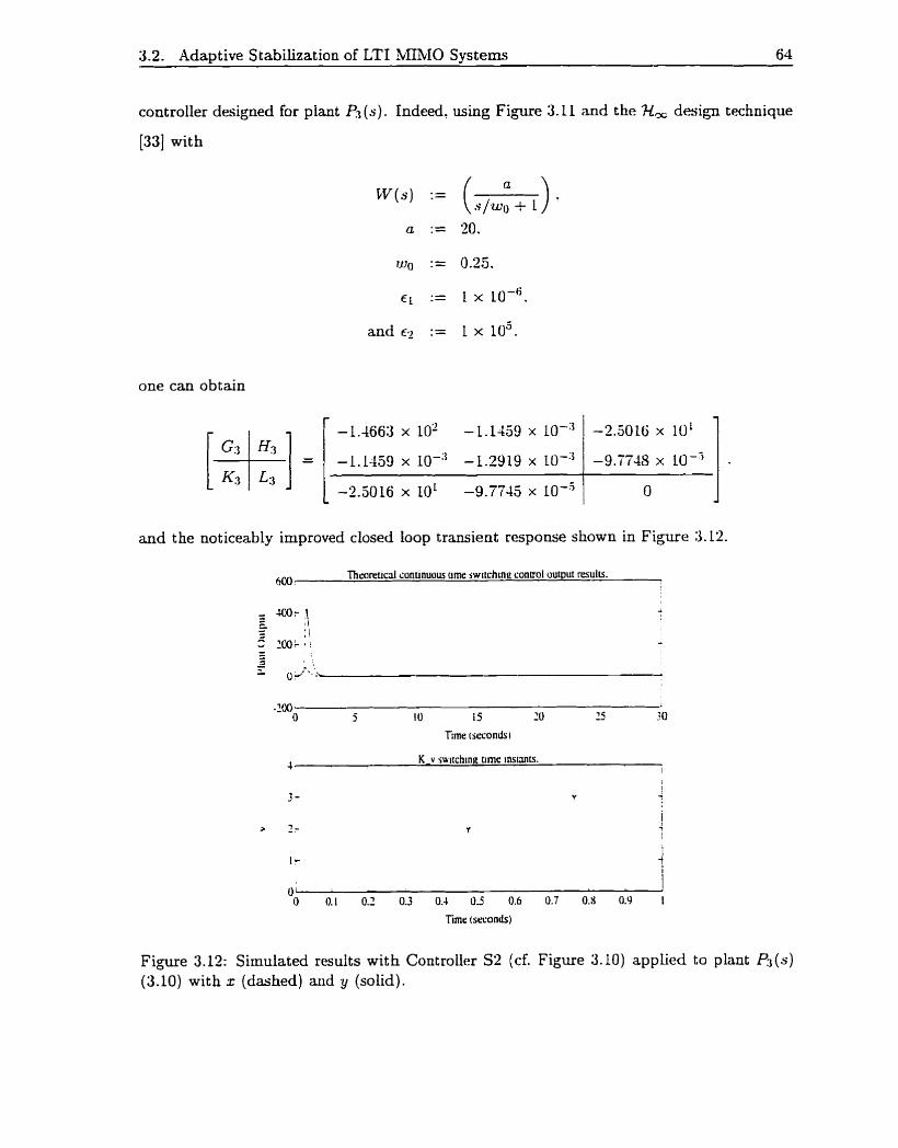
3.2. Adaptive S tabilization of LTI PViIbIO Systems 64
controller designed for plant PÎ (s). Indeed, using Figure 3.11 and the R, design technique
[33] wit h
and €2 := 1 x 10'.
one can obtain
and the noticeably improved closed loop transient response shown in Figure 3.12.
m. Thzareucal conunuous orne swiichme conuol output results.
Tirne (seconds)
Figure 3.12: Simulated resuits with Controller S2 (cf. Figure 3.10) applied to plant Pi(s) (3.10) with x (dashed) and y (solid).
Chapter 4
The Self-Tuning Robust
Servomechanism
In this chapter, the robust self-tuning controllers presented in [64], [lj]. and [16] for cases
involving both a known and an unknown estirnate of the steady-state DC gain matriu 7
will be reconsidered: as well, two riew self-tunirig proportional-integral-derivative (PID)
controllers for similar corresponding cases will also be deveroped. In an attenipt to irnprove
the output transient response, the proposed controllers now switch based upon norrn bounds
on q( t ) and e ( t ) . The results presented here ttierefore indicate that a more general controller
structure than originally given by Miller and Davison in [64] can be implemented on an open
loop stable system using a switching criterion with very Little a prioll system information.
4.1 Self-Tuning Proportional-Integral Control
Consider the finite dimensional LTI systeni given by
k = ,42+ Bu + Ew, y = Cx+ Du + Fw? e := Y r e j - y
(4.la)
(4.1 b)
(4. lc)
where x E Rn is the state, u E W m is the control input, y E Rr is the plant output to be
regulated, w E WQ is the disturbance, and e E Wr is the differcnce betweeri the specified
reference input y,,/ and the output g. Assume that m > r, that A is stable, that rL, A, B,

4.1. Self-Tuning Proportional-Integral Control 66
C' D. E. or F are not necessarily known. and restrict fief and w to be bounded piecewise
constant signals; let f E MSBF. and define 7 := D - C.4-L B. For the case wlien the
estimate of 7, T' has full row rank, let K := p. (An estirnate (n of 7 can be obtained
via rn steady state experiments outlined in [21].)
In t his section, the self- tuning ro bust servomechanism controllers considered in [64]: [ls], and [16] for cases involving both a known and an unknown estimate of the steady-state DC
gain matrix 7 will be re-examined. As in these earlier results. assunie throiiglmiit chat 7
has fui l row rank in order to form a tractable problem. and niaintain the definitions (e.g.
f E MSBF) and notation given in previous cbapters.
Definition 4.1: X function g : N + Et' is a tuning function (9 E TF) if lim g(k) = O. If A--=
fa g E TF and if there exist finite constants €0 > O and T > L so that g ( k ) = - for k E N.
rk
then define g E TF' to be a modified tuning fiinction.
4.1.1 Using an Estimate of the DC Gain
When an estimate of 7. given by T. is available. define the set of admissible controller
parameters as
Label Assumrition PI1 to be
iii) -TT+ is stable: and
€0 iv) (1 t p - D K ) . i E (1.2.3.. . . ). is invertible for Lxed p 2 O (see Remark 4.1): rL
then with a = ( j . g, p) E a. define Controller PI1 as
4.1. Self-Tuning Proportional-Integral Control 67
t l := 0 , and where. for each k 2 2 such that t k - L # X. the switching time t k is defined by
i) t > t k - ~ . and if this minimum exists t k :=
ii) 1llq(t)* e ( t ) T ] T ~ ~ = f (k - 1)
I X O t herwise.
Remark 4.1 : Given p > O and D E Rr m. then for almost d l E E 2.- and for almost d l
matrices K E Rm"', (1 + p d K ) is invertible. 0
The following results will also be needed.
Theorem 4.1 : ([48. pg. 571) Consider the singularly perturbed system given by
where ( X ~ ~ Q . E ) E RnL x Rn- x 2-. If -4;; exists. then as c i O. ni eigenvalites of (4 .2)
tend to
1 while the remaining ny eigenvalues of (4.2) tend to infinity. with the rate of -. dong the
E l
asymptotes defined by - X (A2 - ) . E
Corollary 4.1 : ([48, pg. 581) Consider the singularly perturbed system given by (4.2).
If ~2 exists. and if A. := ilii - A ~ ~ A ~ ~ A ~ ~ and AT2 axe asymptoticdly stable matrices.
then there exists an E* E Ri such that for dl E E (O, E * ) the system (4.2) is asymptotically
stable.
4.1. Self-Tuning Proport ional-Integral Control 68
Lemma 4.1: Consider the closed loop system
wit h
Assume that 1 exists (see Remark 4.1). and that -4 and - T K are both stable. Tlisu tliere
exist constants (a. P . E * ) E Xt x 32- x R- with the property that for every initial condition
and for every pair of bounded piecewise continuous reference and disturbance signals.
for é E (O.€'). t >_ 0.
Proof: To prove Lemma 4.1. observe from (4.3) that
eig(-<(p. c ) ) = e . eig(A(p. E ) )
w here
Rom the comments given in [48. pg. 481 and Corollary 4.1. there then exists an E' E R-
such that eig(A(p. E)) C C- for all E E (O. E'). Hence, by the continuity of eigenvdues, for
foced p 2 O. there exist constants (a. a) E R' x W' such that
for d l E E ( O . E * ) , t 2 0.
4.1. Self-Tuning Proportional-Integral Control 69
Define
Since
it therefore follows upon taking norms that
for al1 E E (O? E * ) , t 2 0.
Lemma 4.2: Consider the matrix
where i E {l? 2 , 3 , . . . ) and
€0 and À := A - p - ~ ~ f ~ . 7'
Assume that both A and -TK are stable: then for almost al1 T ) E S,
Proof: Since this proof closely follows the proof of Leninia 4 given in (641, only the major
necessary modifications will be provided. To proof Lemma 4.2, observe that

4.1. Self-Tuning Proport ionai-Integral Control 70
(wbich is assumed to exist (see Remark 4.1)) can alternatively be rewritten as
where Ï is a matrix whose elements are polynornials in a and the elements of K. and where
!2 is a polynomid in E and the elements of K with the property that
det [ SI - .A + ~ B K Ï C -BKÏ 1 L =- fin-r det +A
EÏC + E ~ D K
where
and since -i is a rnatrk whose elements are polynomial; of c and the elements of K. the
proof of Lemma 1.2 cao now continue using the identical method given in [W. pg. 5211. 0
Lemmas 4.1 and 4.2 ensble us to obtain the t'ollowing.
Theorem 4.2: Consider the stable plant (4.1) with D = O and with Controller PI1 applied
at time t = O: t hen for every 5 E n. for every bounded constant reference and disturbance
signal, and for every initial condition r (0 ) := [x(o)= q ( ~ ) T ] T for which Xssumption PI1
holds. the closed loop system has the properties that:
i) there exist a finite time t,, 2 O and a finite constant es, > O such that e ( t ) = es, for
al1 t 2 t,,:
ii) the controller states E Cs and the plant states z E C,: and
iii) if the reference and disturbance inputs are constant signals and g E TF', then for
almost all ( Q , T ) E S, e ( t ) + O as t -P oc.

4.1.2 Using no Estimate of the DC Gain
For the situation when no estimate of 7 is available? define the set of admissible controller
parameters as
- fi .- .- {( f , g , pl LI) : / E MSBF. g E TF'. p 2 O? U E Etmxrn and is nonsingular}
and let S' := {(Q, T , U) : €0 > 0, T > 1: Lr E IRmXm and is nonsingular};
with b = (f, g, p, U) E 6 and Assumption PIl' defined to be
i) il~(0)Il c f (1);
ii) Ile(0)ll < f (1): and
iii) (1 + ~ I - D K ) , i E (1: 2 , 3 , . . . } ' is invertible 7'
label Controller PI1' as
rt
for fixed p ': O (see Rernark 4.
where k E {1.2,3,. . . },
t := 0, and where, for eacli k 2 2 such that t k - L # cc: the switcllirlg time ta is defiried by
min t 3
i) t > t k - 1 , and if this minimum exists t k :=
ii) 11[~(t)~ e ( t ) T I T ~ ~ = m - 1)
30 otherwise
with
K ( t ) = UWi, z { 2 s i = ( ( k - 1 ) r n o d s ) + l , t E ( tkl tk+i] .

4.1. Self-Timing Proportional-Intemal Control
An explicit method for constructing K, := UW, for the case wlien m 2 r is given in [55]
which ensures t hat - W W , is stable for at least one j E (1 , 2, . . . . s ). s E N.
Using the same method as shown in the outline of the proof of Lemma 4.2, and following
exactly the proof given in [64, pp. 521-5223, the following result can also be obtained.
Lemma 4.3: Consider the niatrix A(p7 B , K) defined in (4.4) wliere A is stable and p 2 O
is fixed; the11 with K := { K I : j E (1,2, . . . . s)} (an explicit met hod for calculating K, is
given in [55]), for almost al1 ( r o , T. U) E Sf7
Theorem 4.3: Consider the stable plant (4.1) with D = O and with Controller P I l f applied -
at time t = 0; tlien for every b E fio for every bounded constant refererice and disturbance
signal, and for every initial condition z(0) := ( ~ ( 0 ) ~ qt(0)*IT for which Assuniptiori PI1'
holds, the closed loop system has the properties that:
i) there exist a finite time t,, 2 O, a finite constant es, > 0. and a matrix K3, such that
~ ( t ) = es, and K( t ) = Kss for al1 t 2 t,,;
ii) the controller states 71 E Cm and the plant states z E Lm; and
iii) if the reference and disturbance inputs are constant sigrials and g E TF1' then for
almost ail (eO, r ,U) E S ' , e ( t ) + O as t + m.
4.1.3 Simulation Results
To illustrate th2 effect of this new switching mechanisni on a system's potential closed loop
transient response, consider the following MIMO plant taken Erom [64, pg. 5171:
4.1. Self-Tuning Proportional-Integrd Control 73
which has a DC gain given by
and a nominal transfer function rnatrix (Le. with E = O ) given by
Assume that the following estimate of T is known:
let
and set dl controller-plant initial conditions to be equal to zero at time t = O. For t his
example. do not reset controller States q ( t ) to be equal to zero immediately followiug any
controller switch.
In Figures 4.1 and 4.2. the output resporise of the closed Ioop system is shown with
Controllers P2 1141 and PI1 applied respectively. As can be seen' in Figure 4.2. a l controller
switches are due to norm bounds on e ( t ) being met or exceeded: however, although the
actual switching time instants shown in Figures 4.1 aud 4.2 are relatively close to each
other, a substantially improved transient response occurs in Figure 4.2. This result can be
attributed to the fact that Coatroller PI1 now uses an additional norm bound ( J l e ( t ) JI) in
rui attempt to detect instability.

4.1. Self-Tuning Proport ional-Intepal Control
Theoreticai conunuous tirne swiiching contmllrr output responsr.
Tmi: (seconds)
5 . Switchine ttrnc instants of the wplid controlla.
1
!
Figure 4.1: Simulated results of y1 (solid) and y2 (dashed) with Controller P2 [I-l] applied to (4.5).
10 Themucd çontmuous urne switchine controller autput mponse. i
Figure 4.2: Simulated results of g1 (solid) and y2 (dashed) with Controller PI1 applied to (4.5).
4.2. Seff-Tuning Proportional-Integral-Derivative Control 75
4.2 Self-Tuning Proport ional-Integral-Derivat ive Control
In t his section, pract icd self- tuning proportional- integral-derivat ive ( PID ) controllers of the
form [6]
will be considered when applied to the system given in (4.1) for situations involving both a
known and an unknown estimate of the steady-state DC gain matrix 7. A s in Section 4.1.
assume throughout that T has fùll row rank in order to form a tractabie problem.
Note that for constant parameters p. c. €1, Q. :V. and K. the closed loop system formed
by augmenting (4.1) toget ber wit h (4.7) c m be expressed as
where (see Remark 4.2)
4.2. Self-Tuning Proportional-Integral-Derivative Control 76
Furthermore, here? we consider "derivative" terms of the form
- P
and not of the form
since, as noted in [6, pg. 71, the reference signal yrel(t) is normally piecewzse constant in
nature. As well, the proposed first order filter (d(s)/y(s)) is used in order to limit t lie noise
sensitivity produced by the derivat ive action in any pract ical situation.
4.2.1 Using an Estimate of the DC Gain
For the self-tuning PID controller using a known estimate of 7, given by j. define the set
of admissible controller parameters as
Q P ~ D := {(f, 9.914~ p. 1V) : f E MSBF, g E TF'. gl E TF', E TF'. p 2 O. N > O } ,
iii) -'TF is stable; and
iv) (1 + p % ~ ~ + % N D K), i E { I l 2 ,3 , . . . }. is invertible for (eu, ri co2. 3) E S x S Tl T$
and for fixed p >_ O, N > O (see Remark 4.2).
With o p r ~ = (f, g,gi , g2, p, N) E ClprD, define Controller PIDl as follows:
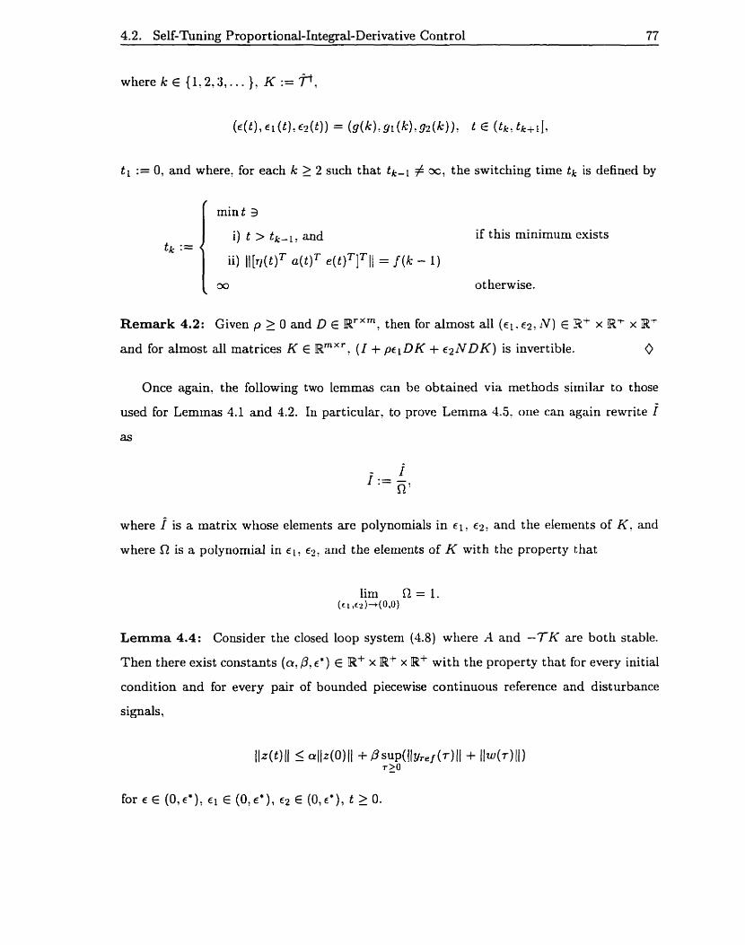
4.2. Self-Tuning Proportional-Integral-Derivative Control 77
where k E {1!2.3 ,... }, K := ?!
t l := 0 , and where, for each k > 2 such that tk- l $ OC, the switching time t k is defined by
I -. ot herwise.
Remark 4.2: Given p > O and D E Etrxrn: then for almost al1 ( E ~ . Q , N ) E IRr x Rt x Rt
and for alrnost d l matrices K E !Etmx Y (1 + pi D K + E ~ L V D K ) is invert ible. 0
Once again, the following two lemmas can be obtained via methods siinilar to those
used for Leminas 4.1 and 4.2. Iu particular. to prove Lemma 4.5' one can again rewrite f as
where Î is a matrix whose elements are polynomials in €2: and the elements of K' and
where fi is a polynomial in € 1 : €2: and the elements of K with the property that
Lemma 4.4: Consider the closed loop system (4.8) where A and -7-K are both stable.
Then there exist constants (a' 8, es) E R+ x R+ x W' with the property that for every initial
condition and for every pair of bounded piecewise continuous reference and disturbance
signals,
IIz(t) I I 5 alIz(o) I I + f l s u ~ ( l l ~ r . f ( ~ ) T ~ O I I + I l w ( ~ ) I l )
for E E (O,E*), € 1 E (O, E * ) , E* E (O, E * ) , t 3 0.
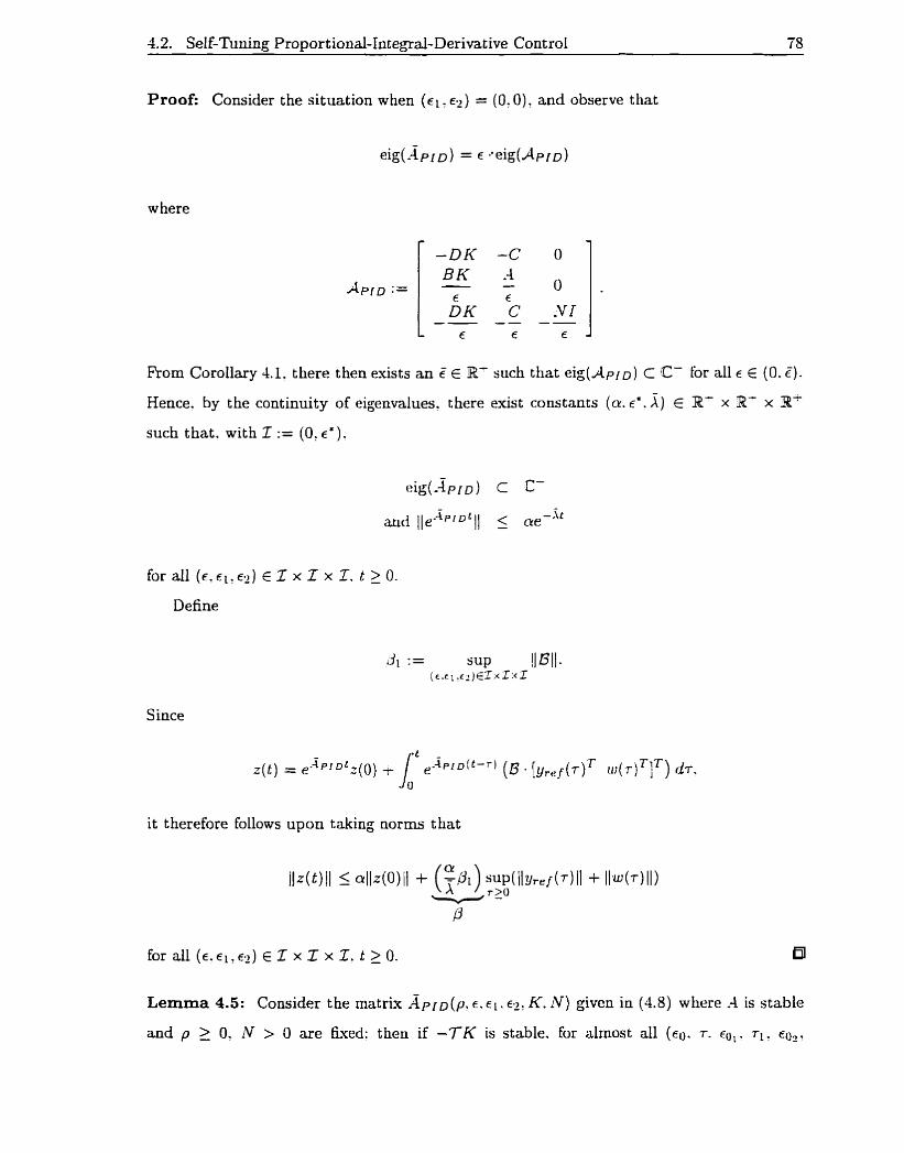
4.2. Self-Tuning Proportional-Integral-Derivative Control 78
Proof: Consider the situation when ( € 1 , E-) = (0: O ) , and observe t hat
eig(-xPrD) = c baeig(AprD)
w here
Rom Corollary 4.1. there then exists an E f R' such that eig(APID) C C- for ail E E (O. Z).
Hence. by the continuity of eigenvalues. there exist constants (o. 6'. 1) E W- x B- x R I
such that. with 1 := (O? cl) .
it therefore foIlows upon taking norms that
for dl ( E . E ~ , E ' ? ) Z x Z x 2. t 3 O. 6l
Lemma 4.5: Consider the matriv Apro(p. el. € 2 : K. N ) given in (4.8) where -4 is stable
and p 2 O. iV > O are h e d : then if - T K is stable. for almost al1 (q. T. col. ri, ~ 0 ~ .

4.2. Self-Timing Proportional-Integral-Derivative Control 79
These results enable us to obtain the following.
Theorem 4.4: Consider the stable plant (4.1) with D = O and with Controller PIDL
applied at time t = O ; then for every op [ * E f l P I D : for every bounded constant reference
and disturbance signal. and for every initial condition -(O) := [Z(O)' O(0)T a ( 0 ) ~ 1 ~ for
which Xssumption PIDl holds, the closed loop system has the properties t hat:
i) t here exist a finite time t,, 2 O and constants (eSs: E , ~ , ~ , E,.$- j E R- x R' x R' such
that ~ ( t ) = E , ~ . ~ l ( t ) = E ~ ~ ~ . c 2 ( t ) = for al1 t 2 t,,:
ii) the controller states q. a E 15,. and the plant states ~c E C,: and
iii) if the reference and disturbance inputs are constant signais and g E TF'. gl E TF'.
g2 E TF'. then for almost di (Q. r-60,. q . c o 2 . -) E S x S x S. e( t ) -t O as t + x.
4.2.2 Using no Estimate of the DC Gain
For the self-tuning PID controller using no known estimate of T. define the set of admissible
controller parameters as
let Assumption PID 1' be Assumption PID 1 with condition (iii) rernoved.
With o'prD = (f > g, 91 g2:p. 1V. U ) E Q ( P I D : define Controller PIDI' as

4.2. Self-Tuning Proportional-Integral-Derivative ControL 80
where k E (1 2.3. . . . ).
t := 0: and where. for each k >_ 2 such that t k - 1 $ X. the switching time tk is defined by
O t herwise
wit h
K ( t ) = UbViv,, i E {l. 2 . . . . ..s). i = ((k - 1) mod s ) + 1. t E (tt. t k - L ] .
An explicit method for constructing the K, := CrCVj for the case when m > r is given in
[55] which ensures t hat -TKj is stable for a t least one j E { 1.2.. . . . s } . s E N.
Lemma 4.6: Consider the matrix d p l D (P . é. c 1. € 2 . K. LV) given in (4.8) wbere -4 is stable
and p > O. iV > O are k e d : then with K := {h; : j {l. 2.. . . . s)}. for almost al1 (eu r.
eo,? TI: E O ? . - :L I ) E S x S x Sr'
Theorem 4.5: Consider the stable plant (4.1) with D = O and with Controller PIDL'
applied at time t = O: then for every o>plD E O'pro. for every bounded coustant reference
and disturbance signal, and for every initial condition r (0) := [z(O)' rl(0)T a(0)'lT for
wliich Assumption PID1' holds. the closed loop system has the properties that:
i) there exist a finite time t,, 2 0' a matrix Kss, and çonstaots (c,,'a ,,,. a,,?) E Rf x
W+ x R+ such that K ( t ) = Kss? c ( t ) = ers, 8 1 ( t ) = e,,,. e2( t ) = es,, for d l t 2 t,,:
ii) the controiler states 77: a E Coc? and the plant states x E L,; and

4.2. Self-Tunine: Pro~ortional-Integral-Derivative Control 51
iii) if the reference and disturbance inputs are constant signals and g E TF'. g~ E TF',
g2 E TF'. then for almost al1 (cor .eo, . r l : ~ ~ ~ . i l , Li) E S x S x S': e(t) i O as t i p.
Remark 4.3: If LI # O and/or if yref(t) or w ( t ) are bounded piecewise constant reference
and disturbance signals. 'hen Theorems 4.2. 4.3. 4.4. and 4.5 can be rnodified. as in Tlieorem
2.2, by letting X E 8'. by defining
ef := -Xef + Xe.
and by switching based upon norm bouods on (rl(t)T a( t )= e1(t)'lT or [rl(t)T a(tlT ef(tjT
~ ~ ( t ) ~ ] ~ (assuming that el(0) < f ( 1) and uf (0) < f (1)). 0
In Theorems 4.4 and -4.5. relatively little a priori plant information and on-Iinc conipii-
tation is required in order to successfully apply either Controller PID 1 or Controller PID 1'
to a potentially unknown (not necessarily strictly proper) b1IMO open loup stable systcm.
In essence. with n. A. B. C. D. Er. or F potentially unknown. but with 'T having full row
rank and X(A) C C-. al1 proposed controllers will alrnost always provide asymptotic error
regdation and disturbance rejection with y,,f and w bounded constant signals. Furthcr-
more. in an attempt to reduce the transient tuning response. the switching criterion riow is
based partially upon the norm bound of e ( t ) .
These facts therefore compare favourably when contrasteci. for instance, witti the SIS0
results outlined in j1021. [SI. [35]. [o]. [do]. (71. and with the (strictly proper) M M 0
results given in [83]. [88]: [89]. [53]. [AS]. [52]. More specifically. it is assumed that rn = r
(wit h each decentralized control agent meauring only one plant output and manipuhting
only one plant input) and tliat an accurate mode1 representation is available in [83]: tliat
on-line manual tuning of the proportional-integral controllers occurs in [88]: that m = r.
rn 5 TL, and that input-output decoupling (in the sense of 132. pg. 6521) occurs in [89] and
[45]; that rn = r and that diagonal decentralized control occurs in [53]; and that diagonal
dominance occurs in [52]. Moreover' the scheme of [83] admits the possibility of Iiaving to
first design m! c~ntrollers~ and 3 s based on a t heorem and two heurist i d .
Remark 4.4: Consider the situation when

4.2. Self-Tuning Proportional-Integrai-Derivative Control 52
i) (f 1. f3) € CMSBF:
Then, similax to Remark 2.4, Theorems 4.2. 4.3. 4.4. and 4.5 will also hold for al1 botrnded
piecewise constant reference and disturbance signais with D not necesszily equal to z e n
and with the switching time t k given by
, min t 3
i) t > t k -L : and if t his minimum t'xists
ii) Ilq(t)ll = f i ( k - I ) and/or (4.9)
This occurs since. with Lxed admissible controller parameters. Controller PIDL can be
expressed as
[:] = [; - N I " [ [ u ] - [il !/+ [;]fief.
in its most generd form (4.10). As well. in this instance. witii p := O and € 2 := 0. (4.9)
reduces essentially to the origind definition of switctiing time t k given for Controllers 2 and
2' in [64]. 0
Remark 4.5: Theorems 4.4 and 4.5 are both equally valid for the (PI) case when E - := O
(see Theorems 4.2 and 4.3) and for the (ID) case when p := 0. 0
Theorems 2.4 and 4.5 are also valid for self-tuning PID controllers of the form [9. pg.
2221

4.2. Self-Tuning Proportional-Intemal-Derivative Control 83
where (b . N ) E Ri x P'. This follows since the closed loop system may be expressed as
(4.8) where
and
Furthermore. in this particular case. the comments given in Remarks 4.3. 4.4. and 4-21 also
hold true.
4.2.3 Simulation Results
Example 1: Two Input-Two Output System
Consider once again the systern given by (4.5). As before. assume that the fbllowing estimate
of 7- is known:
let f (i) be given by (4.6). with
1 O g ( i ) := - 2i ?
( t ) := [-2 - 2IT.
and set ail controller-plant initial conditions to be equal to zero at time t = O.

4.2. Self-Tuning Proport ional-Integrd-Derivat ive Control 84
Using Controller 2 defined in [64], the output respoose shown in Figure 4.3 is obtained.
For coniparison, the results obtained by applying Controller PID 1 wit h
p := 1. and N := 1 are given in Fiogre 4.4; in this case, al1 initial conditions are also set to
be equal to zero a t time t = 0' the states of q ( t ) are not reset to zero after each controller
switch, and the same rnodified strong bounding function f ( 2 ) as defined in (4.6) is used.
As can be seen, in t his instance, the output transient response of Figure 4.4 is not iceabiy
improved over that shown in Figure 4.3. (The one switch which occurs at 0.475 seconds in
Figure 4.4 is due to the bound on [T(t)T a ( t ) T ] T . ) For further cornparison. using similar
initial condit ions and parameter functions/values (unless o t herwise noted) as in Figure 4.4'
the plant output obtained using Controller PID1' and Controller PID1 is sliown in Figures
4.5' and 4.6 respectively. In Figure 4.5,
0.2 - ((k - 1) niod 6):
and the cyclic switching action as suminarized in Table 4.1 is iniplenietited2; for Figure
Table 4.1: Summary of the cyclic switching behaviour used for Figure 4.5.
' ~ e r e , no estimatc of 7 is assumed to be knonn. 2 ~ n this case, fivc cycles through each of the six possible feedback matrices are requircd before switching
stops; once again, the states of q ( t ) are not reset to zero aftcr each controller switch.

Theoreticai conunuom urne switching conuoller output respnse.
i
J r Switchine time instants o f the applird conmlla.
I I 1
Figure 4.3: Simulated results of y1 (solid) and g? (dashed) with Controller 2 given by Miller and Davison [64] applied to (4.5).
O r Theorcrical continuous urne swirchinn conuoller outpur rrsponsr.
I Switchine unw insmts of ~hc mpliai conuoIler.
1
l
01 i O 0.05 0.1 0.15 0.7 0.3 03 0.35 0.4 0.45 0.5
Tirne (seconds)
Figure 4.4: Simulated results of y1 (solid) and yz (daslied) with Controller PIDl applied to (4.5).

4.2. Self-Tuning Proportional-IntegraI-Derivative Control 86
4.6, p is set to be equal to zero (with q( t ) not reset to zero immediateIy following the one
controller switch). Note that in Figure 4.5: switches which are due to the bound on e ( t )
or [r)(t)T a(tlTlT axe denoted by an 'E' or a .X' respectively. while in Figure 4.6. the one
switch is again due to the bound on [q(t)= a ( t ) T ] T .
Remark 4.6: For a two input-two output system. the six possible feedback matrices are
and
Example 2: Four Input-Four Output Building Temperature System
As anot her example. consider the (four input-four output) partial decentralized temperature
control problem of a multi-zone building [29] described by
x = . ~ L c + B u + E ~ T ~ ~ ~ ? (4.1 la)
y = Cx. (4.11b)
For cornpleteness. matrices A, B. C. and E are given in Section 8.2. As one can verify.
X(A) C @- [29: pg. 121 and
has full r a d .
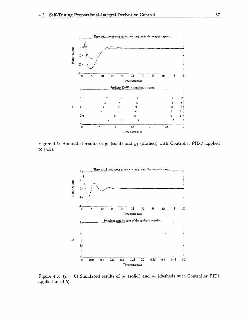
4.2. Self-Tuning Proportional-Integral-Derivative Control 87
Thco~ical conrinuous urne switchine conuolIer ourput femme. 1
-31 {
O 5 10 15 10 -5 30 35 U) 15 5 0
Time c seconds)
3 , Fdback K=W v switchine insrana.
1
6 r K x Y Et I
Y Y Y
1r Y Y Y E l Y Y Y i :1
2 LE e Y E E l b Y Y Y E d
UL J
O 0 5 I l .j 7 15 3
Timr istronds i
Figure 4 3 : Simulated results of y1 (solid) and y? (dashed) with Controller PID1' applied to (4.5).
u, Thearcticri1 connnuous trmc switchine conual1er ouiput mponsc. 1
3 i Swiichine tune instants of the ripplird conuollcr. I
01 j
O 0.05 0.1 0.15 0.2 0.25 0.3 0.35 0.1 0.15 0.5
Timr !seconds)
Figure 4.6: (p = O ) Simulated results of y1 (solicl) and y2 (dashed) with Controller PEDL applied to (4.5).

4.2. Self-Tuning Proportional-Integral-Derivative Control 88
Assume that an estimate of 7, given by
is available, and let
and K := T-' ;
tiere, y,, ( t ) and 6Tmt(t) represent respectively tlie perturbed reference (tenlperattire) aiid
disturbance inputs about riominal values sel and Tm(. With q( t ) not reset to zero aftcr each controller switcli and Controller PIDl applied
a t time t = 0, and using zero initial coriditions and the parmieter values in (4.12): the
output response shown in Figure 4.7 is obtained. We note that two switches occur at
approximately 0.518 and 2.244 minutes due to tlie bound on [q( t )T ~ z ( t ) ~ ] ~ . In additiou.
since K # ( -CA-'B)- ' and dTmt(t) # 0, one tlierefore can also conclude that the coiitroller
is robust. Alternatively, upon applying the h e d integral controller [29] given by
with identical initial conditions, references, and disturbances, the discernibly more oscilla-
tory response stiown in Figure 4.8 is obtained.
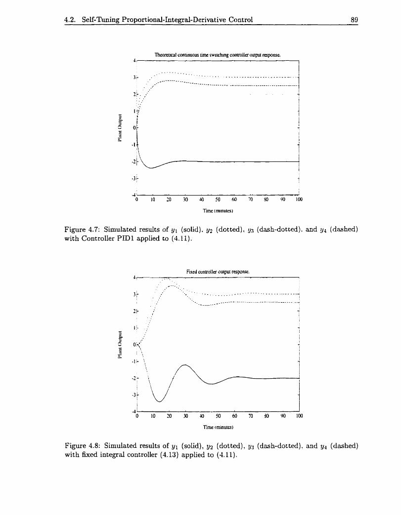
4.2. Self-Tuning Proportional-Integral-Derivative Control 89
Thmretic;il conunuous urne switcfiing controllri output response. J r
Time (minutes I
Figure 4.7: Simulated results of y1 (solid). y2 (dotted). (dash-dotted). and y4 (dashed) with Controller PID1 applied to (4.1 1).
Fued controller output respanst!.
Figure 4.8: Simulated results of yl (solid), y:! (dotted), y~ (dash-dotted). and y4 (dashed) with fixed integral controller (4.13) applied to (4.11).

4.2. Self-Tuning Proportional-Integal-Derivative Control 90
Example 3: Four Input-Four Output Furnace System
For a final example, consider the situation when an estirnate of 7- is assunieci to be knowri.
and w hen ( filtered) ControIler PID 1 ( using (4.10)) is applied to t Lie following niodel-reduced
(four input-four output) furnace systern taken originally from [gl . pg. 1991'':
with X( ,AR) C (C- and D R f O. Since
one c m therefore verify that
(Le. K := I ) satisfies condition iii) of .4ssurnption PIDL.
In Figure 4.9. the output response of the closed loop system iising Controller PID 1 is
shown wit b
3 ~ o r brevity, the systcrn matrices uscd arc giwn in Section B.3.

4.2. Self-Tuning Proportional-integral-Derivative Control 91
and ail initial conditions of the controller
t = O. Here. one controller switch occurs at
and plant defined to be eqiial to zero at time
0.352 seconds (due to the norm bound on [s( t )T
a(t)=IT being met or exceeded), and. similar to the earlier results. q ( t ) is not reset to zero
immediately foliowing this switch. Moreover: due to the relatively poor estimate of 7 which
is used for t his particular class of reference and dist urbance signals (117 - j l l = 1.33). and
due to the fact that
one can therefore also conclude that Controller PIDZ is indeed robust in nature.
Thmrrtrcal conunuous urne switching conuolla output rrsponse. IO.
Figure 4.9: ( D R # O ) Simulated results of (solid), y* (dotted). y3 (dash-dotted), and y,l (dashed) with (filtered) Controller PID 1 applied to (4.14).
Finally, we include for completeness Figure 4.10. which shows the output response4
'1x1 this case. no further controller snitches occur for t > 0.
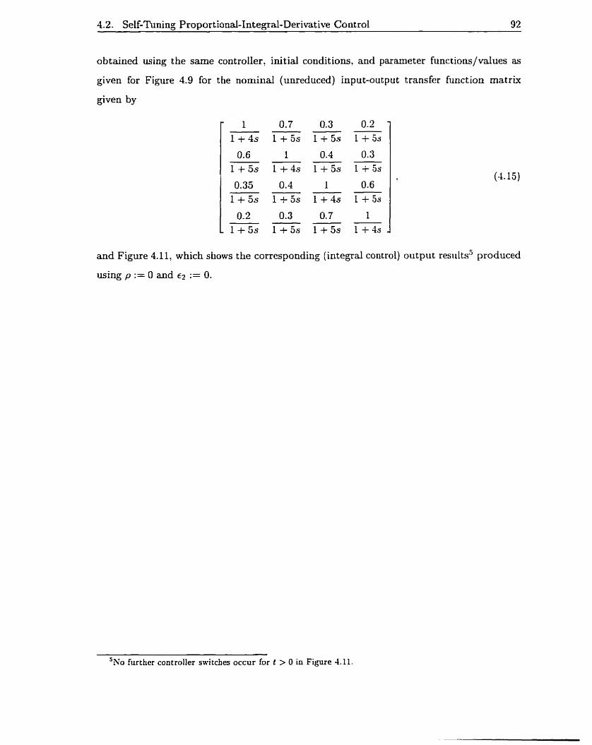
4.2. Self-Tunino Pro~ortional-Intemal-Derivat ive Cont rol 92
obtained using the same controIIer, initial conditions, and parameter funct ions/vaIues as
given for Figure 4.9 for the nominal (unreduced) input-output transfer funct ion rnatriv
given by
and Figure 4.11, which shows the corresponding (integral control) output resiilts5 produced
using p := O and €2 := 0.
'NO furthcr controller switches occur for t > O in Figure 4.11.

4.2. Self-Tuning Proportional-Integral-Derivat ive Control 93
Theoretical continuous urne switching contmiIer output response. OS,
Figure 4.10: Simulated results of (solid), y;! (dotted), y3 (dash-dotted), and 94 (dasbed) with Controller PIDl applied to (4.15).
ThmreticaI conunuous timr switching conûotlrr output rtrponsr. 0.5 r
8 10 12
Time (seconds)
Figure 4.11: ((p, E Z ) = (0, O)) Simulated results of y1 (solid), y2 (dotted), y3 (dash-dotted), and y4 (dashed) with Controller PIDl applied to (4.15).

Chapter 5
The Self-Tuning Servomechanism
with Control Input Constraints
Similar to the adaptive tracking problern with control input constraints considered originally
in [60] and (671: in this chapter. the general structure of the previously proposed class
of proportional-integrai (PI) controllers (Controllers PII and PI1') is further modified to
incorporate control signal saturation constraints. As in Chapter 4. the controller presented
here at tempts to improve the tuning output transient response over t hat obtained by using
conventional integral (1) control. Unlike. however. the continuous time resiilts given in
j-161: [93] and the discrete time SIS0 settings considered in [Se]. [Y?]. [2]. [l]. and [-LI: for
example, where certain structural information typically is assumed to be known in advance.
the results presented here are given for cont inuous tirne: finite dimensional mult ivariable
systems and once again require very little a priori system information. Simulation results
as well as initial experimental studies (see Section 7.4.3) obtained when using tbis new
controuer tend to indicate that desirable improvements in the closed loop tuning response
generally can be achieved.
5 .1 Constrained Self-Tuning Proportional-Integral Control
Consider the finite dimensional LTI system given by
(5. la)
(5.1b)
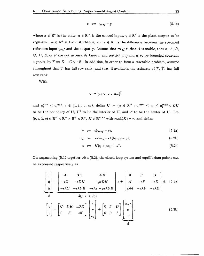
5.1. Constrained Self-Tuning Proportional-1ntegra.l Control 95
where x E Rn is the state, u E Wm is the control input. y E Rr is the plant output to be
regulated, w E Wq is the disturbance, and e E Rr is the daerence between the specified
reference input y,,f and the output y. Assume that rn 2 r , that A is stable? that n. A. B.
Cl D, E, or F are not necessarily known, and restrict gr.! and w to be bounded constant
signals; let T := D - CA-' B. In addition. in order to form a tractable problem? assume
throughout that 7 has full row rank, and that. if available. the estimate of 7. T. has full
row rank.
With
and uyin < u:axT i E {1'2.. . . ? m}. define U := { u E Rm : UT'" 5 Ui 5 ilyG}. aU to be the boundary of U, UO to be the interior of U. and uC to be the center of U. Let
(b , É, A, p) E Bi x R' x Rf x K E W m X r with rank(K) = r. and define
On augmenting (5.1) together with (5.2)? the closed loop systern and equilibrium points can
be expressed respect ively as
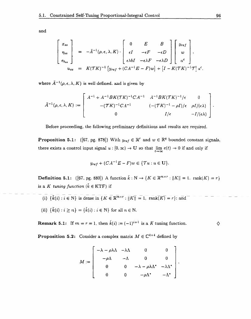
5.1. Constrained Self-Tuning Proportional-Integral Control 96
and
where A-' (p' E: A' K) is well defined. and is given by
A-' (p , E: A? K) :=
Before proceeding, the following preliminary definitions and results are required.
Proposition 5.1: ([67, pg. 8781) With y r e j E 8' and w E Wq bounded constant signais.
there eas ts a control input signal u : [O. x) + U so that lim e f t ) + O if and only if t - a
Definition 5.1: ( [67 . pg. 8801) X function ri. : N + { K E X m x r : il KI] = 1. rank(K) = r )
is a K tuning fvnction (k E KTF) if
Remark 5.1: If rn = r = l, then k ( i ) := (-l)'+' is a K tuning function.
Proposition 5.2: Consider a cornplex matrix M E cdX'' defined by
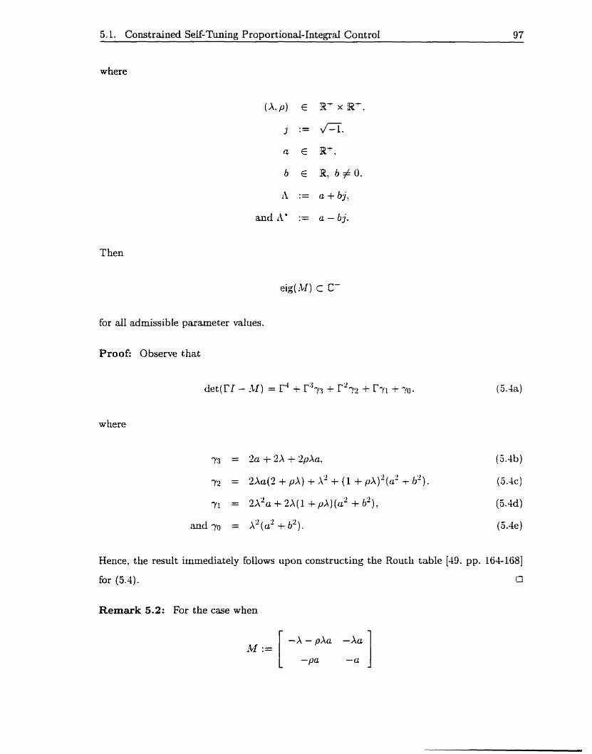
5.1. Constrained SeE-Tuning Proportional-Integrai Control 97
w here
and A* := a - bj.
for d l admissible parameter values.
Proof: Observe that
w here
Hence' the result irnmediately follows upon constructing the Routli table [dg. pp. 164-1681
for (5.4). (7
Remark 5.2: For the case when

5.1. Constrained Self-Tuning Proportional-Integrd Control 98
with (a. X?p) E P' x R' x Rt. it immediately follows that
eig(M) C C-
det (r I - hl) = r2 - ï trace(M) + det(M).
Furthermore. since
(a t X + ,da)' - 4aX = ( A - a)' + 2a2Xp + 2 a ~ ' ~ + a"'$,
and hence
O < (a + X i ,da)' - 4aX < ( a i X + p ~ a ) ' .
it therefore follows that
Lemma 5.1 : With (A. p ) E R' x B'. and eig(-TK) C 'CA. T K E Wr". çonsider the
matrix M E R' '~ '~ giwn by
for ail admissible paramet er values.
Proof: Let
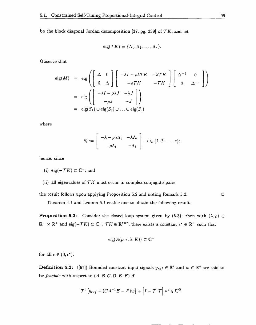
5.1. Constrained SeIf-Tuning Proport ional-Integral Control 99
be the block diagonal Jordan decomposition [37. pg. 3391 of TK. and let
e ig(7K) = :17, . . . , Ar).
Observe that
w here
hence, since
( i) eig(-TK) c C-: and
(ii) d l eigenvalues of TK must occur in coniplex conjugate pairs
the result follows upon applying Proposition 3.2 and noting Reuiark 5.2.
Theorem 4.1 and Lemma 5.1 euable one to obtain the following result.
Proposition 5.3 : Consider the closed Ioop system given by (5.3) : then with (A. p) E
IR+ x Etf and eig(-TK) C T K E RrXr . there exists a constant E' E P' such thst
for al1 E E (O, C).
Definition 5.2 : ([67]) Bounded constant input signals g , ,~ E Rr and w 6 R'l are said to
be feasible with respect to ( A , B. C, D. E. F) if
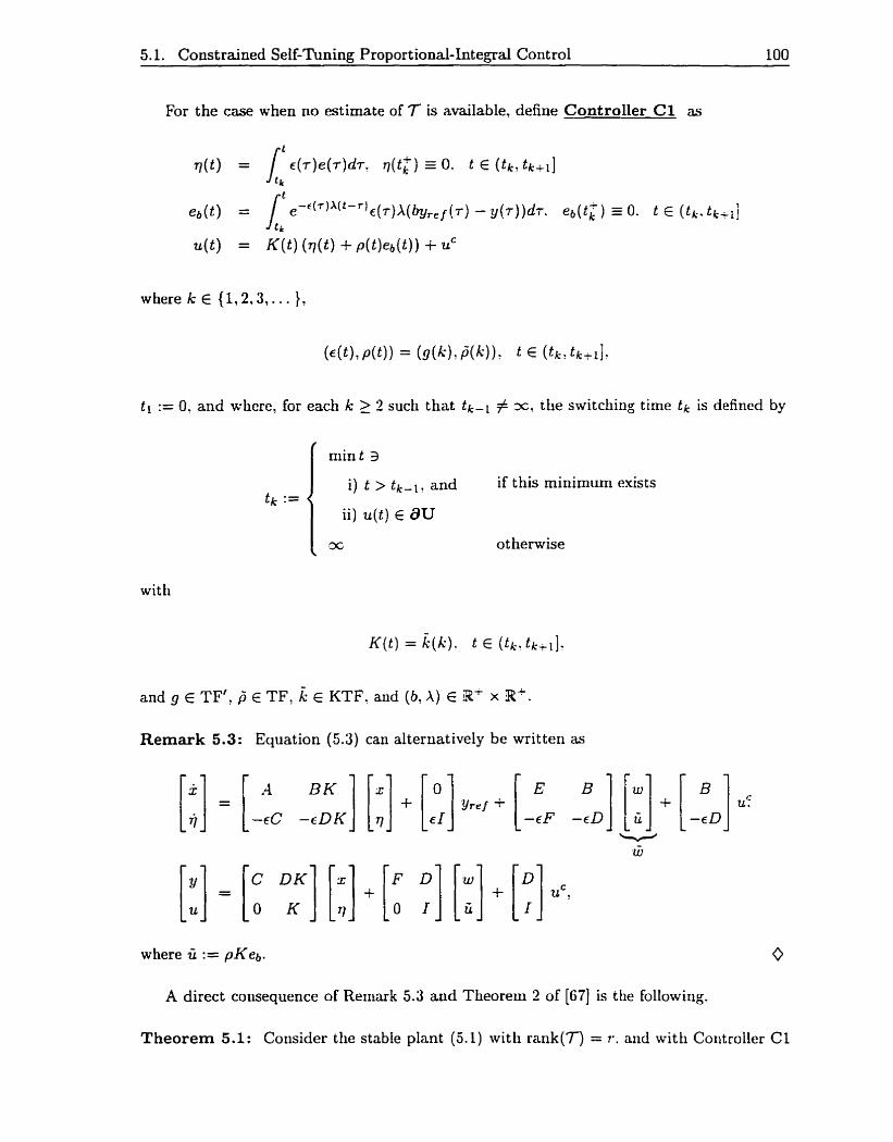
5.1. Constrained Self-Tuning Proportional-Integral Control 100
For the case when no estimate of 7 is available, define Controller Cl as
where k E ( l , Z , 3 , . . . ),
t l := 0, and where, for each k 2 2 such that t k - l # X, the switching time t k is defined by
i) t > t k - i , and if this minimum exists t k :=
ii) u( t ) E dU
I= O t herwise
wit h
and g E TF', P E TF, k. E KTF, and (b. A ) E Ri x R'.
Remark 5.3: Equation (5.3) can alteruatively be written as
where Û := pKeb. 0
A direct coiisequence of Reiriark 5.3 and Theoreni 2 of [67] is the following.
Theorem 5.1: Corisider the stable plant (5.1) with rank('T) = r. and with Coritroller C l
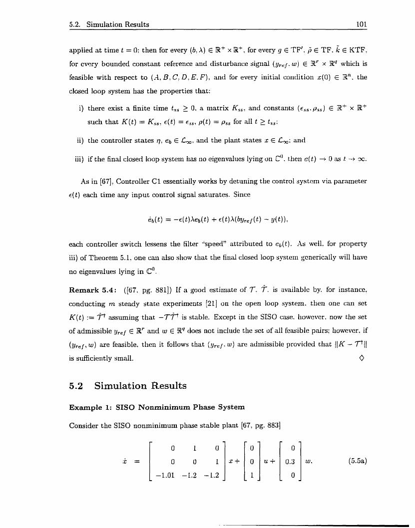
5.2. Simulation Results 101
applied at time t = 0: then for every (6: A ) E IIPt x Pt. for every g E TF'. 5 E TF. & E KTF.
for eviry bounded constant reference and disturbance signal (yreI. w ) E 3' x R(/ wtiich is
feasible with respect to (-4: B. C. D. E. F). and for evcry initial coiidition x(0) E Rn. the
closed loop system has the properties that:
i) there exist a finite time t,, 2 0. a matrix K,,. and constants (clS. p r s ) E $2- x Ef
such that K( t ) = Kss: ~ ( t ) = es,! p ( t ) = pss for al1 t 3 t,,:
ii) the controller states q! eb E L,. and the plant states z f Lm: and
iii) if the final closed loop systern lias rio cigenvaliics lying or1 .fO. tlien e ( t ) i D as t -+ x.
As in [67], Controller Cl essentially works by detuiiing tlie control systeni via parameter
~ ( t ) each time any input control signal saturates. Since
each controler switch lessens the filter -'speed" attributed to e b ( t ) . As weIlt for property
iii) of Theorem 5.1. one can d s o show that the final closed loop system gcnericnlly will have
no eigenvalues lying in CO.
Remark 5.4: ([ü7. pg. 8811) If a good estimate of 7. T. is availablc by. for instance,
conducting rn steady state experiments [21] on the open loop system. then one can set
K ( t ) := ? assuming that -7-fl is stable. Except in the SISO case. Iiowcvcr. now the set
of admissible gr,/ E Wr and w E g4 does not include tlie set of al1 feasible pairs: however. if
(%, j , w ) are feasible. tlien it follows that (yreI. w ) are admissible provided tliat III< - ( 1
5.2 Simulation Results
Example 1: SISO Nonminimum Phase System
Consider the SISO nonminimum phase stable plant [67! pg. 8831
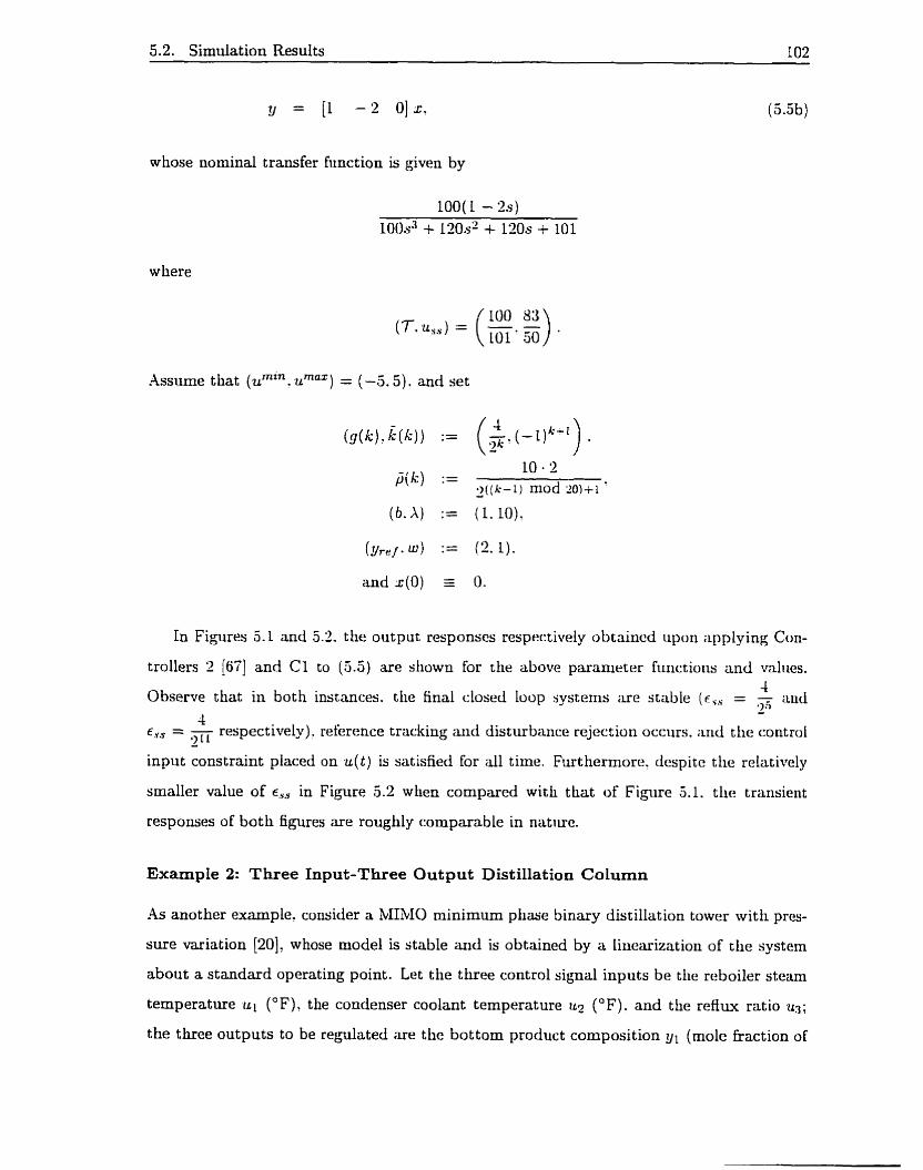
5.2. Simulation Results 102
whose nominal transfer function is aven by
where
Assume that (umfn. umm) = ( -5 .5) . and set
( y . w ) := (2.1) .
and x ( 0 ) O.
In Figures 3.1 and 5.2. the output responses respectively obtaincd iipcin applying Con-
trollers 2 [67] and C l to ( 5 . 5 ) are sliown for the above paranieter fiiiictiotis and values. 4
Observe that in both instances. the final closed loop systenis are stabie (E,, = - and '> .5 - il
e,, = ;iTT respectively). reference tracking aiid disturbance rejection occiirs. ;md the control - input constraint pIaced on ~ ( t ) is satisfied for d l time. Furtherrnore. despite the relatively
smaller value of E,, in Figure 5.2 when compared with that of Figure 5.1. tlie transient
responses of both figures are roughly comparable in nature.
ExampIe 2: Three Input-Three Output Distillation Column
-4s another example. consider a MIM0 minimum phase binary distillation tower with pres-
sure variation [20]. whose mode1 is stable and is obtained by a Iiueariïation of the system
about a standard operating point. Let tlie t h e e control s i p a l inputs be tlic rcboiler s t e m
temperature ui ( O F ) , the condenser coolant temperature uz ( O F ) . and the refiux ratio un;
the three outputs to be rebgdated are the bottom product composition y1 (mole Baction of
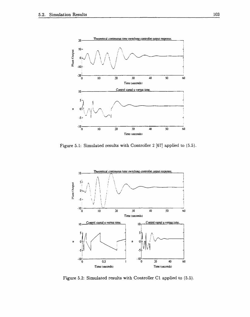
5.2. Simulation Results 103
IO, Thromticai continuous rime switching controller outpur mponse. 1 ,
Timr (seconds)
IO r Conuol stem1 u versus rime. (
Figure 5.1: Simulated results with Controller 2 1671 applied to ( 5 . 5 ) .
IO i Theore!ic;il continuous urne swttchine rontroller ciuipur rcsponse.
A
Tirnc t seconds)
'0; Conml simal u v m rime. Conml siend u versus rime.
'O'
Figure 5.2: Simulated results with Controller CI applied to (5.3).
5.2. Simulation Results 104
the more volatile component in liquid phase). the top product composition (mole fraction
of the more volatile component in Liquid phase). and the pressure 93 (atmosphere) [67, pg.
8843. With primary disturbance input w (mole Eraction of the more volatile component in
Iiquid phase) âssociated with changes in the input feed composition stream of the system.
restrict
and assume. after using the methods outlined in [21]. that the following estimate of 7 to
two significant digits is available:
Now with system matrices (A. B, C. D. E. F) given in Section B.4.
K( t ) := ? (see Remark 5.4).
(6. A ) := (2. LOO).
and x(0) O.
the results shown in Figures 5.3 and 5.4 are respectively obtained upon applying Controller
2 1671 and Controller C l to the distillation tower. In these figures. y ( t ) and ui ( t ) . y ( t )
and u2( t ) , and y3 ( t ) and un(t) are represented as solid, dashed. and dCuh-dot ted lines.
Observe that in this instance, the transient response shown in Figure 5.4 is discernibly
improved over that shown in Figure 5.3. In addition. in both of these cases. the final 0.5 0.5
closed loop systems are once again stable ( c , , = - and c,, = - respe~tiveiy)~ reference 27 35
tracking and disturbance rejection occurs. and the control input constraint imposed on u(t)
5.2. Simulation Results 105
is successfully maintained for al1 time.
Example 3: Four Input-Four Output lblulti-Zone Building Control
As a final example, consider the ILIIMO minimum phase part iaI decentralized teruperat ure
control problem of a multi-zone building whose stable mode1 was given earlier in (4.11). Let
g ( k ) :=
p f q :=
( b J ) :=
Y,&) :=
&Tm, (t) :=
and x(0) =
and restrict
Upon using these values and on applying Controllers 2 (671 and C l respectively to (4.11).
the output results shown in Fioves 5.5 and 5.6 are obtained, where y l ( t ) and ur(L). y2(t)
and u2(t), y3(t) and u3(t) , and y4 ( t ) and u l ( t ) are represented as solid. dashed. da&-dot tedt 10
and dotted Iines. Again, as eupected, the final closed loop systems are stable (E,, = in d
bot h instarices) , reference tracking and dist urbance rejection occurs, and the control input
constraint imposed on u(t ) is successfuily maintained for al1 time.

5.2. Simulation Resdts 106
Theoretical ccntinuous time switchine controlier output nrponse. 0.7 1 t
I l . i
= O J t - . , 1
C - . .
JJ - _ _ - - , . .---- . , . --- . . . . . - - - . .
1 - -- - . . - 1 . .
. . I I
l
-0.7 1 O 0.5 I 1.5 2 2.5 3 3.5 J 4.5 5
Time (seconds l 1 lo4
Coniml siend u vernis tirne. 2 , Cunuol s i e d u versus rime. 2 [ I t
, . . , . . . , . . . . . .. . .-. , , , ' < . .,. .. . .--
ii . , - ..-..--..-.---.-.-A . . . . . 1 ,, . . -. : .. : . -. . -- -1" l
1
-7 -0 500 iooo O 5
Timr (seconds) Tirne (seconds) s IOJ
Figure 5.3: Simulated resdts with Controller 2 [67] applied to a distillation tower.
O. 1 l-t~eoretical çonunuous rime switchinr conuoller output rcspunsc.
Conrml siend u vmus tirne. 2 Contml siend u vcnus rime. 11 I l
Figure 5.4: Simuiated resdts with Controuer C l applied to ü distillation tower.
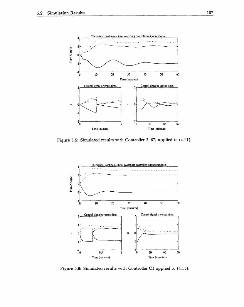
5.2. Simulation Results 107
Theoreticd cononuous u n e swilching connolla output response- . . . 7 I
O 10 20 30 JO 50 Ml
Time (minutes)
Figure 5.5: Simulated results with Controller 2 [67] applied to (4.1 1 ) .
Conuol signal u venus rime. 2 - Convol s i e d u versus time. 2
J : Thcoreiicai conunuous lime switchine conuoller output responsr. _ . - . _ _ 1
-J O IO 20 30 JO 50 60
Timc (minutes)
1
Conuol sienal u venus time. 2,
. - _ - _ . . . 3
-7 -2 -0 5 O 70 JO 60
Time (minutes) Time (mrnuces)
- _ - . 1
Canuol si na1 u venus rime. 2i
- . .
Timr (minutes) Time (minutes)
Figure 5.6: Simulated results with Controller C l applied to (4.1 1 ) .
Chapter 6
Adaptive Tracking of LTI MIMO
Systems
Using the metliods and results presented in Chapter 3: we consider now the finite dimen-
sional strictly proper MIMO adaptive tracking problem for the general class of reference and
disturbance signals wliose behaviour can be described by a Iinear cornbinatiori of botinded
piecewise continuous sinusoidal and polynomial functions. Ouce again. by monitoriiig plant
output y ( t ) and/or error signal e ( t ) the emphasis will be to provide a robust controller
which is insensitive to bounded piecewise continuou disturbances w ( t ) and whicli attempts
to provide au acceptable transient resporise. Initial simulation studies usirig t hese new
controllers tend to indicate that such desirable improvernents in the tuning response usu-
ally can be achieved rvtien compared with. for instance. the outputs obtained usirig the
computationally more intensive algorithms presented in 1591 and (661.
6.1 Preliminary Definitions and Results
Similar to Section 3.2, consider the finite dimensional strictly proper (stabilizable and de-
tectable) MIMO LTI system given by
x = -42 +Bu+ Ew,
y = Cz+ Fw,
e = Y r e j - Y
( 6 . l a )
(6.1 b)
(6. l c )
6.1. Preliminary Definitions and Resuits 109
where x E Rn is the state? u E Rm is the control input, y E Rr is the plant output to be
regulated, w E Rq is the disturbance, and e E Pr is the difference between the specified
reference input y,,~ and the output y. In addition? assume that n. -4. B. C. E. or F are
no t necessarily known. P
Let a(s ) := C aisL with p E M and np := 1. and let the roots of a ( s ) lie in C+ U CO: as r=O
weU, restrict
The control objective in this chapter will be to stabilize the system given by (6.l j such that
asymptotic reference tracking and disturbance rejection occurs for the class of yref(t) and
w(t ) defined by (6.2). Thus, in order to form a tractable problem [27]. assume too t hat
(i) m 2 r: and
(ii) the transmission zeros of (C. -4. B' O ) do not coincide with the zeros of a(s ) .
To form the servocompensator. consider the situation where matrices .i E RPXP and
B E RP are chosen so that det(s I - A) = ~ ( s ) and (.A. B) is controllable. Usirig [-71. defirie
.A8 := block diagonal (A.. . . . A) E RPrxPr .
B. := block diagorial (B.. . . . fi) E i lprxr .
and let the servocompensator < be given by
Combining plant (6.1) together with servocompensator (6.3): the augmented system can
therefore be written as
6.1. Preliminarv Definitions and Results 110
w here
Lemma 6.1: ([-SI) Given the plant (fi 1). the servocompensator (6 .3)- and the augnented
sys tem
then (A. B) is stabilizable and (G. -4) is detectable.
Due to the structure of the constructed servocompensator E , uny LTI controller wliich
stabilizes (6.4) will provide asymptotic error re ylation and dis turbance rejection [27].
Therefore, using the results given in Lemma 6.1. let the adaptive stabilizing controller
for (6.4) be of the form
6.1. Preliminary Definitions and Results 111
In addition, note that upon applying controller (6.5) to system (6.4). there always exists a
gi 5 n such that the final closed loop system is stable.
(i) {h(i) : i E W} is dense in for 6xed values ofgi E NU{O}. p E .lu{O};
and
(ii) for h(i) := 1 :: J p ~ . r - ~ r - g , ) ,
for constants ( r l : TV) E $3- x Sf.
Proposition 6.1: Given gi E N U (O). p E N u {O). there exists a h E GCTF.
Definition 6.2: Given that o! E NU { O } is a lower bound and that -y E .I u {O} is an
upper bourid on gi such that CI 5 gi < y with a < 7. a function h : M i ~ ( ' ~ - " ) ~ ~ - ~ ~ ~ g ~ )
is a modified yenerul controiier tuning Junction (h E GCTF') if. with (g,+ - gi) E {O. l}.
gi := cr? h(i) := Ri, and p E NU {O}. the following properties hold:
(iii) for h( i ) := 14 , - ~ ( - - g , ~ ~ ~ r + p r - g , ) .
for constants (rl, n) E R+ x R+.
Proposition 6.2: There exists a h E GCTF'.
Using the adaptive stabilization resuits of Chapter 3, the following results are obtaiued.
6.2. Using a Known Value of the Compensator Order 112
6.2 Using a Known Value of the Compensator Order
For the case whcn it is known that compensator (6.5) will stabilize the augrnented system
(6.4) with gi = 1 , 1 E N U {O}, using some appropriate clioice of controller matrices Gi, Hi,
Ki, Li, define Controller Tl as
where k E (1: 2: 3 , . . . }: h E GCTF.
t l := 0, and where, for each k 2 2 such that tk-1 # ccl the switching time tr; is defined by
I min t 3
if ttiis rniiiiniurri exists
ot herwise
with f E S2BF. Label Assumption T l to be
i ) IW) 1[ < f (1); and
Theorem 6. l: Consider the systern given by (6. l), and assume t h tliere exists a solut ion
to the robust servomechariism probiern for the class of reference and disturbarice signals
defined by (6.2); then with the corresponding servocompensator (6.3) implernented, and
with Controller T l applied at time t = 0, for every f E SSBF and h E GCTF, for every
bounded reference and disturbance signal of the form given by (6.2), and for every initial
condition [x(o)* ~ ( 0 ) ~ q ( ~ ) T ] T for which Assumption Tl holds, the closed loop systeni lias
the properties that:

6.3. Using no Known Value of the Compensator Order 113
ii) the controller states <, 77 L,, and the plant states x E L,; and
iii) for almost al1 controller parameters (G1 H, K, L), the final eigenvalues of the closed
loop system will lie in C.
6.3 Using no Known Value of the Compensator Order
For the case when it is known that compensator (6.5) will stabilize the augrnented system
(6.4) with gi = 1 using some a 5 1 5 y with a, y E N U {O): cr < y' and using some
appropriate choice of controller parameters Gi, H*, Ki , Li: label Controller Tl' to be
Controller Tl, but with h E GCTF'.
Theorem 6.2: Consider the system given by (6.1) , and assume that t here exists a solution
to the robust servomeclianism problem for the class of reference and disturbancc signals
defined by (6.2): t hen wit h the corresponding servocomperisator (6.3) implemented. and
with Controller Tl' applied a t time t = 0. for every f E S2BF and h E GCTF'. for every
bounded reference and disturbance signal of the form given by (6.2): and for every initial
condition [x(0)= ~ ( 0 ) ~ q ( ~ ) T ] T for which Assumption Tl Iiolds. the closed loop system has
the properties that:
ii) the controller states c , I) E Lm? and the plant states x E L,: and
iii) for almost al1 controller parameters (G, H , K, L). the final eigenvalues of the closed
loop system will lie in @-.
If A is stable and if a ( s ) = s, then the controllers proposed in Chapter 4 of this t hesis
can be used to achieve asymptotic reference tracking and disturbance rejection for t his
particular class of signals. As well, upon filtering Y ( t ) as
6.3. Usine: no Known Value of the Compensator Order 114
and upon making corresponding changes in t fie assumpt ion and controller defini t ions (e.g.
see Theorem 2.2 and Rernark 3.5), Theorems 6.1 and 6.2 will also work for those refer-
ence and disturbance signals whose behaviour can be described by a linear combination of
bounded piecewise continuous sinusoidal and polynomial functions. Furtherniore, the com-
ments given in Remark 3.4 are equally valid for for Theorems 6.1 and 6.2. In this instance,
by using more system information, and tience, by reducing the parameter space scarch for
a stabilizirig h ( i ) , one would therefore also expect an improved output transient response.
Remark 6.1: ([21]) If A is stable in (6.1) and the roots of a ( s ) lie in @O. tlieo there exists
a gain K E IRmxpr so that  + B[O K]C is stable. Hence? if plant (6.1) Iias an l'th-order
s tabih ing compensator, then the augmerited system given by (6.4) does as well. 0
One can dso combine plant (6.1) together with servoconipensator (6.3) to form the
augrnented system
A* z* B* E* fi*
where (A*, B*) is stabilizable and (Cu. A') is detectable. Hence. Controllers T l and Tl'
will also work iising the switching mechanism defined by
niin t 3
i) t > t k - ~ , and t,, :=
ii) llE(t)ll = f (k - 1)
00
if this minimum exists
O t herwise,
where
6.4. Simulation ResuIts L 15
assuming that lle(0)11 < f(1) and 11<(0)11 < f (1) also hold at time t = 0.
6.4 Simulation Resuits
Example 1: SISO Unstable Minimum Phase Plant
Consider the (controllable and observable) unstable minimum phase SISO plant [66. pg. 571
with open loop eigenvalues of -2 and 1. and assume that there exists a solution to the
robust servomechanism problem for constant references and constant disturbances. Let
.y,&) := 10' w ( t ) := 1.
3.5k. 1 5 k 5 1 5 f (k) :=
30(k - 15)' exp((k: - 15)". k > 15.
and set al1 controller-plant initial conditions to be equal to zero at time t = O. Since
rn = r = 1 and a ( s ) = .S. a choice of (A*. B * ) = (0.1) yields an appropriate corresponding
servocompensator ( for the particular class of reference and disturbance signals chosen.
Assume that the given plant (6.6) is unknouin. but that it is known that there exists
a zero'th-order stabilizing compensator for the open loup system. In addition. using the
comments given in Remark 6.1 and the results given in [21]. it sutnces to search for a
stabilizing feedbadc matrix Li in the set P x [- 1.11; hence, define h( i ) as
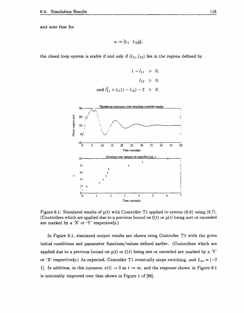
6.4. Simulation Results 116
and note that for
the closed loop system is stable if and only if (Z11?lL2) lies in the regions defined by
1 - l L L > 0:
LI, > 0.
and 1:1 + l i i ( l - i l2) - 2 > O.
30, Theoretical contmuous rime swirchinq contmllcr reniirs. 1
1 - s 10; h t
10. Switchine rrmr instuits of conuollrr k t - v . \
l
Figure 6.1: Sirnulated results of g ( t ) with Coutroller Tl applied to systeni (6.6) using (6.7). (Controllers which are applied due to a previous bound ou < ( t ) or y ( t ) being met or exceeded are marked by a 'X' or -Y7 respectively.)
In Figure 6.1, simulated output results are shown using Controller T l with the given
initial condit ions and parameter functions/values defined earlier. (Controllers which are
applied due to a previous bound on y ( t ) or f ( t ) being met or exceeded are marked by a 'Y?
or 'X' respectively.) As expected. Controller T l eveutually stops switching, and L,, = (-2
1). In addition, i11 this instance, e ( t ) -+ O as t -+ m. and the respouse shown in Figure 6.1
is noticeably improved over that shown in Figure 1 of (661.

6.4. Simulation Results 117
Example 2: SIS0 Stable Nonminimum Phase Plant
As a second example, consider the (controllable and observable) stable nonminimum phase
SIS0 plant 1501
(with open loop poles at -1 and zeros at 0.5) whem it is assumed that (6.8) is known only
to be stable' and that a solution to the robust servomeclianism problem exists for coristant
references and constant disturbances. Using the results given in Rcrnark 6.1 and [?Il. define
h( i ) as follows:
With
the closed loop system is stable if and only if
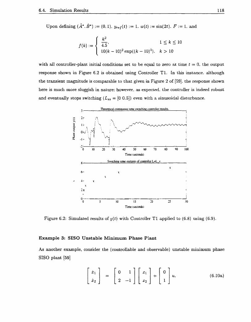
6.4. Simulation Results 118
- Upon defining (A*. B*) := (0.1). gref(t) := 1. w ( t ) := sin(2t). F := 1. and
with al1 controller-plant initial conditions set to be equal to zero at time t = O. the output
response shown in Figure 6.2 is obtained using Controller Tl. In this instance. although
the transient magnitude is comparable to that given in Figure 2 of [59]. the response shown
here is much more sluggish in nature: however. as expected. the controller is indeed robust
and eventually stops switching (L,, = [O 0.51) even with a sinusoidal disturbance.
3 Theoretlrril continuou time switchinc rontmller rcnilrs. I
-0 10 20 30 Ul 50 60 70 $0 40 100
Time (seconds)
8 * Switchine urne instants of controilcr L=L-V.
O 5 10 15 10 '5 3 0
Time iswonds)
Figure 6.2: Simulated results of y ( t ) with Controller TI applied to (6.8) usiag (6.9) .
Example 3: SISO Unstable Minimum Phase Plant
As anot her example, consider the (controllable and observable) unstable minimum phase
SISO plant [59]
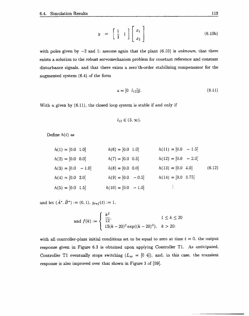
6.4. Simulation Results 119
with poles given by -2 and 1: assume again that the plant (6.10) is i~nknouin. t hat there
exists a solution to the robust servomechanism problem for constant reference and constant
disturbance signals. and t hat t here elusts a zero'th-order stabilizing compensator for the
augmented system (6.4) of the forni
With u given by (6.1 l ) , the closed loop system is stable if and o d y if
E (3. x).
and let (A*. B*) := (0,1), grel(t) := 1.
1 g i Y g o and f(k) :-
15(k - 20)' exp ( (k - 20)"). k > 20:
with d controller-plant initial conditions set to be equal to zero at time t = 0. the output
response given in Figure 6.3 is obtained upon applying Controller T l . As anticipated.
Controller T l eventudy stops switching (L,, = [O 41): and, in this case. the transient
response is also improved over that shown in Figure 3 of [59].

6.4. Simulation Results 120
Timr ( sesonds )
Figure 6.3: Simulated results of y ( t ) with Controller TL applied to (6.10) usirig (6.12).
Example 4: MIS0 Unstable Minimum Phase Plant
Finaily, consider once again the (stabilizable and observable) unstable minimum phase
MIS0 p l u t [62. pg. 6051 given in (3.8). Assume that the plant (3.8) is unknoiun. that there
exists a solution to the robust servomechanism problem for coristant reference and constant
dist iirbance sipals. and t hat t here exists a zero't h order s tabilizing cornpeusatoc for the
augrnented system (6.4) of the form
One can verify that wit h u given by (6.13). the closed loop system is stable if and onIy if
and (0.1 +O.llll +112+4122)(-2-11L l L 2 > 0.
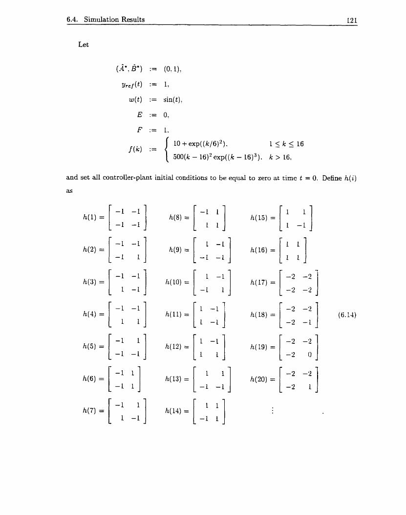
6.4. Simulation Results 121
Let
(A*' B') := (O. l )?
~ l r e f ( t ) := 1:
w ( t ) := sin@),
E := 0,
F := 1.
and set al1 controller-plant initial conditions to be equal to zero at time t = O. Define h(i)
as

6.4. Simulation Results 122
One can veri& t hat for the given listed values of h(.i),
h(2) : h(10). and h(20)
form stable closed hop systems.
In Figure 6.4. output results are shown using Controller TI with the prcvioiisly defined
parameters and funct ions. Xgain. as anticipated. the controller eventudly stops switching?
wit h
and the controller is indeed robust even with a persistent. sinusoidd disturbance. For com-
parison. using h( i ) defined as

6.4. Simulation Results 123
the larger output transient response given in Figure 6.5 is obtained. and
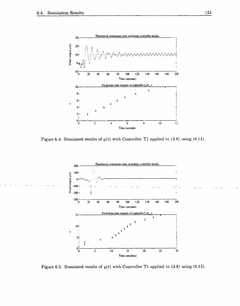
6.4- Simulation Results 124
Thromid continuous tirne switchine contmllrr mula. 1
Timr 1 seconds)
Figure 6.4: Simulated results of y(t) with Controller T l applied to ( 3 . 8 ) iising (6.11).
100 Thr<lrrncJ continuaus tirne swrtching i o n m l k r wulrs.
Timr (seconds)
Figure 6.5: Simulated results of y(t) with Coutroller TL applied to (3.8) iising (6.15)-
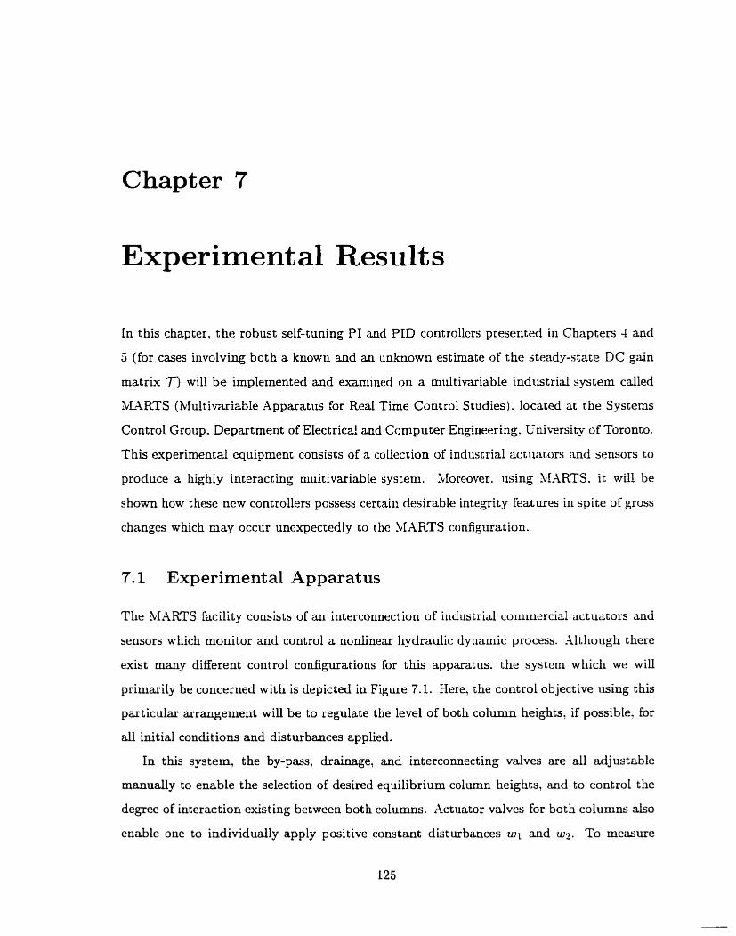
Chapter 7
Experiment al Result s
In t his chapter. the robust self-tuning PI and PID controllers presented iri Chapters 4 and
5 (for cases involving both a known and an unknown estimate of the steady-state DC gain
m a t r ~ ~ T) will be implemented and examined on a multivariable industrial system cailed
LUIARTS (Multivariable Apparatus for Red Time Control S tudies). located at the Systems
Control Group. Department of Electrica! and Computer Engineering. University of Toronto.
This experimental equipment cousists of a collection of industrial ac t iiators rmd sensors to
produce a highly interacting multivariable system. hforeover. using MARTS. it wil! be
shown how these new controllers possess certain desirable integrity féatures in spite of goss
changes which may occur unexpectedfy to the ,LIARTS configuration.
7.1 Experimental Apparatus
The MARTS facility comists of an intercomect ion of industrial conimercial actuators and
sensors which monitor and control a nonlinex hydraulic dynamic process. Although there
exist many different control configurations for this apparatus. the system which we will
primarily be concerned with is depicted in Figure 7.1. Here, the control objective using this
particular arrangement will be to regulate the level of both column heights, if possible, for
al1 initial conditions and disturbances applied.
In t his system, the by-pass, drainage, and interconnecting vaives are al1 adj ustable
rnanually to enable the selection of desired equilibrium column heights, and to control the
degree of interaction existing between both columns. Xctuator valves for both columns abo
enable one to individudly apply positive constant disturbances wi and .wz. To mesure

7.1. Experimental Apparat us 126
By-pass Valves ControI Valves,
~ c t u a t o r Valve (to produce
disturbances)
Output 91 l Column 1 i Column 2
L (to produce
dis t ur bances)
7 Tub Valves -
Figure 7.1: Schematic diagram of one possible SLARTS arrangement (not to scale).
both column heights (through the use of a curent-pressure transdiicer) and to control the
actuator and control valves (by using a current-pneumatic actuator). a Texas Instruments
(TM W O / 101/bIX-1) real time digital computer using the PDOS operating system with an
addit iond 12 bit analog-digital (-A/D) and digital-analog (D / -1) board (not s hown) is used.
Valid inputs u to the control valves are t herefore restrictcd numerically CO the intervai
O (shut) 5 u 5 4095 (fully open)!
while column height measurements h generalIy fali in the range (due to the sensors' cali-
bration) of
1200 (bottom) < h 5 4095 (top).
Physically, this later interval corresponds to a height range of about 1.3 meters. or. equiv-
alently, to approximately 0.4 mm. per digital division of resolution.
In Table 7.1, a listing of some of the va.rious major components of the LIARTS appa-

7.2. Linearized Model of MARTS 127
ratus is given. Note that as the interconnecting valve angle increases from O" to 45'. the
ry
Control valve transducsr 1 Foxboro E69P current-to-pneumatic valve posit ioner 1
By-pass vdve Interconnec t ion valve Pump Level sensor Control valve
Table 7.1: Summary of the major cornponents of MARTS.
Part Drainage valve
1/2 inch globe valve 1/2 inch bal1 valve Iwaki centrifuga1 pump (1/ 12 HP) Taylor 3400T Series pressure differential transmit ter Foxboro V4A 1/2 inch linear valve
plant becomes increasingly difficult to controII and that due to the valve transducers used,
bot h coutrol valves utilize a mechanical feedback Linkage to give an equilibriurn valve po-
sition that is proportional to t lie input current signalL. Additional informat ion concerning
the equipment used, the system startup procedure, as well as ottier possible experimental
configurations can be found in [22].
Since niariy commonly used controller synthesis design techniques need an accurate
representation of the actual plant, and since conventional adapt ive cont rollers still typically
require specific plant information (e.g, the order of a stabilizing controller. an upper boiind
on the order of the plant, the relative degree of the plant) in order to c a r a n t e e acceptable
controlIer performance, the variable structure of MXRTS preseuts an ideal situation for
one to implement and examine the robust self-tuuing PI and PID cotitrollers proposed iri
Chapters 4 and 5.
Descript ion 1/2 inch globe valve
7.2 Linearized Model of MARTS
In order to denionstrate the general difficuity and uncertainty ili obtainirig an accurate
mode1 representation of an unknown system. consider the interconnectioii structure of
MARTS shown in Figure 7.2.
Let i E {l ,2) , and define
ui := input to controi valve z,
'This occurs as opposed to using pneumôtic feedback to give an equilibrium output pressure that is proportional to the input current signal.
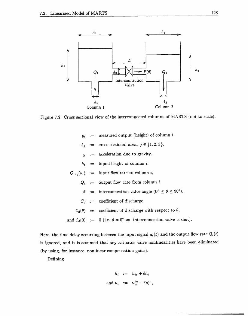
7.2. Linearized Mode1 of MARTS 128
m -4 1 .-h - - -
li-iterconnection
e
-A2 Column 2
Figure 7.2: Cross sectional view of the interconnected columns of !vIARTS (not to scale).
measured output (height ) of column i.
cross sectional area. j E { 1.2.3} .
acceleration due to gravity.
liquid Lieight in column i.
input flow rate to colunin i.
output flow rate from columri i.
interconnection vaIve angIe (O0 5 19 5 90').
coefficient of discharge.
coefficient of discharge with respect to 8.
O (i.e. 8 = 0° e interconnection valve is shut).
Here, the time delay occurring between the input signal ui ( t ) and the output flow rate Q i ( t )
is ignored, and it is assumed t hat any actuator valve nonlinearit ies have been eliminated
(by using, for instance, nonlinear compensation gains).
Defining

7.2. Linearized Mode1 of MARTS 129
where hi, and ui: are. respectively. tlie steady state lieigtit of aiid input to coliinin i and
control valve i! the following linearized niodel of MXRTS can be obtained for the case wfien
hls > h2s [l4]: [511:
w here
In (7.1), is the perturbed liquid level of column i (i E {1.2}). and (hli is the perturbed
input liquid flow rate froni control valve i entering coIumn i.
Remark 7.1 : .A similar derivation for the case when hl, < h2, yields t Lie sarrie basic
format for (7.1): with
being tlie only slight modification needed. In addition. for ttic case when hl, S i~? , arid
B # O". one can also show [ I I ] that tlie systern beliaves as a single colttmn apparatils obeying
the equations
where X := 6hi + Sh2: and where the (redistic) assumption is made tliat 0 := Pi % h.
Hence, (7.1) may be seeu to be equally valid under this partictilar condition. 0
Using the experimental apparat us with the interconnection valve angle B set at 30" : (Bi !
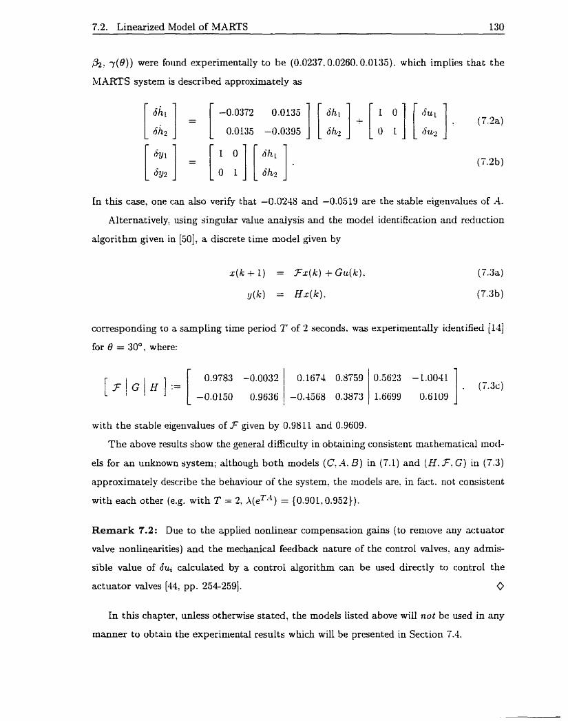
7.2. Linearized Mode1 of b1ARTS 130
,&? ~ ( 0 ) ) were found experimentally to be (0.0237.0.0260.0.0135). which implies that the
CVIARTS system is described approximately as
In this case, one can also verify that -0.0248 and -0.0519 are the stable eigenvalues of A.
Alternatively, using singular vdue analysis and the model identification and reduction
algorithm given in [50], a discrete îime model given by
( k ) = H.c(k) .
corresponding to a sampiing time period T of 2 seconds. w a
for 8 = 30". where:
experimentally identifid [Id]
with the stable eigenvalues of .? given by 0.98 11 and 0.9609.
The above results show the generai difficulty in obtaining consistent mathematical mod-
els for an unknown system: although both models (C. -4.8) in (7.1) and ( H . 3. G) in (7.3)
approximately describe the beliaviour of the system, the models are. in fact. not consistent
with each other (e.g. with T = 2, ~ ( e ~ - ' ) = {0.901,0.952)).
Remark 7.2: Due to the apphed nonlinear compensation gains (to remove any actuator
valve nonlinearities) and the mechanical feedback nature of the control valves, any adrnis-
sible value of dui calculated by a control algorithm can be used directly to control the
actuator valves [44, pp. 2542591. 0
In t his chapter, unless otherwise stated, the models listed above will nat be used in any
mamer to obtain the experimental results which will be presented in Section 7.4.
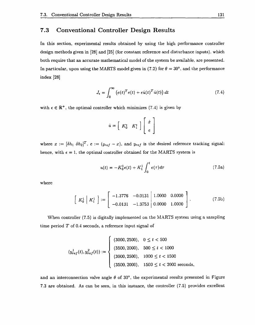
7.3. Conventional Controller Design Results 131
7.3 Conventional Controller Design Results
In this section, experimental results obtained by using the high performance controller
design met hods given in [28j and [25] (for constant reference and disturbance inputs). which
both require that an accurate mat hematical mode1 of the system be available, are presented.
In particular, upon using the MARTS mode1 given in (7.2) for 8 = 30°, and the performance
index [28]
wit h é E the optimal controller which minimizes (7.4) is given by
where x := [bhi 6h2IT, e := - r), and y, ,~ is the desired reference tracking signal:
hence, with E = 1. the optimal controller obtained for the MARTS system is
where
When controller (7.5) is digitally implerrrented on the MAARTS system usirig a sarnpling
time period T of 0.4 seconds, a refereuce input signal of
1 (3500,2000), 1500 5 t < 2000 seconds,
and an interconnection valve angle 0 of 30": the experimental results prese~ited in Figure
7.3 are obtairied. As can be seen, in this instance, the controller (7.5) provides excellent
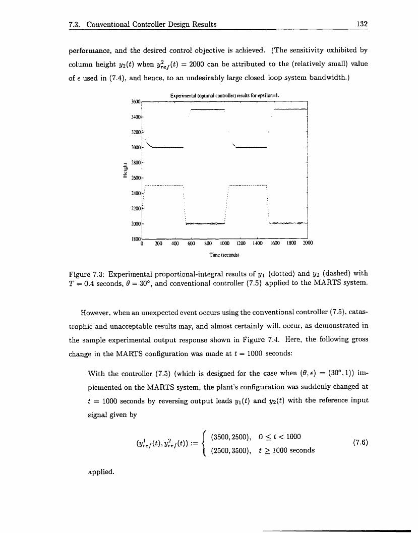
7.3. Conventional Controller Design Results 132
performance, and the desired control objective is achieved. (The sensitivity exhibited by
column height ~ ( t ) when g:ej(t) = 2000 can be attributed to the (relatively small) value
of E used in (7.4), and hence, to au undesirably Large closed loop system banrlwidth.)
Expenmental ( o p ù m l conuallrr) resuits for qsi lon=l. 3600 i
1 34001
Figure 7.3: Experimental proportional-integral results of y1 (dotted) and y2 (dashed) with T = 0.4 seconds, 0 = 30°, and conventional controller (7.5) applied to the MARTS system.
However, when an unexpected event occurs usiiig the conventional controller (7.5), catas-
trophic and unacceptable results may, and alniost certainly will. occur, as demonstrated in
the sample experimental output response shown in Figure 7.4. Here? tlie followiiig goss
change in the MARTS configuration was niade at t = 1000 seconds:
With the controller (7.5) (wliich is designed for the case when (O , 6) = (30°, 1)) im-
plemented on the MARTS system, the plant's configuration was suddenly clianged a t
t = 1000 seconds by reversing output leads y , ( t ) and y2(t) witli the reference input
signal given by
(3500,2500), O 5 t < 1000 (3;. j (t) 1 t ~ : ~ j ( t ) ) :=
(2500,3500), t 1 1000 seconds
applied.

7.3. Conventiond Controller Desim Results 133
Figure 7.4: Experimental proportional-integral results of y1 (dotted) aud y2 (dashed) with T = 0.4 seconds, 6 = 30°, and with the outputs reversed at t = 1000 seconds, showing failure of convent ional controller (7.5).
Figure 7.5: Experimental proportional-integrd results of y1 (dotted) and g2 (dashed) with T = 0.4 seconds, O = O", and with the outputs reversed a t t = 1000 seconds, showing failure of convent ional controller (7.5).

7.4. Switching Controller Output Results 134
As can be seen, in this situation, the closed loop system fails to track (7.6) for such a
severe codguration change: indeed, even with 8 = O". Figure 7.5 shows that a sirnilar
problem still occurs on applying controller (7.5) with T = 0.1 seconds to the MARTS
system. Unfortunately. such failures of this type r'if controller ;ire not unexpected. since
drastic changes in the plant have occurred at t = 1000 seconds.
It will now be shown that one class of the self-tuning robust servornechanism controllers
proposed previously does not have this limitation in the sense that these specified controllers
can readily adjust to severe plant contiguration changes'.
7.4 Switching Controller Output Results
As evidenced in Section 7.3. conventional controller (7.5) is unable to carry out its specified
mandate when gross structurai changes occur to the MARTS configuration. Hence. consider
the following definition of intelligent coutrol adopted from [23] and [17].
Definition 7.1 : An intelligent controller for a plant is a controller wliicli successfully
carries out its mandate for the plant's nominal operating conditions. as well as for any
unezpected (i.e. ,unplanned) events which may occur.
Mt hough Definition 7.1 is loose in the sense t hat the wording mi& not bc considered to
be well defined. the flavour of the definition is clear. For example. if one drs igns a controller
so that it successfuily controls the nominal plant -,4f" as well as when the plant is in some
failure mode .X'? Say. then the controller has the property that it displays certain integrity
leatures (which is very desirable). but the controller is not intelligent: the controller is
intelligent only if it successfully controls the plant. either in nominal mode or failure
mode .X'. in spite of the fact that failure mode 'K' was not unticipated in the design of the
controuer.
In this section, the self-tuning proportional-integral (PI) and proportional-integal-
derivat ive (PID) controllers presented earlier in Chapters 1 and 5 will be implemented
and exmined on the MARTS apparatus. Using almost no a priori system informat iono in
Sections 7.4.2: 7.4.3, and Appendix C, Controllers PID1' (Theorem 4.5) and Cl (Theorem
' ~ u e to the nature of the controllers considered, plant configuration chimges whicli maintain the assump- tions that eig(=l) C @- and rank(7) = r only will be considcred.
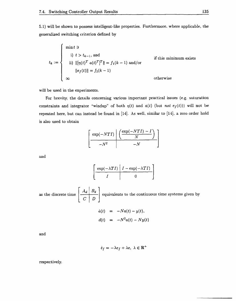
7.4. Switching Controller Output Results 135
5.1) will be shown to possess intelligent-like properties. Furthermore. where applicable, the
generalized switching crit erion defined by
i) t > tk-l$ and if t bis minimum exists
ii) I l [q~( t )~ a ( t ) T ] T ~ ~ = fI(k - 1) and/or
ot henvise
will be used in the experiments.
For brevity, the details concerning various important practical issues (e.g. saturation
constraints and integrator "windup" of both ~ ( t ) and a ( t ) (but not ef(t))) will not be
repeated here, but can instead be found in [14]. As well. similar to [l-l], a zero order hold
is also used to obtain
and
as the discrete time equivalerits to the continuous time systen~s giveri by
and
eI = -Xej + Xe, X E W+
respect ively.
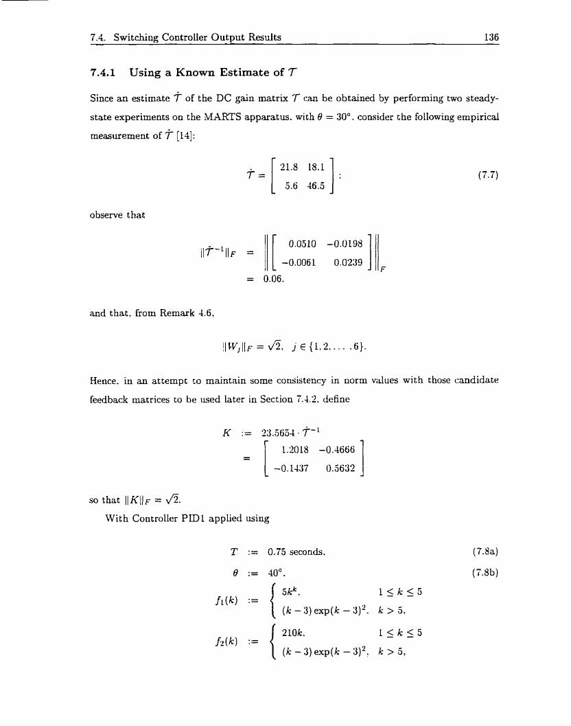
7.4. Switching Controller Output Results 136
7.4.1 Using a Known Estimate of 7
Since a n estimate T of the DC gain matrix 7 can be obtained by performing two steady-
state experiments on the KARTS apparatus. with 8 = 30". consider the following ernpirical
measurement of T [14]:
observe that
and that. from Remark 4.6?
Hence. in an attempt to maintain some consistency in norm values with those candidate
feedback matrices to be used later in Section 7.4.2. define
W i t h Controller PID 1 a p plied using
T := 0.75 seconds.
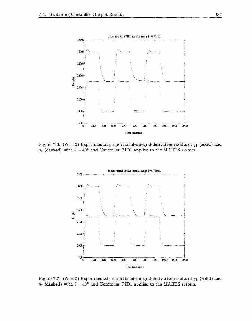
7.4. Switching Controller Output Results 137
Figure 7.6: ( N = 3) Experimental proport ional-integral-derivat ive results of y1 (solid) and g2 (dashed) with 6, = 40' and Controller PIDl applied to the MAARTS systern.
Figure 7.7: (N = 5) Experirnental proportionai-integrai-derimtive results of y1 (solid) and y:, (dashed) with 0 = 40° and Controller PID l applied to the MARTS systern.
7.4. Switching Controuer Output Results 138
(:3000.2500). 1200 5 t < 1500
(2500.2000). t 3 1500 seconds.
p := 20. (7.8d)
and X := 10. (7.8e)
the output responses shown in Figures 7.6 and 7.7 are obtained for the case when LV := 3
and N := 5 respectively. In both examples. q ( t ) is not reset to be eqiial to zero immediately
following any controller switch, and. as expected. the controller eventrially stops switching
(a total of three switches occurs in each figure). In addition, altliough the intercon~iection
valve angle 0 is now set to be equal to -10". tracking of the given rcference Iieights occiirs.
and the controller is indeed robust.
7.4.2 Using no Known Estimate of 7
In Figure 7.8. the output response obtained using Controller PIDI' and (7.8) witli
P(k) := 3 5 . (((k - 1) mod 6) + I), (7.90
and no a priori estimate of T is shown; in this instance, utilizing the cyclic switching
action summarized in Table 4.1 (with a ( t ) and e f ( t ) both additionally reset to be equal
7.4. Switching Controffer Output Results 139
to zero immediately following any controller switch), a total of 18 switches occurs within
approximately one minute. and tracking of ( 7 . 8 ~ ) once again is achieved. As in Figures 7.6
and 7.7. the sluggish behaviour which is apparent in yi(t) during the initial transition in
height from 3000 to 2500 can be attributed primarily to valve saturation constrainis.
For cornparison. in Figure 7.9, experimental results are presented using Controller PIDI'
and the identical system setup as given for Figure 7.8. but wit h output l a d s y l ( t ) and ?j2( t )
init ially reversed.
(h:,I ( t ) hLl ( t ) ) := (3000.2500). t 3 O.
and with positive constant disturbance w2 applied to column 2 a t time t = O. In tbis case.
there is a total of 23 switches. and tracking of (7.10) occurs after approximately 800 seconds.
Furthermore. from (7.7): these results are entirely consistent in the fact that for Figure 7.8.
wfiile for Figure 7.9:
As a final example, in Figure 7.10. output results for Controller PID1' are shown iising
(7.9) with
T := 0.75 seconds,
8 := 20':
( ( t ) ( t ) ) := (2500.2250). t 2 0.
p := 20.
X := 107
and wit h both output leads reversed after 1200 seconds. Once again. as anticipated, tracking
of the given reference heights occurs, and k,, = 24. Xlternatively. using (7.9) and (7.11)
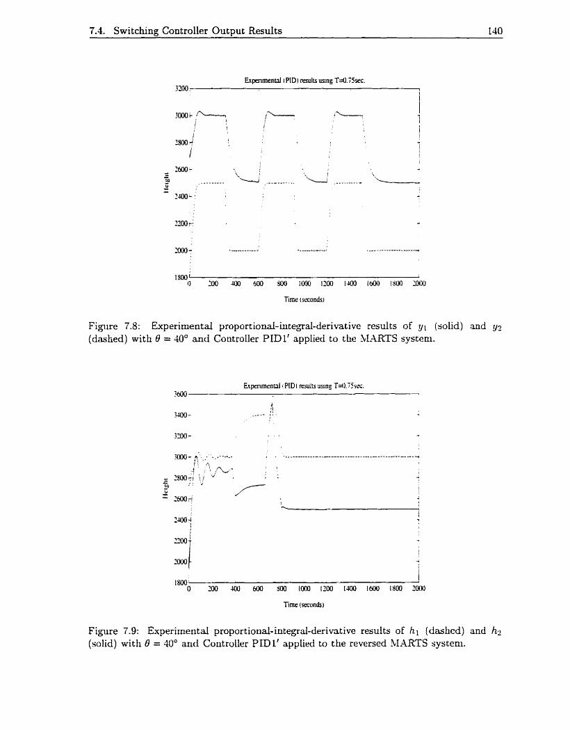
7.4. Swi tching Controller Output Results 140
Figure 7.5: Experimental proportional-integral-derivative results of 91 (solid) and y? (dashed) with 13 = 40" and Controller PIDl' appIied tu the MXRTS systeni.
1 LOO T
Figure 7.9: Experirnental proportional-integrai-derivative results of hl (dashed) and hl (solid) with 8 = 40' and Coritroller PID 1' applied to the reversed MARTS systeni.

7.4. Switching ControlIer Output Results 141
l 1 1
-*-- -1 ml-
Time (seconds)
Figure 7.10: Experimental proportional-integral-derivat ive rcsrilts of y 1 (solid) and y2
(dashed) with 6 = 30° and Controller PIDL' applied to the MARTS system.
Figure 7.11: Experimental proportional-integraI-derivative results of 91 (solid) and (dashed) with Controller PIDI' applied to the MARTS system.
7.4. Switching Controller Output Results 142
with no output lead reversa1 and
40'. O 5 t < 750 Q ( t ) :=
O". t 2 750 seconds.
the resuits shown in Figure 7.11 are obtained and k,, = 19.
Additional experimental results obtained ilpon applying Controller PID 1' to 41ARTS
are summarized in Appendix C.
7.4.3 Using ControlIer Cl
For a final set of experimental results, let
èb = -€Xeb + cX(b?~,. - y ) . (6. e . A) E B' x BT x R1.
On applying Controller C 1 (in order to eliminate any potent ial reset windup issues caused
by control signal saturation constraints) with no a prion estirnate of 7. and on using the
cyclic switching action for K ( t ) siinimarized in Table 4.1. together witli
g2(k) :=
8 :=
(6:X) :=
.- and ( ~ ~ e ~ ( t ) ~ ~ ~ t = ~ ( t ) ) * -
0.5 seconds.
10 $(k- 1 ) mod 6)+ 1 '
2 2 ( ( k - L) mod i-o)+i ' 30".

7.4. Switching Controller Output Results 143
the output results shown in Figures 7.12 and 7.13 are respectively obtained for &(k) :=
5 - g2(k) and P(k) := O. In both instacces. switching eventually ceases (k , , = 85 aad
kss = 61). and tracking of yref(t) occurs after approximately 500 seconds.
Alternatively. for the case when (7.12) is applied with Controikr CL using
(6.X) := (1.50):
( y ( ) ( t ) ) := (25OO.%OO).
and with output leads y ( t ) and yu ( t ) suddenly reversed at t = 1500 seconds. the respective
results shown in Figures 7.14 and 7.15 are obtained for p ( k ) := 0.05 . ga(k) cznd @(k) := 0.
Once again. switching eventually ceases (k,, = 66 and k,, = 72). and tracking of the given
reference inputs still occurs despite the unanticipated drastic plant changes w hich take
place at t = 1500 seconds. Moreover: in both of the situations presented here. Controller
C l does indeed successfuily result in a noticeably improved tuning transient response when
compared with that obtained by using Controller 2 given in [67].

7.4. Switching Controller Output Results 144
Figure 7.12: Experimental proportional-integral results of y1 (solid) and y:, (dashed) with 9 = 30" and Controller C l applied to the MARTS system.
Timr (seconds 1
Figure 7.13: Experimental integral results of y1 (solid) and y:! (daslied) with 8 = 30" and Controller 2 [67] applied to the MARTS system.
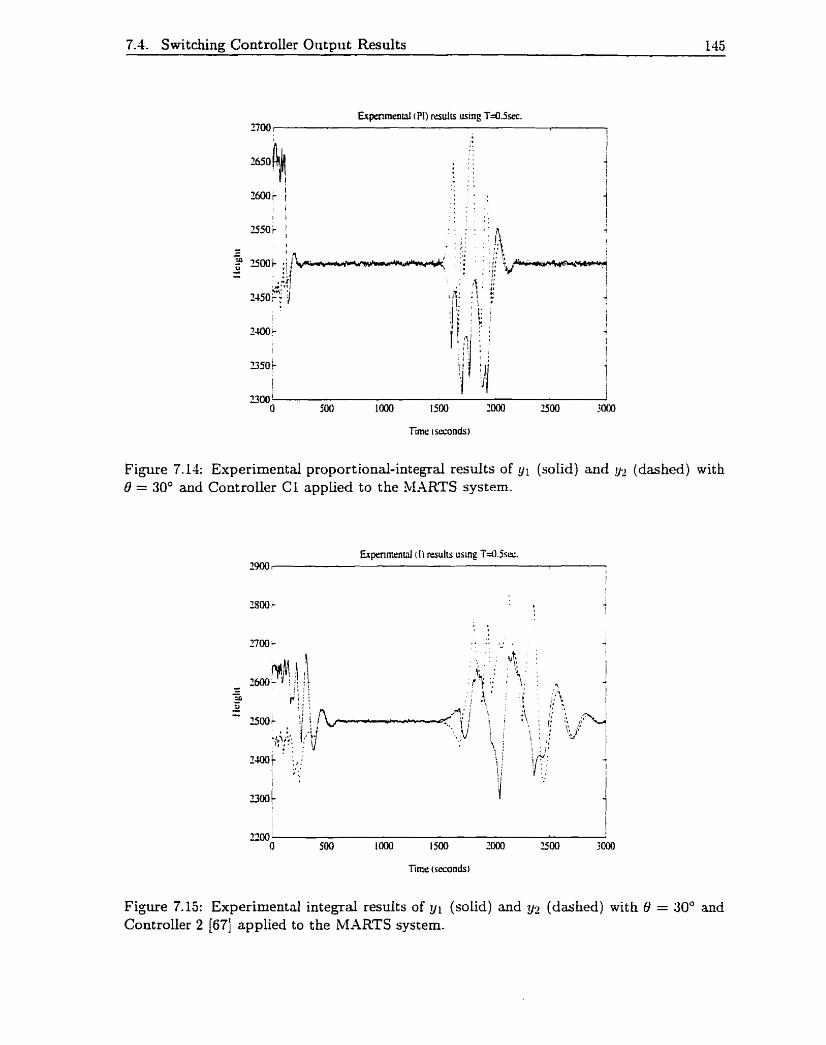
7.4. Switching Controiier Output Results 145
Figure 7.14: Experimental proportional-integrd results of 91 (solid) and yr (dashed) with 8 = 30" and Controller C l applied to the MXRTS system.
Fiogre 7.15: Experimental integrai results of y1 (solid) and y2 (dashed) with O = 30° and Controuer 2 [67] applied to the MARTS system.
Chapter 8
Conclusions
In this chapter. the main contributions of this work are Iisted. and possible future resemch
directions are discussed.
8.1 Summary of Results
In t his t hesis. a new class of switching controllers using a variant of the switching mechanism
originally presented by Miller and Davison in [64! has been constructed to solve a number
of problems in which as little a pr ior i plant information as possible is assunied to be known.
For exampie, the following classes of probleuis have be investigated and solved:
a general adaptive switching probIeni for a faniiIy of not rlecessariIy strictly proper
MIMO plants (Chapter 2):
0 an adap t ive stabilizat ion problem for possibly unknown MIMO systems (Chapter 3) :
0 a self-t uning proport ional-integral-derivative (PID) robust servomechanism problem
for constant reference and constant disturbance inputs for stable plants (Chapter 4);
a a self-t uning proport ional-integral (PI) robust se~omechanism probleru wit h control
input constraints for constant reference and constant disturbance inputs for stable
plants (Chapter 5); and
an adap tive servomechanism problem for potent ially unknown MIMO plants (Chapter
6)-
8.2. Future Research Directions 147
As well, al1 controllers developed here are robust with respect to bounded immeasurable
additive noise dis t urbances applied to control signal .u( t ) and/or plant output y ( t ) .
Since one of the main objectives of this work has been to reduce the potentiai closed
loop tuning response through tlie use of as little a priori plant informatio~i as possibie,
the controllers presented here t herefore are significant in the sense t hat, wit h the exception
of Controller Cl , switching now is based partially upon direct norm bounds on the system
output error. Moreover, initial simulation results obtained when using t hese new controllers
tend to indicate that a desirable improvement in the system transient response generally
can be achieved by selecting non-pathological controller and tuning parameters.
An experirnental real-time application study of one such class of switching controllers.
using almost no a prion' plant information when applied to a multivariable hydraulic systeni
(MARTS), indicates that the proposed controllers are feasible to iniplement in ari iridustrial
environment: in fact, i t has been shown that such controllers operate satishctorily in the
presence of extreme structural changes occurring unexpectedly in the plant.
8.2 Future Research Directions
While many of the results presented here are positive. and tlierefore give assurailce as to the
development of a full theory of general adaptive switchirig coritrollen. riuIIieroiis outstaiidiiig
points still reuiain open for future exaniination. For exaniple, althougli switctiiiig now is
based partially upon direct norm bounds ori tlie system output error. an unacccptably
large output transient response may still occur if there exists a large nurnber of candidate
feedback controllers. This situation can be seen in Figures 2.8 and 3.11: and lience. further
investigations into the reduction of initial tuning t rwien t s are warranted.
However, as one example of the potential generality afforded by the faniily of switching
controllers proposed in this thesis. consider the time-varying plai t [56. pg. 111
which is outside the class of systerns considered in this work. Assunie that the plant is
unknown, biit that it is kriown that there exists a zero'th order stabilizirig corriperisator for

8.2. Future Research Direct ions 148
the system (Le. it is known that for some value of Li E R. the cIosed loop system w i l be
stable with u = L a ) . As one can veri&, since the closed loop system may be expressed as
(3 + Li) t (L, - 1) sin(2t) ~ ( t ) = exp +
4
for a fixed value of Li E R: ( A + BL,C) is exponentially stable (in the sense made precise
in [47. pp. 167-1681} if and o d y if Li < -3.
Upon applying Controller S2 and on defining h( i ) as
wit h
the sample output responses given in Figures 8.1 and 8.2 are obtained for the case when
x ( 0 ) = 1 aud ~ ( 0 ) = 0.001 respectively. Since successtiil controI occurs? it therefore is
conjectured that subsequent extensions of these coritrollers to various cluses of linear time-
varying systems may also be conceivable.
Indeed, using the many weU known techniques that have been applied so successfully to
conventional mode1 reference adaptive control problems. it may likewise be advantageous to
replace bounding function /(k) by a dynaniic one. j? where j would have certain resetting
properties (during time periods when no further switches occur) and could possibly be
governed by the general nonlinear different ial equat ion

8.2. Future Research Direct ions 149
Time c seconds 1
15 1 Controller K u versus urne.
1
" O I 3 J 5 6 7
Timr (seconds)
Figure 8.1: (x (0 ) = 1) Sirnulated results with Controller S2 applied to (8.1) using (8.2) with x (dashed) and y (solid).
3 0 0 7 Thmreiicai conmuous urne switchine conuoller results.
1
15 Controlla K v vmus umc 1
Timr (seconds)
Figure 8.2: ( x ( 0 ) = 0.001) Sirnulated results with Controller S2 applied to (8.1) using (8.2) with x (dashed) and y (solid).

8.2. Future Research Directions 150
F u t hermore. due to the simplistic switching mechanisrns proposed in t his t hesis. addit ional
improvements in the current transient tuning response (through. for instance. the use of a
more complex switching structure and/or increased a priori system informat ion) also are
surmised to be viable in aay future work.

Appendix A
Proofs of Main Results
In this appendiu. remaining detailed proofs of the main results presented in CIlapters 2. 3,
and 4 are given.
A.1 Adaptive Switching Control of LTI MIMO Systems
A L 1 Theorem 2.1
Proof: The proof is by contradiction. and essentially works by constructing a Luenberger
observer to estimate the unknown plant state z( t ) . üsing norm bounds on controller state
7 7 ( t ) as well as u priori properties of the bounding function f . a contradiction can t hen be
shown to occur.
The proof proceeds in the following four phases:
Phase I obtains a bound on the observer error:
me Phase 2 obtains a bound on the estimated plant states:
Phase 3 obtâins a bound on the augmented p l a t and controlIer states: and
Phase 4 uses a priori properties of bounding function f and Lemma 2.1 to show that
a contradiction occurs.
Phase 1: To prove property i): assume that there exist a controlIer parameter f E MSBF.
a continuous reference yrej having norm a continuous disturbance w having norni 6,
and an initial condition z (0 ) = [ x ( o ) ~ D ( ~ ) T ] T for which Assumption F1 liolds' but property
A.1. Adaptive Switching Control of LTI MIMO System 152
i) does not: it follows that ti is defined for al1 i E N. Furthermore,
for some constant m E {1 ,2 , . . . , s}.
Since (Cm, A,) is detectable, this irnplies that there exists a matrix fi such that X(A, + MC,) c @-. Hence, one can [theoretically) construct a (full order) Luenberger observer
of the form
with I ( t i ) an arbitrary constant vector in Pnrn and X(A, + MC,) C @-. Also? with
t herefore
e = 2 - 5
= ( A , +-GfC,rt)é
and
for t E ( t l , t , ] , p E N, p 2 2. Upon recalling that the stability of niatrix (A, + iGC,)
irnplies tha t there exist constants (6, -X) E Pi x Ri so that ~ l e ( " ~ n ~ " ~ ~ ) ' l l 5 ireit for
t 2 0, it follows (after taking norms) t hat for t E (t ,, t,],
Phase 2: Similarly, since

A.1. Adaptive Switching Control of LTI MIMO Systems 153
t herefore
upon defining
and on noting that
for t E ( t l : t,]? it also follows that
Phase 3: Now iising the fact that
and thus that
A.1. Adaptive Switchinn ControI of LTI hIIb10 Systems 154
for t E ( t i . t p ] : it t herefore follows that
for t E ( t l . t,] and for finite constants CO > O. ci > 1. In addition. because
t here fore
for t E ( t l : t,].
Phase 4: Since Lemma 2.1 holds for al1 siich tiiat ( ( j - 1) mod s) = nr - 1. ;iiid sinçe
f E WSBF, tliere exists a finite j _ ( ( j - 1) mod s) = rn - 1. sricii that
(ii) c31'(3) + C < f ( j )
are both satisfied for t E ( t ; : t ;_ ,]: if we now set t = t ;_ , : tiieii t lie iiieqtialit ics
contradict our definition of t;+,: tience property i) is true.
From property i) and the bound given in (AI) , property ii) follows: also. from i): there
exist matrices Gss, Hss, Jss, K,,, L,,, M,,, and a t,, 2 O such that (G(t), H ( t ) , . i ( t ) ,
K ( t ) , L ( t ) ! iW( t ) ) = ( G s s , Hss, J,,. Kss, L,,: rLI,,) for al1 t > t,,; it therefore follows from
Proposition 2.2 that for almost al1 (Gi, Hi, Kt, Li)? Ai will Iiave no eigenvalues in CO ; Lience.
property iii) follows since for almost all (Gi, Hi, Ki$ Li), tiie excited modes of t lie final closed
loop system will be stable. 0
Proof: To prove property i): assume that there exist coritroller parameters E MSBF
and X E R+. a piecewise continuous reference g , , ~ Iiaving norm a piecewise continuous
disturbance w liaving norm W. and an initial coridition Z(0) = [ X ( O ) ~ r l ( ~ ) T el(0)']* for
which Xssumption F2 holds? but property i) does iiot: it follows that t , is <hfined for ail
i E N. Furthermore,
P € P P=P*
for some constant rn E { 1 .2 . . . . . s ) : as such. for t E (tp-l? t,]: p E N. p 3 2. it also follows
where x ( t G l ) = x(tP- 1).
and
Since (Cm, A,) is detectable. consider the partial state estimation problein [18. pg. 3611
A. 1. Adaptive Switching Control of LTI MIMO Systerns 156
given by
for t E (t,- ,, t,]. Upon setting
on noting that
and upon defining
it therefore follows that

A. 1. Adaptive Switching Control of LTI bIIMO Systems 157
w here
In addition, by rewriting (-4.2) as
and on defining
t herefore
Now since (Cm, 4,) is detectable. let matrix &! I>e chosen sucli that A(-& + ,@cm) c
@-. Observe tliat (Agl, A;'~) is detectable for al1 p My p > 2. and consider
A.1. Adaptive Switchin~ Control of LTI PvITiLIO Systems 158
for t E ( t p - 1. t,] with 2( t i ) an arbitrary constant vector in Rnm and A(.-$', i (;p-lji<l) =
A(-& + MC,) c C-. Also. with
t herefore
and
for t E ( t l ' t,]. Upon recalling that the stability of matriu (-4, + -F~C,) iniplies that there
exist constants (6 . - A ) E Rf x R- so that / le(-4m'"Cm)t~~ < 6eXt for t 2 0. it bllows (after
taking norms) that for t E ( t i . t p ] .
Similady. upon defining
A. 1. Adaptive Switching Control of LTI MIMO Systems 159
for t E (t,-l? $1, and on noting that
t herefore
however, since
for t E ( t 1, t,], and witli
it also follows tfiat
Now using the fact that
4 'ri

A.2. Adapt ive Stabilization of LTI Systems 161
From property i) and the bound given in (A.3). property ii) follows: &o. from i): there
exist matrices G,,, H,,, J,,? K,,? L,,, iMSbgI,,: and a t,, 2 O such that (G( t ) . H ( t ) . . J ( t ) .
K ( t ) , L ( t ) , iU( t ) ) = (G,,? Hssl*Jss. K,,. L , , . M 9 , ) for dl t > t,,; it therefore follows from
Proposition 2.2 that for almost al1 (Gi, Hi: K t , L,): Ai will have no eignvalues in Co: hence.
property iii) follows since for almost al1 (Gi: Hi , K,. Li), the excited modes of the final closed
loop system will be stable. U
A.2 Adapt ive Stabilizat ion of LTI Syst ems
Proof: To prove property i ) ? assume t hat there exist controller parameters f f S LBF and
( E ~ , T) E S: a continuous disturbance w having norm G. and an initial condition z(0) for
wbich Assumption S 1 holds. but property i) does not: it follows that t , is defined for d l
i @Ne
Since
a d c + 0: therefore
for dl t 2 O. As weil, using the fact that
for t E ( t I , t,], p E N, p 2 2. it therefore follows that

A.2. -4dapt ive Stabilization of LTT Systems 163
for t E (tlT t,] and for constants (co.cl) E B' x X'.
Consider now a j' sufncient ly large so t hat Lemma 3.1 holds for al1 q 2 j . t E ( t,. t,[,
with ( ( q - 1) mod 2) = ( ( j ' - 1) rnod 2). Since f E SlBF. there exists a finite > ;. ((3 - 1) rnod 2) = ((j - I ) rnod 2). such that Lemma 3.1 holds and
I Y ( ~ ; + J < f (3
contradicts our definition of t j T I ; hence property i) is mue.
Rom property i) and the bound given in
exist an E,, E R'. K,, E {l. -1}. and a t,, ..-t
al1 t 3 t,,. Since K,, E K and E,, = for 50
for almost di T ) E S. ( a + ~E, ,K , , c ) # O:
(A.4). property ii) follows: also. from i) . there
2 O such that ~ ( t ) = E,, and K ( t ) = K.%, for
some i E W. it follows from Remark 3.1 that
hence property iii) foIlows since for almost al1
(€0 . T ) E S. the excited modes of the final closed loop system will be stable.
A.2.2 Theorem 3.2
Proof: To prove property i). assume that there exist cnntroller parameters f E S3BF and
h E CTF, a continuous disturbance cu having norm W. and an initial condition = ( O ) = [r (O)=
~ I ( o ) ~ ] ~ for which .Assumption S2 holds. but property i) does not: it foliows that t , is defined
for al1 i E !Y.
Since (C. A) is detectable. this implies that there exists a niatr~u such that A(-4 i
MC) C @-. Hence. one can (theoretically) construct a (full order) Luenberger observer of
the form
ii = (A+iîdC)?+ Bu - M y + ( E + M F ) w
with Z( t i ) an a r b i t r q constant vector in Rn and X(A t MC) C C-. Also. with
A.2. Adaptive Stabilization of LTI Systems 163
t herefore
and
for t E ( t l : t ,] , p E PI, p 2 2. Upon recalling that the stability of matriw ( A + MC) implies
that t here exist constants (a. -X ) E 8' x P' so t hat le('\+."")^ 11 < - de*' for t 2 O. it follows
(after taking norms) that for t E ( t t,].
t herefore
upon defining
a~id on noting that
Ilv(t)ll I f b - 1)
and Ilu(t)ll <- .<-'f @ - 1) + f @ - 1 )
A.2. Adap tive Stabilizat ion of LTI Systems 164
for constants (q'n) E IR+ x Ri and for t E ( t l : t p ] , it also foUows that
0 11 5 a .. ll*(t i ) l l + 2 (mi (TP-' f @ - L) + <-If (p - 1)) + m J ( p - 1) + mniü) . 1x1
Now using the fact that
and thus that
for t E ( t : t,]: it t herefore Follows t bat
For t E ( t l . t,] and for finite constants ca > O. ci > 1. Q > 0. r > O. In addition. because
t herefore
(A..)
for t E ( t l , t ,] .
Since h E CTF, and since it is known that gi = q will stabilize (3.2). where q E N U { O ) :
for some ci E ~ ( ~ ' g ~ ) ~ ( ' ~ ~ ~ ) . consider now a j' sufficiently large so that Lemma 3.2 holds
for t E (t;. t;,,]: with f E S2BF and h E CTF, there therefore exists a finite J' 2 j' such
t hat Lemma 3.2 holds and
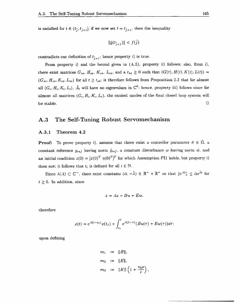
A.3. The Self-Tuning Robust Servomechanism 165
is satisfied for t E ( t ; , t ; + l ] ; if we now set t = t;, , , tlien tlie inequality
contradicts our definition of t;, : Lience property i) is true.
From property i) and the bound given in (A.5). property ii) follows: also. from i),
there exist matrices G,,, Hss, Kss. L,,, and a t,, > O such that (G( t ) . H ( t ) . K ( t ) ? L ( t ) ) =
(G,,. Hss7 K,,. L,,) for al1 t 2 t,,; it therefore follows frorn Proposition 2.2 tliat for alrnost
al1 (Gi, Hi , l(,' Li) rIi will have no eigenvalues in @O: tience. property iii) follows sirice for
almost al1 matrices (G,, Hi, KI, L,). the excited modes of the filial closed loop systern will
be stable. 0
A.3 The Self-Tuning Robust Servomechanism
A.3.1 Theorem 4.2
Proof: To prove property i). assume tliat there exist a controller paranieter 5 E fi. a
constant reference gr,== Iiaving norrn ire!. a constant distiirbaiicc io Iiaviiig norni iü. niid
a n initial condition z (0 ) = [z(o)* l l ( ~ ) T ] T for wliich Assumptioli PI1 Iiolds. 1)ut property i)
does not: it follows tliat t , is defiued for al1 i E P!.
Since X ( A ) c C-. ttiere exist constants ((5. -X) E 2- x 8' so tliat lJe''tJl 5 GeAt for
t > O. In addition. since
i = .+lx t Bu i Ew.
upon defining
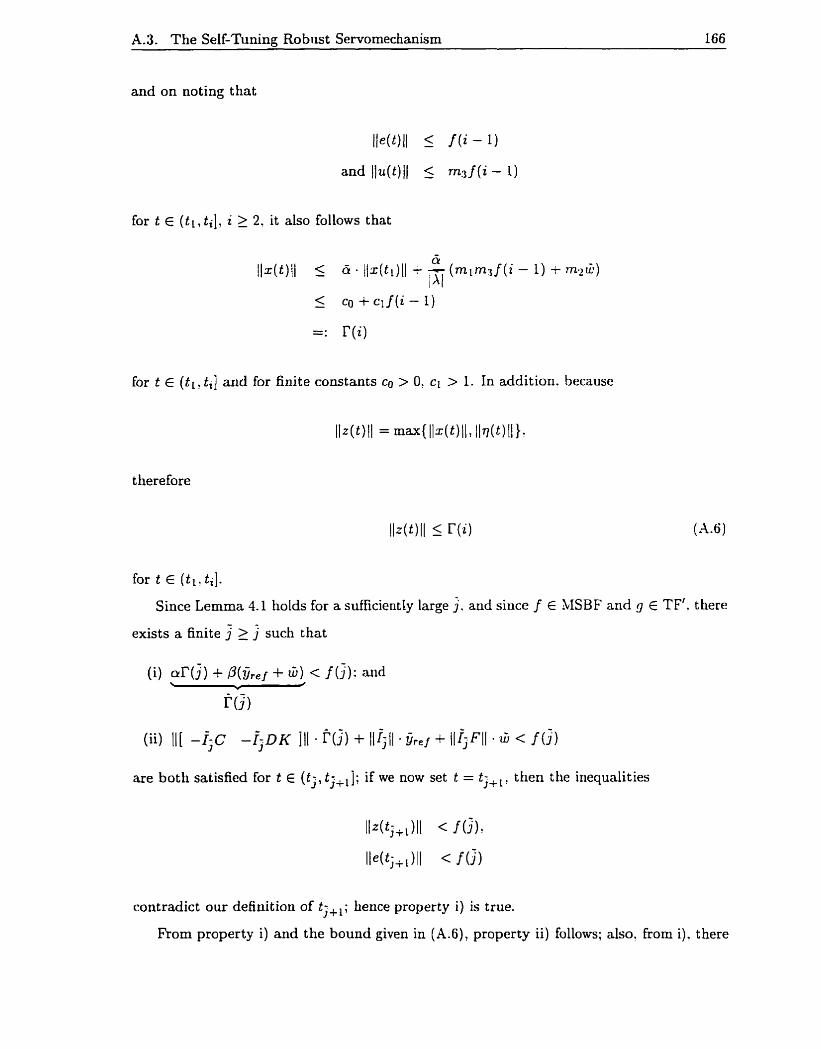
A.3. The SeIf-Tunine: Ro bust Servomechanism 166
and on noting that
for t E ( t l , t i ] , i 3 2. it also follows that
for t E ( t l , ti] and for finite constants co > 0. ci > 1. In addition. because
t herefore
for t E ( t i , t i ] .
Since Lemma 4.1 holds for a sufftciently large 3. and since f E MSBF and g E TF'. there
exists a finite 3 2 3 such that
(i) d ( j ) + P(,j,,, + G) < f (j): and
are both satisfied for t E (tj , t;+,]; if we now set t = t;,,, then the inequalities
contradict our definition of t;,,; Lence property i) is true.
Rom property i) and the bound given in (A.6) , property ii) follows; also. from i), there

A-3. The Self-Tunine: Robust Servomeciianism 167
€0 exist an E,, E !Et+ and a t,, 2 O such that c ( t ) = es, for ail t > t,,. Since es, = - for
some i E W, it follows from Lernma 4.2 that for almost al1 (Q, T) E S. A(p. c,,) will have
no eigenvalues in @O; hence, property iii) follows since for alrnost al1 (eo7 T) E S. the excited
modes of the final closed Ioop system will be stable. 0
A.3.2 Theorem 4.4
Proof: Although the proof of Theorem 4.4 is very similar in nature to that provided for
Theorem 4.2, it will nevertheless be given in complete detail. To prove property i). assume
that there exist a controller parameter a p l ~ E ClPIDI a constant reference y,,! having norm
grel: a constant disturbance w having norm 6, and an initial condition z(0) = [z(OIT q(0)T
a ( ~ ) ~ ] ~ for which Assurnption PIDl holds? but property i) does not: it follows tliat t i is
defined for a11 i E N.
Since X(A) C C-. there exist constants (& ' -A) E R' x P' so that I ~ ~ " ' I I 5 ~ e " for
t > O. In addition, since
t herefore
upon defining
and on noting that

A.3. The Self-Tuning Robust Servomechanism 168
for t E ( t l ? t i ] , i 2 2, it also follows that
for t E ( t i , ti] and for finite constants CO > 0: ci > 1. In addition. because
t herefore
for t E ( t l , t i ] .
Since Lemma 4.4 holds for a sufficiently large 3, and since / E MSBF and ( g . g1 , g2) E
TF' x TF' x TF', there exists a finite 3 2 j' such ttiat
(i) al?(;) + + fi) < f ( j ) ; and
( i ) [ - -Ï;DK 9 2 ( j ) ~ 2 Ï j ~ ~ ] I I - ~ ( ~ ) + I I I - P ~ ~ ( ~ ) ~ ~ D K I I - G ~ . ~ + I ~ ~ ~ F I I . @ < f ( 3 )
are both satisfied for t E ( t j , t; , ,]; if we now set t = tj+,: then the inequalities
contradict our definition of t ; + [ ; tience property i) is true.
From property i) and the bound given in (A.7), property ii) follows; also, from i) , there
exist ( e s , , e , , , ,c , , , ) E W+ x Et+ x WC and a t , , 2 O such that e ( t ) = es,, c i ( t ) = c,,,, €0 € 0 2 and t p ( t ) = c,,, for al1 t > t,,. Since es , = -, es , , = 3 aud ess2 = - . for some rL ri ' 7.;
i E N, it follows from Lemma 4.5 that for almost al1 ( t g , T , €0, , ~ 1 ? eo2, r2) E S x S x Si
À P I D ( P 7 es,, t,,, , es,, , K, N) will have no eigenvalues in CO; Iierice, property iii) follows since
for almost al1 (ea, T , EO,, 71, C O - , T ~ ) E S x S x S, the excited riiodes of the filial closed loop
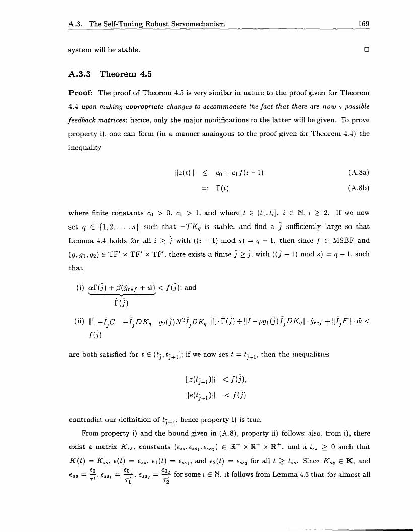
A.3. The Self-Tuning Robust Servomechariism 169
system will be stable.
A.3.3 Theorem 4.5
Proof: The proof of Theorem 4.3 is very similar in nature to the proof given for Theorem
4.4 upon making appropriate changes to accommodate the Jact that there are now .s possible
feedbnck mutrices: hence. only the major niodifications to the latter wiI1 be given. To prove
property i ) , one can form (in a manner anaiogous to the proof giveri for Theorem 4.4) the
inequality
where finite constants CO > O, ci > 1. and where t E ( t l : tijl i E M. i >_ 2. If we now
set q E {l. 2 . . . . . s } such that -TK,, is stable. and find a siifficiently large so that
Lemma 1.4 liolds for al1 i 2 3 witli ((i - 1) tiiod s ) = q - 1. ttieri since f E SISBF and
(9, gi.y2) E TF' x TF' x TF'. tliere exists a finite j 2 ;. witti ( ( j - 1) n i d s ) = q - 1. sticli
t hat
(i) d ( j ) + + 6 ) < f ( j ) : and
are both satisfied for t E (t;. t;,, 1; if we now set t = tj,,, tlien the iricquülitics
contradict o u definition of tj,,; hence property i ) is true.
Rom property i) and the bound given in (A.8): property ii) follows: &o. from i)? there
exist a matrix Kss, constants (es,, E . ~ ~ ~ . esS2) E B- x Bi x Rf . and a t,, 3 O siich that
K ( t ) = K.ss, ~ ( t ) = es,, c l ( t ) = essi, and ~ ( t ) = es,, for d l t 2 t s s . sincc Kss E K, and €0 €0 1 €O2
cSs = - Ti cssl = -, csSl = - for some i E N. it follows fiom Lemrna 4.6 that for alrnost al1 7: r;

A.3. The SeIf-Tuning Robuçt Servomechanisrn 1 70
(sa, T' , T I ' €a2. T2, U) E S x S x S'. A p l D ( p o Easi c,,, ? K,,. N ) will have no eigenvalues
in cor hence, property iii) foiiows since for alrnost al1 (€0 . T. €0, - ri? col: 72. Lr) E S x S x Sf7
the excited modes of the final closed Ioop system will be stable. Cl
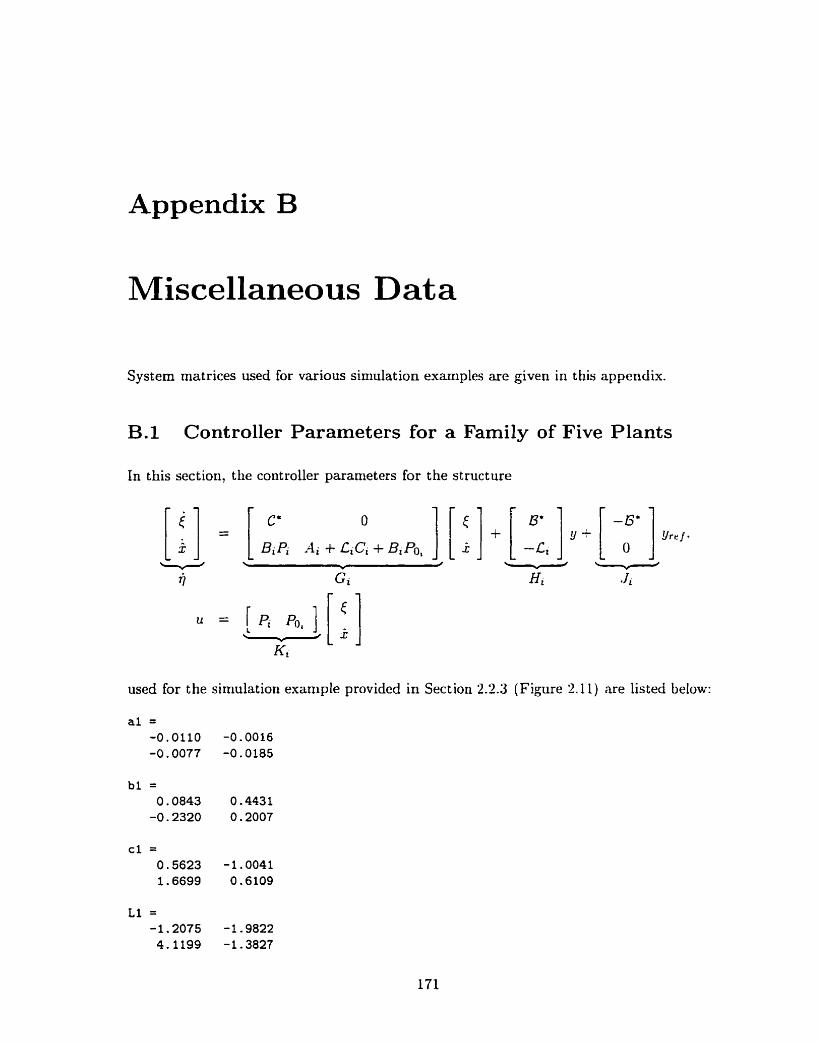
Appendix B
Miscellaneous Data
System matrices used for various sin~ulation examples are given in this appendix.
B.1 Controller Parameters for a Family of Five Plants
ln this section, the controller parameters for the structure
used for the simulatiori example provided in Section 2.3.3 (Figure '2.11) are listed below:
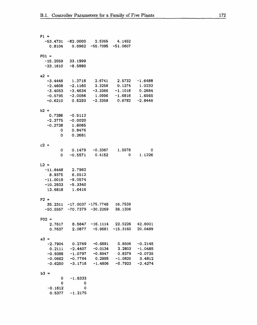
B.1. Controller Parameters for a Family of Five Plants 172
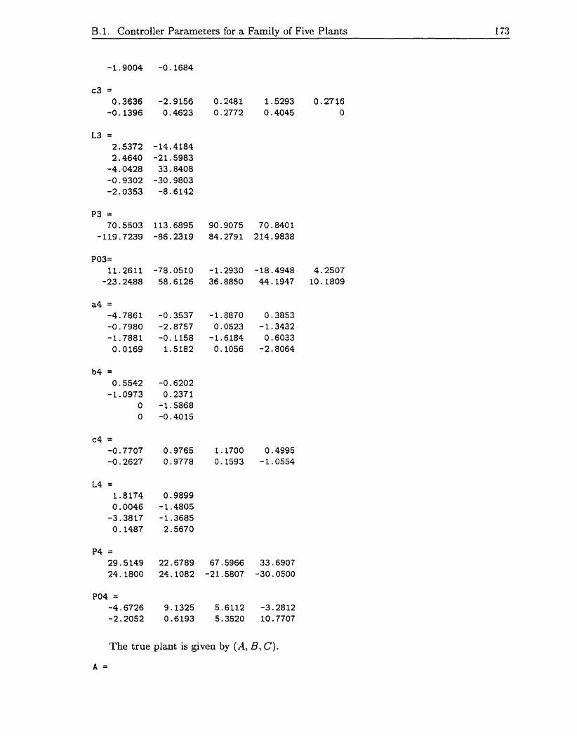
B. 1. Controller Parameters for a Family of Five Plants 173
The true plant is given by ( A , B? C).
A =
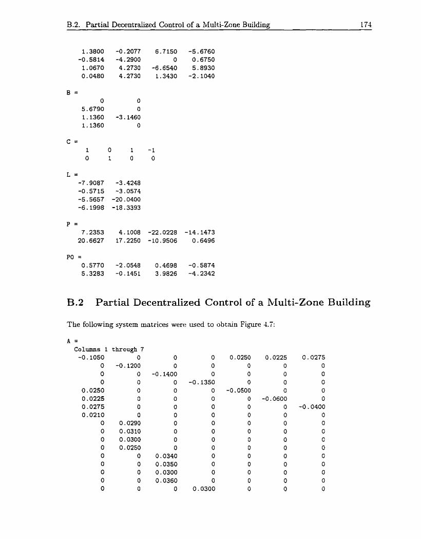
B.2. Partial Decentraiized Control of a hduiti-Zone Building 174
B.2 Partial Decentralized Control of a Multi-Zone Building
The following system matrices were used to obtain Figure 4.7:
A = Columns 1 through 7
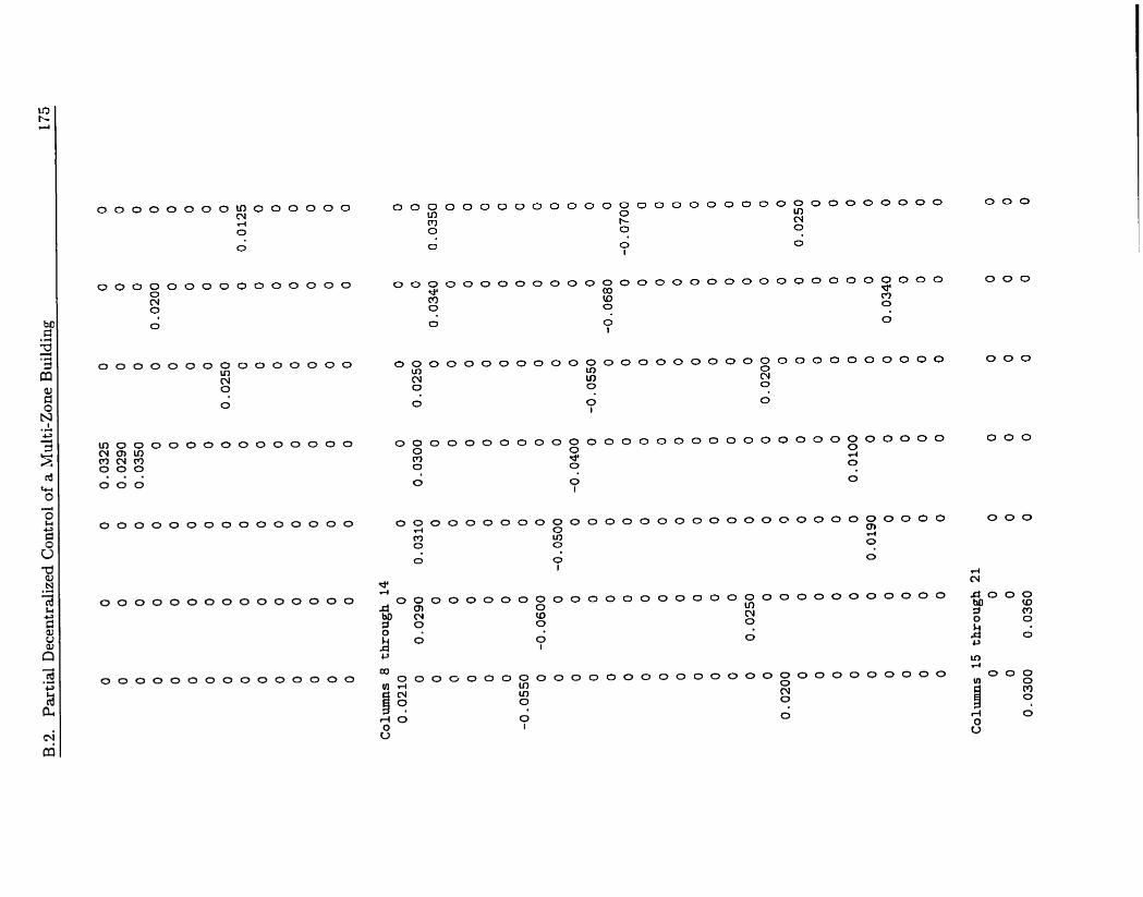

B.2. Partial Decentralized Control of a Multi-Zone BiiiIdin~
Columns 22 through 28

B.2. Partial Decentralized Control of a Multi-Zone Building
Columns 29 through 32
Columns 1 through 7 O O
Columns 8 through 14 O O O
Columns 15 through 21 O O O

B.3. A Four Input-Four Output Furnace Model 175
Columns 22 through 28 O O O 0.0070 0.0050 0.0050 0.0060
Columns 29 through 32 0.0060 O. 0060 O. 0045 O. 0050
A Four Input-Four Output Furnace Mode1
The following matrices were used in the simulation to obtain Figure 4.9:
A-R = -0.2003 -0.0044 O. 0002 O. 0008 o. O000 o. O000 0.0000
B-R = -0.5606 -0.4696 -0.5579 O. 76% -0.1268 O. 3292 O. O658
C-R = -0.1154 -0.1498 -0.1628 -0.1303
D-R = 0.0042 -0.0002 -0.0059 0.0015
E-R = o. 1000 o. 1000 0.1000 O. 1000 O. 1000

B.3. A Four Input-Four Output Furnace Mode1 179
These matrices were obtained upon using the mode1 reduction methods given in [26] on
the original furnace mode1 given in [!IL. pg. 1991 and !26jL. The system matrices
obtain Figures 4.10 and 4.11 are Iisted below.
A = Columns 1 through 7 -0.2323 O. 0023 0.0067 O. 02% O. 0055 -0.0224 -0.0572 -0.00 18
Column 8 O. 0045 -0.0123 O. 0057 0.0073 -0.0055 o. 0020 -0.0003 -0.2038
B = -0.3339 -0.1606 O. 1476 O. 1986 -0.1571 O. 0764 -0.0196 -0.0376
C = Columns 1 through 7 -0.4177 -0.3583 -0.3344 -0.2647 -0.4481 -0.1575 -0.3225 O. O 137 O. 3904 -0.2685 0.2041 -0.2276
used to
'ln essence, the system given by (4.14) wm formuiated for didaçtic purposes with DR # 0.
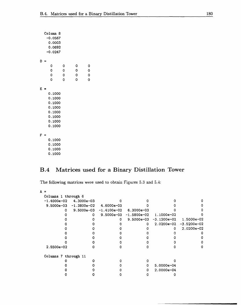
B.4. Matrices used for a Binary Distillation Tower
B.4 Matrices used for a Binary Distillation Tower
The folIowing matrices were used to obtain Figures 5.3 and 5.4:
A = Columns 1 through 6 -1.4000e-02 4.3000e-03 9.5000e-03 -1.3800e-02
O 9.5000e-03 O O O O O O O O O O O O O O
2.5500e-02 O
Columns 7 through 11 O O O O O O O O

B.4. Matrices med for a Binarv Distillation Tower 181
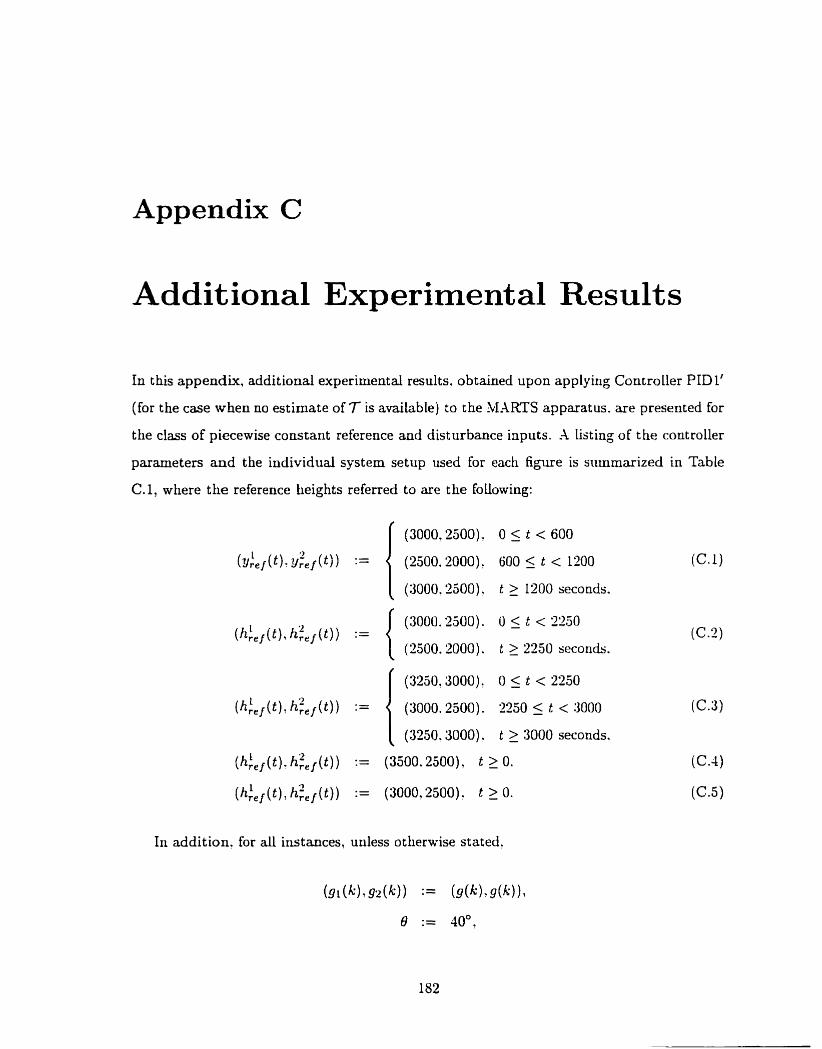
Appendix C
Addit ional Experiment al Result s
In t his appendix, additional experimentd results. obtained upon applying Controller PID 1'
(for the case when no estimate of T is available) to the SIXRTS apparatus. are presented for
the class of piecewise constant reference and disturbance inputs. A listing of the controller
parameters and the individual system setup used for each figure is siimmarized in Table
C.1, where the reference Lieights referred to are the foilowing:
(3000.2500), O 5 t < 600
Y Y ( (2500.2000). 600 5 t < 1200
(3000.2500), t 2 1200 seconds.
(3000.2300). O 5 t < 2250
(2500.2000). t 3 2250 seconds.
1 (3250,3000). O 5 t c 2250
h . h ) := (3000.2500). 2250 5 t < 3000
(3250.3000). t >_ 3000 seconds.
( t ) h t ) := (800.2500)' t 3 0.
(hfe ( t ) : hp, ( t ) ) := (XIOO. 2500). t 2 0.
In addit ion, for al1 instances, uriless ot herwise stated,

C. Addit ional Experimental Results 183
and T := 0.75 seconds.
Table (2.1: Summary of the parameters used for Figures C.1-C.12. wliere o ( k ) :=
floor (y) a d ( k ) := 5 - (((k - 1) mod 6 ) + 1)-
1015" O 5 -4 LVl 'i 10/5" O 15 4 ?j Y (CA) - 10/3O O 3 6 \VI Y/Y (CA) -
Additional notes and comrnents:
10/3" 10/3" 10/3" 10/3"
(a) Iri Figures C.11 and C.12. output leads y i ( t ) and p ( t ) are reversed at t = 2250
seconds.
20 20 20 20
3 20 3 3
10/3" 20 10/3" 1 3
20 5 20 10
10/5" 10/za
6 5 6 5
20 20
5 6 4 4
ttVl tVt
1
11,
?3 S 'r' Y 1- Y
Y/?- (C.3) / X/E' X/Y
/ N/X / (C.2) N/Y (C.3) -
(CA) (CA)
Y I ( 4 (a)
- -
S/N j (c-5) (a) [
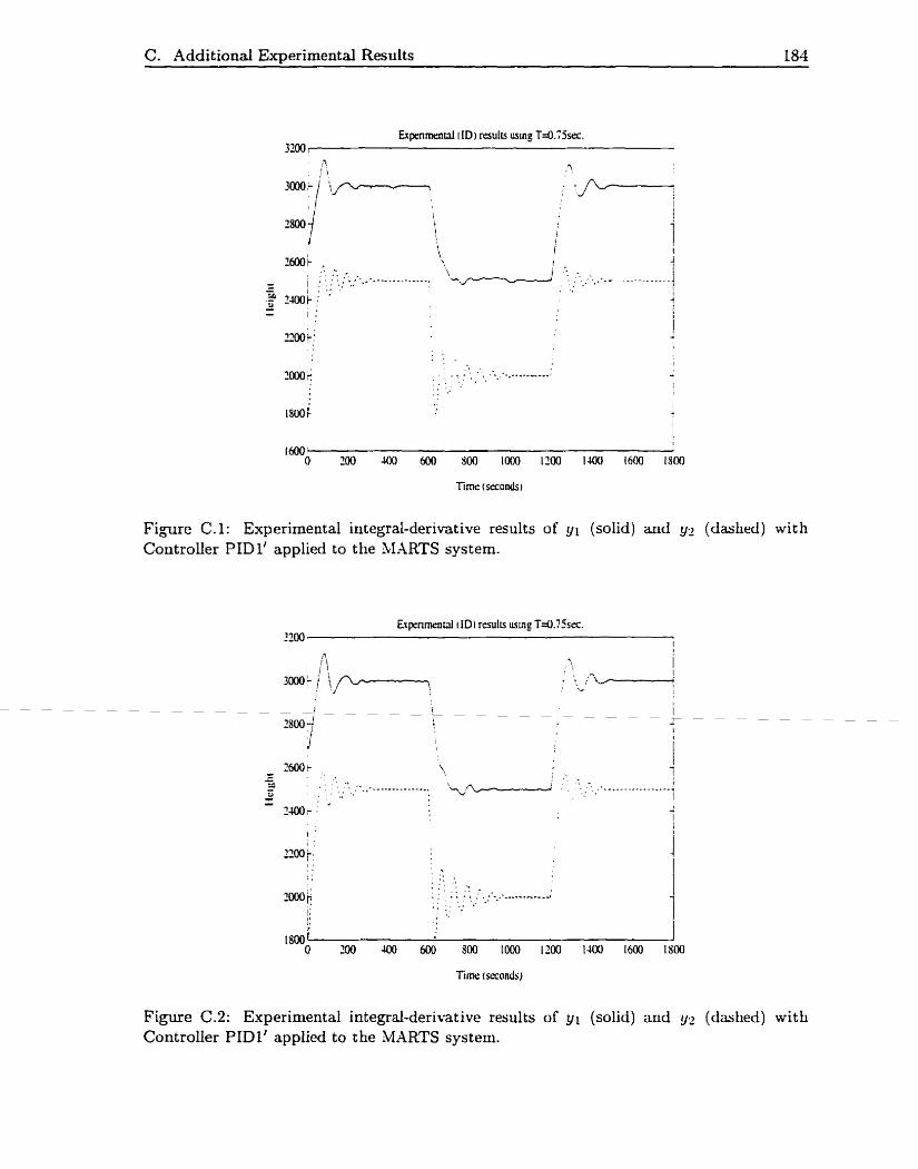
C. Additional Experimental Results 184
Fiorne C. 1: Experimental integral-derivat ive results of y 1 (solid) and y- (dashed) wit h Controlier PID1' applied to the MXRTS system.
fime (seconds)
Figure C.2: Experimental integral-derib*at ive results of y 1 (solid) and y2 (dashed) wit h Controlier PIDI' applied to the MARTS system.
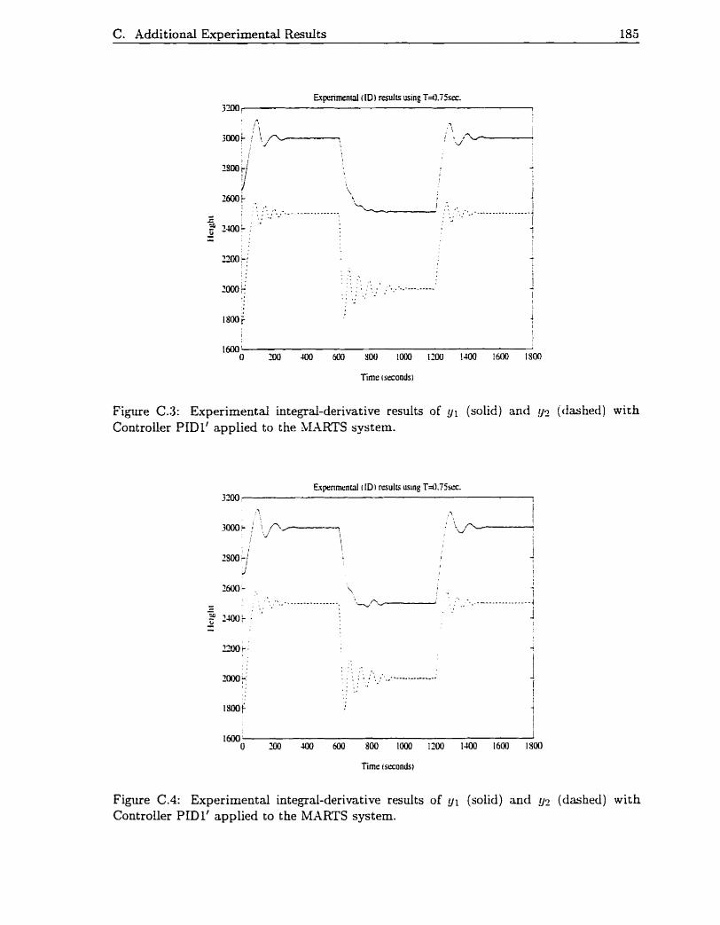
C. Addit ional Emerimental Results 185
Figure C.3: Experimental integral-derivative results of y1 (solid) and fi (dashed) wi th Controller PID1' applied to the MXRTS system.
Expenmrnul (ID i rcsults usine T 4 . 7 5 ~ ~ . 3100 : I
Figure C.4: Experimental integral-derimtive results of y1 (solid) and 12 (dashed) with Controller PID1' applied to the MARTS system.
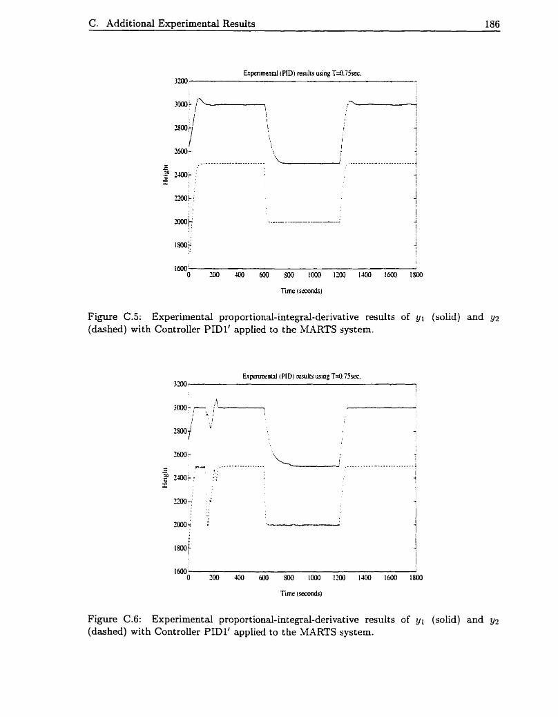
C. Additional Experimental Results 186
fime i seconds )
Figure C.5: Experimental proportional-integral-derivative results of y1 (solid) and y:! (dashed) with Controller PID1' applied to the MARTS system.
1
1600' I O 7 0 UXI 600 $00 lûûû 1700 1100 1600 1800
Timr (seconds)
Figure C.6: Experimental proportioual-integral-derivative results of y1 (solid) and y:! (dashed) with Controiler PID1' applied to the MARTS system.

C. Additional Experimental Results 187
Timt: (seconds)
Figure (2.7: Experimental proportional-integral-derivat ive results of hl (dashed) and h2 (solid) wit h Controller PID 1' applied to the reversed MARTS system.
1 5 0 0 ~ 1 O 500 Io00 1500 Zoo0 300 3000 3500 U)c]O
Time (seconds)
Figure C.8: Experimental proportional-integral-derivat ive results of h 1 ( d a . hed) and hs (solid) wit h Controller PID 1' applied to the reversed MARTS system.

C. Addit ional Emeriment al Results 188
Loo-
1000 -
Figure C.9: Experimental proport iond-integral-derivative results of h i (dashed) and hz (solid) wit h Controuer PID 1' applied to the reversed MARTS system.
Time (srconds)
Figure C. 10: Experimental proport ional-integral-derivat ive results of h (dashed) and h2 (solid) wit h Controller PID1' appiied to the reversed MARTS systeui.
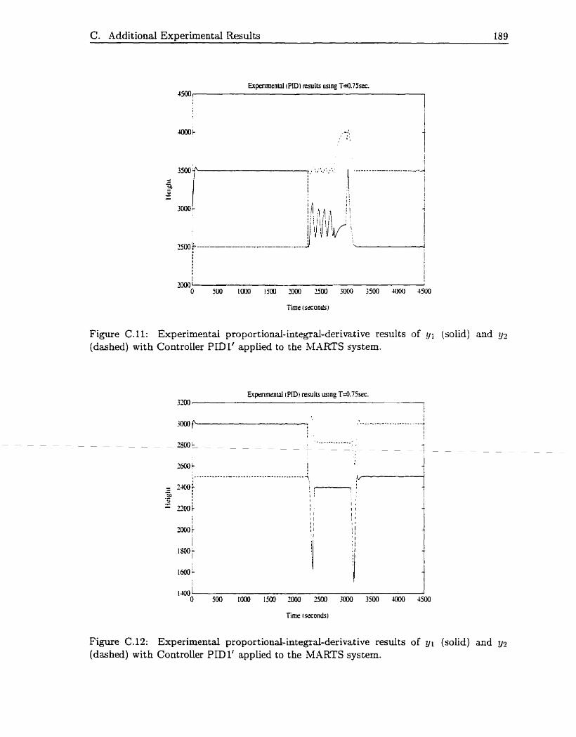
C. Additional Experimental Results 189
Time (seconds)
Figure C. 11: Experimentd proportional-integral-derivat ive results of 91 (solid) and 92 (dashed) with Controller PID1' applied to the MARTS system.
Figure C. 12: Experimentd proportionai-integrai-derivat ive results of $1 (solid) and y2 (dashed) with Controuer PIDI' appiied to the MARTS system.
Bibliography
[l] D. Y. Xbramovitch and G. F. Franklin. On the Stability of Adaptive Pole-Placement
Controllers with a Saturating Xctuator. lEEE Transactions on .4~rrtomatic Control.
35(3):303-306. bIarch 1990.
[2] D. Y. hbramovitch. R. L. Kosut. and G. F. Franklin. Adaptive Coritrol witli Satu-
rating Inputs. In Proceedings of the 25'th IEEE Conferencc on Decision und Control.
pages 848-852. 1986.
[3] B. D. 0. Anderson. Adaptive Systems. Lack of Persistency of Excitation and Bursting
Phenornena. Automaticu. 21 (3) :X7-258. blay 1985.
[il] A. 41. .~~inaswamy and S. P. Karason. Discretotime -4daptive Coritrol in the Prcsence
of Input Constraints. ,-l~utomuticu~ 3l(lO): 142l-l-Ul. October 1995.
[5] K. J. hxtirn and T. Hiigglund. Aiitomatic Tuniug of Simple Regilators witli Speç-
ifications on Phase and Amplitude Margins. .4rrtomaticu. Zl(5):6'45-65 1. Scpternber
1984.
[6] K. J. Astrom and T. Hiigglund. .Automutic Tuning of PID Controllers. Instrument
Society of Amcrica. Research Triangle Park. NC, 1985.
[7] K. J. .kstrom, T. Hiigglund. C. C. Hang, and W. K. Ho. Automatic Tuniug and
Adaptation for PID Controllers - A Survey. Control Engineering Practice? 1(4):699-
714, August 1993.
[8] K. J . Astrom and B. Wit tenmark. ..ldaptive Control. Addison-Wesley PublisLing
Company, Reading, Massachusetts? 1989.

B ibliograp hy 191
K. J. Astrom and B. Wittenmark. Cornputer Contmikd Systems: Tlreoq and Design.
Prentice-Hall Inc.. Englewood Cliffs. New .Jersey, 1990.
J. Balakrishnan and K. S. Narendra- Intelligent Control using Fixed and Adaptive
Models. In Proceedings of the 1995 American Control Con ference. pages 597-601.
1995.
V. Blondel. Simultaneous Stabilization of Linear Systems. volume IO 1 of Lecture No tes
in Control and Injormation Sciences. Springer-Verlag, London. 1994.
M. S. Branicky. Analyzing Continuous Switching Systems: Theory and Examples. In
Proceedings of the 1994 Amencan Control Conference. pages 31 10-31 f 4. 1994.
C. 1. Byrnes and J. C. Willems. Xdaptive Stabilization of hlultivariable Linear Sys-
tems. In Proceedings of the 23'rd IEEE Conference on Decision und Control. pages
1574-1577. 1984.
M. Chang. Adaptive Control Xpplied to Unmodellecl IvIultivariable Systems. Master's
thesis. University of Toronto. Department of Electrical arid Cornputer Erigiiicering,
April 1993.
M. Chang and E. .J. Davison. Control of Unknown Systenis iising Switcliing Con-
trollers: an Experimentd S tudy. I n Proceedings of the 1994 =Imerican Control Con-
ference. pages 2984-2989. 1'394.
M. Chang and E. J. Davison. Control of Unknown Systems using Switdiirig Con-
trollers: The Self-Tuning Robust SerwrriecLanism P roblerri. In Proceedings of the
.S>:liTrrl IEEE Conference on Decision and Control. pages 2833-2838. 19'3.1.
M. Chang and E. J. Davison. New Directions in Industrial Control: IutelIigcnt Control
- An Experimental Study Applied to a Multivariable Hydraulic System. In 1. Lasiecka
and B. Morton, editors, Control Problems in Industnj: Proceedings jrom the SIAil1
Sgmposiurn on Control Problems, S u n Diego, California, July, 1994: volume 21 of
Progress in Systems and Control Theonj, pages 65-95. Birkliauser Press. Boston,
1995.
C. T. Chen. Linear Sgstem T h e o q and Design. Holt: Rinehart and Winston, hic..
New York, 1984.

Bibliography 192
[19] K. Ciliz and K. S. Narendra. Multiple Mode1 Based Adaptive Control of Robotic
Manipulators. Ln Proceedings of the 33'rd IEEE Conference on Deczsion and Control.
pages 1305-1310? 1994.
[20] E. J. Davison. Control of a Distillat ion Column wit h Pressure Variation. Transactions
of the Institution of Chernical Engineers, 45:T229-250, 1967.
[21] E. J. Davison. Multivariable Tuning Regulators: The Feedforward and Robust Control
of a. General Servomechanism Problem. IEEE Transactions on .4utomuti~ Control,
21(1):35-47. February 1976.
[22] E. J. Davison. Description of Multivariable Apparatus for Real Time Control Stud-
ies (MARTS). Systems Control Report 8514. University of Toronto. Department of
Elect ricd Engineering, November 1985.
[23] E. J. Davison and Id. Chang. Intelligent Control: Some Preliminary Results. In B. A.
Francis and A. R. Tannenbaum: editors, Feedback Control, Xonlinear Systems: and
Complexity? volume 202 of Lecture Notes in Control and Information Sciences. pages
67-87. Springer-Verlag, London. 1995.
[24] E. J. Davison and T. N. Chang. Decentralized Stabilization :md Pole Assignment for
General Proper Systems. IEEE Transuctions on Automatic Control. 35(6):652-664.
June 1990.
[25] E. J. Davison and 1. J. Ferguson. The Design of Controllers for the !dultivariable
Robust Servomechanism Problem Using Parameter Optimization Llethods. IEEE
Transactions o n ,.lutornatic Contra6 26(1):93-110, Februaxy 1981.
[26] E. J . Davison, W. Gesing, and S. H. Wang. An Algorithm for Obtaining the Mini-
mai Realization of a Linear Time-Invariant Systern and Determining if a System is
S tabilizable-Detectable. IEEE Transactions on Automatic Control, '23 ( 6 ) : 104% 1054,
December 1978.
[27] E. J. Davison and A. Goldenberg. Robust Control of a General Servomechanisrn
Problem: The Servo Compensator. .4utomatica: 1 l ( 5 ) :46 1-471, September 1975.
[28] E. J. Davison and B. M. Scheninger. Perfect Control of the Robust Servornechanism
Problem. IEEE Transactions on Automatic Control, 32(8):689-702, -4ugust 1987.
[29] E. J. Davison and A. Solomon. Partial Decentralized Temperature Control of Multi-
Zone Buildings. in Proceedings of the 22'nd IEEE Conference on Decision and Con-
trol, pages 10-16, 1983.
[30] E. .J. Davison and S. H. Wang. Properties of Linear Time-Invariant Multivarisble
Systems Subject to Arbitrary Output and State Feedback. IEEE transaction^ on
.4utomatic Control, 18(1):24-32, February 1173.
[31] E. J. Davison and S. H. Wang. Properties and Calculation of Transmission Zeros
of Linear Multivariable Systems. In F. Fallside, editor. Control System Design by
Pole-Zero Asszpment . pages 16-42. Academic Press. New York. 1977.
[32] P. L. Falb aod W. A. Wolovich. Decoiipling in the Des ip and Synthesis of Multi-
variable Control Systems. IEEE Transactions on .;lutornatic Control. 12(ü):651-659,
December 1967.
[33] B. A. Rancis. -4 Course in H, Control Theonj. volume 88 of Lecture Notes i n Control
and Information Sciences. Springer-Verlag, Berlin. 1987.
[34] M. Fu and B. R. Barmish. Xdaptive Stabilization of Linear Systems Via Switcli-
ing Control. IEEE Transactions on =Lutornatic Control. 31 ( 12): 1097-1 103. December
1986.
[35] P. J. Gawthrop. Self-Tuning PID Controllers: Algorithm and Implementation. IEEE
Transactions on .4utomatic Control, 3 1 (3):SOI -209. %faxch 1986.
[36] B. K. Ghosh. Transcendental and Interpolation Methods in Simultaneous Stabilization
and Simultaneous Partial Pole Placement Problems. SIilhf Journal on Control und
Optirnizution, X ( 6 ) : 1091-1 109, November 1986.
[37] G. H. Golub and C. F. Van Loan. .bïutrir Compututions. Jolins Hopkins University
Press, Baltimore, 1989.
[38] G. C. Goodwin and K. S. Sin. Aduptiue Filtering Predzction and Control. Prentice-
Hall. Inc.? Englewood Ciifi. New Jersey, 1984.
[39] S. Gutman. Uncertain Dynainicd Systems--4 Lyapunov Min-Max Approach. IEEE
rPI.ansactions on Automatic Control, 24(3):437-443, June 1979.

Bibliograp hy 194
T. Hagglund and K. J. Astrom. Industrial Adaptive Controllers Based on Frequency
Response Techniques. Automatica. %7(4):599-609. July 1991.
.J. K. Hale. Ordinarij Dzfferential Equations. John Wiley & Sons. Inc.. New York.
1969.
P. A. Ioannou and P. V. Kokotovit. Robust Redesign of Adaptive Control. IEEE
Transactions on Automatic Control. 29(3):202-211. hfarch 1984.
P. A. Ioannou and K. S. Tsakaiis. A Robust Direct Adaptive Controller. IEEE
Transactions on rlutomatic Control. 31 ( 1 l):lOU-lOKL Novernber 1986.
R. Isermann. Digital Control Sgstems. volume 2: Stociiastic Control. ?/lultivariable
Control. Adaptive Control. .Applications. Springer-VerIag, Berlin. 2nd revised edition.
1991.
A. H. Jones and B. Porter. Design of Adaptive Digital Set-Point Tracking PID Con-
trollers Incorporating Recursive S tep-Response Matri': Identifiers for Multivariable
Plants. IEEE Transactions on .4utomutic Control. 32(5):459-462. May 1987.
S. P. Kkason and A. hl. Annaswamy. -1daptive Control in the Presence of Input
Constraints. IEEE Transactions on =Iutomutic Control. 39( 11):2325-2330. Xovember
1994.
H. K. Khalil. Nonlinear Systerns. Macmillan Publishing Company. Yew York. 1992.
P. V. KokotoviC. K. K. Khalil. and J . O'ReilIy. Singdar Perturbation Metltods in
Control: Analysis und Design. .Acadernic Press Inc. Ltd.. London. 1986.
Y. H. Ku. Analyssis and Control of Linear Systems. International Textbook Company.
Scranton, 1962.
S. Kung. A New Identification and Model Reduction Algorithm via Singular Value
Decompositions. In Twelfth Asilomur Conference on Circuits, Systerns 8 Cornputers,
pages 705-714, 1978.
C. E. Lapple. Fluiluid and Purticle Meclranics. University of Delaware. Newark.
Delaware, 1st edition, 1954.
[52] A. P. Loh and V. U. Vasnani. Multiloop Controller Design for hlultivariable Plants.
In Proceedings of the 31 'si [EEE Conference on Decision und Contrd. pages 151-182.
1992.
[53] M. Marino-Galarraga and T. .J. XcAvoy. Short-Cut Operability Analysis. 2. Estima-
tion off , Detuning Parameter for Classical Control Systems. Indust7zaf & Engineering
Chemistrrj Resenrch. 26(3):5 11-521. March 1987.
[54] B. Mârtensson. The order of any stabilizing replator is sufficient a priori information
for adaptive stabilization. Sgstems 6 Control Letters. 6 (2) :87-9 1. .July 1985.
[55] B. Mârtensson. Adaptiue Stabzlization. PhD thesis. Department of Automatic Control.
Lund Institute of Technology: Lund. Sweden. 1956.
[56] D. E. Miller. ddaptiue Control of Uncertain Sgsterns. PhD thesis. University of
Toronto, October 1989.
[57I D. E. Miller. -4daptive S tabilization Using a Nonlinear Time-Varying Controller.
IEEE Transactions on Automatic Control. 39(7): 1347-1359. July 1994.
[58] D. E. Miller. M. Chang' and E. J . Davison. An Approach to Switching Control: The-
ory and Application. In A. S. Morse. editor. Preprints o j the Block Island Workshop
on Control using Logic-Based Switching. pages 23-35. 1995.
[59] D. E. Miller and E. J. Davison. -1 Xew Self-Tuning Controller to Solve the Ser-
vomechanism Problem. In Proceedgnys of the 26"th IEEE Conference on Decision and
Contra. pages 543-849. 1987.
[60] D. E. Miller and E. J. Davison. The Self-Tuning Robust Servomechanism Problem
with Control Input Constraints. In Proceedings o j the 26"th IEEE Conference on
Decision and Control, pages 837-842, 1987.
[61] D. E. Miller and E. J. Davison. An Adaptive Controlier which can Stabilize any
Stabihzable and Detectable LTI System. In C. 1. Byrnes. C. F. Martin, and R. E.
Saeks, editors, .4 nalysis and Control of Nonlinear Systems. pages 5 1-58. Elsevier
Science Publishers B. V., Amsterdamt 1988.
B ibliograp hy 196
[62] D. E. Milier and E. J . Davison. A n Adaptive ControlIer Which Provides Lyapunov
S tability. IEEE Transactions on .4 utomatic Control. 34(6) 599-609. June 1989.
[63] D. E. Miller and E. J. Davison. On Necessary Assumptions in Continuous Time
Mode1 Reference Adaptive Control. In Proceedings of the 28'th lEEE Conference on
Deczsion and Control. pages 1573-1578. 1989.
[64] D. E. Miiier and E. J. Davison. The Self-Tuning Robust Servomechanism Problem.
lEEE Transactions on =lutornatic Control. 34(5):5ll-W3. May 1989.
[65] D. E. Miller and E. J. Davison. Adaptive Control of a Family of Plants. In D. Hin-
richsen and B. L\/Icirtensson. editors. Control of Uncertain Systems: Pmceedznp of a71
international Workshop, Bremen. West Germang, June 1989. volume 6 of Progress
in Sgstems and Control Theonj, pages 197-219. Birkhauser Press. Boston. 1990.
[66] D. E. Miller and E. J. Davison. An Adaptive Tracking Pmblem. international .Journal
of fdaptive Control and Signal Processing, 6( 1):45-63. Jmuary 1992.
[67] D. E. Miller and E. J. Davison. An Adaptive Tracking Problem with a Control Input
Constraint . Automaticu, 29(4):877-887. July 1993.
[68] A. S. Morse. Global S tability of Parameter- Adapt ive Control Sys tems. IEEE Trans-
actions on Automatic Control. 25(3):433439. June 1980.
[69] A. S. Morse. An Adaptive Control for Globdly Stabilizing Liriear Systems with
Unknown High-Frequency Gains. In A. Bensoussan and J . L. Lions, editors. .4nulgsi.s
and Optimization of Systems: Proceedings of the Sixth internutionul Conference on
Analyszs und Optimizatzon of Sgstems. volume 62 of Lecture Notes in Control and
Information Sciences. pages 58-68, Berlin. 1983. Springer-Verlag.
[70] A. S. Morse. A Three-Dimeusional Universal Controuer for the Adaptive Stabilization
of Any Strictly Proper Minimum-Phase System with Reiative Degree Not Exceeding
Two. IEEE Transactions on Automatic Control. 3O(l2): 1188-1 191. Deceniber 1985.
[71] A. S. Morse. A 4(n + 1)-dimensional klodel Reference Adaptive Stabilizer for any
Relative Degree One or Two, Minimum Phase System of Dimension n or Less. .Auto-
mutica, 23( l ) : 123-125, January 1987.

[72] A. S. Morse. Supervisory Control of Families of Linear Set-Point Controllers. In
Proceedings of the 32 'nd IEEE Conference on Decision and Control. pages 1055- 1060.
1993.
(731 A. S. Morse. Supervisory Control of Famiiies of Linear Set-Point Controllers - Part
1: Exact Matching. IEEE Transactions on .4utomatic Control. -Cl(l0):1413-1431.
October 1996.
[74] D. R. Mudgett and A. S. Morse. Adaptive Stabilization of Linear Systems with Un-
known High-Frequency Gains. IEEE Transactions on --lutornatic Contra( 30(6):549-
554: June 1985.
[733 K. S. Narendra. The Maturing of Adaptive Control. In P. V. KokotoviC. editor. Foun-
dations of -4daptiue Control. volume 160 of Lecture Notes in Control und h fonnat ion
Sciences, pages 3-36. S pringer-Verlag, Berlin. 199 1.
[761 K. S. Narendra. Parameter Adaptive Control - The End ... or The Beginning. In
Proceedings of the 33'rd IEEE Confe~ence on Decision and Control. pages 21 17-2125.
1994.
[77] K. S. Narendra and A. hl. .Annaswamy. A New -4daptive Law for Robust Adaptation
Without Persistent Excitation. IEEE Transactions on -4utomatic Control, 32(2):134-
145, February 1987.
[78] K. S. Narenàra and A. M. Annaswamy. Stable dduptive Systems. Prentice Hall.
Englewood Cliffs. New Jersey. 1989.
[79] K. S. Narendra and J. Balakrishnan. Improving Transient Response of Xdsptive
Control Systems using LZiIultiple Models and Switching. Zn Proceedings of the 32'nd
IEEE Conjerence on Decision und Control, pages 1067-1072, 1993.
[80] K. S. Narendra and J. Balakrishnan. Improving Transient Response of Adap tive Con-
trol Systems using Multiple Models and Switcéing. IEEE Transactions on Au tomatic
Control, 39(9):1861-1866, September 1994.
[81] K. S. Narendra and J. Balakrishnan. Intelligent Control using Fiued ruid hdaptive
Models. In Proceedings of the 33'rd IEEE Conference on Decision und Control. pages
1680-1685, 1994.

[82] K. S. Narendra, Y. H. Lin, and L. S. Valavani. Stable Adaptive Controller Design,
Part II: Proof of Stability. IEEE Transactions on .4utomatic Contr01~ 25(3):440-448,
June 1980.
[83] A. Niederlinski. A Heuristic Approach to the Design of Linear Multivariable Inter-
acting Control Systems. Automatica. 7(6) :691-701, November 1971.
(841 Y. Nishikawa, N. Sannomiya, T. Ohta, and H. Tanaka. A Method for Auto-tuning of
PID Control Parameters. Automatica, 20(3):321-332, May 1984.
(851 R. D. Nussbaum. Some remarks on a conjecture in parameter adaptive control. Sgs-
tems & Control Letters, 3(5):243-246, November 1983.
[86] F. Ohkawa and Y. Yonezawa. A discrete mode1 reference adaptive control system for a
plant with input amplitude constraints. International Journal of Control. 36(5):747-
753, November 1982.
[87] A. N. Payne. Adaptive one-stepahead control subject to an input-amplitude con-
straint. international Journal of Control, 43(4):1257-1269, April 1986.
[88] J. Penttinen and H. N. Koivo. Multivariable Tuning Regulators for Unknown Systems.
-4utornatica, 16(4):393-398, July 1980.
(891 B. Porter and A. H. Jones. Design of Tunable Digital Set-Point Trackiug PID Con-
trollers for Linear hlultivariable Plants using Step-Response Matrices. Iu Proceedings
of the 25'th IEEE Conference on Decision and Controk pages 1502-1507, 1086.
[go] C. E. Rohrs, L. Valavani, M. Athans, and G. Steiu. Robustness of Coritinuous-
Time Adaptive Control Algorithms in the Presence of Unmodeled Dynamics. IEEE
ansa actions on Automatic Control, 30(9):881-889, Septeniber 1985.
[91] H. H. Rosenbrock. Cornputer-Aided Control System Design. Acadeniic Press, New
York, 1974.
[92] H. L. Royden. Real Analyszs. Macmillan Publishing Co.. Iiic.. New York, 1968.
[93] A. Saberi, 2. Lin, and A. R. Teel. Control of Linear Systems witli Saturating Actua-
tors. IEEE Dansactions on Automatic Control, 41(3):368-378, March 1996.

Bibliograp hy 199
[94] R. Saeks and J. Murray. Fractional Representation, Algebraic Geometry. and the
Sirnultaneous Stabilization Problem. IEEE Transactions on Automatic Control,
27(4):895-903, August 1982.
[95] S. Sastry and M. Bodson. Adoptive Control: Stability, Convergence, and Robustness.
Prentice Hall, Englewood Cliffs, New Jersey, 1989.
[96] E. D. Sontag. Mathematical Control Theoq: Deterministic Finite Dimensional Sys-
tems. Springer-Verlag, New York, 1990.
[97] M. W. Spong and L. Prdy. Energy Based Control of Underactuated Mechanical
Systems Using Switching and Saturation. In A. S. Morse, editor, Preprints of the
Block Island Workshop on Control using Logic-Based Switching, pages 86-95, 1995.
[98] G. Tao and P. A. Ioannou. Mode1 Reference Adaptive Control for Plants witli Un-
known Relative Degree. In Proceedings of the 1989 American Control Conference,
pages 2297-2302, 1989.
[99] G. Tao and P. A. Ioannou. Robust adaptive control of plants with unknown order and
high frequency gain. In ternational Journal of Contra(, 53(3):559-578, March 1991.
[IO01 M. Vidyasagar and N. Viswanadham. Algebraic Design Techniques for Reliable Sta-
bilization. IEEE Transactions on Automatic Control, 27(5):1085-1095, October 1982.
(1011 J. C. Willems and C. 1. Byrnes. Global Adaptive Stabilization iti the Absence of
Information on the Sign of the High Frequency Gain. In A. Bensotissari and J. L. Lions,
editors, Analysis and Optirnization of Sz~stems: Proceedings of the Sizth International
Conference on Analysis and Optimization of Systems, volunie 62 of Lecture Notes in
Control and Information Sciences, pages 49-57, Berlin, 1984. Springer-Verlag.
(1021 J. G. Ziegler and N. B. Nichols. Optinium Settings for Autoniatic Controllers. IPrans-
actions of the American Society of Mechanical Engineers, 64:759-768, November 1942.

IMAGE EVALUATION TEST TARGET (QA-3)
APPLIED & IMAGE. lnc 1653 East Main Street - -. . - Rochester. NY 14609 USA -- --= Phone: 71 W482-0300 -- --= Fax: 71 ôi288-5989
O 1993. Wied Image. Inc.. All Rights Reservad


