
Introduction Sampling Concept Drift Alert-Feedback Interaction Conclusions
Adaptive Machine Learning forCredit Card Fraud Detection
Andrea Dal Pozzolo
4/12/2015
PhD public defence
Supervisor: Prof. Gianluca Bontempi
1/ 68

Introduction Sampling Concept Drift Alert-Feedback Interaction Conclusions
THE Doctiris PROJECT
I 4 years PhD project funded by InnovIRIS (Brussels Region)I Industrial project done in collaboration with Worldline
S.A. (Brussels, Belgium)I Requirement: 50% time at Worldline (WL) and 50% at
MLG-ULBI Goal: Improve the Data-Driven part of the Fraud Detection
System (FDS) by means of Machine Learning algorithms.
2/ 68

Introduction Sampling Concept Drift Alert-Feedback Interaction Conclusions
INTRODUCTION
I This thesis is about Fraud Detection (FD) in credit cardtransactions.
I FD is the process of identifying fraudulent transactionsafter the payment is authorized.
I This process is typically automatized by means of a FDS.
Technical sections will be denoted by the symbol
3/ 68

Introduction Sampling Concept Drift Alert-Feedback Interaction Conclusions
THE FRAUD DETECTION PROCESS
Predic;ve&model&
Rejected&
Terminal&check&Correct'Pin?''
Sufficient'Balance'?''Blocked'Card?'
Feedback&
Inves;gators&Fraud&score&
4/ 68
Introduction Sampling Concept Drift Alert-Feedback Interaction Conclusions
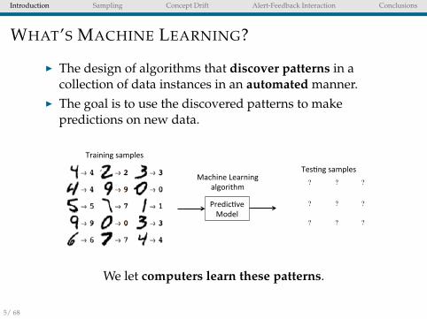
WHAT’S MACHINE LEARNING?
I The design of algorithms that discover patterns in acollection of data instances in an automated manner.
I The goal is to use the discovered patterns to makepredictions on new data.
Predic've)Model)
Training)samples)
Tes'ng)samples)Machine)Learning)
algorithm)
We let computers learn these patterns.
5/ 68

Introduction Sampling Concept Drift Alert-Feedback Interaction Conclusions
CHALLENGES FOR A DATA-DRIVEN FDS1. Unbalanced distribution (few frauds).2. Concept Drift (CD) due to fraud evolution and change in
customer behaviour.3. Few recent supervised transactions (true class of only
transactions reviewed by investigators).4. For confidentiality reason, exchange of datasets and
information is often difficult.
6/ 68

Introduction Sampling Concept Drift Alert-Feedback Interaction Conclusions
PCA PROJECTION
Figure : Transactions distribution over the first two PrincipalComponents in different days.
7/ 68

Introduction Sampling Concept Drift Alert-Feedback Interaction Conclusions
RESAMPLING METHODS
Undersampling- Oversampling- SMOTE-
Figure : Resampling methods for unbalanced classification. Thepositive and negative symbols denote fraudulent and genuinetransactions. In red the new observations created with oversamplingmethods.
8/ 68

Introduction Sampling Concept Drift Alert-Feedback Interaction Conclusions
CONCEPT DRIFTIn data streams the concept to learn can change due tonon-stationary distributions.
t +1
t
Class%priors%change% Within%class%change% Class%boundary%change%
Figure : Illustrative example of different types of Concept Drifts.
9/ 68

Introduction Sampling Concept Drift Alert-Feedback Interaction Conclusions
THESIS CONTRIBUTIONS
1. Learning with unbalanced distribution:I impact of undersampling on the accuracy of the final
classifierI racing algorithm to adaptively select the best unbalanced
strategy2. Learning from evolving and unbalanced data streams
I multiple strategies for unbalanced data stream.I effective solution to avoid propagation of old transactions.
3. Prototype of a real-world FDSI realistic framework that uses all supervised information
and provides accurate alerts.4. Software and Credit Card Fraud Detection Dataset
I release of a software package and a real-world dataset.
10/ 68

Introduction Sampling Concept Drift Alert-Feedback Interaction Conclusions
PUBLICATIONS
I A. Dal Pozzolo, G. Boracchi, O. Caelen, C. Alippi, and G. Bontempi.Credit Card Fraud Detection with Alert-Feedback Interaction.Submitted to IEEE TNNLS, 2015.
I A. Dal Pozzolo, O. Caelen, and G. Bontempi.When is undersampling effective in unbalanced classification tasks?In ECML-KDD, 2015.
I A. Dal Pozzolo, O. Caelen, R. Johnson and G. Bontempi.Calibrating Probability with Undersampling for Unbalanced Classification.In IEEE CIDM, 2015.
I A. Dal Pozzolo, G. Boracchi, O. Caelen, C. Alippi, and G. Bontempi.Credit Card Fraud Detection and Concept-Drift Adaptation with Delayed Supervised Information.In IEEE IJCNN, 2015.
I A. Dal Pozzolo, R. Johnson, O. Caelen, S. Waterschoot, N. Chawla, and G. Bontempi.Using HDDT to avoid instances propagation in unbalanced and evolving data streams.In IEEE IJCNN, 2014.
I A. Dal Pozzolo, O. Caelen, Y. Le Borgne, S. Waterschoot, and G. Bontempi.Learned lessons in credit card fraud detection from a practitioner perspective.Elsevier ESWA, 2014.
I A. Dal Pozzolo, O. Caelen, S. Waterschoot, G. Bontempi,Racing for unbalanced methods selection.In IEEE IDEAL, 2013
11/ 68

Introduction Sampling Concept Drift Alert-Feedback Interaction Conclusions
THE FRAUD DETECTION PROBLEM
I We formalize FD as a classification task f : Rn → {+,−}.I X ∈ Rn is the input and Y ∈ {+,−} the output domain.I + is the fraud (minority) and − the genuine (majority)
class.I Given a classifier K and a training set TN, we are interested
in estimating for a new sample (x, y) the posteriorprobability P(y = +|x).
Fraud&
Genuine&
12/ 68
Introduction Sampling Concept Drift Alert-Feedback Interaction Conclusions
THE FRAUD DETECTION DATA
I WL is processing millions of transactions per day.I When a transaction arrives it contains about 20 raw
features (e.g. CARD ID, AMOUNT, DATETIME,SHOP ID, CURRENCY, etc.).
I Aggregate features are compute to include the cardholderhistorical behaviour (e.g. AVG AMOUNT WEEK,TIME FROM LAST TRX, NB TRX SAME SHOP, etc.).
I Final feature vector contains about 50 variables.
13/ 68

Introduction Sampling Concept Drift Alert-Feedback Interaction Conclusions
ACCURACY MEASURE OF A FDS
I In a detection problem it is more important toprovide accurate ranking than correctclassification.
I In a realistic FDS, investigators check only alimited number of transactions.
I Hence, Pk is the most relevant measure, with kbeing the number of transactions checked.
I Pk is the proportion of frauds in k most riskytransactions.
k Predicted))Score True)Class1 0.99 +2 0.98 +3 0.98 :4 0.96 :5 0.95 +6 0.92 :7 0.91 +8 0.84 :9 0.82 :10 0.79 :11 0.76 :12 0.75 +13 0.7 :14 0.67 :15 0.64 +16 0.61 :17 0.58 :18 0.55 +19 0.52 :20 0.49 :
14/ 68

Introduction Sampling Concept Drift Alert-Feedback Interaction Conclusions
Theoretical contribution
CHAPTER 4-
UNDERSTANDING SAMPLING METHODS
Publications:I A. Dal Pozzolo, O. Caelen, and G. Bontempi.
When is undersampling effective in unbalanced classification tasks?In ECML-KDD, 2015.
I A. Dal Pozzolo, O. Caelen, R. Johnson and G. Bontempi.Calibrating Probability with Undersampling for Unbalanced Classification.In IEEE CIDM, 2015.
I A. Dal Pozzolo, O. Caelen, S. Waterschoot, G. Bontempi,Racing for unbalanced methods selection.In IEEE IDEAL, 2013
15/ 68

Introduction Sampling Concept Drift Alert-Feedback Interaction Conclusions
OBJECTIVE OF CHAPTER 4
In Chapter 4 we aim toI analyse the shift in the posterior distribution due to
undersampling and to study its impact on the finalranking.
I show under which condition undersampling is expected toimprove classification accuracy.
I propose a method to calibrate posterior probabilities andto select the classification threshold.
I show how to efficiently select the best unbalanced strategyfor a given dataset.
16/ 68

Introduction Sampling Concept Drift Alert-Feedback Interaction Conclusions
EFFECT OF UNDERSAMPLINGI Suppose that a classifier K is trained on set TN which is
unbalanced.I Let s be a random variable associated to each sample
(x, y) ∈ TN, s = 1 if the point is sampled and s = 0otherwise.
I Assume that s is independent of the input x given the classy (class-dependent selection):
P(s|y, x) = P(s|y)⇔ P(x|y, s) = P(x|y)
.
Undersampling--
Unbalanced- Balanced-
Figure : Undersampling: remove randomly majority class examples.In red samples that are removed from the unbalanced dataset (s = 0).
17/ 68
Introduction Sampling Concept Drift Alert-Feedback Interaction Conclusions
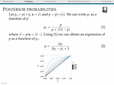
POSTERIOR PROBABILITIESLet ps = p(+|x, s = 1) and p = p(+|x). We can write ps as afunction of p:
ps =p
p + β(1− p)(1)
where β = p(s = 1|−). Using (1) we can obtain an expression ofp as a function of ps:
p =βps
βps − ps + 1(2)
Figure : p and ps at different β. Low values of β leads to a morebalanced problem.
18/ 68

Introduction Sampling Concept Drift Alert-Feedback Interaction Conclusions
SHIFT AND CLASS SEPARABILITY
(a) ps as a function of β
3 15
0
500
1000
1500
−10 0 10 20 −10 0 10 20x
Cou
nt class01
(b) Class distribution
Figure : Class distribution and posterior probability as a function of βfor two univariate binary classification tasks with norm classconditional densities X− ∼ N (0, σ) and X+ ∼ N (µ, σ) (on the leftµ = 3 and on the right µ = 15, in both examples σ = 3). Note that pcorresponds to β = 1 and ps to β < 1.
19/ 68

Introduction Sampling Concept Drift Alert-Feedback Interaction Conclusions
CONDITION FOR A BETTER RANKING
Using νs > ν and by making a hypothesis of normality in theerrors, K has better ranking with undersampling when
dps
dp>
√νs
ν(3)
where dpsdp is the derivative of ps w.r.t. p:
dps
dp=
β
(p + β(1− p))2
20/ 68

Introduction Sampling Concept Drift Alert-Feedback Interaction Conclusions
UNIVARIATE SYNTHETIC DATASET
−2 −1 0 1 2
0.0
0.2
0.4
0.6
0.8
1.0
1.2
x
Post
erio
r pro
babi
lity
(a) Class conditional distributions(thin lines) and the posterior distri-bution of the minority class (thickerline).
(b) dpsdp (solid lines),
√νsν
(dottedlines).
Figure : Non separable case. On the right we plot both terms ofinequality 3 (solid: left-hand, dotted: right-hand term) for β = 0.1and β = 0.4
21/ 68
Introduction Sampling Concept Drift Alert-Feedback Interaction Conclusions
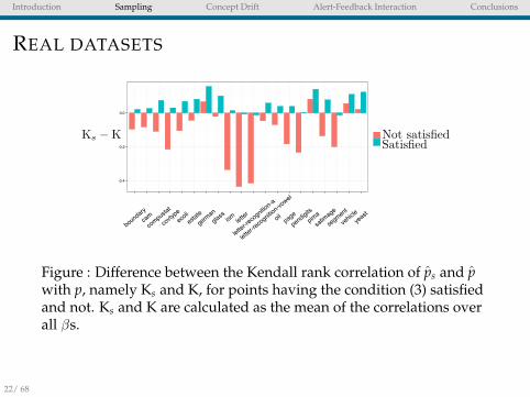
REAL DATASETS
Figure : Difference between the Kendall rank correlation of ps and pwith p, namely Ks and K, for points having the condition (3) satisfiedand not. Ks and K are calculated as the mean of the correlations overall βs.
22/ 68

Introduction Sampling Concept Drift Alert-Feedback Interaction Conclusions
REAL DATASETS II
Figure : Ratio between the number of sample satisfying condition 3and all the instances available in each dataset averaged over all theβs.
23/ 68

Introduction Sampling Concept Drift Alert-Feedback Interaction Conclusions
DISCUSSION
I When (3) is satisfied the posterior probability obtainedafter sampling returns a more accurate ordering.
I Several factors influence (3) (e.g. β, variance of theclassifier, class separability)
I Practical use (3) is not straightforward since it requiresknowledge of p and νs
ν (not easy to estimate).I The sampling rate should be tuned, using a balanced
distribution is not always the best option.
24/ 68

Introduction Sampling Concept Drift Alert-Feedback Interaction Conclusions
SELECTING THE BEST STRATEGY
I With no prior information about the data distribution isdifficult to decide which unbalanced strategy to use.
I No-free-lunch theorem [23]: no single strategy is coherentlysuperior to all others in all conditions (i.e. algorithm,dataset and performance metric)
I Testing all unbalanced techniques is not an option becauseof the associated computational cost.
I We proposed to use the Racing approach [17] to performstrategy selection.
25/ 68

Introduction Sampling Concept Drift Alert-Feedback Interaction Conclusions
RACING FOR STRATEGY SELECTION
I Racing consists in testing in parallel a set of alternativesand using a statistical test to remove an alternative if it issignificantly worse than the others.
I We adopted F-Race version [4] to search efficiently for thebest strategy for unbalanced data.
I The F-race combines the Friedman test with HoeffdingRaces [17].
26/ 68

Introduction Sampling Concept Drift Alert-Feedback Interaction Conclusions
RACING FOR UNBALANCED TECHNIQUE SELECTION
Automatically select the most adequate technique for a givendataset.
1. Test in parallel a set of alternative balancing strategies on asubset of the dataset
2. Remove progressively the alternatives which aresignificantly worse.
3. Iterate the testing and removal step until there is only onecandidate left or not more data is available
Candidate(1 Candidate(2 Candidate(3subset(1( 0.50 0.47 0.48subset(2 0.51 0.48 0.30subset(3 0.51 0.47subset(4 0.60 0.45subset(5 0.55
Candidate(1 Candidate(2 Candidate(3subset(1( 0.50 0.47 0.48subset(2 0.51 0.48 0.30subset(3 0.51 0.47subset(4 0.49 0.46subset(5 0.48 0.46subset(6 0.60 0.45subset(7 0.59subset(8subset(9subset(10
Original(Dataset
Time
27/ 68
Introduction Sampling Concept Drift Alert-Feedback Interaction Conclusions
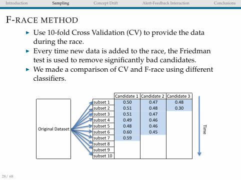
F-RACE METHODI Use 10-fold Cross Validation (CV) to provide the data
during the race.I Every time new data is added to the race, the Friedman
test is used to remove significantly bad candidates.I We made a comparison of CV and F-race using different
classifiers.
Candidate(1 Candidate(2 Candidate(3subset(1( 0.50 0.47 0.48subset(2 0.51 0.48 0.30subset(3 0.51 0.47subset(4 0.60 0.45subset(5 0.55
Candidate(1 Candidate(2 Candidate(3subset(1( 0.50 0.47 0.48subset(2 0.51 0.48 0.30subset(3 0.51 0.47subset(4 0.49 0.46subset(5 0.48 0.46subset(6 0.60 0.45subset(7 0.59subset(8subset(9subset(10
Original(Dataset
Time
28/ 68

Introduction Sampling Concept Drift Alert-Feedback Interaction Conclusions
F-RACE VS CROSS VALIDATIONDataset Exploration Method Ntest % Gain Mean Sd
ecoliRace Under 46 49 0.836 0.04CV SMOTE 90 - 0.754 0.112
letter-aRace Under 34 62 0.952 0.008CV SMOTE 90 - 0.949 0.01
letter-vowelRace Under 34 62 0.884 0.011CV Under 90 - 0.887 0.009
letterRace SMOTE 37 59 0.951 0.009CV Under 90 - 0.951 0.01
oilRace Under 41 54 0.629 0.074CV SMOTE 90 - 0.597 0.076
pageRace SMOTE 45 50 0.919 0.01CV SMOTE 90 - 0.92 0.008
pendigitsRace Under 39 57 0.978 0.011CV Under 90 - 0.981 0.006
PhosSRace Under 19 79 0.598 0.01CV Under 90 - 0.608 0.016
satimageRace Under 34 62 0.843 0.008CV Under 90 - 0.841 0.011
segmentRace SMOTE 90 0 0.978 0.01CV SMOTE 90 - 0.978 0.01
estateRace Under 27 70 0.553 0.023CV Under 90 - 0.563 0.021
covtypeRace Under 42 53 0.924 0.007CV SMOTE 90 - 0.921 0.008
camRace Under 34 62 0.68 0.007CV Under 90 - 0.674 0.015
compustatRace Under 37 59 0.738 0.021CV Under 90 - 0.745 0.017
creditcardRace Under 43 52 0.927 0.008CV SMOTE 90 - 0.924 0.006
Table : Results in terms of G-mean for RF classifier.29/ 68

Introduction Sampling Concept Drift Alert-Feedback Interaction Conclusions
DISCUSSION
I The best strategy is extremely dependent on the datanature, algorithm adopted and performance measure.
I F-race is able to automatise the selection of the bestunbalanced strategy for a given unbalanced problemwithout exploring the whole dataset.
I For the fraud dataset the unbalanced strategy chosen had abig impact on the accuracy of the results.
30/ 68

Introduction Sampling Concept Drift Alert-Feedback Interaction Conclusions
CONCLUSIONS OF CHAPTER 4
I Undersampling is not always the best strategy for allunbalanced datasets.
I This result warning against a naive use of undersamplingin unbalanced tasks.
I With racing [9] we can rapidly select the best strategy for agiven unbalanced task.
I However, we see that undersampling and SMOTE areoften the best strategy to adopt for FD.
31/ 68

Introduction Sampling Concept Drift Alert-Feedback Interaction Conclusions
Methodologicalcontribution
CHAPTER 5-
LEARNING WITH CONCEPT DRIFT
Publications:I A. Dal Pozzolo, O. Caelen, Y. Le Borgne, S. Waterschoot, and G. Bontempi.
Learned lessons in credit card fraud detection from a practitioner perspective.Elsevier ESWA, 2014.
I A. Dal Pozzolo, R. Johnson, O. Caelen, S. Waterschoot, N. Chawla, and G. Bontempi.Using HDDT to avoid instances propagation in unbalanced and evolving data streams.In IEEE IJCNN, 2014.
32/ 68

Introduction Sampling Concept Drift Alert-Feedback Interaction Conclusions
OBJECTIVE OF CHAPTER 5
The objectives of this chapter are:I investigating the benefit of updating the FDS.I assessing the impact of Concept Drift (CD).I comparing alternative learning strategies for CD.I studying an effective way to deal with unbalanced
distribution in a streaming environment.
33/ 68

Introduction Sampling Concept Drift Alert-Feedback Interaction Conclusions
LEARNING APPROACHES
We compare three standard learning approaches ontransactions from February 2012 to May 2013.
Approach Strengths WeaknessesStatic • Speed • No CD adaptation
Update • No instances propagation • Need several batches• CD adaptation for the minority class
Propagate and Forget • Accumulates minority • Propagation leads toinstances faster larger training time
• CD adaptation
# Days # Features # Transactions Period422 45 2’202’228 1Feb12 - 20May13
34/ 68

Introduction Sampling Concept Drift Alert-Feedback Interaction Conclusions
THE STATIC APPROACH
Time%Sta)c%approach%
Fraudulent%transac)ons%Genuine%transac)ons%
Bt�2 Bt�1 Bt Bt+1 Bt+2 Bt+3 Bt+4
Mt
35/ 68

Introduction Sampling Concept Drift Alert-Feedback Interaction Conclusions
THE UPDATE APPROACH
Time%Update%approach%
Bt�2 Bt�1 Bt Bt+1
Mt�2 Mt�1 MtMt�3
Et
Bt�5 Bt�4 Bt�3
Fraudulent%transac)ons%Genuine%transac)ons%
36/ 68

Introduction Sampling Concept Drift Alert-Feedback Interaction Conclusions
THE PROPAGATE AND FORGET APPROACH
Time%Propagate%and%Forget%approach%
Bt�2 Bt�1 Bt Bt+1Bt�3
Mt�2 Mt�1 MtMt�3
EtFraudulent%transac)ons%Genuine%transac)ons%
37/ 68

Introduction Sampling Concept Drift Alert-Feedback Interaction Conclusions
BEST OVERALL STRATEGYThe Propagate and Forget approach is the best while the Staticapproach is the worst.
NNET.Under.One.1M.Static.60KSVM.Under.One.1M.Static.60K
NNET.Under.One.1M.Static.90KSVM.Under.One.1M.Static.90K
NNET.Under.One.1M.Static.120KSVM.Under.One.1M.Static.120K
RF.Under.One.1M.Static.30KRF.Under.One.1M.Static.60K
RF.SMOTE.One.1M.Static.90KRF.Under.One.1M.Static.90K
RF.EasyEnsemble.One.1M.Static.90KRF.Under.One.1M.Static.120K
RF.Under.15days.1M.Update.90KRF.Under.Daily.30M.Forget.30Kgen
RF.Under.Weekly.1M.Update.90KRF.Under.Daily.15M.Forget.30KgenRF.Under.Daily.10M.Forget.30Kgen
RF.Under.Daily.1M.Update.90KRF.Under.Daily.30M.Update.90K
RF.SMOTE.Daily.1M.Forget.90KgenRF.Under.Daily.5M.Forget.30KgenRF.Under.Daily.1M.Forget.90Kgen
RF.Under.Daily.15M.Update.90KRF.Under.Daily.5M.Update.90K
RF.EasyEnsemble.Daily.1M.Update.90KRF.SMOTE.Daily.1M.Update.90K
RF.EasyEnsemble.Daily.1M.Forget.90Kgen
0 1000 2000 3000 4000
Sum of the ranks
Best significantFALSETRUE
Metric: PrecisionRank
Figure : Comparison of all strategies using sum of ranks in all batcheswhen using Pk as accuracy measure.
38/ 68

Introduction Sampling Concept Drift Alert-Feedback Interaction Conclusions
DISCUSSION
I Without CD we would expect the three approaches toperform similarly.
I The static approach is consistently the worst.I Ensembles are often better alternative than single models.I Higher accuracy can be achieved by using SMOTE or
undersampling the data.I Instance propagation can be an alternative way to
rebalance the data stream.
39/ 68

Introduction Sampling Concept Drift Alert-Feedback Interaction Conclusions
CONCLUSION OF CHAPTER 5
I Updating the models daily and combining them intoensemble is an effective strategy to adapt to CD.
I Retaining positives samples/undersampling the datastream improves the accuracy of the FDS.
I However, it is not always possible to either revisit or storeold instances of a data stream.
I In that case we reccomend using Hellinger DistanceDecision Tree [7] (HDDT) to avoid instances propagation.
40/ 68

Introduction Sampling Concept Drift Alert-Feedback Interaction Conclusions
Proposed FDS
CHAPTER 6-
LEARNING WITH ALERT-FEEDBACK INTERACTION
Publications:I A. Dal Pozzolo, G. Boracchi, O. Caelen, C. Alippi, and G. Bontempi.
Credit Card Fraud Detection with Alert-Feedback Interaction.Submitted to IEEE TNNLS, 2015.
I A. Dal Pozzolo, G. Boracchi, O. Caelen, C. Alippi, and G. Bontempi.Credit Card Fraud Detection and Concept-Drift Adaptation with Delayed Supervised Information.In IEEE IJCNN, 2015.
41/ 68
Introduction Sampling Concept Drift Alert-Feedback Interaction Conclusions
OBJECTIVE OF CHAPTER 6
I Propose a framework meeting realistic working conditions.I Model the interaction between the FDS generating alerts
and investigators.I Integrate investigators’ feedback in the FDS.
42/ 68
Introduction Sampling Concept Drift Alert-Feedback Interaction Conclusions
REALISTIC WORKING CONDITIONS
I Alert-Feedback Interaction: the supervised samplesdepends on the alerts reported to investigators.
I Only a small set of alerts can be checked by humaninvestigators.
I The labels of the majority of transactions are available onlyseveral days later (after customers have reportedunauthorized transactions).
I Investigators trust a FDS only if it provides accurate alerts,i.e. alert precision (Pk) is the accuracy measure thatmatters.
43/ 68

Introduction Sampling Concept Drift Alert-Feedback Interaction Conclusions
SUPERVISED SAMPLES
I The k transactions with largest PKt−1(+|x) define the alertsAt reported to the investigators.
I Investigators provide a feedback about the alerts in At,defining a set of k supervised couples (x, y):
Ft = {(x, y), x ∈ At}, (4)
I Ft are the only immediate supervised samples.I Dt−δ are transactions that have not been checked by
investigators, but their label is assumed to be correct afterthat δ days have elapsed.
44/ 68

Introduction Sampling Concept Drift Alert-Feedback Interaction Conclusions
SUPERVISED SAMPLES III Ft are a small set of risky transactions according the FDS.I Dt−δ contains all the occurred transactions in a day (≈ 99%
genuine transactions).
t −1 t t +1
Feedbacks)Delayed)Samples)
t −δ
All)fraudulent)transac6ons)of)a)day)
All)genuine)transac6ons)of)a)day)
Fraudulent)transac6ons)in)the)feedback)Genuine)transac6ons)in)the)feedback)
FtFt�1Ft�3Ft�4Ft�5Ft�6 Ft�2Dt�7Dt�8 Bt+1
Figure : The supervised samples available at day t include: i)feedbacks of the first δ days and ii) delayed couples occurred beforethe δth day.
45/ 68
Introduction Sampling Concept Drift Alert-Feedback Interaction Conclusions
FEEDBACKS VS DELAYED SAMPLES
Learning from feedbacks Ft is a different problem than learningfrom delayed samples in Dt−δ:
I Ft provides recent, up-to-date, information while Dt−δmight be already obsolete once it comes.
I Percentage of frauds in Ft and Dt−δ is different.I Samples in Ft are selected as the most risky by Kt−1.I A classifier trained on Ft learns how to label transactions
that are most likely to be fraudulent.
Feedbacks and delayed samples have to be treated separately.
46/ 68

Introduction Sampling Concept Drift Alert-Feedback Interaction Conclusions
LEARNING STRATEGYA conventional solution for CD adaptation isWt [20]. To learnseparately from feedbacks and delayed transactions wepropose AW
t (aggregation of Ft andWDt ).
FtFt�1Ft�3Ft�4Ft�5Ft�6 Ft�2Dt�7Dt�8
Wt
FtWDt
AWt
Figure : Learning strategies for feedbacks and delayed transactionsoccurring in the two days (M = 2) before the feedbacks (δ = 7).
47/ 68

Introduction Sampling Concept Drift Alert-Feedback Interaction Conclusions
CLASSIFIER AGGREGATIONS
WDt has to be aggregated with Ft to exploit information
provided by feedbacks. We combine these classifiers byaveraging the posterior probabilities.
PAWt
(+|x) = αtPFt(+|x) + (1− αt)PWDt
(+|x) (5)
AWt with αt ≥ 0.5 gives larger influence to feedbacks on the
probability estimates w.r.tWt.
48/ 68

Introduction Sampling Concept Drift Alert-Feedback Interaction Conclusions
DATASETSWe used three datasets of e-commerce credit card transactions(fraud << 1%):
Table : Datasets
Id Start day End day # Days # Transactions # Features2013 2013-09-05 2014-01-18 136 21’830’330 512014 2014-08-05 2014-12-31 148 27’113’187 512015 2015-01-05 2015-05-31 146 27’651’197 51
2013 2014 2015
●
●●●●
●●
●
●●●●
●
●●●
●
●
●
●●●
●
●
●●
●
●
●
●●●
●
●
●
●
●
●●●●●●●
●●●
●
●
●
●●
●
●
●
●●
●●
●●
●
●●
●●
●
●●
●●●
●
●
●
●
●
●●●
●
●●●●●
●
●●●
●●
●●●●
●●
●
●
●
●
●●●●
●●●●●●●●●●●
●●●●●●●●
●●●
●
●
●●●●●
●
●
●
●●●●
●●
●●
●
●
●
●
●●
●
●
●●
●
●
●●
●
●
●●●
●●
●●
●●
●
●
●●●
●
●●
●
●●●●●
●●●
●●
●●
●
●●●●
●●
●
●
●●●●
●●
●●●
●
●●●●●●●●●●●●
●
●
●
●
●
●●
●●●
●
●
●
●●
●
●●
●
●
●
●●●●
●
●
●
●
●
●
●
●
●
●●●
●●●
●
●●
●
●●
●●●●●
●●●●●●●
●●
●●
●●●
●
●
●
●
●
●
●
●●
●●
●●●●●
●
●●
●●
●
●
●
●
●
●
●
●
●
●
●
●●
●●●●
●
●
●●●●●●●
●
●●
●
●●
●
●●●
●
●
●
●●
●
●
●
●●
●
●●
●
●
●●
●
●●●●●
●
●●
●●●●
●
●
●●●
●
●●●
●●
●
●
●
●●
●
●
●●●●●
●●●
●
●
●●
●●●
●
●
●
●
●
●●
●●●
●
●
●●●
●
●●●●
●
0
500
1000
1500
2000
2500
Sep Oct Nov Dec Jan Aug Sep Oct Nov Dec JanJan Feb Mar Apr May Jun
Day
Num
ber
of fr
auds
49/ 68

Introduction Sampling Concept Drift Alert-Feedback Interaction Conclusions
SEPARATING FEEDBACKS FROM DELAYED SAMPLESAggregating two distinct classifiers (Ft withWD
t ) using AWt is
better than pooling together feedbacks and delayed sampleswithWt.
dataset classifier mean sd2013 F 0.62 0.252013 WD 0.54 0.222013 W 0.57 0.232013 AW 0.70 0.212014 F 0.59 0.292014 WD 0.58 0.262014 W 0.60 0.262014 AW 0.69 0.242015 F 0.67 0.252015 WD 0.66 0.212015 W 0.68 0.212015 AW 0.75 0.20
Table : Average Pk with δ = 7, M = 16 and αt = 0.5.
50/ 68

Introduction Sampling Concept Drift Alert-Feedback Interaction Conclusions
EXPERIMENTS WITH ARTIFICIAL CD
AW
W
(a) Sliding window strate-gies on dataset CD1
AW
W
(b) Sliding window strate-gies on dataset CD2
WAW
(c) Sliding window strate-gies on dataset CD3
Figure : Average Pk per day on datasets with artificial CD usingmoving average of 15 days. The vertical bar denotes the date of CD.
51/ 68

Introduction Sampling Concept Drift Alert-Feedback Interaction Conclusions
CLASSIFIERS IGNORING AFIExperiments with a classifierRt trained on all recenttransactions between t and t− δ. Rt makes the unrealisticassumption that all transactions are labeled by investigators.
FtFt�1Ft�3Ft�4Ft�5Ft�6 Ft�2Dt�7Dt�8
FtWDt
AWt
Rt
Figure : Rt makes the unrealistic assumption that all transactionsbetween t and t− δ have been checked by investigators.
52/ 68

Introduction Sampling Concept Drift Alert-Feedback Interaction Conclusions
CLASSIFIERS IGNORING AFI II
AUC is a global ranking measure, while Pk measures theranking quality only on the top k.
(a) dataset 2013metric classifier mean sdAUC F 0.83 0.06AUC WD 0.94 0.03AUC R 0.96 0.01AUC AW 0.94 0.03
Pk F 0.67 0.24Pk WD 0.54 0.22Pk R 0.60 0.22Pk AW 0.72 0.20
(b) dataset 2014metric classifier mean sdAUC F 0.81 0.08AUC WD 0.94 0.03AUC R 0.96 0.02AUC AW 0.93 0.03
Pk F 0.67 0.27Pk WD 0.56 0.27Pk R 0.63 0.25Pk AW 0.71 0.25
(c) dataset 2015metric classifier mean sdAUC F 0.81 0.07AUC WD 0.95 0.02AUC R 0.97 0.01AUC AW 0.94 0.02
Pk F 0.71 0.21Pk WD 0.62 0.21Pk R 0.68 0.20Pk AW 0.76 0.19
Table : Average AUC and Pk for the sliding approach (δ = 15, M = 16and αt = 0.5).
53/ 68

Introduction Sampling Concept Drift Alert-Feedback Interaction Conclusions
ADAPTIVE WEIGHTING
Experiments with different weighting strategies in AWt .
(a) dataset 2013α adaptation mean sdprobDif 0.70 0.22acc 0.72 0.21accMiss 0.72 0.21precision 0.72 0.21recall 0.71 0.21auc 0.72 0.21none(αt = 0.5) 0.72 0.20
(b) dataset 2014α adaptation mean sdprobDif 0.68 0.26acc 0.71 0.24accMiss 0.70 0.24precision 0.71 0.24recall 0.70 0.25auc 0.71 0.24none(αt = 0.5) 0.71 0.24
(c) dataset 2015α adaptation mean sdprobDif 0.73 0.21acc 0.76 0.19accMiss 0.75 0.19precision 0.75 0.19recall 0.74 0.20auc 0.75 0.19none(αt = 0.5) 0.76 0.19
Table : Average Pk of AWt with adaptive αt (δ = 15).
54/ 68
Introduction Sampling Concept Drift Alert-Feedback Interaction Conclusions
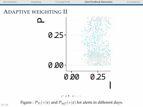
ADAPTIVE WEIGHTING II
Figure : PFt(+|x) and PWDt(+|x) for alerts in different days.
55/ 68

Introduction Sampling Concept Drift Alert-Feedback Interaction Conclusions
CONCLUSION OF CHAPTER 6
I The goal of the FDS is to return precise alerts (high Pk).I In a realistic settings feedbacks and delayed samples are
the only supervised information available.I Feedbacks and delayed samples address two different
classification tasks.I Not convenient to pool the two types of supervised
samples together.
56/ 68

Introduction Sampling Concept Drift Alert-Feedback Interaction Conclusions
CONCLUSIONS ANDFUTURE PERSPECTIVES
57/ 68

Introduction Sampling Concept Drift Alert-Feedback Interaction Conclusions
SUMMARY OF CONTRIBUTIONS
In this thesis we:I formalize realistic working conditions of a FDS.I study how undersampling can improve the ranking of a
classifier K.I release a R package called unbalanced [8] with racing.I investigate strategies for data streams with both CD and
unbalanced distribution.I prototype a real-world FDS that, for the first time, learns
from investigators’ feedback and allows us to have moreprecise alerts.
58/ 68

Introduction Sampling Concept Drift Alert-Feedback Interaction Conclusions
LEARNED LESSONS
I Rebalancing a training set with undersampling is notguaranteed to improve performances.
I F-Race [4] can be effective to rapidly select the unbalancedtechnique to use.
I The data stream defined by credit card transactions isseverely affected by CD, updating the FDS is often a goodidea.
I For a real-world FDS it is mandatory to produce precisealerts.
I Feedbacks and delayed samples should be separatelyhandled when training a FDS.
I Aggregating two distinct classifiers is an effective strategyand that it enables a quicker adaptation to CD.
59/ 68

Introduction Sampling Concept Drift Alert-Feedback Interaction Conclusions
TAKE-HOME MESSAGES
I Class imbalance and CD seriously affect the performancesof a classifier.
I In a real-world scenario, there is a strong Alert-Feedbackinteraction that has to be explicitly considered.
I The best learning algorithm for a FDS changes with theaccuracy measure.
I A standard classifier that is trained on all recenttransactions is not the best when we want to produceaccurate alerts.
60/ 68

Introduction Sampling Concept Drift Alert-Feedback Interaction Conclusions
FUTURE WORK: TOWARDS BIG DATA SOLUTIONS
I This work will be continued in the BruFence project.I Big Data Mining for Fraud Detection and Security.I Three research groups (ULB-QualSec, ULB-MLG and
UCL-MLG) and three companies (Worldline, Steria andNviso).
I 2015 - 2018 funded by InnovIRIS (Brussels Region).
BruFence&
• Big&Data&Mining&for&Fraud&Detec;on&and&Security&&• 2015O2018&funded&by&Innoviris&(Brussels&Region).&&
• ULB - QualSec
• ULB - MLG
• UCL - MLG
!
!
!
!
• Wordline
• Steria
• NViso
BruFence - consortium
Spice
• ULB - QualSec
• ULB - MLG
• UCL - MLG
!
!
!
!
• Wordline
• Steria
• NViso
BruFence - consortium
Spice
• ULB - QualSec
• ULB - MLG
• UCL - MLG
!
!
!
!
• Wordline
• Steria
• NViso
BruFence - consortium
Spice
• ULB - QualSec
• ULB - MLG
• UCL - MLG
!
!
!
!
• Wordline
• Steria
• NViso
BruFence - consortium
Spice
61/ 68

Introduction Sampling Concept Drift Alert-Feedback Interaction Conclusions
THE BruFence PROJECT
I Goal: implement the FDS of Chapter 6 using Big Datatechnologies (e.g. Spark, NoSQL DB).
I Real-time framework scalable w.r.t. the amount of dataand resources available.
I Determine to which extent external network data canimprove prediction accuracy.
I Compute aggregated features in real time and using alarger set of historical transactions.
Figure : Apache Big Data softwares
62/ 68

Introduction Sampling Concept Drift Alert-Feedback Interaction Conclusions
ADDED VALUE FOR WL
I RF has emerged as the best algorithm (now used by WL).I New ways to create aggregated features.I Undersampling can be used to improve the accuracy of
FDS, but probabilities need to be calibrated.I Our experimental analysis on CD gave WL some
guidelines on how to improve the FDS.I Including feedbacks in the learning process allows WL to
obtain more accurate alerts.
63/ 68

Introduction Sampling Concept Drift Alert-Feedback Interaction Conclusions
CONCLUDING REMARKS
I Doctiris was an unique opportunity to work on real-worldfraud detection data.
I Real working conditions define new challenges (oftenignored in the literature).
I Companies are more interested on practical results, whileacademics on theoretical ones.
I Industry and university, should look at each other andexchange ideas in order to have a much larger impact onsociety.
64/ 68

Introduction Sampling Concept Drift Alert-Feedback Interaction Conclusions
Website: www.ulb.ac.be/di/map/adalpozzEmail: [email protected]
Thank you for the attention
65/ 68

Introduction Sampling Concept Drift Alert-Feedback Interaction Conclusions
BIBLIOGRAPHY I[1] D. N. A. Asuncion.
UCI machine learning repository, 2007.
[2] C. Alippi, G. Boracchi, and M. Roveri.A just-in-time adaptive classification system based on the intersection of confidence intervals rule.Neural Networks, 24(8):791–800, 2011.
[3] A. Bifet, G. Holmes, R. Kirkby, and B. Pfahringer.Moa: Massive online analysis.The Journal of Machine Learning Research, 99:1601–1604, 2010.
[4] M. Birattari, T. Stutzle, L. Paquete, and K. Varrentrapp.A racing algorithm for configuring metaheuristics.In Proceedings of the genetic and evolutionary computation conference, pages 11–18, 2002.
[5] D. A. Cieslak and N. V. Chawla.Detecting fractures in classifier performance.In Data Mining, 2007. ICDM 2007. Seventh IEEE International Conference on, pages 123–132. IEEE, 2007.
[6] D. A. Cieslak and N. V. Chawla.Learning decision trees for unbalanced data.In Machine Learning and Knowledge Discovery in Databases, pages 241–256. Springer, 2008.
[7] D. A. Cieslak, T. R. Hoens, N. V. Chawla, and W. P. Kegelmeyer.Hellinger distance decision trees are robust and skew-insensitive.Data Mining and Knowledge Discovery, 24(1):136–158, 2012.
[8] A. Dal Pozzolo, O. Caelen, and G. Bontempi.unbalanced: Racing For Unbalanced Methods Selection., 2015.R package version 2.0.
65/ 68

Introduction Sampling Concept Drift Alert-Feedback Interaction Conclusions
BIBLIOGRAPHY II[9] A. Dal Pozzolo, O. Caelen, S. Waterschoot, and G. Bontempi.
Racing for unbalanced methods selection.In Proceedings of the 14th International Conference on Intelligent Data Engineering and Automated Learning. IDEAL,2013.
[10] C. Elkan.The foundations of cost-sensitive learning.In International Joint Conference on Artificial Intelligence, volume 17, pages 973–978. Citeseer, 2001.
[11] R. Elwell and R. Polikar.Incremental learning of concept drift in nonstationary environments.Neural Networks, IEEE Transactions on, 22(10):1517–1531, 2011.
[12] J. Gao, B. Ding, W. Fan, J. Han, and P. S. Yu.Classifying data streams with skewed class distributions and concept drifts.Internet Computing, 12(6):37–49, 2008.
[13] T. R. Hoens, R. Polikar, and N. V. Chawla.Learning from streaming data with concept drift and imbalance: an overview.Progress in Artificial Intelligence, 1(1):89–101, 2012.
[14] M. G. Kelly, D. J. Hand, and N. M. Adams.The impact of changing populations on classifier performance.In Proceedings of the fifth ACM SIGKDD international conference on Knowledge discovery and data mining, pages367–371. ACM, 1999.
[15] A. Liaw and M. Wiener.Classification and regression by randomforest.R News, 2(3):18–22, 2002.
66/ 68

Introduction Sampling Concept Drift Alert-Feedback Interaction Conclusions
BIBLIOGRAPHY III[16] R. N. Lichtenwalter and N. V. Chawla.
Adaptive methods for classification in arbitrarily imbalanced and drifting data streams.In New Frontiers in Applied Data Mining, pages 53–75. Springer, 2010.
[17] O. Maron and A. Moore.Hoeffding races: Accelerating model selection search for classification and function approximation.Robotics Institute, page 263, 1993.
[18] C. R. Rao.A review of canonical coordinates and an alternative to correspondence analysis using hellinger distance.Questiio: Quaderns d’Estadıstica, Sistemes, Informatica i Investigacio Operativa, 19(1):23–63, 1995.
[19] M. Saerens, P. Latinne, and C. Decaestecker.Adjusting the outputs of a classifier to new a priori probabilities: a simple procedure.Neural computation, 14(1):21–41, 2002.
[20] D. K. Tasoulis, N. M. Adams, and D. J. Hand.Unsupervised clustering in streaming data.In ICDM Workshops, pages 638–642, 2006.
[21] V. N. Vapnik and V. Vapnik.Statistical learning theory, volume 1.Wiley New York, 1998.
[22] S. Wang, K. Tang, and X. Yao.Diversity exploration and negative correlation learning on imbalanced data sets.In Neural Networks, 2009. IJCNN 2009. International Joint Conference on, pages 3259–3266. IEEE, 2009.
[23] D. H. Wolpert.The lack of a priori distinctions between learning algorithms.Neural computation, 8(7):1341–1390, 1996.
67/ 68

Introduction Sampling Concept Drift Alert-Feedback Interaction Conclusions
BIBLIOGRAPHY IV
68/ 68

Introduction Sampling Concept Drift Alert-Feedback Interaction Conclusions
OPEN ISSUES
I Agreeing on a good performance measure (cost-based Vsdetection).
I Modelling Alert-Feedback Interaction.I Using both the supervised and unsupervised information
available.
68/ 68

Introduction Sampling Concept Drift Alert-Feedback Interaction Conclusions
AVERAGE PRECISION
Let N+ be the number of positive (fraud) case in the originaldataset and TPk be the number of true positives in the first kranked transactions (TPk ≤ k). Let us denote Precision andRecall at k as Pk = TPk
k and Rk = TPkN+ . We can then define AP as:
AP =
N∑k=1
Pk(Rk − Rk−1) (6)
where N is the total number of observation in the dataset.
68/ 68

Introduction Sampling Concept Drift Alert-Feedback Interaction Conclusions
RANKING ERRORWe have a wrong ranking if p1 > p2 and its probability is:
P(p2 < p1) = P(p2 + ε2 < p1 + ε1) = P(ε1 − ε2 > ∆p)
where ε2 − ε1 ∼ N (0, 2ν). By making an hypothesis ofnormality we have
P(ε1 − ε2 > ∆p) = 1− Φ
(∆p√
2ν
)(7)
where Φ is the cumulative distribution function of the standardnormal distribution.The probability of a ranking error with undersampling is:
P(ps,2 < ps,1) = P(η1 − η2 > ∆ps)
and
P(η1 − η2 > ∆ps) = 1− Φ
(∆ps√
2νs
)(8)
68/ 68

Introduction Sampling Concept Drift Alert-Feedback Interaction Conclusions
CLASSIFICATION THRESHOLD
Let r+ and r− be the risk of predicting an instance as positiveand negative:
r+ = (1− p) · l1,0 + p · l1,1r− = (1− p) · l0,0 + p · l0,1
where li,j is the cost in predicting i when the true class is j andp = P(y = +|x). A sample is predicted as positive ifr+ ≤ r− [21].
Alternatively, predict as positive when p > τ with τ :
τ =l1,0 − l0,0
l1,0 − l0,0 + l0,1 − l1,1(9)
68/ 68

Introduction Sampling Concept Drift Alert-Feedback Interaction Conclusions
CONDITION FOR A BETTER RANKINGK has better ranking with undersampling w.r.t. a classifierlearned with unbalanced distribution when
P(p2 < p1) > P(ps,2 < ps,1)
P(ε1 − ε2 > ∆p) > P(η1 − η2 > ∆ps) (10)
or equivalently from (7) and (8) when
1− Φ
(∆p√
2ν
)> 1− Φ
(∆ps√
2νs
)⇔ Φ
(∆p√
2ν
)< Φ
(∆ps√
2νs
)since Φ is monotone non decreasing and νs > ν: Then it followsthat undersampling is useful (better ranking) when
dps
dp>
√νs
ν
68/ 68

Introduction Sampling Concept Drift Alert-Feedback Interaction Conclusions
CORRECTING POSTERIOR PROBABILITIES
We propose to use p′, the bias-corrected probability obtainedfrom ps:
p′ =βps
βps − ps + 1(11)
Eq. (11) is a special case of the framework proposed by Saerenset al. [19] and Elkan [10] for correcting the posterior probabilityin the case of testing and training sets sharing the same priors.
68/ 68

Introduction Sampling Concept Drift Alert-Feedback Interaction Conclusions
CORRECTING THE CLASSIFICATION THRESHOLDWhen the costs of a FN (l0,1) and FP (l1,0) are unknown, we canuse the priors. Let l1,0 = π+ and l0,1 = π−, from (9) we get:
τ =l1,0
l1,0 + l0,1=
π+
π+ + π−= π+ (12)
since π+ + π− = 1. Then we should use π+ as threshold with p:
p −→ τ = π+
Similarlyps −→ τs = π+
s
From Elkan [10]:τ ′
1− τ ′1− τs
τs= β (13)
Therefore, we obtain:
p′ −→ τ ′ = π+
68/ 68

Introduction Sampling Concept Drift Alert-Feedback Interaction Conclusions
CREDIT CARDS DATASETReal-world credit card dataset with transactions from Sep 2013,frauds account for 0.172% of all transactions.
LB RF SVM
●●●●●●●●●● ●●●●●●●●●●●●●●●●●●●● ●●●●●●●●●●
●●●●●●●●●●●●●●●●●●●● ●●●●●●●●●●●●●●●●●●●●
●●●●●● ●●●●●●
●●●●●● ●●●●●●
●●●●●● ●●●●●●
●●●●●●●● ●●●●●●●●
●●●●●●●● ●●●●●●●●
●
●
●
●
●
●
●
●
●
●
●
●
●
●
●
●
●
●
●
●
●
●
●
●
●
●
●
●
●
●
●
●
0.900
0.925
0.950
0.975
1.000
0.10.
20.
30.
40.
50.
60.
70.
80.
9 10.
10.
20.
30.
40.
50.
60.
70.
80.
9 10.
10.
20.
30.
40.
50.
60.
70.
80.
9 1
beta
AU
CProbability
pp'ps
Credit−card
LB RF SVM●●●●●●●●●●●●●●●●●●●●
●●●●●●●●●●
●●●●●●●●●●
●●●●●●
●●●●●●
●●●●●●●●●●●●
●●●●●●
●●●●●●
●●●●●●●● ●●●●●●●●
3e−04
6e−04
9e−04
0.10.
20.
30.
40.
50.
60.
70.
80.
9 10.
10.
20.
30.
40.
50.
60.
70.
80.
9 10.
10.
20.
30.
40.
50.
60.
70.
80.
9 1
beta
BS
Probabilitypp'ps
Credit−card
68/ 68

Introduction Sampling Concept Drift Alert-Feedback Interaction Conclusions
DISCUSSION
I As a result of undersampling, ps is shifted away from p.I Using (11), we can remove the drift in ps and obtain p′
which has better calibration.I p′ provides the same ranking quality of ps.I Using p′ with τ ′ we are able to improve calibration without
losing predictive accuracy.I Unfortunately there is no way to select the best β
automatically yet.
68/ 68

Introduction Sampling Concept Drift Alert-Feedback Interaction Conclusions
HELLINGER DISTANCE
I Quantify the similarity between two probabilitydistributions [18]
I Recently proposed as a splitting criteria in decision treesfor unbalanced problems [6, 7].
I In data streams, it has been used to detect classifierperformance degradation due to concept drift [5, 16].
68/ 68

Introduction Sampling Concept Drift Alert-Feedback Interaction Conclusions
HELLINGER DISTANCE II
Consider two probability measures P1,P2 of discretedistributions in Φ. The Hellinger distance is defined as:
HD(P1,P2) =
√√√√∑φ∈Φ
(√P1(φ)−
√P2(φ)
)2(14)
Hellinger distance has several properties:
I HD(P1,P2) = HD(P1,P2) (symmetric)I HD(P1,P2) >= 0 (non-negative)I HD(P1,P2) ∈ [0,
√2]
HD is close to zero when the distributions are similar and closeto√
2 for distinct distributions.
68/ 68

Introduction Sampling Concept Drift Alert-Feedback Interaction Conclusions
HELLINGER DISTANCE DECISION TREES
I HDDT [6] use Hellinger Distance as splitting criteria indecision trees for unbalanced problems.
I All numerical features are partitioned into q bins (onlycategorical variables).
I The Hellinger Distance between the positive and negativeclass is computed for each feature and then the featurewith the maximum distance is used to split the tree.
HD(f +, f−) =
√√√√√ q∑j=1
√ |f +j ||f +| −
√|f−j ||f−|
2
(15)
where j defines the jth bin of feature f and |f +j | is the number of
positive instances of feature f in the jth bin.Note that the class priors do not appear explicitly in (15).
68/ 68

Introduction Sampling Concept Drift Alert-Feedback Interaction Conclusions
AVOIDING INSTANCES PROPAGATION
I HDDT allows us to remove instance propagations betweenbatches, benefits:
I improved predictive accuracyI improved speedI single-pass through the data.
I An ensemble of HDDTs is used to adapt to CD andincrease the accuracy of single classifiers.
I We test our framework on several streaming datasets withunbalanced classes and concept drift.
68/ 68

Introduction Sampling Concept Drift Alert-Feedback Interaction Conclusions
DATASETS
We used different types of datasets.I UCI datasets [1] (unbalanced, no CD).I Synthetic datasets from MOA [3] (artificial CD).I A credit card dataset (online payment transactions
between the 5th and the 25th of Sept. 2013).
Name Source Instances Features Imbalance RatioAdult UCI 48,842 14 3.2:1
can UCI 443,872 9 52.1:1compustat UCI 13,657 20 27.5:1
covtype UCI 38,500 10 13.0:1football UCI 4,288 13 1.7:1
ozone-8h UCI 2,534 72 14.8:1wrds UCI 99,200 41 1.0:1text UCI 11,162 11465 14.7:1
DriftedLED MOA 1,000,000 25 9.0:1DriftedRBF MOA 1,000,000 11 1.02:1
DriftedWave MOA 1,000,000 41 2.02:1Creditcard FRAUD 3,143,423 36 658.8:1
68/ 68

Introduction Sampling Concept Drift Alert-Feedback Interaction Conclusions
RESULTS CREDIT CARD DATASETFigure 18 shows the sum of the ranks for each strategy over allthe batches. For each batch, we assign the highest rank to themost accurate strategy and then sum the ranks over all batches.
HDIG No Ensemble
0.00
0.25
0.50
0.75
1.00
BD BL SE UNDER BD BL SE UNDER
Sampling
AURO
C AlgorithmC4.5HDDT
Figure : Batch average results interms of AUROC (higher is better)using different sampling strategiesand batch-ensemble weightingmethods with C4.5 and HDDTover Credit card dataset.
BL_C4.5SE_C4.5BD_C4.5
UNDER_C4.5BL_HDIG_C4.5
SE_HDDTSE_HDIG_C4.5UNDER_HDDT
BL_HDDTBD_HDIG_C4.5
BD_HDDTBD_HDIG_HDDT
UNDER_HDIG_C4.5SE_HDIG_HDDT
UNDER_HDIG_HDDTBL_HDIG_HDDT
0 100 200
Sum of the ranks
Best significantFALSETRUE
AUROC
Figure : Sum of ranks in all chunksfor the Credit card dataset interms of AUROC. In gray are thestrategies that are not significantlyworse than the best having thehighest sum of ranks.
68/ 68

Introduction Sampling Concept Drift Alert-Feedback Interaction Conclusions
HELLINGER DISTANCE BETWEEN BATCHES
Let Bt be the batch at time t used for training Kt and Bt+1 thetesting batch. We compute the distance between Bt and Bt+1 fora given feature f using Hellinger distance as [16]:
HD(Bft ,B
ft+1) =
√√√√√∑v∈f
√ |Bf=vt ||Bt|
−
√|Bf=v
t+1 ||Bt+1|
2
(16)
where |Bf=vt | is the number of instances of feature f taking value
v in the batch at time t, while |Bt| is the total number ofinstances in the same batch.
68/ 68
Introduction Sampling Concept Drift Alert-Feedback Interaction Conclusions
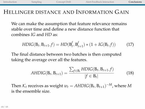
HELLINGER DISTANCE AND INFORMATION GAIN
We can make the assumption that feature relevance remainsstable over time and define a new distance function thatcombines IG and HD as:
HDIG(Bt,Bt+1, f ) = HD(Bft ,B
ft+1) ∗ (1 + IG(Bt, f )) (17)
The final distance between two batches is then computedtaking the average over all the features.
AHDIG(Bt,Bt+1) =
∑f∈Bt
HDIG(Bt,Bt+1, f )
|f ∈ Bt|(18)
Then Kt receives as weight wt = AHDIG(Bt,Bt+1)−M, where Mis the ensemble size.
68/ 68

Introduction Sampling Concept Drift Alert-Feedback Interaction Conclusions
ADAPTIVE WEIGHTING II
Let FAWt
be the feedbacks requested by AWt and FFt be the
feedbacks requested by Ft. Let Y+t (resp. Y−t ) be the fraudulent
(resp. genuine) transactions at day t (Bt), we define thefollowing sets:
I CORRFt = FAWt∩ FFt ∩ Y+
t .
I ERRFt = FAWt∩ FFt ∩ Y−t .
I MISSFt = FAWt∩ {Bt \ FFt} ∩ Y+
t .
68/ 68

Introduction Sampling Concept Drift Alert-Feedback Interaction Conclusions
ADAPTIVE WEIGHTING IIIn the example below we have |CORRFt | = 4, |ERRFt | = 2 and|MISSFt | = 3.
FAWt
FFt
FWDt
Bt
Figure : Feedbacks requested by AWt (FAW
t) are a subset of all the
transactions of day t (Bt). FFt ( FWDt
) denotes the feedbacks requestedby Ft (WD
t ). The symbol + is used for frauds and − for genuinetransactions.
68/ 68

Introduction Sampling Concept Drift Alert-Feedback Interaction Conclusions
ADAPTIVE WEIGHTING IIIWe can now compute some accuracy measures of Ft in thefeedbacks requested by AW
t :I accFt = 1− |ERRFt |
kI accMissFt = 1− |ERRFt |+|MISSFt |
kI precisionFt =
|CORRFt |k
I recallFt =|CORRFt ||FAW
t∩Y+
t |
I aucFt = probability that fraudulent feedbacks rank higherthan genuine feedbacks in FAW
taccording to PFt .
I probDifFt = difference between the mean of PFt calculatedon the frauds and the mean on the genuine in FAW
t.
If we choose aucFt as metric for Ft and similarly aucWDt
forWDt ,
then αt+1 is:αt+1 =
aucFt
aucFt + aucWDt
(19)
68/ 68
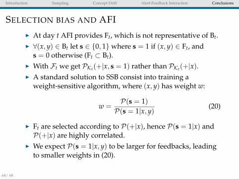
Introduction Sampling Concept Drift Alert-Feedback Interaction Conclusions
SELECTION BIAS AND AFII At day t AFI provides Ft, which is not representative of Bt.I ∀(x, y) ∈ Bt let s ∈ {0, 1}where s = 1 if (x, y) ∈ Ft, and
s = 0 otherwise (Ft ⊂ Bt).I With Ft we get PKt(+|x, s = 1) rather than PKt(+|x).I A standard solution to SSB consist into training a
weight-sensitive algorithm, where (x, y) has weight w:
w =P(s = 1)
P(s = 1|x, y)(20)
I Ft are selected according to P(+|x), hence P(s = 1|x) andP(+|x) are highly correlated.
I We expect P(s = 1|x, y) to be larger for feedbacks, leadingto smaller weights in (20).
68/ 68

Introduction Sampling Concept Drift Alert-Feedback Interaction Conclusions
INCREASING δ AND SSB CORRECTION
Table : Average Pk when δ = 15.
(a) slidingdataset classifier mean sd
2013 F 0.67 0.242013 WD 0.54 0.222013 AW 0.72 0.202014 F 0.67 0.272014 WD 0.56 0.272014 AW 0.71 0.252015 F 0.71 0.212015 WD 0.62 0.212015 AW 0.76 0.19
(b) ensembledataset classifier mean sd
2013 F 0.67 0.232013 ED 0.48 0.232013 AE 0.72 0.212014 F 0.67 0.282014 ED 0.49 0.272014 AE 0.70 0.252015 F 0.71 0.222015 ED 0.56 0.182015 AE 0.75 0.20
Table : Average Pk of Ft with methods for SSB correction (δ = 15).
dataset SSB correction mean sd2013 SJA 0.66 0.242013 weigthing 0.64 0.252014 SJA 0.66 0.272014 weigthing 0.65 0.282015 SJA 0.71 0.222015 weigthing 0.68 0.23
68/ 68

Introduction Sampling Concept Drift Alert-Feedback Interaction Conclusions
TRAINING SET SIZE AND TIME
●●●
●●●●●●●●●●●●● ●●●●●●●●●●●●●●●0e+00
1e+06
2e+06
3e+06
delayed feedback
Classifier
Tra
inin
g se
t siz
e
adaptationslidingensemble
(a) Training set size
●●●●
● ●●0
100
200
300
400
delayed feedback
Classifier
Tra
inin
g tim
e
adaptationslidingensemble
(b) Training time
Figure : Training set size and time (in seconds) to train a RF for thefeedback (Ft) and delayed classifiers (WD
t and EDt ) in the 2013 dataset.
68/ 68

Introduction Sampling Concept Drift Alert-Feedback Interaction Conclusions
FEATURE IMPORTANCE
●
●
●
●
●
●
●
●
●
●
●
●
●
●
●
●
●
●
●
●
●
●
●
●
●
●
●
●
●
●
●
●
TX_ACCEPTEDHAD_REFUSED
NB_REFUSED_HISTX_INTL
HAD_TRX_SAME_SHOPTX_3D_SECURE
IS_NIGHTHAD_LOT_NB_TX
RISK_GENDERNB_TRX_SAME_SHOP_HIS
RISK_CARD_BRANDRISK_D_AGE
RISK_LANGUAGEHAD_TEST
RISK_D_AMTRISK_TERM_MCC_GROUP
TX_HOURRISK_BROKER
RISK_TERM_MCCGRISK_LAST_COUNTRY_HIS
AGERISK_D_SUM_AMT
RISK_TERM_REGIONRISK_TERM_MCC
NB_TRX_HISRISK_TERM_COUNTRY
AMOUNTRISK_TERM_CONTINENT
MIN_AMT_HISSUM_AMT_HIS
RISK_LAST_MIDUID_HISRISK_TERM_MIDUID
0 20 40 60
Feature importance
RF model day 20130906
Figure : Average feature importance measured by the mean decreasein accuracy calculated with the Gini index in the RF models ofWD
t inthe 2013 dataset. The randomForest package [15] available in R usethe Gini index as splitting criteria.
68/ 68


