
Aalborg Universitet
Droop-free Distributed Control for AC Microgrids
Nasirian, Vahidreza ; Shafiee, Qobad; Guerrero, Josep M.; L. Lewis, Frank ; Davoudi, Ali
Published in:I E E E Transactions on Power Electronics
DOI (link to publication from Publisher):10.1109/TPEL.2015.2414457
Publication date:2016
Document VersionEarly version, also known as pre-print
Link to publication from Aalborg University
Citation for published version (APA):Nasirian, V., Shafiee, Q., Guerrero, J. M., L. Lewis, F., & Davoudi, A. (2016). Droop-free Distributed Control forAC Microgrids. I E E E Transactions on Power Electronics, 31(2), 1600 - 1617 . DOI:10.1109/TPEL.2015.2414457
General rightsCopyright and moral rights for the publications made accessible in the public portal are retained by the authors and/or other copyright ownersand it is a condition of accessing publications that users recognise and abide by the legal requirements associated with these rights.
? Users may download and print one copy of any publication from the public portal for the purpose of private study or research. ? You may not further distribute the material or use it for any profit-making activity or commercial gain ? You may freely distribute the URL identifying the publication in the public portal ?
Take down policyIf you believe that this document breaches copyright please contact us at [email protected] providing details, and we will remove access tothe work immediately and investigate your claim.
Downloaded from vbn.aau.dk on: maj 31, 2018
1
This document downloaded from www.microgrids.et.aau.dk is the preprint version of the final paper: V. Nasirian, Q. Shafiee, J. M. Guerrero, F. Lewis, and A. Davoudi, “Droop-free Distributed Control for AC Microgrids,” IEEE Transactions on Power Electronics, Early Access 2015.
Abstract
A cooperative distributed secondary/primary control paradigm for AC microgrids is proposed. This solution replaces the
centralized secondary control and the primary-level droop mechanism of each inverter with three separate regulators: voltage,
reactive power, and active power regulators. A sparse communication network is spanned across the microgrid to facilitate limited
data exchange among inverter controllers. Each controller processes its local and neighbors’ information to update its voltage
magnitude and frequency (or, equivalently, phase angle) set points. A voltage estimator finds the average voltage across the
microgrid, which is then compared to the rated voltage to produce the first voltage correction term. The reactive power regulator at
each inverter compares its normalized reactive power with those of its neighbors, and the difference is fed to a subsequent PI
controller that generates the second voltage correction term. The controller adds the voltage correction terms to the microgrid rated
voltage (provided by the tertiary control) to generate the local voltage magnitude set point. The voltage regulators collectively adjust
the average voltage of the microgrid at the rated voltage. The voltage regulators allow different set points for different bus voltages
and, thus, account for the line impedance effects. Moreover, the reactive power regulators adjust the voltage to achieve proportional
reactive load sharing. The third module, the active power regulator, compares the local normalized active power of each inverter
with its neighbors’ and uses the difference to update the frequency and, accordingly, the phase angle of that inverter. The global
dynamic model of the microgrid, including distribution grid, regulator modules, and the communication network, is derived, and
controller design guidelines are provided. Steady-state performance analysis shows that the proposed controller can accurately
handle the global voltage regulation and proportional load sharing. An AC microgrid prototype is set up, where the controller
performance, plug-and-play capability, and resiliency to the failure in the communication links are successfully verified.
Index Terms— AC microgrids, Cooperative control, Distributed control, Droop control, Inverters
This work was supported in part by the National Science Foundation under grants ECCS-1137354 and ECCS-1405173 and in part by the U.S. Office of Naval Research under grant N00014-14-1-0718. Vahidreza Nasirian, Frank L. Lewis, and Ali Davoudi are with the Department of Electrical Engineering, University of Texas, Arlington, TX 76019 USA and are also with the University of Texas at Arlington Research Institute (UTARI), Fort Worth, TX 76118 USA (emails: [email protected]; [email protected]; [email protected]). Qobad Shafiee and Josep M. Guerrero are with the Department of Energy Technology, Aalborg University, Denmark. Qobad Shafiee was also on leave with the University of Texas, Arlington, TX ([email protected]; [email protected]).
Droop-free Distributed Control for AC Microgrids
Vahidreza Nasirian, Student Member, IEEE, Qobad Shafiee, Student Member, IEEE, Josep M. Guerrero, Senior Member, IEEE, Frank L. Lewis, Fellow, IEEE, and Ali Davoudi, Member, IEEE

2
I. INTRODUCTION
Microgrids are small-scale power systems that can island from the legacy grid. They have gained popularity in distribution
systems for their improved efficiency, reliability, and expandability [1]–[6]. DC energy resources, e.g., photovoltaic arrays,
storage elements, and fuel cells, are commonly connected to the AC microgrid distribution network via voltage-source
inverters [7], [8]. A three-tier hierarchical control structure is conventionally adopted for the microgrid operation [9], [10]. The
primary control, usually realized through a droop mechanism, operates on a fast timescale and regulates inverters’ output
voltage and handles proportional load sharing among inverters [9]. It shares the total load demand among sources in proportion
to their power ratings and is commonly practiced to avoid overstressing and aging of the sources [7]–[9]. The secondary
control, in an intermediate timescale, compensates for the voltage and frequency deviations caused by the primary control by
updating inverter voltage set points [11]–[13]. Ultimately, the tertiary control carries out the scheduled power exchange with
the main grid over a longer timescale [14], [15].
Droop mechanism, or its variations [16]–[27], is a common decentralized approach to realize the primary control, although
alternative methods (e.g., virtual oscillator control [28]–[31]) are emerging. They emulate virtual inertia for AC systems and
mimic the role of governors in traditional synchronous generators [32]. Despite simplicity, the droop mechanisms suffers from
1) load-dependent frequency/voltage deviation, 2) poor performance in handling nonlinear loads [33], and 3) poor reactive
power sharing in presence of unequal bus voltages [34]. Unequal bus voltages are indispensible in practical systems to perform
the scheduled reactive power flow. Droop techniques cause voltage and frequency deviations and, thus, a supervisory
secondary control is inevitable to update the set points of the local primary controls [35]–[40]. For example, GPS-coordinated
time referencing handles frequency synchronization across the microgrid in [33], [38], [39]. Such architecture requires two-
way high bandwidth communication links between the central controller and each inverter. This protocol adversely affects the
system reliability as failure of any communication link hinders the functionality of the central controller and, thus, the entire
microgrid. The central controller itself is also a reliability risk since it imposes a single point-of-failure. Scalability is another
issue for that it adds to the complexity of the communication network and it requires updating the settings of the central
controller.
Spatially dispersed inverter-based microgrids naturally lend themselves to distributed control techniques to address their
synchronization and coordination requirements. Distributed control architectures can discharge duties of a central controller
while being resilient to faults or unknown system parameters. Distributed synchronization processes necessitate that each agent
(i.e., the inverter) exchange information with other agents according to some restricted communication protocol [5], [41], [42].
These controllers can use a sparse communication network and have less computational complexity at each inverter controller
[43]. Networked control of parallel inverters in [44], [45] embeds the functionality of the secondary control in all inverters, i.e.,

3
it requires a fully connected communication network. The master node in the networked master-slave methods [46]–[48] is still
a single point-of-failure. Distributed cooperative control is recently introduced for AC [49]–[51] and DC microgrids [52]–[55].
Distributed control of AC microgrids are also discussed in [56]–[58] (using a ratio-consensus algorithm), [50] (a multi-
objective approach), and [59]-[62] (using a distributed averaging proportional controller). Majority of such approaches are still
based on the droop mechanism (and, thus, inherit its shortcoming), require system information (e.g., number of inverters,
inverter parameters, and total load demand), require frequency measurement, and mainly handle active power sharing and
frequency regulation (or, only reactive power sharing/voltage control). Recent works of the authors in [50] and [51] investigate
distribution networks with negligible line impedances and, potentially, can lack satisfactory performance in practical multi-
terminal distribution systems with intricate and lossy transmission networks. They also assign a single source as leader, who
relays the rated frequency and voltage set points to other sources through a communication network. Moreover, such solutions
focus on the islanded mode of operation and their extension to grid-connected mode is not straightforward.
This paper provides a comprehensive distributed cooperative solution that satisfies both the secondary and the primary
control objectives for an autonomous AC microgrid without relying on the droop mechanism. Herein, each inverter is
considered as an agent of a multi-agent system (i.e., the microgrid); each inverter exchanges data with a few other neighbor
inverters and processes the information to update its local voltage set points and synchronize their normalized power and
frequencies. The proposed controller includes three modules: voltage regulator, reactive power regulator, and active power
regulator. The salient features of the proposed control method are:
• Cooperation among inverters on a communication graph provides two voltage correction terms to be added to the rated
voltage and adjust the local voltage set points of individual inverters.
• Cooperation among voltage, reactive power, and active power regulators effectively carries out global voltage regulation,
frequency synchronization, and proportional load sharing, particularly, in practical networks where the transmission/
distribution line impedances are not negligible.
• Normally, the controllers share the total load among sources in proportion to their rated active and reactive powers;
however, the rated values, embedded in the controller, can be manipulated to achieve any desired load sharing.
• The voltage regulator seeks to adjust the average voltage across the microgrid, rather than the individual inverter busses, at
the rated voltage value, and ensures global voltage regulation without the need to run a power flow analysis.
• The control method does not employ any droop mechanism and does not require any frequency measurement.
• The proposed scheme does not require prior knowledge of system parameters or the number of inverters. Thus, it features
scalability, modularity, robustness (independent of loads), and plug-and-play capability.
4
• Only a sparse communication graph is sufficient for the limited message passing among inverters. This is in direct contrast
with the centralized control approaches that require high-bandwidth bidirectional communication networks, or existing
networked control techniques that require fully-connected communication graphs.
The rest of this paper is outlined as follows: Section II discusses the proposed control methodology. Section III provides
dynamic/static model of the entire microgrid including the physical distribution grid, control modules, and communication
network, and shows that the controller objectives are also met in the steady state. The controller performance is experimentally
verified using an AC microgrid prototype in Section IV. Section V concludes the paper.
II. PROPOSED COOPERATIVE CONTROL FRAMEWORK
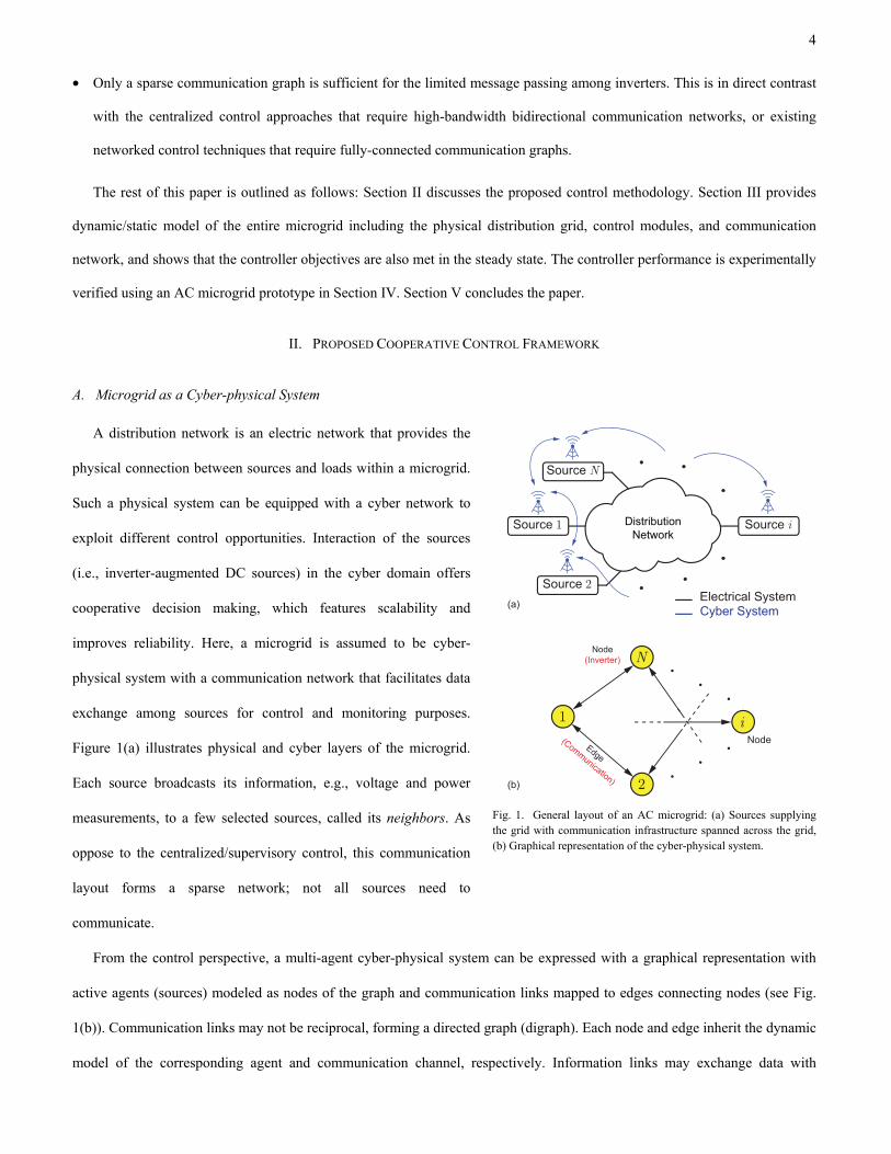
A. Microgrid as a Cyber-physical System
A distribution network is an electric network that provides the
physical connection between sources and loads within a microgrid.
Such a physical system can be equipped with a cyber network to
exploit different control opportunities. Interaction of the sources
(i.e., inverter-augmented DC sources) in the cyber domain offers
cooperative decision making, which features scalability and
improves reliability. Here, a microgrid is assumed to be cyber-
physical system with a communication network that facilitates data
exchange among sources for control and monitoring purposes.
Figure 1(a) illustrates physical and cyber layers of the microgrid.
Each source broadcasts its information, e.g., voltage and power
measurements, to a few selected sources, called its neighbors. As
oppose to the centralized/supervisory control, this communication
layout forms a sparse network; not all sources need to
communicate.
From the control perspective, a multi-agent cyber-physical system can be expressed with a graphical representation with
active agents (sources) modeled as nodes of the graph and communication links mapped to edges connecting nodes (see Fig.
1(b)). Communication links may not be reciprocal, forming a directed graph (digraph). Each node and edge inherit the dynamic
model of the corresponding agent and communication channel, respectively. Information links may exchange data with
Fig. 1. General layout of an AC microgrid: (a) Sources supplying the grid with communication infrastructure spanned across the grid, (b) Graphical representation of the cyber-physical system.
1
2
N
i
(b)
Node
Node(Inverter)
Edge
(Communication)
Source N
Distribution Network
(a)
Source 1
Source 2
Source i
Electrical SystemCyber System

5
different gains referred to as the communication weights. For example, if Node j broadcasts data jx to Node i through a link
with designated a weight of 0ija > , then, the information received at node i is
ij ja x . Generally, 0
ija > if Node i receives
data from Node j and 0ija = , otherwise. Such a graph is usually represented by an associated adjacency matrix
GA N N
ija ´é ù= Îê úë û that carries the communication weights, where N is the number of dispatchable sources. Communication
weights can be time varying and may include some channel delay; however, this study assumes time-invariant and scalar
adjacency matrix. iN denotes the set of all neighbors of Node i. The in-degree and out-degree matrices { }in indiag
id=D and
{ }out outdiagid=D are diagonal matrices with in
i
i ijj N
d aÎ
= å and out
j
i jii N
d aÎ
= å , respectively. The Laplacian matrix is defined
as in -G
L D A , whose eigenvalues determine the global dynamics of the entire system (i.e., the microgrid) [63], [64]. The
Laplacian matrix is balanced if the in-degree and out-degree matrices are equal; particularly, an undirected (bidirectional) data
network satisfies this requirement. A direct path from Node i to Node j is a sequence of edges that connects the two nodes. A
digraph is said to have a spanning tree if it contains a root node, from which, there exists at least a direct path to every other
node. Here, a graph is called to carry the minimum redundancy if it contains enough redundant links that, in the case of any
single link failure, it remains connected and presents a balanced Laplacian matrix.
B. Proposed Cooperation Policy
The proposed method requires a communication graph with the adjacency matrix N Nija ´é ù= Îê úë ûG
A that 1) has at least a
spanning tree, 2) can be undirected or directional, yet with a balanced Laplacian matrix, and 3) the graph must carry the
minimum redundancy. Communication weights, ija , are design parameters. Each source exchanges a vector of information,
norm norm, ,i i i i
e p qé ùY = ê úë û, with its neighbor sources on the communication graph, where i
e is the estimation of the averaged
voltage magnitude across the microgrid, processed at Node i . norm rated
i i ip p p and norm rated
i i iq q q are the normalized
active and reactive powers supplied by Source i . ip and i
q are the measured active and reactive powers supplied by Source
i , respectively, and rated
ip and rated
iq are the rated active and reactive powers of the same source. The control strategy attempts
to share the load among sources in proportion to their rated powers.
Objectives of the secondary/primary controller are 1) global voltage regulation, 2) frequency synchronization, 3) active
power sharing, and 4) reactive power sharing. Generally, fine adjustment of the voltage magnitude and frequency can satisfy
all four objectives. Particularly, active and reactive power flow can be managed by tuning the frequency and voltage
magnitude, respectively. The proposed control method is established on this notion. Figure 2 shows the schematic of the
control policy for Node i (Source i). The controller consists of three separate modules: the voltage regulator, reactive power
regulator, and active power regulator.
6
The controller at Node i receives information vectors of its neighbors, j
Y s, and processes the neighbors’ and local data, iY , to
update its voltage set point. *
ie and *
iw are the set points of the (line to neutral) voltage magnitude (rms value) and frequency,
respectively. Accordingly, the Space Vector PWM (SVPWM) module generates the actual voltage set point, *
iv ,
* * *
0
( ) ( ) 2 sin ( )d ,t
i i iv t e t w t t
æ ö÷ç ÷ç= ÷ç ÷ç ÷çè øò
(1)
and assigns appropriate switching signals to drive the inverter module [65]. It should be noted that the controller is assumed
activated at 0t = . As seen in Fig. 2, each inverter is followed by an LCL filter to attenuate undesired (switching and line-
frequency) harmonics. The set point in (1) is the reference voltage for the output terminal of the filtering module or,
equivalently, the microgrid bus that corresponds to Source i .
The voltage and reactive power regulator modules adjust the set point of the voltage magnitude by producing two voltage
correction terms, 1
ied and 2
ied , respectively, as
1 2
rated( ) ( ) ( ),i i ie t e e t e td d* = + + (2)
where ratede is the rated voltage magnitude of the microgrid. Regardless of the operating mode, i.e., islanded or grid-connected
modes, the rated voltage can be safely assumed equal for all active nodes (dispatchable sources). The voltage regulator at Node
i includes an estimator that finds the global averaged voltage magnitude, i.e., the averaged voltage across the microgrid. This
Fig. 2. Proposed cooperative secondary control for the Source i, of the AC microgrid. Note data exchange with the neighbor nodes.
Control Layer
Inverter i(3 Phase)
Energy Source
SVPW
M
LCL Filter
Mic
rogr
id D
istri
butio
n B
us
VoltageEstimator
Voltage regulator
Reactive power regulator
Tert
iary
Con
trol
Uni
tProposed Cooperative Secondary/ Primary Control at Node i
( )iH s
( )iG s
Nei
ghbo
rs’ D
ata
ie 1
ieδj
e
ratede
2ieδ
Active power regulator
iδω
ratedω
*ie
*iω
Power, Voltage Measurement
Physical Layer
Cyber Layer (Communication Network)
Node 1
Node N
Node 2
Node i
( )norm norm
i
ij j ij N
ba q q∈
−∑normjq
normjp ( )norm norm
i
ij j ij N
ca p p∈
−∑
Data Format:
ij N∈
norm norm, ,j j j je q p⎡ ⎤Ψ = ⎢ ⎥⎣ ⎦
Data Format:norm norm, ,
i i i ie q p⎡ ⎤Ψ = ⎢ ⎥⎣ ⎦
rated rated,e ω⎡ ⎤Ψ = ⎢ ⎥⎣ ⎦
Data Format:
rate
dra
ted
,e
ω⎡
⎤Ψ=⎢
⎥⎣
⎦
Dat
a Fo
rmat
:
7
estimation is, then, compared with the rated voltage, ratede , and the difference is fed to a PI controller, i
G , to generate the first
voltage correction term, 1
ied , and, thus, handle global voltage regulation. Accordingly, the voltage regulators collectively
adjust the average voltage of the microgrid on the rated value, yet individual bus voltages may slightly deviate from the rated
value (typically, less than 5%). This deviation is essential in practice to navigate reactive power across the microgrid.
Therefore, the reactive power regulator at Node i adjusts an additional (i.e., the second) voltage correction term, 2
ied , to
control the supplied reactive power. This module calculates the neighborhood reactive loading mismatch, imq ,
norm norm( ),i
i ij j ij N
mq ba q qÎ
= -å
(3)
which measures how far is the normalized reactive power of the Source i from the average of its neighbors’. The coupling
gain b is a design parameter. The mismatch in (3) is then fed to a PI controller, iH , (see Fig. 2) to adjust the second voltage
correction term, 2
ied , and, accordingly, mitigate the mismatch. Performance analysis in Section III-E will show that all the
mismatch terms, in the steady state, converge to zero and, thus, all normalized reactive powers would synchronize. This
satisfies the proportional reactive power sharing among sources.
The active power regulator at Source i controls its frequency and active power. This module calculates the neighborhood
active loading mismatch to assign the frequency correction term, idw ,
norm norm( ),i
i ij j ij N
ca p pdwÎ
= -å
(4)
where the coupling gain c is a design parameter. As seen in Fig. 2, this correction term is added to the rated frequency, rated
w ,
*
rated( ) ( ),i it tw w dw= + (5)
and, thus, (1) can be written as
* *
rated
0
( ) ( ) 2 sin d .t
i i iv t e t tw dw t
æ ö÷ç ÷ç= + ÷ç ÷ç ÷çè øò
(6)
Equation (6) helps to define the phase angle set point for Source i ,
* norm norm
0
( ) ( )d .i
t
i ij j ij N
t c a p pd tÎ
-åò
(7)
According to (6)–(7), the active power regulator module keeps the frequency at the rated value and fine tunes the phase angle
set point, *
id , to reroute the active power across the microgrid and mitigate the neighborhood active loading mismatch. It is
shown in Section III-E that all phase angles, *
id , will converge to their steady-state values and, thus, all frequency correction
terms, idw , decay to zero. Therefore, the microgrid frequency synchronizes to the rated frequency,
ratedw , without any
frequency measurement loop, while the controller stabilizes the phase angles, id . Indeed, transient variations in the inverter

8
frequency adjust its phase angle and control the active power flow; the frequency will not deviate from the rated value in the
steady state and normalized active powers will synchronize, which provides the proportional active load sharing.
The proposed controller is a general solution that can handle load sharing for variety of distribution systems; i.e.,
predominantly inductive, inductive-resistive, or primarily resistive networks. Indeed, the nature of the line impedances defines
the role of the active and reactive power regulators (see Fig. 2) for load sharing. In particular, a predominantly inductive
network naturally decouples the load sharing process; the reactive power regulator must handle the reactive load sharing by
adjusting voltage magnitude while the active power regulator would handle the active load sharing through adjusting the
frequency (or, equivalently, the phase angle). However, for other types of distribution network, active and reactive power
flows are entangled to both voltage and phase angle adjustment. For such cases, the load sharing is a collaborative task where
the two regulators (i.e., both the active and reactive power regulators) would work together to generate the desired set points.
The proposed controller, so far, assumes fixed and known power
rating for dispatchable sources. In a scenario that some sources are
non-dispatchable, i.e., renewable energy sources with stochastic power
output, the proposed controller can be augmented with the
methodology shown in Fig. 3. Supplied power by each stochastic
source is measured and reported to an auxiliary control unit. This
module runs optimization scenarios, e.g., Maximum Power Point
Tracking (MPPT), to decide the desired operating points. It also
compares the desired generation with the actual supplied power and updates the rated powers, rated
ip and rated
iq , to address any
mismatch. The proposed control routine in Fig. 2 uses the tuned rated powers to adjust the voltage and frequency set points.
With the modification in Fig. 3, the stochastic sources will be pushed to exploit their potentials (e.g., to produce maximum
power) while the controller in Fig. 2 proportionally shares the remaining load demand among dispatchable sources.
In the islanded mode, the system operational autonomy requires preset (fixed) values for the rated voltage magnitude and
frequency, ratede and rated
w , in all controllers. The voltage and frequency settings typically follow the standard ratings of the
nearby electricity grid. To further extend operational range of the proposed controller to the grid-connected mode, one can
consider adjustable voltage magnitude and frequency ratings. To this end, a tertiary controller (highlighted in Fig. 2) fine-tunes
such ratings. There is a single tertiary controller for the entire microgrid, and it uses the same communication network as the
secondary controllers, to propagate updated voltage and frequency ratings to all secondary controllers across the microgrid.
Fig. 3. Extension of the proposed controller to non-dispatchable (e.g., stochastic) energy sources.
Stochastic Source Solar, Wind, Storage, etc.
Auxiliary Control Unite.g., MPPT Controller
Power, VoltageMeasurement
Distribution Network
Proposed Controller (Fig. 2)
rated rated,i ip q
9
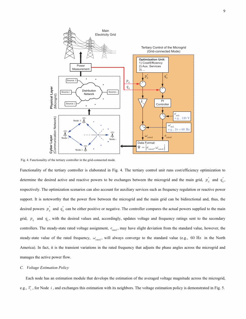
Functionality of the tertiary controller is elaborated in Fig. 4. The tertiary control unit runs cost/efficiency optimization to
determine the desired active and reactive powers to be exchanges between the microgrid and the main grid, *
dp and *
dq ,
respectively. The optimization scenarios can also account for auxiliary services such as frequency regulation or reactive power
support. It is noteworthy that the power flow between the microgrid and the main grid can be bidirectional and, thus, the
desired powers *
dp and *
dq can be either positive or negative. The controller compares the actual powers supplied to the main
grid, dp and d
q , with the desired values and, accordingly, updates voltage and frequency ratings sent to the secondary
controllers. The steady-state rated voltage assignment, ratede , may have slight deviation from the standard value, however, the
steady-state value of the rated frequency, ratedw , will always converge to the standard value (e.g., 60 Hz in the North
America). In fact, it is the transient variations in the rated frequency that adjusts the phase angles across the microgrid and
manages the active power flow.
C. Voltage Estimation Policy
Each node has an estimation module that develops the estimation of the averaged voltage magnitude across the microgrid,
e.g., ie , for Node i , and exchanges this estimation with its neighbors. The voltage estimation policy is demonstrated in Fig. 5.
Fig. 4. Functionality of the tertiary controller in the grid-connected mode.
Cyb
er L
ayer
(Com
mun
icat
ion
Net
wor
k)
Node 1
Node N
Node 2
Node i
Optimization Unit: 1) Cost/Efficiency2) Aux. Services3) ...
Tertiary Control of the Microgrid(Grid-connected Mode)
PowerMeasurement
kω
ratedω
ratede
dp
dq
dp∗
dq∗
PI Controller
std.ee.g., 120 V
e.g., 2 60 Hzπ×std.ω
rated rated,e ω⎡ ⎤Ψ = ⎢ ⎥⎣ ⎦
Data Format:
Source N
Distribution Network
Source 1
Source 2
Source i
Main Electricity Grid
Phys
ical
Lay
er(M
icro
grid
)

10
Accordingly, the estimator at Node i updates its own output, ie , by processing the neighbors’ estimates,
je s ( Î
ij N ), and
the local voltage measurement, ie ,
( )0
( ) ( ) ( ) ( ) d .i
t
i i ij j ij N
e t e t a e et t tÎ
= + -åò
(8)
This updating policy is commonly referred to as the dynamic
consensus protocol in the literature [66]. As seen in (8), the
local measurement, e.g., ie , is directly fed into the estimation
protocol. Thus, in case of any voltage variation at Node i ,
the local estimate, ie , immediately responds. The change in
ie propagates through the communication network and
affects all other estimations. Assume that T
1 2,[ , ,..., ]
Ne e e=e
and T
1 2,[ , ,..., ]
Ne e e=e are the measured voltage and the
estimated average voltage vectors, respectively. E and E
are the Laplace transforms of e and e , respectively.
Accordingly, global dynamic response of the estimation
policy is formulated in [53] as
1
est( ) ,N
s s -= + =E I L E H E (9)
where ´ÎI N NN , L , and
estH are the identity, Laplacian, and the estimator transfer-function matrices, respectively. It is
shown in [53] that if the communication graph has a spanning tree with a balanced Laplacian matrix, L , then, all elements of
e converge to a consensus value, which is the true average voltage, i.e., the average of all elements in e . Equivalently,
ss ss ss ,= =e Me e 1 (10)
where N N´ÎM is the averaging matrix, whose elements are all 1 N . ssx expresses the steady-state value of the vector
1Îx N . x is a scalar that represents the average of all elements in the vector x . 1N´Î1 is a column vector whose
elements are all one.
III. SYSTEM-LEVEL MODELING
System-level modeling studies the dynamic/static response of the entire microgrid with the proposed controller in effect.
The system under study encompasses interactive cyber and physical subsystems. The communication graph topology defies the
Fig. 5. Voltage averaging policy at each node; dynamic consensus protocol.
Voltage Estimator 1
Voltage Estimator N
Communicationwith neighbors
Cyber Layer (Communication Graph)
Node 1
Node N
Node 2
Node i
1ej
e
1j N∈ ( )
1
1 1j jj N
a e e∈
−∑
1e
je
Nj N∈
( )N
Nj j Nj N
a e e∈
−∑
Ne
Ne
Communicationwith neighbors

11
interaction among controllers, functionality of the controllers determines output characteristics of the sources, and, finally, the
transmission/distribution network rules the physical interaction among sources (and loads). Thus, the system-level study
involves in mathematical modeling of each of the subsystems and establishment of mathematical coupling between the
interactive subsystems.
A. Distribution Network Model
Dispatchable sources, transmission network, and loads form the physical layer of the microgrid. This layer is shown in Fig.
1(a), where sources are considered as controllable voltage source inverters. The proposed controller determines the voltage set
pints (both magnitude, *
ie , and phase, *
id ) for each source (i.e., inverter) by processing the supplied active and reactive powers.
Such controller acts on the physical layer, which is a multi-input/multi-output plant with the voltage set points as the inputs and
the supplied active and reactive powers as the outputs. Herein, we express the output variables, i.e., the supplied powers, in
terms of the input variables, i.e., the voltage set points.
Figure 1(a) helps to formulate the supplied current of each source. By formulating the supplied current by Source i ,
1( )
( ),N
i ii i ij i jj i
I Y V Y V V= ¹
= + -å
(11)
where iI and i
V are the phasor representation of the supplied current and phase voltage of the Source i , respectively. iiY and
ijY are the local load admittance at Bus i (Source i ) and the admittance of the transmission line connecting busses i and j ,
respectively. With no loss of generality, the distribution network is assumed reduced (i.e., by using Kron reduction) such that
all non-generating busses are removed from the network. Thus, the complex power delivered by the Source i is,
2 * * *
1 1( )
3 3 3 .N N
i i i i ij i j ijj j i
s V I V Y VV Y*
= = ¹
= = -å å
(12)
Assume i i iV e d= and
ij ij ijY y q= where i
e , ijy , i
d , and ijq are the magnitude of i
V , magnitude of ijY , phase of i
V , and
phase of ijY , respectively.
ij ij ijY g jb= + is the rectangular representation of the admittance
ijY . One can use (12) to derive the
active and reactive powers delivered by the Source i ( ip and i
q , respectively),
2
1 1( )
3 3 cos( ),N N
i i ij i j ij i j ijj j i
p e g e e y d d q= = ¹
= - - -å å
(13)
2
1 1( )
3 3 sin( ),N N
i i ij i j ij i j ijj j i
q e b e e y d d q= = ¹
= - - - -å å
(14)
The secondary control typically acts slower than the dynamic of the power network (microgrid), as its objectives are
voltage and power regulation in the steady state. Accordingly, one can safely neglect the fast dynamic transient responses of
the microgrid and use the phasor analysis in (13)–(14) to model the power flow. Equations (13)–(14) express nonlinear

12
relationships between the voltages and supplied powers. In time domain, any variable x can be represented as qx x x= +
where qx and x are the quiescent and small-signal perturbation parts, respectively. Thus, one can write,
q q
1 1
, ,1 1
ˆˆ ˆ
ˆˆ ˆ
N Ni i
i i i i j jj jj j
N Np p
i e ij j ij jj j
p pp p p p e
e
p k e kd
dd
d
= =
= =
¶ ¶= + = + +
¶ 
= +
å å
å å
(15)
q q
1 1
, ,1 1
ˆˆ ˆ
ˆˆ ˆ
N Ni i
i i i i j jj jj j
N Nq q
i e ij j ij jj j
q qq q q q e
e
q k e kd
dd
d
= =
= =
¶ ¶= + = + +
¶ 
= +
å å
å å (16)
where the coefficients in (15)–(16) are formulated,
, q1
3 ,N
p ie ii i ij
ji
pk e g
e =
= + å
(17)
q q q
,3 cos( ), p
e ij i ij i j ijk e y j id d q= - - - ¹
(18)
q q q q q 2
,1( ) 1
3 sin( ) 3 ,N N
pii i j ij i j ij i i ij
j i j
k e e y q e bd d d q= ¹ =
= - - = - -å å (19)
q q q q
,3 sin( ), p
ij i j ij i j ijk e e y j id d d q= - - - ¹
(20)
, q1
3 ,N
q ie ii i ij
ji
qk e b
e =
= - å
(21)
q q q
,3 sin( ), q
e ij i ij i j ijk e y j id d q=- - - ¹
(22)
q q q q q 2
,1( ) 1
3 cos( ) 3 ,N N
qii i j ij i j ij i i ij
j i j
k e e y p e gd d d q= ¹ =
= - - - = -å å (23)
q q q q
,3 cos( ), .q
ij i j ij i j ijk e e y j id d d q= - - ¹
(24)
Equations (15)–(24) explain how a disturbance in any of the voltage magnitudes, ie s, or phases, ˆ
id s, affects the power flow in
the entire microgrid. These equations can be represented in the matrix format,
ˆˆ ˆp pe d= +p k e k d (25) ˆˆ ˆq q
e d= +q k e k d (26)
where T
1 2ˆ ˆ ˆ ˆ, ,...,
Np p pé ù= ê úë ûp ,
T
1 2ˆ ˆ ˆ ˆ, ,...,
Nq q qé ù= ê úë ûq ,
T
1 2ˆ ˆ ˆ ˆ, ,...,
Ne e eé ù= ê úë ûe , and
T
1 2ˆ ˆ ˆ ˆ, , ...,
Nd d dé ù= ê úë ûd are column vectors carrying
small-signal portions of the active powers, reactive powers, voltage magnitudes, and voltage phases, respectively. ,
[ ]p pe e ij
k=k ,
,[ ]p p
ijkd d=k ,
,[ ]q q
e e ijk=k , and
,[ ]q q
ijkd d=k are all matrices in N N that contain coefficients in (17)–(24). p
dk and qek are
referred to here as the p d- and q e- transfer matrices, respectively.
B. Dynamic Model of the Control and Cyber Subsystems
The cyber domain is where the controllers exchange measurements, process information and, update the voltage set points.
Interactions and functionality of the controllers are shown in Fig. 2. One can see how the voltage and reactive power regulators
cooperate to adjust the voltage magnitude set points, *
ie . In the frequency domain,
( ) 1
rated( ) ,i i iG s E E E- = D
(27)
norm norm 2( ) ( ) ,i
i ij j i ij N
H s ba Q Q EÎ
æ ö÷ç ÷ç - =D÷ç ÷ç ÷çè øå
(28)
1 2 *
rated,
i i iE E E E+D +D = (29)
where ratedE , i
E , 1
iED , norm
iQ , 2
iED , and *
iE are the Laplace transforms of rated
e , ie , 1
ieD , norm
iq , 2
ieD , and *
ie ,
respectively. Equations (27)–(29) can be represented in the matrix format,
13
( ) ( ) 1
rated rated est,- = - =G E E G E H E ED (30) norm 1 2
rated,b b -- =- =HLQ HLq Q ED (31)
1 2 *
rated,+ + =E E E ED D (32)
where diag{ }iG=G and diag{ }
iH=H are diagonal matrices containing voltage and reactive power controllers,
respectively. G and H are referred to as the voltage-controller and Q -controller matrices, respectively.
rated
rateddiag{ }
iq=q is a diagonal matrix that carries the rated reactive powers of the sources. rated rated
E=E 1 ,
T1 1 1 1
2, , ...,i NE E Eé ù= D D Dê úë ûED ,
T2 2 2 2
2, , ...,i NE E Eé ù= D D Dê úë ûED ,
T* * * *
1 2, , ...,
NE E Eé ù= ê úë ûE , and
Tnorm norm norm norm
1 2, , ...,
NQ Q Qé ù= ê úë ûQ are column vectors carrying control variables.
It is assumed that for 0t < all sources of the microgrid operate with identical voltage set points, i.e., for all 1 i N£ £ ,
*
ra tedie e= and *
ratediw w= and, thus, rated rated
( ) sin( )iv t e tw= . Then, the proposed controller is activated at 0t = . Thus, the
quiescent value of any variable x , qx , represents its steady-state value for 0t < , i.e., before activating the controller, and the
small-signal part, x , captures the variable response to the controller activation for 0t > . Therefore, one can safely write
T1,q 1,q 1,q 1,q
1 2, , ...,
Ne e ed d dé ù= =ê úë ûe 0d ,
T2,q 2,q 2,q 2,q
1 2, , ...,
Ne e ed d dé ù= =ê úë ûe 0d , and q
rated ratede=e 1 and, accordingly, simplify (30)–(31),
( ) 1
rated estˆ ˆ ˆ ,- =G E H E ED
(33)
q1 2
ratedˆ ˆ ,b
s-
æ ö÷ç ÷ç- + =÷ç ÷÷çè ø
qHLq Q ED
(34)
where T
q q q q
1 2, , ...,
Nq q qé ù= ê úë ûq carries the reactive powers supplied by individual sources for 0t < . Since the rated voltage does
not change before and after activating the controller, ratedˆ =E 0 . The voltage set points dynamics can now be found by
substituting (33)–(34) into (32),
q
* 1
est ratedˆ ˆ ˆ .b
s-
æ ö÷ç ÷ç= - - + ÷ç ÷÷çè ø
qE GH E HLq Q
(35)
As seen, (35) has two terms. The first term, estˆ-GH E , represents the controller effort to achieve the global voltage regulation,
and, the second term, ( )1 q
ratedˆb s-- +HLQ q Q , explains how the controller balances reactive load sharing across the microgrid.
Active power regulators (see Fig. 2) adjust the active power flow by tuning the phase angles. The controller at each source,
e.g., Source i, compares its normalized active power with those of its neighbors and, accordingly, updates the phase angle set
point as in (7). Controller activation at 0t = implies that *
rated( 0)itw w< = and, thus, q ss( 0) 0
i itd d= < = . Accordingly,
* norm norm
0
ˆ ( 0) ( ) d .i
t
i ij j ij N
t ca p pd tÎ
³ = -åò
(36)
Equivalently, in the frequency domain,
* norm norm1ˆ ( ) ,
i
i ij j ij N
ca P Ps Î
æ ö÷ç ÷çD = - ÷ç ÷ç ÷çè øå
(37)
14
where *ˆi
D is the Laplace transform of *
id . One can write (37) in the matrix format,
q
* 1 1
rated ratedˆ ˆ ,
c c
s s s- -
æ ö÷ç ÷ç= - = - + ÷ç ÷÷çè ø
pLp P Lp PD
(38)
where T
* * * *
1 2ˆ ˆ ˆˆ , ,...,
Né ù= D D Dê úë ûD and rated
rateddiag{ }
ip=p is a diagonal matrix that includes the rated active powers of the
sources. T
q q q q
1 2, , ...,
Né ù= ê úë ûp p p p carries the active powers supplied by individual sources before the controller activation, i.e.,
for 0t < . Equation (38) represents the phase angles dynamic response to mitigate and, eventually, eliminate the active load
sharing mismatch.
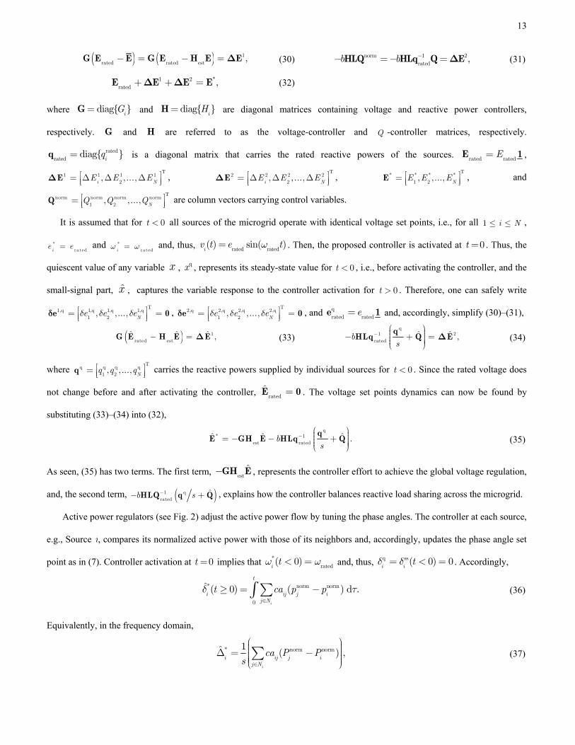
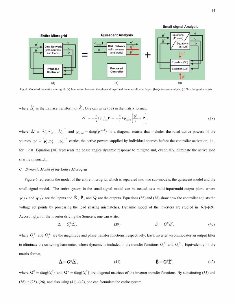
C. Dynamic Model of the Entire Microgrid
Figure 6 represents the model of the entire microgrid, which is separated into two sub-models; the quiescent model and the
small-signal model. The entire system in the small-signal model can be treated as a multi-input/multi-output plant, where
q sp and q sq are the inputs and E , P , and Q are the outputs. Equations (35) and (38) show how the controller adjusts the
voltage set points by processing the load sharing mismatches. Dynamic model of the inverters are studied in [67]–[69].
Accordingly, for the inverter driving the Source i, one can write,
*ˆ ˆ ,i i iGDD = D (39) *ˆ ˆ ,E
i i iE G E= (40)
where EiG and i
G D are the magnitude and phase transfer functions, respectively. Each inverter accommodates an output filter
to eliminate the switching harmonics, whose dynamic is included in the transfer functions EiG and i
G D . Equivalently, in the
matrix format,
*ˆ ˆ ,D=GD D (41) *ˆ ˆ ,E=E G E (42)
where diag{ }E EiG=G and diag{ }
iGD D=G are diagonal matrices of the inverter transfer functions. By substituting (35) and
(38) in (25)–(26), and also using (41)–(42), one can formulate the entire system.
Fig. 6. Model of the entire microgrid: (a) Interaction between the physical layer and the control/cyber layer, (b) Quiescent analysis, (c) Small-signal analysis.
(b)(a) (c)
Dist. Network(with sources
and loads)
Proposed Controller
*eδ*
qp
qqratede 1
0
*e
δ*ˆpq
p
Entire Microgrid
Dist. Network(with sources
and loads)
Proposed Controller
Quiescent Analysis
eq
qe
Small-signal Analysis
Equations (41)-(42)
Equations (25)-(26)
e
Equation (38)
Equation (35)
qp
qq+=
15
It is commonly assumed that the transmission/distribution network is predominantly inductive and, thus, active and reactive
powers are mainly controlled by adjusting the voltage phases and magnitudes, respectively [70]. This assumption implies that
in (25) and (26), pek 0 and q
dk 0 , respectively, which helps to find the reduced-order dynamic model of the entire system.
Substituting (41) in (38) and (42) in (35) yields
( )q1
1
ratedˆ ˆ ,
c
s s
-D -
æ ö÷ç ÷ç= - + ÷ç ÷÷çè ø
pG Lp PD
(43)
( )q1
1
est ratedˆ ˆ .E b
s
--
æ öæ ö ÷ç÷ç ÷ç+ = - +÷ ÷ç ç÷ç ÷è ø ÷çè ø
qG GH E HLq Q
(44)
Substituting the reduced form of (25)–(26) in (43)–(44) yields
q1
ratedˆ ,
P s-=-p
P T Lp
(45)
q1
ratedˆ ,
Q s-=-q
Q T Lq
(46)
where, PT and
QT are the P –balancing and Q –balancing matrices, and are defied as,
( )1
11
rated,p
Ps c d
--
D -æ ö÷ç + ÷ç ÷çè øT k G Lp
(47)
( ) ( )1
1 11 1 1
est rated.q E q
Q e eb b
-- -
- - -æ ö÷ç + + ÷ç ÷çè øT k G H H GH k Lq
(48)
Equations (43)–(48) describe dynamic response of the entire microgrid with the proposed controller in effect. Equations (45)–
(46) describe that if the power (either active or reactive) was proportionally shared prior to activating the controller, i.e.,
1 q
ratedn- =p p 1 or 1 q
ratedm- =q q 1 , the power flow would remain intact after the controller activation, i.e., ˆ=p 0 or ˆ=q 0.
D. Controller Design Guideline
Appropriate selection of the control parameters is essential for proper operation of the proposed control methodology. For
a given microgird, converter transfer function matrices, DG and EG , rated active and reactive matrices, ratedp and rated
q ,
respectively, and p d- and q e- transfer matrices, pdk and q
ek , respectively, are known. Alternative communication networks
may be chosen to exchange information; they, however, must satisfy three requirements; it should be a sparse graph with 1) at
least a spanning tree, 2) balanced Laplacian matrix, and 3) minimum communication redundancy. Communication weights of
the graph, ija , and, thus, the Laplacian matrix, L , directly determine the voltage estimator dynamic, est
H . One may tune the
weights and examine the estimators dynamic through (9) to achieve a fast enough response. More details and insightful
guidelines for optimal design of communication weights in cooperative systems can be found in [71].
Next, the designer may adjust the controller matrices diag{ }iG=G and diag{ }
iH=H and the coupling gain b by
evaluating (48) to place all poles of QT in the Open Left Hand Plane (OLHP). Intuitively, smaller gains help to stabilize the
entire system while larger gains provide a faster dynamic response. Accordingly, the designer may decide the parameters by
16
making a trade-off between relative stability and settling time. The estimator dynamic should be considerably faster than the
microgrid dynamics. Therefore, to evaluate (48), one can safely assume estH M . Moreover, inverter switching frequency
can be assumed high enough to provide a prompt response to the voltage command, i.e., EN
G I .
As can be seen in Fig. 2, two separate modules, i.e., the voltage and the reactive power regulators, adjust the voltage
magnitude, *
ie , by generating two voltage correction terms, 1
ied and 2
ied , respectively. As discussed in Section II-B, the
voltage regulator is tasked to maintain average voltage across the microgrid at the rated value. Per such assignment, the voltage
regulator must act fast to ensure voltage stability/regulation. On the other hand, the reactive power regulator is accountable for
reactive load sharing in the steady state and its transient performance has less significance. Accordingly, the voltage control
loops (including voltage estimators, controllers iG s, and voltage measurement filters) must be designed for a higher
bandwidth compared to the reactive power control loops (involving controllers iH s and reactive power measurement filters).
Typically, voltage measurement filters have a relatively high bandwidth as they only need to remove the switching harmonics.
On the contrary, besides damping the switching harmonics, the active and reactive measurement units should filter out much
lower frequency terms of the line-frequency harmonics and other contents caused by load nonlinearity or unbalance. Such
design requirement slows down the power measurements process and, thus, the overall active/reactive load sharing control
loops. Accordingly, as a design guideline, it is sufficient to choose the reactive power controllers iH s to be slightly slower
than the voltage controllers iG s; low bandwidth power measurement filters automatically set the frequency response of the
power regulators to be quite slower than the voltage regulator module.
Next step in the design procedure considers active power regulators. Equation (45) and (47) provide dynamic response of
the active load sharing mechanism. Given the fast response of the inverters, one may assume NDG I , which simplifies (47).
The designer may sweep the coupling gain c and assess the stability and dynamic response through (47) to find an appropriate
choice for c .
E. Steady-state Performance Analysis
The design guideline in Section III-D assures stable operation of the microgrid; physical variables such as voltages
(magnitude and phase), system frequency, and supplied active and reactive powers would converge to steady-state values. This
performance analysis investigates load sharing and voltage regulation quality in the steady state. To this end, assume that the
system operates in the steady state for 0t t³ . It should be noted that although the controller stabilizes voltages across the
microgrid, one cannot simply deduce that the voltage and reactive power mismatches are zero. In other words, the inputs to the
PI controllers iG and i
H in Fig. 2 may be nonzero in the steady state, yet the two voltage correction terms 1
ied and 2
ied
17
continuously vary with opposite rates such that sum of the two terms leaves a constant value and, thus, the voltage magnitude
set point converges to a steady-state value. The following discussion attempts to show that such a scenario never happens; i.e.,
the mismatch inputs to both controllers decay to zero in the steady state, resulting in successful global voltage regulation and
reactive load sharing. It also explains that the active power mismatch terms would all decay to zero, which provides the desired
active load sharing while maintaining the rated frequency.
Voltage regulation and reactive load sharing is first to study. In the steady state, the voltage estimators converge to the true
average voltage of the microgrid. Equivalently, ss ss ss= =e Me e 1 . Thus, based on the control methodology in Fig. 2,
one can write
( )( )
1 1 ss
0 P I 0 rated2 2 -1 ss
0 P I 0 rated
( ) ( ),
( ) ( )
t t e
t t b
ìï = + + - -ïïíï = + + - -ïïî
e e G G 1 Me
e e H H Lq q
d dd d
(49)
where 1
0ed and 2
0ed are column vectors that carry the integrator outputs in i
G s and iH s at 0
t t= , respectively. Accordingly,
( )
*ss 1 2
rated
1 2 ss -1 ss
rated 0 0 P rated P rated
ss -1 ss
I rated I rated 0
( )
( ) ( ),
e e b
e b t t
= + +
= + + + - -
+ - - -
e e e e
1 e e G e 1 H Lq q
G e 1 H Lq q
d d
d d
(50)
where IG and P
G are the diagonal matrices carrying the integral and proportional gains of the voltage-controller matrix G
such that P I
s+ =G G G . Similarly, IH and P
H are the diagonal matrices carrying the integral and proportional gains of
the Q -controller matrix H . Equation (50) holds for all 0t t³ , and provides a constant voltage set point vector, *sse . Thus, the
time-varying part of (50) is zero or, equivalently,
ss -1 ss
rated rated( ) ,e - =e U1 Lq q (51)
where 1 1
I Idiag{ }
ib u- -= =U G H is a diagonal matrix. Multiplying both sides of (51) from the left by
T1 ,
ss T T -1 ss
rated rated( ) .e - =e 1 U1 1 Lq q (52)
Given the balanced Laplacian matrix, T =1 L 0 [54], which simplifies (52),
ss
rated1
( ) 0.N
ii
e u=
- =åe
(53)
Since all entries of the matrix U are positive, (53) yields ss
ratede = e , which implies that the controllers successfully regulates
the averaged voltage magnitude of the microgrid, sse , at the rated value, ratede . Moreover, by substituting ss
rated0e - =e
in (51),
-1 ss
rated.=Lq q 0 (54)
18
1Z 4
Z
34Z
12Z
23Z
Fig. 7. AC microgrid prototype: (a) Inverter modules, (b) dSAPCE processor board (DS1006), (c) Programming and monitoring PC, (d) RL loads.
Fig. 8. Schematic of the microgrid prototype; radial electrical connection and ring cyber network.
If L is the Laplacian matrix associated with a graph that contains a spanning tree, the only nonzero solution to =Lx 0 is
n=x 1 , where n is any real number [53]. Thus, (54) implies ss
ratedn=q q 1 , which assures that the controller shares the total
reactive load among the sources in proportion to their ratings.
Frequency regulation and active load sharing is the next to study. The controller guarantees the convergence of the voltage
magnitude vector, e , and phase angle vector, d to steady-state values. Thus, (6)–(7) suggest that all sources would
synchronize to the rated frequency, ratedw . Moreover, based on (7), stabilizing the phase angles across the microgrid implies
that all the frequency correction terms in (4) should decay to zero. Equivalently,
1 ss
rated,c - =Lp p 0 (55)
which offers, ss
ratedm=p p 1 , where m is a positive real number. Thus, the controller successfully handles the proportional
active load sharing.
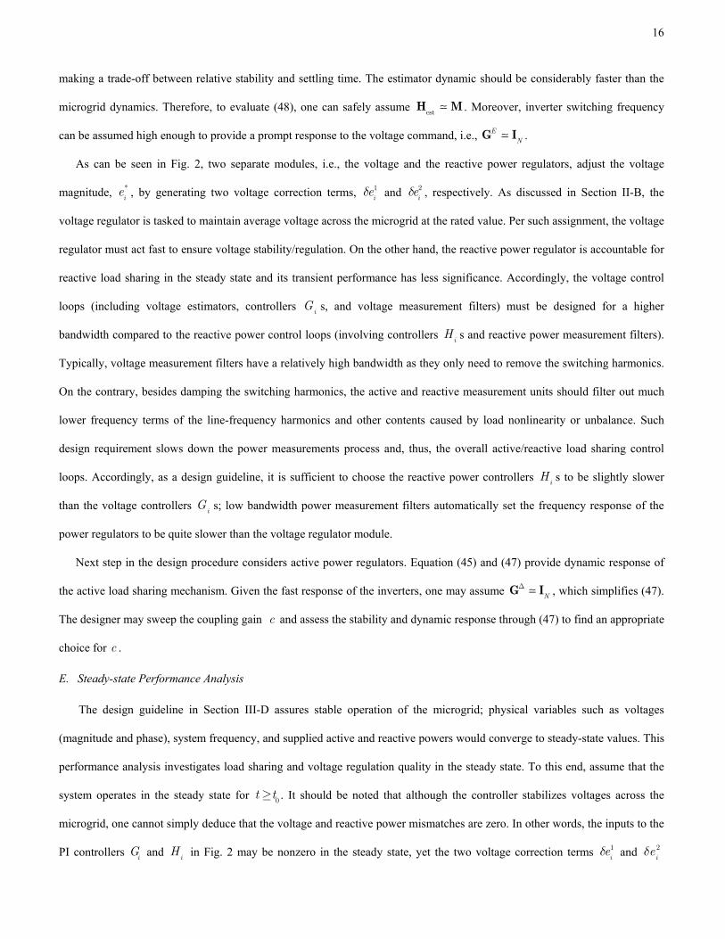
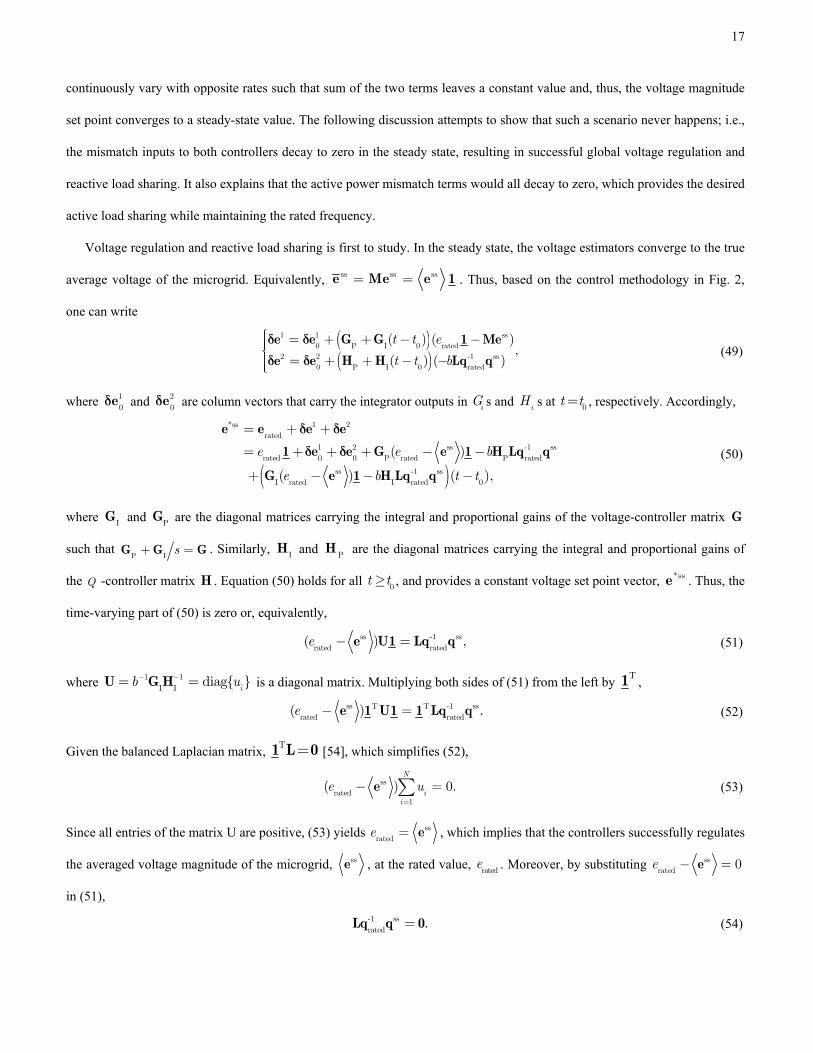
IV. EXPERIMENTAL VALIDATION
A 120 / 208 V, 60 Hz three-phase AC microgrid, shown in Fig. 7, is prototyped in the Intelligent Microgrid Laboratory at
Aalborg University. System schematic is described in Fig. 8, where four inverter-driven sources are placed in a radial
connection to supply two loads, 1Z and 4
Z . The inverters (sources) have similar topologies but different ratings, i.e., the
ratings of the inverters 1 and 2 are twice those for the inverters 3 and 4 . Each inverter is augmented with an LCL filter to
eliminate switching and line-frequency harmonics. RL -circuit model is used for each transmission line. An inductive-resistive
distribution network is adopted to investigate collaborative interaction of the active and reactive power regulators in load
sharing. Structure of the cyber network is highlighted in Fig. 8. Alternative cyber networks for a set of four agents in DC
microgrids are discussed by authors in [53], [54] where the ring structure is shown to be the most effective option and, thus, is
19
considered here. It can be seen that the ring connection provides a sparse network that carries the required minimum
redundancy, defined in Section II-A, where no single communication link failure would hinder the connectivity of the graph.
Communication links are bidirectional to feature a balanced Laplacian matrix. A dSPACE processor board (DS1006) models
the communication channels and implements the control routines. Electrical and control parameters of the microgrid are
provided in the Appendix.
A. Performance Assessment
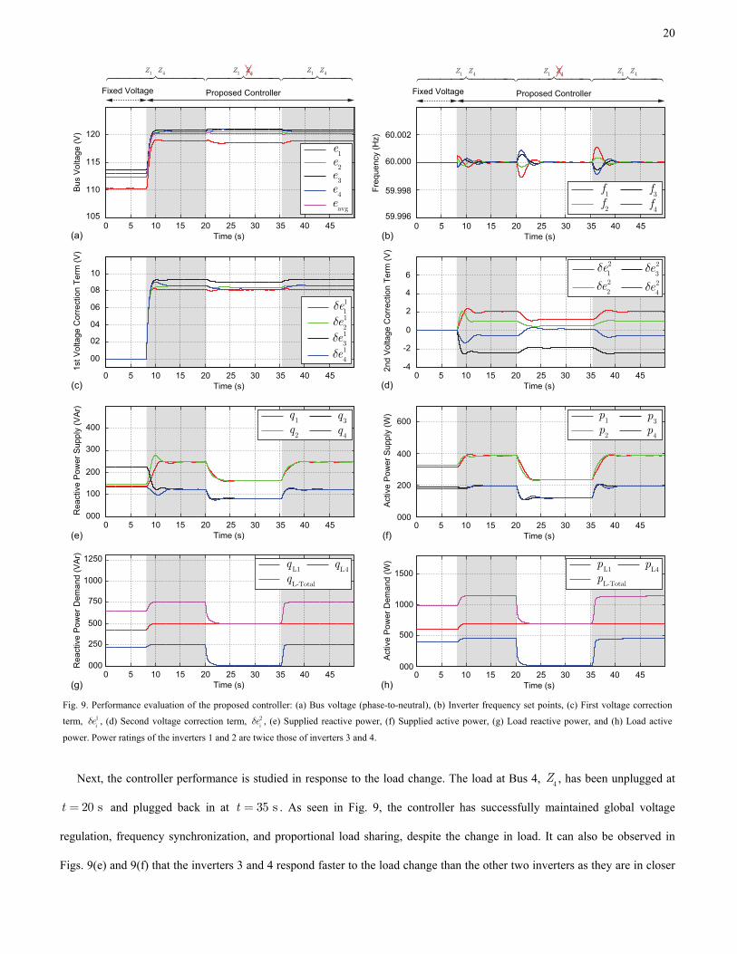
Figure 9 evaluates performance of the proposed control methodology. Inverters are initially driven with fixed voltage
command, i.e., 120 Vie* = and * 120 rad/s
iw p= . It should be noted that no voltage feedback control had been initially in
action to compensate the voltage drop across the LCL filters and, thus, the resulting bus voltages in Fig. 9(a) are less than the
desired set point, i.e., 120 Vie* = . It can also be seen in Figs. 9(e) and 8(f) that the total load is not shared among sources in
proportion to their power ratings.
It can be seen in the Appendix that the voltage controllers iG s are designed slightly faster than the reactive power
controllers iH s. Cut-off frequencies of the power measurement filters are as low as 3 Hz to damp all undesired low-
frequency harmonics. These design considerations set the dynamic responses of the two voltage and reactive power regulators
apart enough to dynamically separate the two resulting voltage correction terms, i.e., 1
ied and 2
ied . The proposed controller is
activated at 8 st = . The voltage correction terms have been added to the voltage set points to help with the global voltage
regulation and reactive load sharing. Figure 9(a) demonstrates that the controllers have boosted the bus voltages across the
microgrid to satisfy the global voltage regulation; i.e., for 8 st > , the average voltage across the microgrid is successfully
regulated at the desired 120 V . As seen in Figs. 9(b) and 9(c), the first and the second voltage correction terms respond at two
different time scales; the first correction term 1
ied (output of the voltage regulator) responds four times faster than the second
correction term 2
ied (output of the reactive power regulator). Figure 9(b) shows that the controllers have varied the frequency
set points in transients to adjust individual phase angles and provide the desired active load sharing. This figure supports the
discussions in Section III-E, where the active power regulator is proven to only enforce transient deviations in frequency and
that imposes no steady-state deviation. It can be seen that all inverter frequencies synchronize to the rated frequency of 60 Hz
in the steady state. Figures 9(e) and 9(f) show the filtered power measurements and explain how the controllers have
effectively rerouted the power flow to provide proportional load sharing. Individual and total reactive and active load demands
are plotted in Figs. 9(g) and 9(h), respectively. It should be noted that the loads have drawn more power once the controller is
activated since the voltages are boosted across the entire microgrid.
20
Fig. 9. Performance evaluation of the proposed controller: (a) Bus voltage (phase-to-neutral), (b) Inverter frequency set points, (c) First voltage correction
term, 1ied , (d) Second voltage correction term, 2
ied , (e) Supplied reactive power, (f) Supplied active power, (g) Load reactive power, and (h) Load active
power. Power ratings of the inverters 1 and 2 are twice those of inverters 3 and 4.
Next, the controller performance is studied in response to the load change. The load at Bus 4, 4Z , has been unplugged at
20 st = and plugged back in at 35 st = . As seen in Fig. 9, the controller has successfully maintained global voltage
regulation, frequency synchronization, and proportional load sharing, despite the change in load. It can also be observed in
Figs. 9(e) and 9(f) that the inverters 3 and 4 respond faster to the load change than the other two inverters as they are in closer
Fixed Voltage Proposed Controller
1 4
Z Z��������� 1 4
Z Z������� 1 4
Z Z�������
Time (s)
Freq
uenc
y (H
z)
(b)5 10 15 35 400 20 25 30 45
60.000
Time (s)
Bus
Vol
tage
(V)
(a)
1055 10 15 35 400 20 25 30 45
110
115
120
59.998
59.996
60.002
Time (s)
1st V
olta
ge C
orre
ctio
n Te
rm (V
)
(c)
00
5 10 15 35 400 20 25 30 45
02
04
06
08
10
(d) Time (s)2n
d V
olta
ge C
orre
ctio
n Te
rm (V
)
-45 10 15 35 400 20 25 30 45
0
Time (s)
Rea
ctiv
e P
ower
Sup
ply
(VA
r)
(e)
0005 10 150 20 25
100
200
300
400
35 4030 45(f) Time (s)
Act
ive
Pow
er S
uppl
y (W
)
5 10 15 35 400 20 25 30 45
-2
2
4
6
000
200
400
600
Fixed Voltage Proposed Controller
1 4
Z Z��������� 1 4
Z Z������� 1 4
Z Z�������
11eδ
12eδ
13eδ
14eδ
1q
2q
3q
4q
1p
2p
3p
4p
21eδ
22eδ
23eδ
24eδ
3f
4f
1f
2f
1e
2e
3e
4e
avge
Time (s)
Rea
ctiv
e P
ower
Dem
and
(VA
r)
(g)
0005 10 150 20 25
250
500
750
1000
35 4030 45(h) Time (s)
Act
ive
Pow
er D
eman
d (W
)
5 10 15 35 400 20 25 30 45000
500
1000
1500
1250L1q
L4q
L-Totalq
L1p
L4p
L-Totalp

21
vicinity of 4Z . Soft load change is performed in this study for safety purposes. In fact, the load inductor at Bus 4 features an
air-gap control knob. Using this control opportunity, at 20 st = , the load inductance is manually increased to its maximum
value to provide an ultimate current damping feature. Then, the load is physically unplugged. A reverse procedure is followed
at 35 st = to plug the load, 4Z , back in. This soft load change procedure, besides the damping effect of the power
measurement filters, explains why the supplied powers in Figs. 9(e) and 9(f) and the load demands in Figs. 9(g) and 9(h) show
a slow and gradual profile rather than sudden changes.
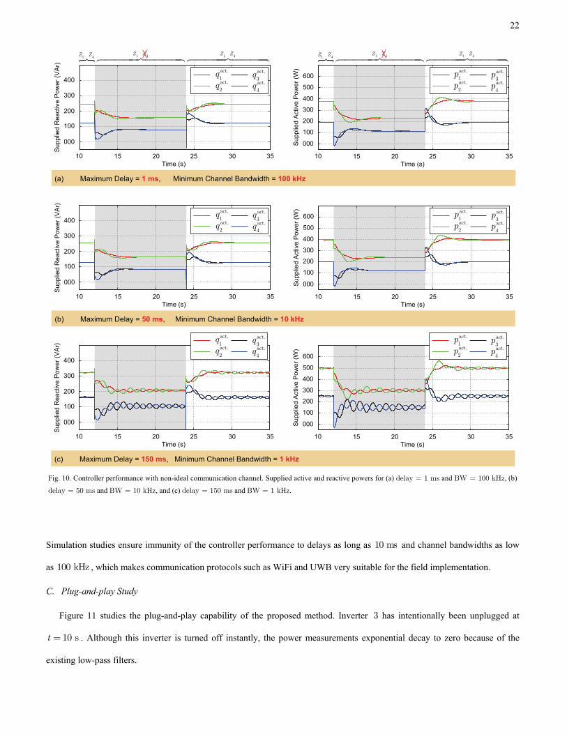
B. Communication Delay and Channel Bandwidth
Communication is indispensable to access neighbor data and, thus, to the operation of distributed systems. Accordingly,
channel non-idealities, e.g., transmission/propagation delay and limited bandwidth, and channel deficiencies such as packet
loss may compromise the overall system performance. Thus, low delay and high bandwidth communication protocols are of
paramount value for distributed control structures. For example, WiFi and Ultra Wide Band (UWB) protocols offer bandwidths
up to 5 GHz and 7.5 GHz, respectively, with delays less than 1 sm . It should be noted that the length of the communication link
directly affects the channel delay. Channel non-ideality effects on the controller performance has been studied in [72] for
distributed systems and, particularly, for microgrids in [40], [73], and [74]. It is shown that such non-idealities have a
negligible impact on the overall system performance if the channel delay is negligible compared to the controller dynamics.
For the underlying microgrid, results in Fig. 9 clearly show that the controller dynamics are in the orders of hundreds of
milliseconds (or longer); the system dynamics exhibit different time constants for the voltage, active, and reactive power
regulation. Therefore, the proposed controller is expected to operate safely with most of the existing communication protocols.
To further study the effect of communication delay and limited bandwidth, a detailed model of the underlying microgrid is
simulated in MATLAB/SIMULINK environment. Figure 10 shows the transient load sharing performance in response to the
step load change for a variety of communication delays and bandwidths. It should be noted that the results in this figure present
instantaneous active and reactive powers; not the filtered measurements. However, the controller still processes the filtered
quantities. Comparison of studies in Fig. 10 shows how large delays can compromise system stability (see Fig. 10(c)).
Analysis of distributed control protocols in [75] demonstrates that large communication delays impose dc errors on the
voltage estimations and cause drift from a consensus. One can see such effect in Fig. 10, where longer delays introduce larger
errors in voltage estimations and lead to bus voltages regulated at higher values than the desired rated voltage. This undesired
voltage increment explains elevated supplied powers in Figs. 10(b) and 10(c) in comparison to Fig. 10(a).
22
Fig. 10. Controller performance with non-ideal communication channel. Supplied active and reactive powers for (a) delay = 1 ms and BW = 100 kHz, (b)
delay = 50 ms and BW = 10 kHz, and (c) delay = 150 ms and BW = 1 kHz.
Simulation studies ensure immunity of the controller performance to delays as long as 10 ms and channel bandwidths as low
as 100 kHz , which makes communication protocols such as WiFi and UWB very suitable for the field implementation.
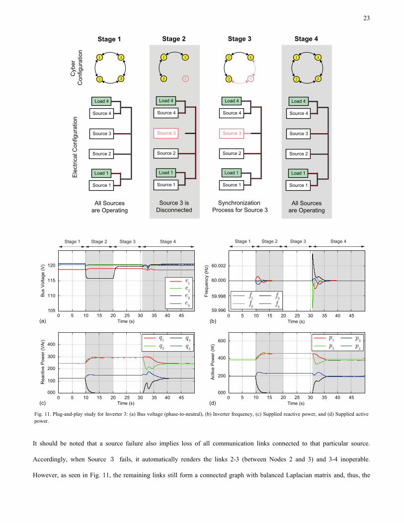
C. Plug-and-play Study
Figure 11 studies the plug-and-play capability of the proposed method. Inverter 3 has intentionally been unplugged at
10 st = . Although this inverter is turned off instantly, the power measurements exponential decay to zero because of the
existing low-pass filters.
000
10
Sup
plie
d A
ctiv
e P
ower
(W)
Time (s)
100
200
300
400
15 20 25 30 35
(a) Maximum Delay = 1 ms, Minimum Channel Bandwidth = 100 kHz
000
10
Sup
plie
d R
eact
ive
Pow
er (V
Ar)
Time (s)
100
200
300
400
15 20 25 30 35
act.1q
act.2q
act.3q
act.4q 500
600act.1p
act.2p
act.3p
act.4p
� 1 4 1 41 4
Z Z Z ZZ Z ���������������������� � 1 4 1 41 4
Z Z Z ZZ Z ����������������������
000
10S
uppl
ied
Act
ive
Pow
er (W
)Time (s)
100
200
300
400
15 20 25 30 35
(b) Maximum Delay = 50 ms, Minimum Channel Bandwidth = 10 kHz
000
10
Sup
plie
d R
eact
ive
Pow
er (V
Ar)
Time (s)
100
200
300
400
15 20 25 30 35
500
600act.1q
act.2q
act.3q
act.4q
act.1p
act.2p
act.3p
act.4p
000
10
Sup
plie
d A
ctiv
e P
ower
(W)
Time (s)
100
200
300
400
15 20 25 30 35
(c) Maximum Delay = 150 ms, Minimum Channel Bandwidth = 1 kHz
000
10
Sup
plie
d R
eact
ive
Pow
er (V
Ar)
Time (s)
100
200
300
400
15 20 25 30 35
500
600
act.1q
act.2q
act.3q
act.4q
act.1p
act.2p
act.3p
act.4p
23
Fig. 11. Plug-and-play study for Inverter 3: (a) Bus voltage (phase-to-neutral), (b) Inverter frequency, (c) Supplied reactive power, and (d) Supplied active power.
It should be noted that a source failure also implies loss of all communication links connected to that particular source.
Accordingly, when Source 3 fails, it automatically renders the links 2-3 (between Nodes 2 and 3) and 3-4 inoperable.
However, as seen in Fig. 11, the remaining links still form a connected graph with balanced Laplacian matrix and, thus, the
Time (s)
Freq
uenc
y (H
z)
(b)5 10 15 35 400 20 25 30 45
60.000
Time (s)
Bus
Vol
tage
(V)
(a)
1055 10 15 35 400 20 25 30 45
110
115
120
59.998
59.996
60.002
(c)
0005 10 15 35 400 20 25 30 45
(d) Time (s)0
Rea
ctiv
e P
ower
(VA
r)
Act
ive
Pow
er (W
)
200
400
600
Stage 1
Time (s)
1e
2e
3e
4e
3f
4f
1f
2f
Source 1
Load 1
Source 2
Source 3
Source 4
Load 4
Source 1
Load 1
Source 2
Source 3
Source 4
Load 4
Ele
ctric
al C
onfig
urat
ion
Cyb
er C
onfig
urat
ion
1 4
32
1 4
32
All Sourcesare Operating
All Sourcesare Operating
Stage 2 Stage 3 Stage 4
Stage 1 Stage 4
Stage 1 Stage 2 Stage 3 Stage 4
000
1p
2p
3p
4p
5 10 15 35 4020 25 30 45
1q
2q
3q
4q
100
200
300
400
Source 1
Load 1
Source 2
Source 3
Source 4
Load 4
1 4
32
1 4
32
Source 3 isDisconnected
Synchronization Process for Source 3
Stage 2 Stage 3
Source 1
Load 1
Source 2
Source 3
Source 4
Load 4

24
control methodology should remain functional. As seen in Figs. 11(c) and 11(d), the controllers have successfully responded to
the inverter loss and shared the excess power among the remaining inverters in proportion to their power ratings. After the loss
of Inverter 3 , the voltage measurement for Bus 3 would be unavailable. Thus, the controllers collectively regulate the new
average voltage, i.e., the average voltage of the remaining three inverters, at the rated value of 120 V . However, the actual
average voltage across the microgrid is seen to be slightly less than the rated voltage. As seen in Fig. 11(a), Bus 3
experiences voltage sag due to the loss of generation. It should be noted that although inverter 3 is disconnected from Bus 3
the bus voltage is still available. Inverter 3 is plugged back in at 20 st = ; however, the synchronization procedure delays
inverter engagement. After successful synchronization, the controller is activated at 31 st = and has shown excellent
performance in the global voltage regulation and readjusting the load sharing to account for the latest plugged-in inverter.
D. Failure Resiliency in Cyber Domain
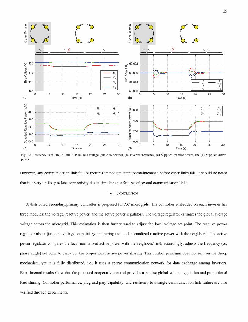
Resiliency to a single link failure is studied in Fig. 12. The original communication graph is designed to carry a minimum
redundancy, such that no single communication link failure can compromise the connectivity of the cyber network. As seen in
Fig. 12, the Link 3-4 has been disabled at 3 st = , yet, it does not have any impact on the voltage regulation or load sharing, as
the new graph is still connected and has a balanced Laplacian matrix. It should be noted that, by practicing error
detection/control protocols in the communication modules, any link failure can be immediately detected at the receiving end.
Accordingly, the receiving-end controller updates its set of neighbors by ruling out the node on the transmitting end of the
failed link. This reconfiguration ensures that the misleading zero-valued data associated to the failed link (e.g., zero active and
reactive power measurements) will not be processed by the receiving-end controller and, thus, the system remains functional.
The controller response to load change is then studied in Fig. 12 with the failed link, where a satisfactory performance is
reported. In this study, the load at Bus 4 , i.e., 4Z , has been unplugged and plugged back in at 5 st = and 17.5 st = ,
respectively. It should be noted that although the link failure does not affect the steady-state performance, it slows down the
system dynamics as it limits the information flow.
It should be noted that any reconfiguration in the cyber domain, e.g., communication link failure, affects the Laplacian
matrix and, thus, the whole system dynamic. However, it will not compromise the steady-state performance of the control
methodology, so long as the cyber network remains connected and presents a balanced Laplacian matrix. Connectivity of the
cyber network plays a key role in the functionality of the entire microgrid. Including redundant cyber links, as discussed in
sections II-A and II-B, ensures network connectivity for the most probable contingencies.
25
Fig. 12. Resiliency to failure in Link 3-4: (a) Bus voltage (phase-to-neutral), (b) Inverter frequency, (c) Supplied reactive power, and (d) Supplied active power.
However, any communication link failure requires immediate attention/maintenance before other links fail. It should be noted
that it is very unlikely to lose connectivity due to simultaneous failures of several communication links.
V. CONCLUSION
A distributed secondary/primary controller is proposed for AC microgrids. The controller embedded on each inverter has
three modules: the voltage, reactive power, and the active power regulators. The voltage regulator estimates the global average
voltage across the microgrid. This estimation is then further used to adjust the local voltage set point. The reactive power
regulator also adjusts the voltage set point by comparing the local normalized reactive power with the neighbors’. The active
power regulator compares the local normalized active power with the neighbors’ and, accordingly, adjusts the frequency (or,
phase angle) set point to carry out the proportional active power sharing. This control paradigm does not rely on the droop
mechanism, yet it is fully distributed, i.e., it uses a sparse communication network for data exchange among inverters.
Experimental results show that the proposed cooperative control provides a precise global voltage regulation and proportional
load sharing. Controller performance, plug-and-play capability, and resiliency to a single communication link failure are also
verified through experiments.
Cyb
er D
omai
n
1 4
32
Time (s)
Freq
uenc
y (H
z)
(b)0
60.000
Time (s)
Bus
Vol
tage
(V)
(a)
1055 10 150 20 25 30
110
115
120
59.998
59.996
60.002
(c)
0000
(d) Time (s)0
Sup
plie
d R
eact
ive
Pow
er (V
Ar)
Sup
plie
d A
ctiv
e P
ower
(W)
200
400
600
Time (s)
Cyb
er D
omai
n1 4
32
1 4
32
000
100
200
300
400
1e
2e
3e
4e
1 4 1 4 1 4
Z Z Z Z Z Z�����������������������
3f
4f
1f
2f
5 10 15 20 25 30
1 4
32
1 4 1 4 1 4
Z Z Z Z Z Z�����������������������
1q
2q
3q
4q
5 10 15 20 25 30
1p
2p
3p
4p
5 10 15 20 25 30

26
APPENDIX
DC bus voltages that supply the inverter modules are all dc650 VV = . The filter inductors are identical and
F1 F21.8 mHL L= = , and the intermediate capacitor is F
25 FC m= . The line impedance connecting busses i and j can be
expressed as ij ij ijZ R sL= + where,
12 12
23 23
34 34
0.8 3.6 mH
0.4 1.8 mH .
0.7 1.5 mH
R L
R L
R L
ìï = W =ïïï = W =íïïï = W =ïî
(A.1)
The control parameters are,
rated
rated
1 kW diag{1.6,1.6, 0.8, 0.8},
1 kVAr diag{0.6, 0.6, 0.3, 0.3}
ìï = ´ïïíï = ´ïïî
p
q
(A.2)
0 1 0 1
1 0 1 01.5 ,
0 1 0 1
1 0 1 0
é ùê úê úê ú= ´ ê úê úê úê úë û
GA
(A.3)
2, 0.02,b c= = (A.4)
P 4 I 4
P 4 I 4
0.01 , 3.
0.005 , 2
ìï = ´ = ´ïïíï = ´ = ´ïïî
G I G I
H I H I
(A.5)
REFERENCES
[1] J. M. Guerrero, J. C. Vasquez, J. Matas, L. G. de Vincuña, and M. Castilla, “Hierarchical control of droop-controlled ac and dc microgrids – A general approach toward standardization,” IEEE Trans. Ind. Electron., vol. 58, pp. 158–172, Jan. 2011.
[2] R. Majumder, B. Chaudhuri, A. Ghosh, R. Majumder, G. Ledwich, and F. Zare, “Improvement of stability and load sharing in an autonomous Microgrid using supplementary droop control loop,” IEEE Trans. Power Syst., vol. 25, no. 2, pp. 796–808, May 2010.
[3] H. Kakigano, Y. Miura, and T. Ise, “Distribution voltage control for dc Microgrids using fuzzy control and gain-scheduling technique,” IEEE Trans. Power Electron., vol. 28, no. 5, pp. 2246–2258, May 2013.
[4] I. U. Nutkani, P. C. Loh, P. Wang, and F. Blaabjerg, “Cost-prioritized droop schemes for autonomous ac microgrids,” IEEE Trans. Power Electron., vol. 30, no. 2, pp. 1109–1119, Feb. 2015.
[5] P. C. Loh, D. Li; Y. K. Chai, and F. Blaabjerg, “Autonomous operation of hybrid microgrid with ac and dc subgrids,” IEEE Trans. Power Electron., vol. 28, no. 5, pp. 2214–2223, May 2013.
[6] M. Datta, T. Senjyu, A. Yona, T. Funabashi, and C. H. Kim, “A frequency-control approach by photovoltaic generator in a PV-diesel hybrid power system,” IEEE Trans. Energy Convers., vol. 26, no. 2, pp. 559–571, Jun. 2011.
[7] C. K. Sao and W. Lehn, “Control and power management of converter-fed microgrids,” IEEE Trans. Power Syst., vol. 23, pp. 1088–1098, Aug. 2008. [8] E. Serban and H. Serban, “A control strategy for a distributed power generation microgrid application with voltage- and current-controlled source
converter,” IEEE Trans. Power Electron., vol. 15, pp. 2981–2992, Dec. 2010. [9] A. Bidram and A. Davoudi, “Hierarchical structure of microgrids control system,” IEEE Trans. Smart Grid, vol. 3, pp. 1963–1976, Dec 2012. [10] J. C. Vasquez, J. M. Guerrero, J. Miret, M. Castilla, and L.G. de Vicuña, “Hierarchical control of intelligent microgrids,” IEEE Ind. Electron. Mag., vol.
4, pp. 23–29, Dec. 2010. [11] J. A. P. Lopes, C. L. Moreira, and A. G. Madureira, “Defining control strategies for microgrids islanded operation,” IEEE Trans. Power Syst., vol. 21,
pp. 916–924, May 2006. [12] F. Katiraei, M. R. Iravani, and P. W. Lehn, “Microgrid autonomous operation during and subsequent to islanding process,” IEEE Trans. Power Del., vol.
20, pp. 248–257, Jan. 2005. [13] M. Savaghebi, A. Jalilian, J. Vasquez, and J. Guerrero, “Secondary control for voltage quality enhancement in microgrids,” IEEE Trans. Smart Grid, vol.
3, pp. 1893–1902, Dec. 2012. [14] H. Kanchev, D. Lu, F. Colas, V. Lazarov, and B. Francois, “Energy management and operational planning of a microgrid with a PV-based active
generator for smart grid applications,” IEEE Trans. Ind. Electron., vol. 58, no. 10, pp. 4583–4592, Oct. 2011. [15] C. Chen, S. Duan, T. Cai, B. Liu, and G. Hu, “Optimal allocation and economic analysis of energy storage system in microgrids,” IEEE Trans. Power
Electron., vol. 26, no. 10, pp. 2762–2773, Oct. 2011. [16] N. Ainsworth and S. Grijalva, “A structure-preserving model and sufficient condition of frequency synchronization of lossless droop inverter-based ac
network,” IEEE Trans. Power Syst., vol. 28, pp. 4310–4319, Nov. 2013. [17] D. Wu, F. Tang, J. M. Guerrero, and J. C. Vasquez, “Autonomous control of distributed generation and storage to coordinate P/Q sharing in islanded
microgrids – An approach beyond droop control,” in Proc. IEEE Int. Energy Conf., 2014, pp. 983–988.
27
[18] J. Y. Kim, J. H. Jeon, S. K. Kim, C. Cho, J. H. Park, H. M. Kim, and K. Y. Nam, “Cooperative control strategy of energy storage system and micro sources for stabilizing the microgrid during islanded operation,” IEEE Trans. Power Electron., vol. 25, pp. 3037–3048, Dec. 2010.
[19] S. M. Ashabani and Y. A. R. I. Mohamed, “General interface for power management of micro-grids using nonlinear cooperative droop control,” IEEE Trans. Power Syst., vol. 28, pp. 2929–2941, Aug. 2013.
[20] J. Hu, J. Zhu, D. G. Dorrell, and J. M. Guerrero, “Virtual flux droop method – A new control strategy of inverters in microgrids,” IEEE Trans. Power Electron., vol. 29, pp. 4704–4711, Sept. 2014.
[21] Y. A. I. Mohamed and E. F. El-Saadany, “Adaptive decentralized droop controller to preserve power sharing stability of paralleled inveretrs in distributed generation microgrids,” IEEE Trans. Power Electronics, vol. 23, pp. 2806–2816, Nov. 2008.
[22] J. He and Y. W. Li, “Analysis, design, and implementation of virtual impedance for power electronics interfaced distributed generation,” IEEE Trans. Ind. Appl., vol. 41, pp. 2525–2538, Nov./Dec. 2011.
[23] J. W. Simpson-Porco, F. Dorfler, and F. Bullo, “Voltage stabilization in microgrids via quadratic droop control,” IEEE 52nd Annu. Conf. Decision and Control, 2013, pp. 7582–7589.
[24] H. Mahmood, D. Michaelson, and J. Jiang, “Accurate reactive power sharing in an islanded microgrid using adaptive virtual impedances,” IEEE Trans. Power Electron., vol. 30, no. 3, pp. 1605–1617, Mar. 2015.
[25] H. Han, Y. Liu, Y. Sun, M. Su, and J. M. Guerrero, “An improved droop control strategy for reactive power sharing in islanded microgrid,” IEEE Trans. Power Electron., vol. 30, no. 6, pp. 3133–3141, Jun. 2015.
[26] J. Rocabert, A. Luna, F. Blaabjerg, and P. Rodriguez, “Control of power converters in ac microgrids,” IEEE Trans. Power Electron., vol. 27, pp. 4734–4749, Nov. 2012.
[27] C. T. Lee, C. C. Chu, and P. T. Cheng, “A new droop control method for the autonomous operation for distribute energy resource interface converters,” IEEE Trans. Power Electron., vol. 28, pp. 1980–1993, Apr. 2013.
[28] S. V. Dhople. B. B. Johnson, and A. O. Hamadeh, “Virtual oscillator control for voltage source inverters,” in Proc. 51st Annu. Allerton Conf., 2013, pp. 1359–1363.
[29] B. B. Johnson, S. V. Dhople. A. O. Hamadeh, and P. T. Krein, “Synchronization of nonlinear oscillators in an LTI electrical power network,” IEEE Trans. Circuits Syst. I: Reg. Papers, vol. 61, pp. 834–844, Mar. 2014.
[30] B. B. Johnson, S. V. Dhople. A. O. Hamadeh, and P. T. Krein, “Synchronization of parallel single-phase inverters with virtual oscillator control,” IEEE Trans. Power Electron., vol. 29, no. 11, pp. 6124–6138, Nov. 2014.
[31] B. B. Johnson, S. V. Dhople, J. L. Cale, A. O. Hamadeh, and P. T. Krein, “Oscillator-based inverter control for islanded three-phase microgrids,” IEEE J. Photovoltaics, vol. 4, no. 1, pp. 387–395, Jan. 2014.
[32] T. L. Vandon, B. Meersman, J. D. M. De Koonig, and L. Vandevelde, “Analogy between conventional grid control and islanded microgrid control based on a global dc-link voltage droop,” IEEE Trans. Power Del., vol. 27, pp. 1405–1414, July 2012.
[33] A. H. Etemadi, E. J. Davison, R. Iravani, “A decentralized robust strategy for multi-DER microgrids – Part I: Fundamental concepts,” IEEE Trans. Power Del., vol. 27, pp. 1843–1853, Oct. 2012.
[34] Q. Shafiee, V. Nasirian, J. M. Guerrero, F. L. Lewis, and A. Davoudi, “Team-oriented adaptive droop control for autonomous AC microgrids,” in Proc. 40th Ind. Electron. Conf. (IECON), 2014, pp. 1861–1867.
[35] A. Micallef, M. Apap, C. Spiteri-Staines, J. M. Guerrero, and J. C. Vasquez, “Reactive power sharing and voltage harmonic distortion compensation of droop controlled single phase islanded microgrids,” IEEE Trans. Smart Grid, vol. 5, pp. 1149–1158, May 2014.
[36] A. Mehrizi-Sani and R. Iravani, “Potential-function based control of a microgrid in islanded and grid-connected modes,” IEEE Trans. Power Syst., vol. 25, pp. 1883–1891, Nov. 2010.
[37] A. Mehrizi-sani and R. Iravani, “Constrained potential function-based control of microgrids for improved dynamic performance,” IEEE Trans. Smart Grid, vol. 3, pp. 1885–1892, Dec. 2012.
[38] A. H. Etemadi, E. J. Davison, R. Iravani, “A decentralized robust strategy for multi-DER microgrids – Part II: Performance evaluation,” IEEE Trans. Power Del., vol. 27, pp. 1854–1861, Oct. 2012.
[39] A. H. Etemadi, E. J. Davison, R. Iravani, “A generalized decentralized robust control of islanded microgrids,” IEEE Trans. Power Syst., vol. 29, no. 6, pp. 3102–3113, Nov. 2014.
[40] A. Kahrobaeian and Y. A. R. I. Mohamed, “Networked-based hybrid distributed power sharing and control of islanded micro-grid systems,” IEEE Trans. Power Electron., vol. 30, no. 2, pp. 603–617, Feb. 2015.
[41] Q. Hui and W. Haddad, “Distributed nonlinear control algorithms for network consensus,” Automatica, vol. 42, pp. 2375–2381, Sept. 2008. [42] J. Fax and R. Murray, “Information flow and cooperative control of vehicle formations,” IEEE Trans. Automat. Control, vol. 49, pp. 1465–1476, Sept.
2004. [43] Z. Qu, Cooperative control of dynamical systems: Applications to autonomous vehicles. New York: Springer-Verlag, 2009. [44] Q. Shafiee, J. M. Guerrero, and J. C. Vasquez, “Distributed secondary control for islanded microgrids – A novel approach,” IEEE Trans. Power
Electron., vol. 29, pp. 1018–1031, Feb. 2014. [45] Q. Shafiee, C. Stefanovic, T. Dragicevic, P. Popovski, J. C. Vasquez, and J. M. Guerrero, “Robust networked control scheme for distributed secondary
control of islanded microgrids,” IEEE Trans. Ind. Electron., vol. 61, pp. 5363–5374, Oct. 2014. [46] Y. Zhang and H. Ma, “Theoretical and experimental investigation of networked control for parallel operation of inverters,” IEEE Trans. Ind. Electron.,
vol. 59, pp. 1961–1970, Apr. 2012. [47] M. N. Marwali and A. Keyhani, “Control of distributed generation systems – Part I: Voltages and currents control,” IEEE Trans. Power Electron., vol.
19, pp. 1541–1550, Nov. 2004. [48] M. N. Marwali, J. W. Jung, and A. Keyhani, “Stability analysis of load sharing control for distributed generation systems,” IEEE Trans. Energy
Convers., vol. 22, pp. 737–745, Sept. 2004. [49] S. D. J. McArthur, E. M. Davidson, V. M. Catterson, A. L. Dimeas, N. D. Hatziargyriou, F. Ponci, and T. Funabashi, “Multi-agent systems for power
engineering applications – part I: Concepts, approaches, and technical challenges,” IEEE Trans. Power Syst., vol. 22, pp. 1743–1752, Nov. 2007. [50] A. Bidram, A. Davoudi, and F. L. Lewis, “A multi-objective distributed control framework for islanded microgrids,” IEEE Trans. Ind. Informatics, vol.
10, no. 3, pp. 1785–1798, Aug. 2014. [51] A. Bidram, A. Davoudi, F. L. Lewis, and Z. Qu, “Secondary control of microgrids based on distributed cooperative control of multi-agent systems,” IET
Generation, Transmission Dist., vol. 7, pp. 822–831, Aug. 2013. [52] V. Nasirian, A. Davoudi, and F. L. Lewis, “Distributed adaptive droop control for dc microgrids,” in Proc. 29th IEEE Appl. Power Electron. Conf. Expo.
(APEC), 2014, pp. 1147–1152. [53] V. Nasirian, S. Moayedi, A. Davoudi, and F. L. Lewis, “Distributed cooperative control of dc microgrids,” IEEE Trans. Power Electron., vol. 30, pp.
2288–2303, Apr. 2015. [54] V. Nasirian, A. Davoudi, F. L. Lewis, and J. M. Guerrero, “Distributed adaptive droop control for dc distribution systems,” IEEE Trans. Energy
Convers., vol. 29, pp. 944–956, Dec. 2014. [55] S. Moayedi, V. Nasirian, F. L. Lewis, and A. Davoudi, “Team-oriented load sharing in parallel dc-dc converters,” IEEE Trans. Ind. Appl., vol. 51, no. 1,
pp. 479–490, Jan./Feb. 2015.
28
[56] B. A. Robbins, C. N. Hadjicostis, and A. D. Dominguez-Garcia, “A two-stage distributed architecture for voltage control in power distribution systems,” IEEE Trans. Power Syst., vol. 28, pp. 1470–1482, May 2013.
[57] A. D. Dominguez-Garcia, C. N. Hadjicostis, and N. F. Vaidya, “Resilient networked control of distributed energy resources,” IEEE J. Sel. Areas Commun., vol. 30, pp. 113–1148, Jul. 2012.
[58] S. T. Cady and A. D. Dominguez-Garcia, “Distributed generation control of small-footprint power systems,” in Proc. North American Power Symp., 2012, pp. 1–6.
[59] F. Dorfler,J. W. Simpson-Porco, and F. Bullo, “Breaking the hierarchy: Distributed control and economic optimality in microgrids,” 2014, Available on arXiv:1401.1767v1.
[60] H. Bouattour, J. W. Simpson-Porco, F. Dorfler, and F. Bullo, “Further results on distribute secondary control in microgrids,” IEEE Conf. on Decision and Control, 2013, pp.1514–1519.
[61] J. W. Simpson-Porco, F. Dorfler, F. Bullo, Q. Shafiee, and J. M. Guerrero, “Stability, power sharing, and distributed secondary control in droop-controlled microgrids,” IEEE Smart Grid Commun. Symp., 2013, pp. 672–677.
[62] J. W. Simpson-Porco, F. Dorfler, and F. Bullo, “Synchronization and power sharing for droop-controlled inverters in islanded microgrids,” Automatica, vol. 49, pp. 2603–2611, Jun. 2013.
[63] R. Olfati-saber, J. A. Fax, and R. M. Murray, “Consensus and cooperation in networked multi-agent systems,” Proc. IEEE, vol. 95, no. 1, pp. 215–233, Jan. 2007.
[64] R. Olfati-Saber and R. M. Murray, “Consensus problems in networks of agents with switching topology and time-delays,” IEEE Trans. Automat. Control, vol. 49, no. 9, pp. 1520–1533, Sept. 2004.
[65] R. W. Erickson and D. Maksimovic, Fundamental of Power Electronics, 2nd Ed. Norwell, MA: Kluwer, 2001. [66] D. P. Spanos, R. Olfati-Saber, and R. M. Murray, “Dynamic consensus for mobile networks,” in Proc. 16th Int’l. Fed. Automat. Control (IFAC), 2005,
pp. 1–6. [67] L. Chen, C. Hu, Q. Zhang, K. Zhang, and I. Batarseh, “Modeling and triple-loop control of ZVS grid-connected dc/ac converters for three-phase
balanced micro-inverter application,” IEEE Trans. Power Electron, vol. 30, No. 4, pp. 2010–2023, Apr. 2015. [68] Y. Sozer and D. A. Torrey, “Modeling and control of utility interactive inverters,” IEEE Trans. Power Electron., vol. 24, no. 11, pp. 2475–2483, Nov.
2009. [69] N. Pogaku, M. Prodanovic, and T. C. Green, “Modeling, analysis and testing of autonomous operation of an inverter-based microgrid,” IEEE Trans.
Power Electron., vol. 22, no. 2, pp. 613–625, Mar. 2007. [70] X. Guo, Z. Lu, B. Wang, X. Sun, L. Wang, and J. M. Guerrero, “Dynamic phasors-based modeling and stability analysis of droop-controlled inverters for
microgrid applications,” IEEE Trans. Smart Grid, vol. 5, no. 6, pp. 2980–2987, Nov. 2014. [71] H. Zhang, F. L. Lewis, and Z. Qu, “Lyapunov, adaptive, and optimal design techniques for cooperative systems on directed communication graphs,”
IEEE Trans. Ind. Electron., vol. 59, no. 7, pp. 3026–3041, Jul. 2012. [72] F. Xiao and L. Wang, “Asynchronous consensus in continuous-time multi-agent systems with switching topology and time-varying delays,” IEEE Trans.
Automat. Control, vol. 53, no. 8, pp. 1804–1816, Sept. 2008. [73] S. Ci, J. Qian, D. Wu, and A. Keyhani, “Impact of wireless communication delay on load sharing among distributed generation systems through smart
microgrids,” IEEE Wireless Communications, vol. 19, no. 3, pp. 24–29, Jun. 2012. [74] S. Liu, X. Wang, and P. X. Liu, “Impact of communication delays on secondary frequency control in an islanded microgrid,” IEEE Trans. Ind. Electron.,
to be published, DOI: 10.1109/TIE.2014.2367456. [75] H. Behjati, A. Davoudi, and F. L. Lewis, “Modular DC-DC converters on graphs: cooperative control,” IEEE Trans. Power Electron., vol. 29, no. 12, pp.
6725–6741, Dec. 2014.


