
1
Abstract—Multi-view/3D video is currently available in
games, entertainment, education, security, and surveillance
applications. Since the amount of data in multi-view/3D
increases proportionally with the number of cameras, and due
to different bandwidth and playback capabilities of receivers,
appropriate compression of multi-view/3D video to produce the
correct bitrate while maintaining smooth video quality is
crucial; a task that is mostly performed by the Rate Control
module of the encoder. There are many existing rate control
algorithms for single-view and multi-view video coding
considering the specific features or aspects of these videos. In
this paper, we introduce a novel view-level Rate Distortion
(RD) model. We use a systematic methodology to derive this
RD model by investigating the impact of multi-view/3D video
characteristics on the bitrate of a compressed video. Our
proposed RD model considers the concepts of intra-view and
inter-view disparity as an effective feature of multi-view/3D
video to estimate the overall bitrate of each view more
accurately. Evaluation results indicate that our proposed view-
level RD model outperforms existing linear models by a factor
of 3 and can predict the rate of each view with relatively high
precision and a low estimation error of 12% on average.
Index Terms— Inter-view disparity, intra-view disparity,
multi-view video coding, rate control.
I. INTRODUCTION
ulti-view/3D video provides viewers with a more
realistic experience by interactively changing the
view-points that are captured with the help of
multiple cameras from different positions and through
different angles. Stereo video, as the first generation of 3D
video, provides two distinct views, one for each eye. But 3D
video as the second generation attempts to overcome one of
the disadvantages of conventional stereo video: its
restriction to two views at fixed spatial positions [1]. In
immersive video communication applications, such as free
viewpoint and 3D television, the amount of data increases
proportionally with the number of cameras, which may limit
H. Roodaki is with the Multimedia Processing Laboratory, School of
Electrical and Computer Engineering, College of Engineering, University
of Tehran, Tehran, Iran (e-mail: [email protected]). Z. Iravani is with the Multimedia Processing Laboratory, School of
Electrical and Computer Engineering, College of Engineering, University
of Tehran, Tehran, Iran (e-mail: [email protected]). M.R. Hashemi is with the Multimedia Processing Laboratory, School of
Electrical and Computer Engineering, College of Engineering, University
of Tehran, Tehran, Iran (e-mail: [email protected]). S. Shirmohammadi is with the Multimedia Processing Laboratory,
School of Electrical and Computer Engineering, College of Engineering,
University of Tehran, Tehran, Iran (e-mail: [email protected]) and the Distributed and Collaborative Virtual Environments Research
Laboratory, School of Electrical Engineering and Computer Science,
Faculty of Engineering, University of Ottawa, Ottawa, Canada (e-mail: [email protected]).
the practicality of multi-view/3D video especially when
receivers have limited bandwidth. Hence, having an
appropriate bit allocation method to adapt the video rate to
available resources is one of the main challenges in Multi-
view Video Coding (MVC). This bit allocation is performed
by the Rate Control Algorithm (RCA), which plays an
important role in improving and stabilizing the perceived
quality at a given bitrate.
Several RCAs have been proposed for MVC that usually
utilize a Rate-Distortion (RD) model to describe the
relationship between the rate and the quality of the encoded
video. For a rate control algorithm, the RD model is a key
part since its accuracy greatly affects the rate control
performance.
There are two principal methods to obtain an RD model:
statistical and experimental [2]. Statistical models assume
that the source signal has a specific distribution such as
Gaussian distribution. Most existing RD models for MVC
are statistical models that have a common base theory, but
differ in the way they have simplified the model or the
various assumptions they have made to make it more
practical. Several of these methods will be reviewed in the
next section. Statistical models are not as accurate as
experimental models since they use a single model for all
data. Finding accurate statistical RD models are only
available for very simple sources under specific criteria.
On the other hand, experimental models consider the RD
characteristics of input data, and hence can provide a more
accurate RD curve [2]. They can be dynamically updated
through a data fitting process to provide higher prediction
accuracy. However, existing experimental RD models for
MVC in the literature have some drawbacks. They do not
explicitly consider the characteristics or the encoding
structure and parameters of multi-view/3D sources. Hence,
their obtained RD performance is limited.
In this paper, we go beyond existing literature and derive
a novel and efficient experimental RD model for multi-view
video coding that specifically considers the characteristic of
multi-view/3D sources. Usually, MVC rate control
algorithms are designed for different levels such as view-
level, GOP-level, frame-level, etc. This way, at each level
the most effective parameters of that level can be used to
estimate the rate more accurately. In addition, the approach
can manage the required memory capacity and
computational complexity of the rate control algorithm.
Similarly, our proposed scheme considers the rate allocation
process at the view-level because, as we shall see later, the
specific characteristics of multi-view/3D video, namely
inter-view and intra-view disparity [29], are mostly reflected
at this level. Our proposed approach can indeed be
generalized easily to the other levels too. The main
contributions of this paper are as follows:
Our extracted RD model uses the statistical
A View-level Rate-Distortion Model for Multi-
view/3D Video
H. Roodaki, Z. Iravani, M.R. Hashemi, and S. Shirmohammadi
M
2
dependencies within the multi-view frames as the
main characteristic of multi-view/3D video, to find
the RD model parameters. This is important since
these statistical dependencies, which are the disparity
between views and motion between temporally
successive frames, can affect the prediction process
and therefore the total bitrate of each view
considerably.
Our proposed model uses the concepts of intra-view
and inter-view disparity to characterize the statistical
dependencies in multi-view video coding. Then, it
defines the rate of each view as a function of these
intra and inter-view disparity.
We have used a systematic approach to derive the
proposed experimental view-level RD model
parameters considering the main characteristics of
multi-view/3D video and the application at hand. We
show that reflecting these features in the RD model
results in a more accurate view-level RD model.
Since the proposed RD model extraction
methodology considers the properties of the specific
application, the extracted RD model can be easily
tuned for a wide range of multi-view/3D video
applications.
Although our proposed approach considers the
H.264/MVC standard and its applications to find the
proper RD parameters, it can be easily generalized to
other video compression standards such as the 3D and
multi-view extensions of the emerging HEVC standard,
once the appropriate RD parameters are selected
according to that standard.
The rest of this paper is organized as follows. Related
multi-view rate models and their corresponding rate
control algorithms are reviewed in the next section. The
proposed methodology to derive the view-level RD model
is explained in section III. Section IV presents the derived
view-level RD model for the H.264/AVC by applying this
systematic methodology. Section V provides the
performance evaluation results. Finally, the paper ends in
section VI with the concluding remarks.
II. RELATED WORK
As mentioned in the previous section, most of the
proposed rate control algorithms use some kind of rate-
distortion model to describe the relationship between rate
and quality. A quadratic rate-distortion model for rate
control of MVC is introduced in [3] that consists of three
levels for more accurate bitrate control: group of GOP,
GOP, and frame. The rate-distortion model for multi-view
video proposed in [4] argues that the quality of each view
follows an increasing logarithmic function of the view
encoding rate. In [5] the authors argue that the traditional
video compression methods do not address the perception
redundancy. This paper introduces a just-noticeable-
distortion (JND) model in MVC to describe the perception
redundancy quantitatively. An analytical model for rate-
distortion analysis in multi-view image coding is proposed
in [6] in which the images are predicted using the disparity
compensation based on depth map. A rate-distortion model
to characterize the relationship between bitrate and view
synthesis distortion is derived in [7]. Then, the optimal
bitrate is allocated to texture and depth using this model.
The interdependent distortion-quantization model and rate-
quantization model is proposed in [8]. The proposed models
are based on the analysis of the relationship between the
spatial-domain residual and the transform-domain residual.
In [9], a spatially scalable rate-distortion model is proposed
that consists of quantization-distortion and quantization-rate
models.
In addition to the above RD models, some rate control
algorithms are proposed for multi-view video coding.
In [10], an MVC rate control algorithm based on the
quadratic rate-distortion and the fluid-flow traffic model is
proposed. A view-level bitrate estimation technique for real-
time multi-view video plus depth is introduced in [11] that is
based on statistical analysis of the prediction modes used in
different view types. In [12], the authors argue that MVC
has many B views which are composed of only B frames.
Hence, they propose to consider the QP values of B frames
to allocate proper bitrates to B views. A rate control method
is proposed in [13] that utilizes the human visual system to
distribute bitrate to interesting and non-interesting regions of
a frame. A rate control technique for multi-view video plus
depth is introduced in [14] that is performed on three levels:
view level, video/depth level and frame level. In [15], a rate
control algorithm for MVC is proposed that remodels the
quadratic RD model based on the type of each frame.
Another three level rate control algorithm is proposed
in [16] that allocates rate at view level, GOP level and frame
level. In this method, the rate allocation is done according to
view types using a pre-statistical rate allocation method and
considering the complexity of each frame. In [17], a rate
control algorithm for MVC is proposed that uses a bit
allocation model based on the Lagrange theorem. A rate
controller for MVC is presented in [18] that exploits inter-
GOP correlations to predict the bitrate of future frames
considering the intra-GOP linearity. In [19], the authors
propose a new rate control algorithm for multi-view video
reference model using the quadratic RD model that consists
of four levels for bitrate control. The characteristics of
visual perception for 3D video viewers is utilized in [20] to
determine the interesting regions in all views. Then the
adequate quantization parameters are assigned to control the
bitrate of these interesting and non-interesting regions such
that the video quality of the interesting regions is preserved.
In [21], a rate control algorithm for multi-view video coding
is proposed based on visual perception. This algorithm
consists of four levels. In the view level, a GOP is pre-
encoded to obtain the bitrates proportion among the views.
The initial quantization parameter and the target bits are
calculated for the GOP at the GOP level. The complexity of
the frame is used for bit allocation at the frame level. As a
final point, at the macro-block level, the rate distortion
model is adjusted based on the visual perception. Finally,
in [22] a novel hierarchical rate control for multi-view video
coding is presented that addresses the rate control at both
frame level and basic unit level.
Despite the benefits of the above approaches, they have a
one-solution-fits-all mentality. None of them has considered
the statistical dependencies within the multi-view frames as
the main characteristic of MVC that affects the effectiveness
of the prediction process considerably. In addition, the
features related to the application such as quality of
experience are not considered in the previous methods.
These must be taken into account for higher efficiency. In
our approach, we will introduce a novel view-level RD

3
model for different applications of MVC using the specific
features of multi-view/3D video format and the application
at hand. This way, the derived RD model can be applied
more precisely to a practical situation of multi-view/3D
video.
III. METODOLOGY STEPS
We have used a systematic methodology to derive our
proposed view-level RD model. In this section, we introduce
the different steps of this methodology in details. We start
by explaining the basic observations that have led to our
methodology.
A. Observations
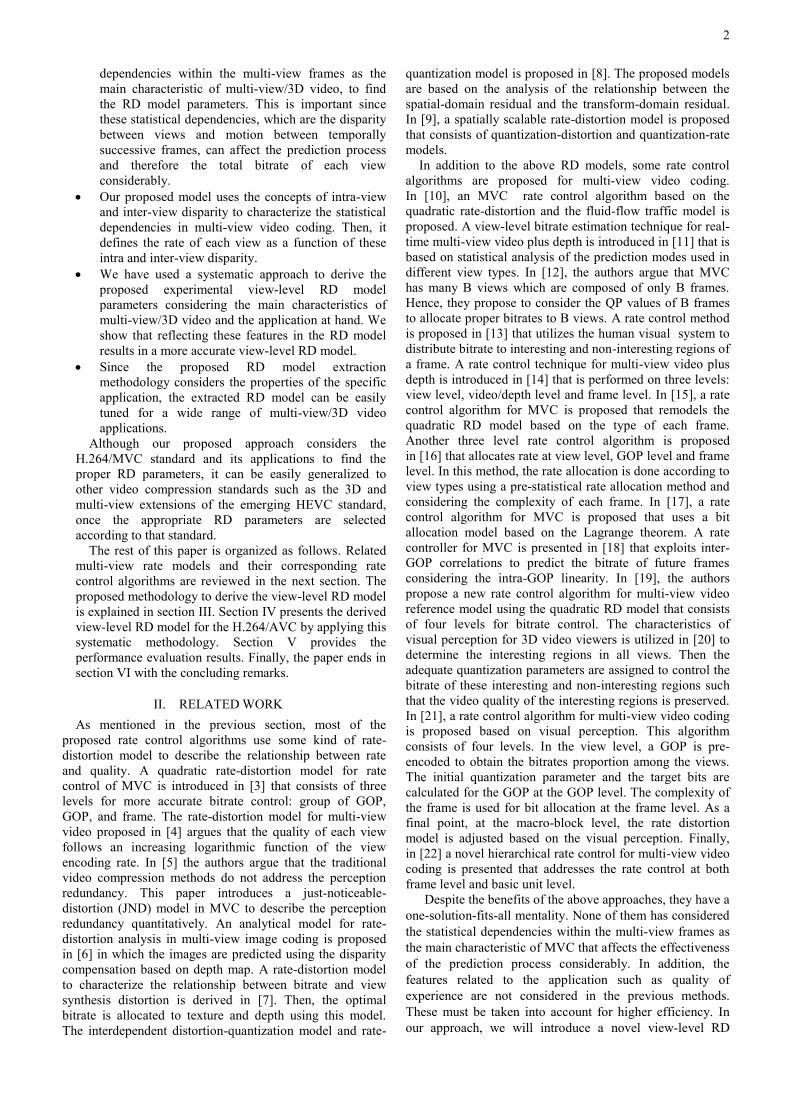
A typical MVC prediction structure proposed by the
H.264/MVC standard is shown in Fig 1[23].
Fig 1. A typical MVC prediction structure [23]
Apart from the temporal redundancy between consecutive
frames, spatial redundancy between frames of neighboring
views in the prediction structure can also be exploited to
increase the compression ratio. Motion and disparity
compensated coding techniques are used for this purpose.
Motion compensation exploits the temporal correlation
within each view, and disparity compensation exploits the
correlation among multiple view sequences. Motion and
disparity vectors are selected based on the rate-distortion
criterion which minimizes the rate subject to a constraint on
overall distortion. Hence, the rate of each view can be
affected considerably by the correlation between
neighboring views of the prediction structure, and the
correlation between the consecutive frames of each view.
Accordingly, we suggest that the bitrate of each view should
be a function of intra-view and inter-view disparity indicator
parameters as represented in (1):
R = F(Intra − view disparity indicator paremeters , Inter −view disparity indicator parameters) (1)
where R denotes the bitrate of each view and F represents
the relationship between that bitrate, inter-view and intra-
view disparity related parameters.
Hence, it follows that a method to derive appropriate
view-level RD model should consist of three steps, as
illustrated in Fig 2 and described in more details in sub-
sections B, C and D respectively.
B. Step 1: Extracting intra-view RD model
1) Extract the effective parameters to characterize
intra-view disparity
Fig 2. The overall structure of our proposed methodology to derive view-
level RD model for multi-view/3D video
As mentioned above, motion compensation exploits the
temporal correlation within the frames of each view. Hence,
the prediction process and consequently the rate of each
view can be affected considerably by the correlation
between the consecutive frames of each view. This
correlation depends on various parameters such as the GOP
length, the number of reference picture for each frame, the
video content complexity and so on. In order to find the
effective parameters to characterize the intra-view disparity,
our proposed methodology suggests finding the most
important parameters that affect the intra-view prediction
process.
2) Derive the relationship between the bitrate of each
view and the intra-view disparity indicator
parameters
Now, the relationship between the overall bitrate of each
view and the related parameter to intra-view disparity
should be extracted. We suggest an analytical approach
using curve fitting for this purpose, explained in details in
section IV. Using this approach, we obtain an RD model
that shows the relationship between the total bitrate of each
view and the intra-view indicator parameters.
C. Step 2: Extracting inter-view RD model
1) Extract the effective parameters to characterize
inter-view disparity
As mentioned before, in addition to the temporal
redundancy between successive frames, spatial redundancy
between frames of neighboring views in the prediction
structure can affect the efficiency of the prediction process
and the overall bitrate of each view. So, similar to the
previous step, we should characterize the inter-view
disparity and find the corresponding effective parameters.
2) Derive the relationship between the bitrate of each
view and the inter-view disparity indicator
parameters
Similar to the previous step, at this point, the relationship
between the overall bitrate of each view and the related
parameter to inter-view disparity should be extracted
analytically via curve fitting.
This way, at the end of this step, we obtain an RD model
that shows the relationship between the total bitrate of each
view and the inter-view disparity indicator parameters.

4
D. Step 3: General view-level RD model for Multi-
view/3D video
As the last step of our proposed methodology, the two
extracted RD models in the previous steps should be
combined to derive the general view-level RD model for
multi-view video.
As we can see in the prediction structure of Fig 1,
different views of a multi-view video use the intra-view and
inter-view prediction to improve the coding efficiency. In
addition, as we explained in subsection A, the motion and
disparity vectors that are extracted from intra and inter-view
predictions are completely independent from each other.
Hence, we can consider the final view-level RD model for
multi-view/3D video as the weighted sum of two RD models
extracted from intra-view and inter-view related parameters.
As explained below, in this paper the ratio between the
number of intra and inter-view predictions in each view
determines the proper weigh values.
Simulation results for various videos show that for
those views which have one reference view for inter-view
prediction, such as V2 in Fig 1, the number of inter-view
predictions is much less than intra-view predictions.
Similarly, the ratio of inter-view prediction to intra-view
prediction in views with two inter-view references, such as
V1 in Fig 1, is much higher. Clearly, when the number of
inter-view prediction increases, the importance of inter-view
disparity in determining the final bitrate will increase as
well. Hence, the ratio of inter-view and intra-view
predictions can be used to calculate the appropriate weight
values for our final view-level RD model.
IV. EXTRACTING THE VIEW-LEVEL RD MODEL FOR MULTI-
VIEW/3D VIDEOS
In this section we will apply the three steps of the
proposed methodology to extract an experimental view-level
RD model for multi-view/3D videos. The details of the
procedure are described in the following subsections.
A. Step 1: Extracting intra-view RD model
1) Extract the effective parameters to characterize
intra-view disparity
As explained in the first step of the proposed
methodology, in order to find the effective parameters to
characterize the intra-view disparity, the most important
parameters that affect the bitrate of each view should be
extracted.
In [24], a method to select the most effective parameters
in the bitrate of each view in multi-view/3D video is
introduced. According to this study, we should collect and
categorize all of the encoding parameters and features that
affect the bitrate and the perceptual quality of multi-
view/3D video during the prediction process according to
the H.264/MVC standard. The effect of each encoding
parameter and feature in the overall bitrate of each view is
determined by changing only that parameter or feature in the
encoding process and considering the rest as fixed. The
encoding parameters and feature that do not have a
significant impact on overall bitrate of each view are
discarded from the list of parameters. This approach found
that among the related parameters, the “video content
complexity” concept has the most important effect on the
bitrate of each view [24]. Hence, based on the outcome of
this study, we will use this concept to characterize the
impact of intra-view disparity in the prediction process and
the total bitrate of each view.
2) Derive the relationship between the rate of each
view and the intra-view disparity indicator
parameters
According to the methodology, at this point the
relationship between the bitrate of each view and the video
content complexity concept should be derived.
For this purpose, we should parameterize the video
content complexity concept by defining the appropriate
parameters that describe it. Several methods have been
introduced in the literature to parameterize this concept. In
this paper and similar to [24], we have used the “scene
complexity” and “level of motion” parameters to
characterize the video content complexity concept. Using
these parameters has some advantages. They can be
calculated using the codec related variables which are
already calculated in the encoding process. Hence, this
calculation has a minimal cost compared to calculating the
content complexity directly from the pixel values of the
uncompressed frames. Although complexity reduction can
decrease the accuracy of calculations, but the results of our
experiments show that using these parameters provides
acceptable accuracy. It should be noted that the selected
parameters represent just an example to explain the steps of
our methodology, and the proposed methodology can be
used with any other related parameters.
The “scene complexity” and “level of motion” parameters
are defined in [24] as follows:
Scene Complexity(C) = BitrateI
2×106×0.89QPI (2)
Level of Motion(M) = BitrateP+BitrateB
2×106×0.89(QPP+QPB) (3)
where BitrateI, BitrateP and BitrateB are the number of bits
that are used for I, P and B frames and QPI, QPP and QPB are
the average quantization parameters of I, P and B frames,
respectively. The constant values in these equations are
selected as follows. A total of 52 values of quantization step
sizes are supported in the H.264/AVC standard that are
indexed by QPs. The value of the quantization steps are
arranged in a way that an increase of 6 in QP means
doubling the quantization step size. Hence, an increase of 1
in QP corresponds to a reduction of bitrate by approximately
1 −1
2
1
6 = 0.89 [24].
Now we can extract the relationship between the total
bitrate of each view and the concept of video content
complexity using C and M parameters. The details of this
procedure are as follows.
Theoretically, the coding complexity function is defined
as the multiplication of QS and the required bit budget for
encoding [26]:
Coding Complexity = QP × R (4)
On the other hand, as we explained before, the coding
complexity is defined as a function of C and M parameters.
Coding Complexity = F(C, M) (5)
Hence, we will find the rate of each view as a function of
QP, C and M parameters using equations (4) and (5) by
curve fitting:
QP × R = F (C, M) (6)

5
F in (5) and (6) indicates the function that can be
extracted analytically using curve fitting.
As is common in all RD modeling research such as [26],
to extract our RD model, we have used a large number of
views from some standard multi-view/3D video sequences
with different content complexity and various resolutions.
TABLE I summarizes the properties of our test sequences.
TABLE I
Properties of the test sequences
Frame
size
Frame rate
(fps)
Number of
views
Number of
frames
Video
Sequences
1024×768 15 8 100 Ballet
1024×768 15 8 100 Break-dancer
1024×768 25 7 500 Balloons
1024×768 25 7 400 Kendo
640×480 15 5 1000 Crowd
640×480 15 5 1000 Flamenco
640×480 15 7 625 Object
640×480 15 8 530 Race
1280×960 15 8 500 Tower
These views are encoded with constant quantization
parameter using H.264/MVC encoder version 8.5 [27].
The QP and bitrate values of the coded views are used for
the curve fitting process to find the relationship between
QP × R and C, M parameters as in equation (6). The
objective of curve fitting is to find the parameters of a
mathematical model that describes a set of data in a way that
minimizes the difference between the model and the data.
Fig 3 shows the coding complexity (QP × R) as a function
of C and M, for the Ballet sequence and with constant QP
equal to 20. This figure shows that a first degree polynomial
equation is an exact fit for our tested data.
Fig 3. Video coding complexity as a function of video content complexity
parameters C and M, for the Ballet sequence and QP=20
The goodness of a curve fitting process is then evaluated
using the R-square error and Root Mean Squared Error
(RMSE) based on the fitting result. These statistical
parameters describe how well the fitted model matches the
original data set. The following equations describe the
RMSE and R-Square respectively.
𝑅𝑀𝑆𝐸 = √∑ (𝑦𝑖−𝑓(𝑥𝑖))2𝑛−1
𝑖=0
𝐷𝑂𝐹 (7)
𝑅 − 𝑆𝑞𝑢𝑎𝑟𝑒 = 1 −∑ (𝑦𝑖−𝑓(𝑥𝑖))2𝑛−1
𝑖=0
∑ (𝑦𝑖−�̅�)2𝑛−1𝑖=0
(8)
Where 𝑦𝑖 is the value of pixel i of original data, 𝑓(𝑥𝑖) is
the value of pixel i of fitted curve, DOF is the degree of
freedom, n is the total number of pixels and �̅� is the average
value of original data. The R-Square statistic measures how
successful the fit is in explaining the variation of the data.
For example, an R-Square value of 1 means that all of the
variation in data is shown by the fitted curve on average and
the regression line corresponds to the data exactly.
Subsequently, we used the MATLAB curve fitting
toolbox for the curve fitting process and measured RMSE
and R-Square values, which for our curve fitting process
were 0.0009 and 1 respectively on average for all sequences,
indicating excellent fits.
As we can see in Fig 3, for the tested data, the results of
curve fitting process shows that the rate fits well into a first
order function of the video content complexity indicator
parameters C and M. In other words, according to (6) and
assuming a constant QP, the curve fitting results can be
expressed as:
R = α × C + β × M + γ (9)
where R is the total bitrate of each view and 𝛼 , 𝛽 and 𝛾 are
the constant coefficients extracted from curve fitting. In the
general case where QP is not constant we can assume that:
QP × R = α(QP) × C + β(QP) × M + γ(QP) (10)
So,
R = α(QP)
QP× C +
β(QP)
QP× M +
𝛾(𝑄𝑃)
𝑄𝑃= a(QP) × C +
b(QP) × M + c(QP) (11)
Where a(QP), b(QP) and c(QP) are replacements of α, β and
γ in the general case. For consistency with existing RC
models, we have considered the inverse values of QP in our
RD model equation. Hence, the relationship between the
bitrate of each view and the video content complexity
indicator parameters can be as follows:
R(𝑄𝑃−1) = a(𝑄𝑃−1) × C + b(𝑄𝑃−1) × M + c(𝑄𝑃−1) (12)
In order to find a(QP−1), b(QP−1) and c(QP−1), we should
repeat the curve fitting process for different values of QPs.
For each value of QP, we find a value for a, b and c
coefficients of the fitted curves. These values can be used to
extract the proper equations for a(QP−1), b(QP−1) and
c(QP−1). We performed this process as described next.
We coded 100 frames of different views of various multi-
view video sequences of TABLE I at various QPs: 15, 20,
25 and 30. Then for each view, the values of C and M
parameters were extracted from equations (2) and (3). Then,
we used the extracted values for C and M parameters and
the values of total bitrate of each view and QP for curve
fitting to extract the relationship between R and C and M as
shown in equation (12). This way, for each value of QP, the
value of a, b and c, the zero-order and first-order constant
coefficients of RD model in (12), will be extracted from the
curve fitting process. As a snapshot, TABLE II shows the
extracted values of these parameters and the multiplication
of bitrate and quantization parameter for the Ballet sequence
and for QP = 15. These extracted values of a, b and c
coefficients are shown in TABLE III.
TABLE II
The extracted values for C and M parameters and the multiplication of bitrate and QP for the Ballet sequence and for QP = 15
Bitrate × QP C M View Number
49355.78 0.0423 0.0068 V0
47466.12 0.0425 0.0062 V1
49682.14 0.0433 0.0067 V2
46749.83 0.0411 0.0062 V3
46262.21 0.0416 0.0060 V4
46476.81 0.0425 0.0059 V5
49264.43 0.0436 0.0065 V6
48246.75 0.0422 0.0065 V7

6
TABLE III
The extracted values for RD model coefficients, a, b and c and RMSE and R-square parameters related to curve fitting process
QP = 15
R-square RMSE c b a
1 0.05755 0.0996 230266.7 0893.33
QP = 20
R-square RMSE c b a
1 0.08228 0.10115 121100 21500
QP = 25
R-square RMSE c b a
0.9997 104 -0.9428 65040 11584
QP = 30
R-square RMSE c b a
1 9.496 0.153367 35433.33 6282.667
Using the values of a, b, c and QP of TABLE III, the
proper equations to express a(QP−1), b(QP−1) and c(QP−1),
can be derived. Results of the experiments are shown in Fig 4
and equations (13), (14) and (15).
a(QP−1) = 853409(QP−1) − 21722 (13)
b(QP−1) = 5E + 6(QP−1) − 125295 (14)
c(QP−1) = −1E + 07(QP−1)3 + 1E + 6(QP−1)2 −52901(QP−1) + 705.82 (15)
Fig 4. Coefficients of the RD model in (12)
B. Step 2: Extracting inter-view RD model
1) Extract the effective parameters to characterize
inter-view disparity
In order to characterize the inter-view disparity and find
the corresponding effective parameters, we have previously
analyzed the bitrate distribution of multi-view video
sequences in [28]. There, we argued that frames of each
view can use the inter-view prediction to improve the
compression efficiency in multi-view video coding.
As shown in Fig 1, the frames of 𝑉0 use only intra-view or
temporal prediction. But the frames of 𝑉2 use the inter-view
prediction from 𝑉0 in addition to intra-view prediction to
increase the effectiveness of the compression process.
Similarly, the frames of 𝑉1 use the inter-view prediction
from 𝑉0 and 𝑉2for this issue. According to this discussion,
the inter-view disparity between the reference and predicted
views can affect the compression efficiency considerably. In
order to verify this hypothesis, we have conducted an
experiment as follows.
The prediction structure of Fig 1 has been used to code 4
views of several multi-view video sequences in two
different scenarios each with a different average inter-view
disparity. In the first scenario, the views have low average
inter-view disparity with each other, and in the second
scenario they have higher average inter-view disparity. In
order to find the views with the lowest average inter-view
disparity, we performed the following steps. First, V0 is
selected as the base view in the prediction structure of Fig 1.
As seen in this figure, V2 should be predicted from V0.
Hence, among all the remaining views, the view with
minimum disparity to V0 is selected as V2. Similarly, a view
with minimum disparity to V0 and V2 is selected as V1 and
the view with minimum inter-view disparity to V2 is selected
as V3. The same approach has been used to select the views
with highest average inter-view disparity for the second
scenario. The selected views for minimum and maximum
average inter-view scenarios and the corresponding inter-
view disparity for four tested sequences are shown in
TABLE IV.
TABLE IV
The selected views for minimum and maximum average inter-view
scenarios and the corresponding inter-view disparity for tested sequences
Video
sequences
Case I
Average disparity
between views is low
Case II
Average disparity
between views is high
Views Inter-view disparity
Views Inter-view disparity
Ballet 0-1-4-2 0.45 0-2-1-5 0.6
Break-dancer 0-7-1-5 0.29 0-6-4-2 0.4
Kendo 0-4-6-5 1.03 0-1-2-6 1.15
Balloons 0-3-4-2 0.4 0-3-6-5 0.69
Then, we encoded 100 frames of each view of these four
video sequences using the H.264/MVC video encoder
version 8.5 [27] and the prediction structure of Fig 1. The
results of this experiment for the Ballet sequence at various
QPs are shown in TABLE V.
TABLE V Bitrate distribution at view-level for the Ballet sequences in two different
scenarios, low and high average inter-view disparity, and at various QPs
Views
Case I
Average disparity
between views is low
Case II
Average disparity
between views is high
QP = 15
PSNR Bitrate
(kbps) PSNR
Bitrate
(kbps)
V0 43.62 2522 43.62 2522
V1 43.64 2285 43.53 2445
V2 43.64 2363 43.65 2392
V3 43.71 2371 43.54 2514
QP = 20
PSNR Bitrate
(kbps) PSNR
Bitrate
(kbps)
V0 41.67 379 41.67 379
V1 41.63 292 41.57 323
V2 41.85 336 41.85 356
V3 41.58 341 41.53 361
This experiment indicates that for a better performance,
each view in MVC should be predicted from the views with
1.00E+03
6.00E+03
1.10E+04
1.60E+04
2.10E+04
2.60E+04
0.02 0.03 0.04 0.05 0.06
a
1/QP
0.00E+00
3.00E+04
6.00E+04
9.00E+04
1.20E+05
1.50E+05
0.02 0.03 0.04 0.05 0.06
b
1/QP
-4
-1
2
5
8
11
14
0 0.01 0.02 0.03 0.04 0.05 0.06
c
1/QP

7
lower inter-view disparity. This concern can be addressed by
controlling the rate of each view of a MVC sequence using
the concept of average disparity between views as suggested
in [28].
On the other hand, [28] discusses that the power
consumption and network capacity are other important
parameters that should be considered in a view-level rate
model, specifically for multi-view/3D video coding, since
there is a trade-off between quality, bandwidth and
processing power in multi-view/3D video applications. Two
real life cases were considered in [28] to explain this trade-
off as follows. When the receiver has limited processing
power but sufficient bandwidth, the best solution to reach
the acceptable QoE is to send all views and avoid a
synthesis algorithm with high computational complexity.
But for receivers with sufficient processing power and
limited bandwidth, the bitrate should be significantly
reduced by not transmitting some views. In this case, rate
control should allocate the available bitrate to the more
important views to improve the QoE at the receiver. The
missing views should then be synthesized at the decoder
side using the received views [29].
Based on the above discussion, inter-view disparity
between the neighboring views of the prediction structure,
processing power, and QoE are three main parameters that
should be considered as inter-view disparity indicator
parameters.
In this work, we will use a simple power consumption
measure for multi-view/3D applications that was introduced
in [28]. This metric is defined as the total number of views
that can be synthesized at the decoder side according to the
power constraints of each application/decoder profile.
2) Derive the relationship between the rate of each
view and the inter-view disparity indicator
parameters
According to our methodology, at this point we should
extract the relationship between the total bitrate of each
view and the inter-view disparity indicator parameters.
As mentioned before, an analytical approach will be used
to extract this relationship. This approach is completely
similar to the curve fitting approach in step 1 of the
methodology and has been explained extensively in [28].
The results show that the rate of each view fits well into a
power function of inter-view indicator parameters, inter-
view disparity, and processing power, and can be denoted by
the following equation [28]:
R(QP−1) = d(QP−1)Xe(QP−1) + f(QP−1) (16)
Where 𝑋 is the multiplication of the inter-view disparity
and the processing power consumption metrics. In [28], we
mentioned that there is a direct relationship between the
inter-view disparity, processing power parameters, and the
rate of each view. To summarize and for further
simplification, a new parameter 𝑋 has been introduced in
equation (16) as the multiplication of inter-view disparity
and processing power consumption metric.
Similar to the previous step, for each value of QP, a
value for d(QP−1), e(QP−1) and f(QP−1), which are
coefficients of the RD model in (16), should be extracted. In
order to find them, we should repeat the curve fitting process
for different values of QPs. For each value of QP, we found
a value for d, e and f coefficients of the fitted curves as
shown in TABLE VI. These values were then used to extract
the proper equations for d(QP−1), e(QP−1) and f(QP−1) as
illustrated in Fig 5 and equations (17), (18) and (19).
TABLE VI
The extracted values for RD model coefficients, d, e and f and RMSE and
R-square parameters related to curve fitting process
QP = 15
R-square RMSE f e d
0.976 407.7 3129 -3.111 8.827
QP = 20
R-square RMSE f e d
0.9778 125.5 1138 -2.906 3.736
QP = 25
R-square RMSE f e d
0.975 40.09 559.5 -3.126 0.5981
QP = 30
R-square RMSE f e d
0.975 109.7 310.4 0.8122 3.705
d(QP−1) = −1E + 6(QP−1)3 + 221066(QP−1)2 −10963(QP−1) + 175.83 (17)
e(QP−1) = 8355(QP−1)2 − 931.12(QP−1) + 21.977 (18)
f(QP−1) = 2E + 6(QP−1)2 − 119709(QP−1) + 2054 (19)
Fig 5. The coefficients of RD model in (16)
C. Step 3: General view-level RD model for Multi-
view video
Finally, at the last step of the proposed methodology,
the two RD models extracted in the previous steps should be
combined to derive the general view-level RD model for
multi-view/3D video using a weighted sum approach. The
proper weights should be extracted according to the ratio of
intra and inter-view predictions.
In order to calculate the proper weight values, 100
frames of our test videos in TABLE I were coded using the
prediction structure of Fig 1. Then, the numbers of inter-
view and intra-view predictions for each view were
extracted. The results of this experiment show two things:
first, for the views with one inter-view reference, on average
0
2
4
6
8
10
0.03 0.04 0.05 0.06 0.07
d
1/QP
-5
-4
-3
-2
-1
0
1
2
0.03 0.04 0.05 0.06 0.07e
1/QP
0
1000
2000
3000
4000
0.03 0.04 0.05 0.06 0.07
f
1/QP

8
96% of predictions are intra-view and only 4% of
predictions are inter-view. Second, for the views with two
inter-view references, 70% and 30% of predictions are intra-
view and inter-view prediction, respectively. Hence, our
proposed approach suggests to set the weighted values
experimentally and as follows: for views with one inter-
view reference, they will be 0.04 and 0.96, and for the views
with two inter-view references they will be 0.3 and 0.7,
respectively.
Hence, the final view-level RD model will be as
follows:
R(QP) = ωintra_pred [a(QP−1) × C + b(QP−1) × M +
c(QP−1)] + ωinter_pred[d(QP−1)Xe(QP−1) + f(QP−1)] (20)
Where X is the multiplication of average inter-view
disparity and processing power. C and M are scene
complexity and motion level, the video content complexity
indicator parameters that can be calculated using (2) and (3).
ωinter_pred and ωintra_pred are the weighted values for inter-
view and intra-view prediction. a, b, c, d, e and f are the
model coefficients and can be calculated from (13), (14),
(15) and (17), (18) and (19), respectively.
V. EVALUATION
To evaluate our proposed RD model, we have selected a
large number of views from several MVC sequences. These
selected sequences and views are different from the ones
that were used to extract the model in sections A and B.
TABLE VII shows the properties of these video sequences.
TABLE VII
Properties of the Test Sequences
Video Sequences Frame
size
Frame
rate
(fps)
view
Number Frame
Number
Ballroom 640×480 15 7 250 Exit 640×480 15 7 250
Pantomim 1280×960 15 7 500 Book Arrival 1024×768 15 5 100
We encoded the test views using the same H.264/MVC
encoder. Then, we estimated the encoded bits of these views
using our proposed model and compared the estimated
values with the exact values that were determined
experimentally from the encoder. TABLE VIII shows the
average estimation error for the views of the tested video at
different QPs. The percentage of Average Estimation Error
(A.E.E) has been defined in (21).
𝐀. 𝐄. 𝐄 = 𝐦𝐞𝐚𝐧 (𝟏𝟎𝟎 ×𝐚𝐛𝐬(𝐑𝐞𝐚𝐥 𝐁𝐢𝐭𝐬−𝐄𝐬𝐭𝐢𝐦𝐚𝐭𝐞𝐝 𝐁𝐢𝐭𝐬)
𝐑𝐞𝐚𝐥 𝐛𝐢𝐭𝐬) (21)
The table shows that the average estimation error of the
proposed model is 12% which is reasonably low. For the
results of this table, we have assumed that the receivers can
synthesize two views at the decoder side and four views
should be coded and sent to the receivers. Hence, this large
number of encoded views causes a little more estimation
error at low target bitrate (high quantization parameter (QP
= 30)).
In order to show the effectiveness of our proposed RD
model, the estimation error of our model has been compared
with the estimation error of existing Linear RD models such
as [30]. The results of this comparison are shown in TABLE
IX for 4 views of our test sequences.
As shown in this table, our proposed model outperforms
existing methods by a factor of 3 in terms of estimation
error. As a sample snapshot, the average actual and
estimated bitrates using our proposed RD model and the
Linear RD model [30] for 4 views of the Ballroom sequence
at various QPs are shown in Fig 6.
TABLE VIII The average estimation error for the proposed RD model for various views
of our tested sequences and at different QPs
Ballroom
QP Estimated Error Average
Estimated
Error View 1 View 2 View 3 View 4
15 9.1% 6.9% 4.7% 5.2% 6.5%
20 10.6% 9.1% 2% 6.4% 7.0%
25 6.7% 0.2% 14.7% 1.9% 5.9%
30 19.1% 4.3% 29.1% 6.8% 14.8%
Exit
QP Estimated Error Average
Estimated
Error View 1 View 2 View 3 View 4
15 11.4% 13.5% 12.2% 11.5% 12.1%
20 13% 21.2% 15.2% 15.4% 16.2%
25 25.6% 7% 9% 5.3% 11.7%
30 61% 5.8% 3.5% 23.1% 23.4%
Pantomim
QP Estimated Error Average
Estimated
Error View 1 View 2 View 3 View 4
15 15.7% 7.2% 10.7% 6.9% 10.1%
20 14.3% 2.9% 3.3% 4% 6.1%
25 19.4% 5.5% 16.3% 5.8% 11.8%
30 21.5% 10.4% 38% 10.7% 20.1%
TABLE IX
Comparison of the average estimated error for our proposed RD model compared to Linear RD model [30] for 4 views of our tested sequences
Video
Sequences QP
Average Estimated Error
Proposed Method Linear RD
Model [30]
Ballroom
15 6% 42%
20 7% 22%
25 5% 12%
30 14% 17%
Exit
15 12% 27%
20 16% 28%
25 13% 50%
30 23% 60%
Pantomim
15 11% 62%
20 6% 45%
25 13% 30%
30 23% 32%
Average 12% 36%
Moreover, we compared the performance of our
proposed RD model with another experimental view-level
RD model [11] which is based on the prediction mode
distribution used in the different view types. Fig 7 shows the
result for the Book Arrival sequence and with different QPs
ranging from 15 to 38. This figure shows the percentage of
estimated and actual bitrate distribution of each view over
the total bitrate for various QPs on average. As we can see,
our proposed approach can predict the actual bitrate
distribution more accurately for both B-views and P-views.
Additionally, in order to further show the effectiveness
of our proposed model, we have considered Multi-View plus
Depth (MVD) video format that is used in the Depth Image-
Based Rendering (DIBR) technique. DIBR is one of the real
applications of multi-view/3D video that has recently
become popular for generating additional views in the multi-

9
view video plus depth representation. The multi-view plus
depth video format allows the construction of bitstreams that
represent texture views with corresponding depth
views [31]. In this video format, compression is based on
algorithms for multi-view video coding, which exploit
statistical dependencies from both temporal and inter-view
reference pictures for the prediction of both color and depth
data [32]. So our proposed RD model can be used for this
video format effectively. To show the performance of our
proposed RD model for this video format, we have arranged
an experiment in which the depth views are coded using
other depth views as a reference.
Fig 6. Actual value of encoded bits for different views of the Ballroom
sequence at various QP, compared to the estimated value by the proposed
RD model and Linear RD model [30]
Fig 7. Comparison of bitrate distribution of each view type over the total
bitrate for our proposed RD model and the proposed model in [11]
First, the model parameters such as inter-view disparity,
video content complexity and processing power have been
extracted for depth views. Then the estimated bitrate has
been calculated using equation (20). Finally, the estimated
bitrate has been compared to the actual bitrate and the
estimation error has been calculated using equation (21).
The average estimated errors for various depth views of
the Pantomim sequence and at different QPs are shown in
TABLE X. In addition, the estimated errors for the proposed
RD model for different depth views of the Pantomim
sequence are shown in Fig 8. The results show that the
view-level RD model that has been extracted using our
proposed methodology can predict the rate of each view
with a low estimation error of 12% and 10% for texture and
depth views on average, respectively.
TABLE X
Average estimated error for various depth views of Pantomim sequence at different QPs
QP Estimated Error Average Estimated
Error View 1 View 2
15 9% 2% 5.5%
20 9% 4% 6.5%
25 13% 7% 10%
30 26% 10% 18%
Fig 8. Actual value of encoded bits for depths views of the Pantomim
sequence, compared to the estimated value by the proposed RD model
VI. CONCLUSIONS
This paper proposes a systematic approach to derive a
new experimental view-level RD model for MVC
considering the main characteristics of multi-view/3D video
and the application at hand. Our proposed approach takes in
to account that the statistical dependencies, which are the
disparity between views and motion between temporally
successive frames, can affect the prediction process and
therefore the total bitrate of each view. So, statistical
dependencies; i.e., intra-view and inter-view disparity, as the
0
1000
2000
3000
4000
1 2 3 4
bit
rate
(kb
ps)
view
Ballroom (QP = 15)
real bits
Estimated bits(proposed method)
Estimated bits(Linear RD model[29])
0
500
1000
1500
2000
1 2 3 4
bit
rate
(kb
ps)
view
Ballroom (QP = 20)
real bits
Estimated bits(proposed method)
Estimated bits (LinearRD model [29])
0
200
400
600
800
1000
1 2 3 4
bit
rate
(kb
ps)
view
Ballroom (QP = 25)
real bits
Estimated bits(proposed method)
Estimated bits (LinearRD model [29])
0
100
200
300
400
500
1 2 3 4
bit
rate
(kb
ps)
view
Ballroom (QP = 30)
real bits
Estimated bits(proposed method)
Estimated bits (LinearRD model [29])
0%
10%
20%
30%
40%
50%
60%
Bit
Rat
e D
istr
ibu
tio
n
View type
Book Arrival
real bits
Bitrate distribution(proposed mothod)
Bitrate distribution(anchor RD model [9])P B
0
500
1000
1500
2000
2500
3000
1 2
bit
rate
(kb
ps)
view
Pantomim (QP = 15)
real bits
estimated bits
0
500
1000
1500
2000
1 2
bit
rate
(kb
ps)
view
Pantomim (QP = 20)
real bits
estimated bits
550
600
650
700
750
800
1 2
bit
rate
(kb
ps)
view
Pantomim (QP = 25)
real bits
estimated bits
0
100
200
300
400
500
1 2
bit
rate
(kb
ps)
view
Pantomim (QP = 30)
real bits
estimated bits

10
main characteristics of multi-view/3D video can be used to
find the RD model parameters. Experimental results show
that our view-level RD model can predict the rate of each
view with a low estimation error of 12% for multi-view/3D
video (texture and depth views) on average.
REFERENCES
[1] K. Muller, P. Merkle, G. Tech, T. Wiegand, “3D video formats and
coding methods”, 17th IEEE International Conference on Image
Processing (ICIP), Hong Kong, 2010, pp. 2389 – 2392. [2] Hwangjun Song, Kuo, C.-C.J. (2004, June). A region-based H.263+
codec and its rate control for low VBR video. IEEE Transactions on
Multimedia, 6(3). [3] P. An, L. Shen, Q. Zhang, Z. Zhang, “Rate control algorithm for
multi-view video coding based on correlation analysis”, in Symposium
on Photonics and Optoelectronics, China, 2009, pp. 1 – 4. [4] A. Fiandrotti, J. Chakareski, P. Frossard. (2010, July). Popularity-
aware rate allocation in multiview video. Proceedings of SPIE, 7744.
[5] Lili Zhou , Gang Wu, Yan He, Tao Wang, QingWen Chen, Xiaopeng Fan, Wen Gao, “A new just-noticeable-distortion model
combined with the depth information and its application in multi-view
video coding”, in Eighth International Conference on Intelligent
Information Hiding and Multimedia Signal Processing, Piraeus, 2012,
pp. 246 – 251.
[6] V. Davidoiu, T. Maugey, B. Pesquet-Popescu, P. Frossard, “Rate distorsion analysis in a disparity compensated scheme”, in IEEE
International Conference on Acoustics, Speech and Signal Processing, Prague, Czech Republic, 2011.
[7] Feng Shao, Gangyi Jiang, Weisi Lin, Mei Yu, Qionghai Dai. (2013,
Dec.). Joint bit allocation and rate control for coding multi-view video plus depth based 3D video. IEEE Transactions on Multimedia, 15(8).
[8] Yuan Li, Huizhu Jia, Pan Ma, Chuang Zhu, Xiaodong Xie, Wen Gao,
“Inter-dependent rate-distortion modeling for video coding and its application to rate control”, in IEEE International Conference on
Multimedia and Expo (ICME), Chengdu, China, 2014.
[9] R. Wang, C. Huang, P. Chang. (2014, Jan.). Adaptive Downsampling Video Coding with Spatially Scalable Rate-Distortion Modeling.
IEEE Transactions on Circuits and Systems for Video Technology,
PP(99). [10] A. Deng, W.J. Tsaur, J.H Li, H.C. Tsai, “Basic unit layer rate control
for video security”, in International Computer Symposium, Taiwan,
2010, pp. 34 – 37. [11] M. Cordina, C.J. Debono, “A novel view-level target bit rate
distribution estimation technique for real-time multi-view video plus
depth”, in International Conference on Multimedia and Expo, Australia, 2012, pp. 878 – 883.
[12] S. Park, D. Sim, “An efficient rate-control algorithm for multi-view
video coding”, in International Symposium on Consumer Electronics, Japan, 2009, pp. 115 – 118.
[13] Pei-Jun Lee, Yu-Chen Lai, “Vision perceptual based rate control
algorithm for multi-view video coding”, in International Conference on System Science and Engineering, Macao, 2011, pp. 342 - 345.
[14] Y. Liu, Q. Huang, S. Ma, D. Zhao, W. Gao, S. Ci, and H. Tang.
(2011, July). A novel rate control technique for multiview video plus depth based 3D video coding. IEEE Transactions on Broadcasting,
57(2).
[15] T. Yan, L. Shen, P. An, H. Wang, Z. Zhang, “Frame-layer rate control algorithm for multi-view video coding”, in World Summit on Genetic
and Evolutionary Computation, China, 2009, pp. 1025-1028.
[16] Q. Zheng, M. Yu, G. Jiang, F. Shao, Z. Peng. (2012, Nov.). Rate control for multi-view video coding based on statistical analysis and
frame complexity estimation. Computer, Informatics, Cybernetics and
Applications, Lecture Notes in Electrical Engineering, 107. [17] L. Feng, X. Jie, F. Jingjing, L. Qiongjie. (2011, July). Efficient rate
control algorithm for multi-view video coding. China
Communications, 8(3). [18] B.B. Vizzotto, B. Zatt, M. Shafique, S. Bampi, J. Henkel. “A model
predictive controller for frame-level rate control in multiview video
coding”, in International Conference on Multimedia and Expo, Melbourne, Australia, 2012, pp. 485 – 490.
[19] Tao Yan, Anyuan Deng , Changshou Deng, Guochao Li, “A joint bit
allocation scheme for MV”, in 4th International Congress on Image and Signal Processing, China, 2011, pp. 14 - 17.
[20] Pei-Jun Lee, Yu-Chen Lai. (2013, July). Perceptual awareness rate
control for multi-view video Encoder in Stereoscopic Display. Journal of Display Technology, 9(7).
[21] Yi Liao, Mei Yu, Xiaodong Wang, Gangyi Jiang, Zongju Peng, Feng Shao. (2013, March). Rate control for multi-view video coding based
on visual perception. Journal of Theoretical and Applied Information
Technology, 49(3). [22] Bruno Boessio Vizzotto, Bruno Zatt, Muhammad Shafique, Sergio
Bampi, Jorg Henkel. (2013, Dec.). Model predictive hierarchical rate
control with markov decision process for multiview video coding. IEEE Transactions on Circuits and Systems for Video Technology.
23(12).
[23] Yo-Sung Ho, Kwan-Jung Oh, “Overview of Multi-view Video Coding”, on 6th EURASIP Conference focused on Speech and Image
Processing, Multimedia Communications and Services, Maribor,
2007, pp. 5-12. [24] Z. Iravani, H. Roodaki, M.R. Hashemi, “An Efficient Parameter
Selection Scheme For View Level Rate-Distortion Control In Multi-
View/3d Video Coding”, in Seventh International Symposium on Telecomunication2, Tehran, Iran, September 2014.
[25] Jing Hu, H. Wildfeuer, “Use of content complexity factors in video
over IP quality monitoring”, in International workshop on Quality of Multimedia Experience, San Diego, CA, 2009, pp. 216 – 221.
[26] M. Rezaei, M. Gabbouj, S. Wenger, “Analyzed rate distortion model
in standard video codecs for rate control”, in IEEE Workshop on Signal Processing Systems Design and Implementation, Greece, 2005,
pp. 550 – 555.
[27] S.P. Pandit, Y. Chen, S. Ye. (2008, July). Text of ISO/IEC 14496- 5:2001/PDAM 15 Reference Software for Multiview Video Coding,
ISO/IEC JTC1/SC29/WG11 MPEG2008/W9974, Hanover, Germany.
[28] H. Roodaki, Z. Iravani, M.R. Hashemi, S. Shirmohammadi, M. Gabbouj, “A new rate distortion model for multi-view/3D video
coding”, in IEEE International Conference on Multimedia and Expo Workshops, San Jose, CA, 2013, pp. 1-6.
[29] H. Roodaki, M.R. Hashemi, and S. Shirmohammadi. (2012, Sep.). A
new methodology to derive objective quality assessment metrics for scalable multi-view 3D video coding. ACM Transactions on
Multimedia Computing, Communications, and Applications. 8(3S).
[30] Yanwei Liu, Qingming Huang, Siwei Ma, Debin Zhao, Wen Gao, Song Ci, and Hui Tang. (2011, June). A novel rate control technique
for multiview video plus depth based 3D video coding. IEEE
Transactions on Broadcasting, 57(2). [31] T. Suzuki, M. M. Hannuksela, Y. Chen, S. Hattori, G. Sullivan.
(2013, March). MVC Extension for Inclusion of Depth Maps Draft
Text 6, document JCT3V-C1001.doc, JCT-3V, Geneva, Switzerland. [32] P. Merkle, A. Smolic, K. Muller, T. Wiegand, “Multi-View Video
Plus Depth Representation and Coding”, in IEEE International
Conference on Image Processing, San Antonio, TX, 2007, pp. I - 201
- I – 204.


