Download - A Practical Introduction to Graph Cut

Hiroshi Ishikawa
Tutorial 1
A Practical Introduction to Graph Cut
Department of Information and Biological Sciences Nagoya City University
PSIVT2009The 3rd Pacific-Rim Symposium on Image and Video Technology
Contents
Overview / Brief history
Energy minimization
Graphs and their minimum cuts
Energy minimization via graph cuts
Global minimization
Approximation methods
Energy design for graph cut
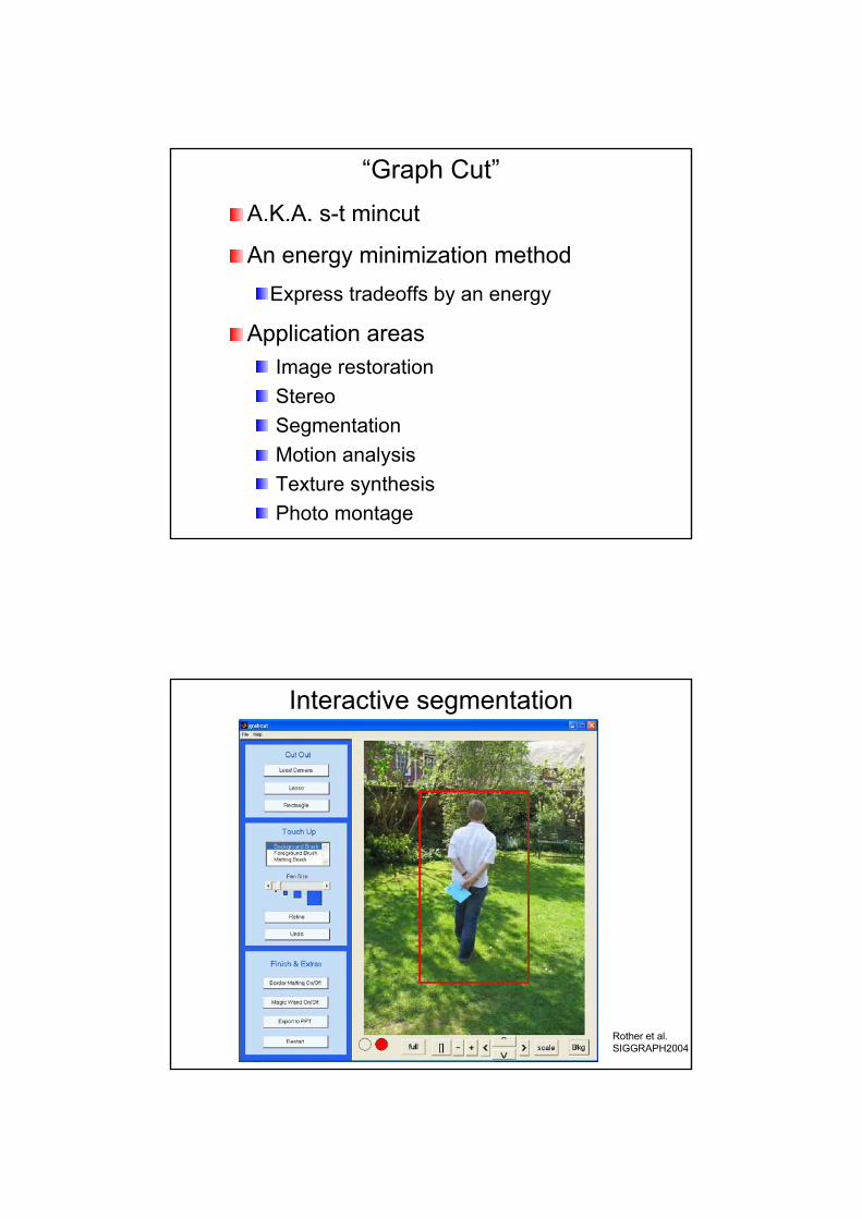
“Graph Cut”A.K.A. s-t mincut
An energy minimization methodExpress tradeoffs by an energy
Application areasImage restorationStereoSegmentationMotion analysisTexture synthesisPhoto montage
Interactive segmentation
Rother et al.SIGGRAPH2004

Boykov&JollyICCV2001
Interactive segmentation
Wang et al. SIGGRAPH2005
Interactive segmentation

Texture synthesis
Kwatra et al. SIGGRAPH2003
Kwatra et al. SIGGRAPH2003
Texture synthesis

Interactive photomontage
Agarwala et al. SIGGRAPH2004
StereoLeft Right Elevation map

History
Probablistic methods (SA, ICM,…) have been used for energy minimization
OR has used graph cut for ever
Was used for image processing in late 80’s
Introduced in vision in late 90’sSome theoretical results rediscovered(some were new)
Also used in graphics in recent years
Contents
Overview / Brief history
Energy minimization
Graphs and their minimum cuts
Energy minimization via graph cuts
Global minimization
Approximation methods
Energy design for graph cut

Example: Binary image restorationDenoising
Only the noisy image Y is given
On what basis do we know what is noise?We assume that the original image does not change too much between pixels (Smoothness assumption)
Close to the given image Y but not too rough
Express the Tradeoffs by an energy E( X )
XYClose to Y Doesn’t change
between pixels
∑∑∈∈
−+−=Evu
vuVv
vv XXXYXE),(
||||)( κλ
Find X that minimizes the energy
All pixels
Assigns Xv (= 0 or 1) to each pixel v
Example: Binary image restoration
XY
Neighboringpixels
Close to Y Doesn’t change between pixels

Find X that minimizes the energyExample: Binary image restoration
∑∑∈∈
−+−=Evu
vuVv
vv XXXYXE),(
||||)( κλ
隣接するピクセルの組
Neighboring pixels0 if Yv = Xvλ if Yv ≠ Xv
XY0 0 0 λ0 0 0 0λ 0 0 0
XY
All pixels
Assigns Xv (= 0 or 1) to each pixel v
Close to Y Doesn’t change between pixels
∑∑∈∈
−+−=Evu
vuVv
vv XXXYXE),(
||||)( κλ
ピクセル全部0 if neighbors arethe same; κ if not X
Find X that minimizes the energyExample: Binary image restoration
XY
Assigns Xv (= 0 or 1) to each pixel v
Neighboringpixels
Close to Y Doesn’t change between pixels
κκκ κκ

Energy minimization
In general, consider an energy of the form:
where V is a set of sitesE is a set of neighboring pairs of sitesX assigns a label to each site in V
First order Markov Random Field (MRF)
Problem: Find the X that minimizes E(X )
Data term Smoothing term
∑∑∈∈
+=Evu
vuuvVv
vv XXhXgXE),(
),()()(
Problem: Find the X that minimizes E(X )
The number of possible Xs is vast
Assignments of a label to each site in V
If V is 64×64 and labels are binary, 24096 (>101233) ways
The general problem is NP-Hard (Discovery of less-than-exponential-time algorithm unlikely)
Traditional method: Monte Carlo
In some cases, Graph Cut can minimize globally
Energy minimization

Contents
Overview / Brief history
Energy minimization
Graphs and their minimum cuts
Energy minimization via graph cuts
Global minimization
Approximation methods
Energy design for graph cut
Graphs and their minimum cuts
Directed graph
G = (V, E )
V :Finite set E ⊂ V ×V(Vertices) (Edges)
“Weight” on each edge
c: E→ R
u v(u,v)
u vc(u,v) =2
1 4
3

13
2
1
4
32
s
t
ST
Cost: 10
Graphs and their minimum cutsTake two vertices s, t of a weighted directed graph G
A cut of G w.r.t s and t is a partition of the vertices
into two groups (S,T ) such that
V = S ∪ T, S ∩ T = ∅
s∈S, t∈TTotal sum of the weightsof the edges going from
S to T is called the cost of (S,T )
Among the cuts of G with respect to s and t, ones with the smallest cost are called the minimum cuts
Mincut = MaxflowFord & Fulkerson Theorem (1956)Consider water flow from s to t, supposing the weight asthe capacity of pipes
Minimum cuts are given by the
saturated edges for maximum flows
Minimum cut
5 1
34
3 2
t
4
3
1
3
1
32
s

Among the cuts of G with respect to s and t, ones with the smallest cost are called the minimum cuts
Mincut = Maxflow
When the weights are all nonnegative, Maxflowcan be found in polynomial time
The number of possible cuts ~ 2number of vertices
Minimum cut
Contents
Overview / Brief history
Energy minimization
Graphs and their minimum cuts
Energy minimization via graph cuts
Global minimization
Approximation methods
Energy design for graph cut

||)()(),(
vuEvuVv
vv XXXgXE −+= ∑∑∈∈
κ
v)1(vg
)0(vgCut
s
tXv = 0
Xv = 1
Graph-cut minimization (binary)
||)()(),(
vuEvuVv
vv XXXgXE −+= ∑∑∈∈
κ
κ
Xv = 0
Xv = 1
Cut
s
t
Graph-cut minimization (binary)

Image plane graph
2D case
s
t

3D case
s
t
One to one correspondence between X and cut
Energy = Cut cost
Find minimum cut to minimize energy
The weights must be all nonnegative
s
t
s
t
X 0 1 1 0 1 1 1 0 0 1 1 X 1 1 1 0 0 0 0 0 1 0 0
Graph-cut minimization (binary)

The weights must be all nonnegative
can be arbitrary
∑∑∈∈
+=Evu
vuuvVv
vv XXhXgXE),(
),()()(
)(xgv
2)0( −=vg
5)1( −=vg
3
0
5+
s
t
s
t
Graph-cut minimization (binary)
The weights must be all nonnegative
can be arbitrary
must satisfySubmodularity condition
∑∑∈∈
+=Evu
vuuvVv
vv XXhXgXE),(
),()()(
),( yxhuv
)0,1()1,0()1,1()0,0( uvuvuvuv hhhh +≤+
Graph-cut minimization (binary)
)(xgv

The weights must be all nonnegative
∑∑∈∈
+=Evu
vuuvVv
vv XXhXgXE),(
),()()(
u v
)1,1()0,0()0,1()1,0(
uvuv
uvuv
hhhh−−
+)1,1()0,1( uvuv hh −
)0,0()0,1( uvuv hh −
u v0 00 1
)1,1()0,1( uvuv hh −
)1,1()0,0()0,1()1,0(
uvuv
uvuv
hhhh−−
+
1 0)1,1(
)0,0()0,1(2
uv
uvuv
hhh
−−
1 1 )0,0()0,1( uvuv hh −s
t
Graph-cut minimization (binary)
)0,1()1,0()1,1()0,0( uvuvuvuv hhhh +≤+
The weights must be all nonnegative
Add same value for all 4 cases
∑∑∈∈
+=Evu
vuuvVv
vv XXhXgXE),(
),()()(
s
t
v
)1,1()0,0()0,1()1,0(
uvuv
uvuv
hhhh−−
+u v0 00 1
1 0
1 1
)1,1()0,1( uvuv hh −
)0,0()0,1( uvuv hh −
u
)0,1()1,0()1,1()0,0( uvuvuvuv hhhh +≤+
Graph-cut minimization (binary)
)1,0(uvh
)0,1(uvh
)1,1(uvh
)0,0(uvh

The weights must be all nonnegative
can be arbitrary
must satisfySubmodularity condition
Long known in OR
∑∑∈∈
+=Evu
vuuvVv
vv XXhXgXE),(
),()()(
)(xgv
),( yxhuv
Graph-cut minimization (binary)
)0,1()1,0()1,1()0,0( uvuvuvuv hhhh +≤+
∑∑∈∈
+=Evu
vuuvVv
vv XXhXgXE),(
),()()(
When there are >2 labels
If labels have an order:Globally minimizeable is a convex
function of
},,,{ 10 klllL L=),( jiuv llh⇔
ji −
Graph-cut minimization (multi-value)

∑∑∈∈
+=Evu
vuuvVv
vv XXhXgXE),(
),()()(
Graph-cut minimization (multi-value)
i
3
2
1
0
s
t
gv(l0)
gv(l1)
gv(l2)
gv(l3)
||),( jillh jiuv −= κ
i
3
2
1
0
∑∑∈∈
+=Evu
vuuvVv
vv XXhXgXE),(
),()()(
s
t
Graph-cut minimization (multi-value)
uvh~)(~),( jihllh uvjiuv −= , :convex In general:
)1(~)(~2
)1(~
−−+
−−
+−
jih
jih
jih
uv
uv
uv

Contents
Overview / Brief history
Energy minimization
Graphs and their minimum cuts
Energy minimization via graph cuts
Global minimization
Approximation methods
Energy design for graph cut
The smoothing term must be convex
Approximation algorithms α -β swap / α expansion (Boykov, Veksler, Zabih)Guaranteed to get within thefactor 2c of global minima
The Potts model (discriminate only same or not): c =1
⎟⎟⎟
⎠
⎞
⎜⎜⎜
⎝
⎛=
≠
≠
∈ ),(min
),(maxmax
,vuuvXX
vuuvXX
Vvu XXh
XXhc
vu
vu
Graph-cut minimization (multi-value)
good good bad
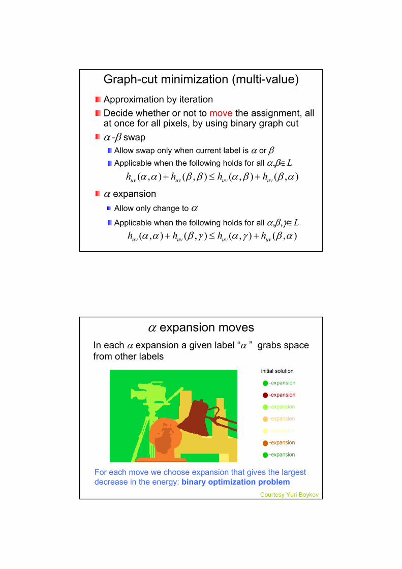
Approximation by iterationDecide whether or not to move the assignment, all at once for all pixels, by using binary graph cutα -β swap
Allow swap only when current label is α or βApplicable when the following holds for all α,β∈L
α expansionAllow only change to αApplicable when the following holds for all α,β,γ∈L
),(),(),(),( αββαββαα uvuvuvuv hhhh +≤+
),(),(),(),( αβγαγβαα uvuvuvuv hhhh +≤+
Graph-cut minimization (multi-value)
α expansion moves
initial solution
-expansion
-expansion
-expansion
-expansion
-expansion
-expansion
-expansion
In each α expansion a given label “α ” grabs space from other labels
For each move we choose expansion that gives the largest decrease in the energy: binary optimization problem
Courtesy Yuri Boykov

currentlabel
α
Optimal α expansion move
1D example
Courtesy Yuri Boykov
1. Start with any initial solution2. For each label α in any (e.g. random) order
1. Compute optimal α expansion move(s-t graph cuts)
2. Decline the move if there is no energy decrease
3. Stop when no expansion move would decrease energy
α expansion algorithm
Courtesy Yuri Boykov

α expansion algorithm vs. standard discrete energy minimization techniques
Single α expansion moveSingle “one-pixel” move(Simulated Annealing, ICM,…)
Large number of pixels can change their labels simultaneously
Finding an optimal move is computationally intensive
Only one pixel can change its label at a time
Finding an optimal move is computationally trivial
Courtesy Yuri Boykov
original image
α-expansion move vs.“standard” moves
a local minimumw.r.t. expansion moves
a local minimumw.r.t. “one-pixel” moves
noisy image
Potts energy minimization
Courtesy Yuri Boykov

Contents
Overview / Brief history
Energy minimization
Graphs and their minimum cuts
Energy minimization via graph cuts
Global minimization
Approximation methods
Energy design for graph cut
5 decisions for energy design
Example: DenoisingSites
PixelsNeighborhood structure
Pixel neighborhood structureLabels
Pixel colorsData term: How to reflect the given data
Make X closer to the given (noisy) imageSmoothing term:Desired propeties for X
Make neighboring pixels closer
∑∑∈∈
+=Evu
vuuvVv
vv XXhXgXE),(
),()()(
The space of X :Assignmnets of a label to each site

α -β swap α expansion
Boykov et al. PAMI 2001
ground truthSimulated Annealing
Disparity
Example 1: Stereo
SitesPixels of one of the images
Neighborhood structurePixel neighborhood structure
LabelsDisparities
Data termCompare pixels displaced according to the disparity
Smoothing termSmooth the disparities across neighborsBut also want to allow discontinuities at object boundariesMake smaller where intensity changes abruptly
∑∑∈∈
+ +−=Evu
vuuvVv
Xvv XXIIXEv
),(),Potts(||)( λ
⎩⎨⎧ =
= 1
)( 0),Potts(
mlml
)( ml ≠
RightLeft
uvλ
Example 1: Stereo

SitesPixels
Neighborhood structurePixel neighborhood structure
LabelsForeground or background (0 or 1)
Data termLocally assesses from the color of the pixel whether it is more like the foreground or the background
Smoothing termSmooth the labels across neighbors
∑∑∈∈
+=Evu
vuuvVv
vv XXhXgXE),(
),()()(Example 2: Segmentation
Data term: Creates histograms of the user-specified fore- and background sample pixelsEvaluates how likely to be fore- or background
is normalized
: FG histogram : BG
1,0 )),((log)( =−= llvIlgv θ
)0,(cθ
θ 1)1,()0,( ∑∑ ==cc
cc θθ
c
θ
c
θ
Example 2: Segmentation
)1,(cθ

Smoothing term: Potts (Penalty is smaller if the color changes more between neighbors)
Meant to cut where there is a strong contrast
⎪⎪⎩
⎪⎪⎨
⎧
′≠
′=
=′ −−
)(),dist(
)(0
),( 2)}()({
llvu
e
ll
llh vIuIuv κλ
Does not dependon labels
Example 2: Segmentation
Automatic
Userinteraction
segmentation
Rother et al.SIGGRAPH2004
Example 2: Segmentation
Automaticsegmentation

Agarwala et al. SIGGRAPH2004
Example 3: Photomontage
Example 3: Photomontage
Agarwala et al. SIGGRAPH2004

Sites/NeighborhoodPixel/Pixel neighborhood structure
LabelsWhich source picture (1, 2, ..., k)
Data termWhere a source picture is specified, a constant penalty for other labels
0 elsewhere
)'()'(0
)(llll
Mlgv ≠
=
⎩⎨⎧
=
Example 3: Photomontage
Smoothing termMakes boundary invisible (Reverse of segmentation)
Penalty is smaller if the color is closerOther cues (e.g. color gradient) could be matched
))(),(dist())(),(dist(),( vIvIuIuImlh mlmluv +=
Example 3: Photomontage

Rother et al. CVPR2005
Example 4: Digital Tapestry
Divide both tapestry and source into blocksSite: tapestry blocksNeighborhood: All pairs&block neighbors (later)Labels: Pairs of (source image, block shift)
Source 1
Source 2
shift −2
(1,−2) (1,−2) (2,1) (2,1)(1,−2) (1,−2) (2,1) (2,1)(1,−2) (1,−2) (2,1) (2,1)
Example 4: Digital Tapestry
shift 1

Data term: Block saliency (really the contrast)Central blocks are considered more salient than peripherals
Smoothing term:Each source block used once (All sites are neighbors)Neighboring block compatibility (Neighbor on tapestry)
(1,−2) (1,−2) (2,1) (2,1)(1,−2) (1,−2) (2,1) (2,1)(1,−2) (1,−2) (2,1) (2,1)
Source 1
Source 2
shift −2
Example 4: Digital Tapestry
shift 1
This has been an introduction, but...
Graph cut is an ongoing research area
Recent topics include
α -β range moves (Veksler CVPR2007)
Uses multi-label GC to minimize truncated convex potential
QPBO (Boros, Hammer, et al. RUTCOR Report RRR 10-2006; Kolmogorov&Rother CVPR2007)Minimizes even nonsubmodular energies where possible
Fusion moves (Lempitsky et al. ICCV2007)
Fuses current and proposed configurations à la α expansion
Higher-order energies (Ramalingam et al. CVPR2008)

ConclusionGraph cut: energy minimization
Energy form dictates applicable algorithmBinary (Submodular → global optimization)
Multi label (Global optimization in some cases)
Multi label (Approximation algorithms)
Some energy can be minimized globally
Approximations applicable to more general cases are often better than classical methods, e.g., SA
Code available at Kolmogorov's website:http://www.adastral.ucl.ac.uk/~vladkolm/software.html


