
Journal of Computational Physics 196 (2004) 126–144
www.elsevier.com/locate/jcp
A numerical method for three-dimensional gas–liquidflow computations
Yue Hao a,1, Andrea Prosperetti a,b,*
a Department of Mechanical Engineering, The Johns Hopkins University, 223 Latrobe Hall, 3400 N. Charles St.,
Baltimore, MD 21218, USAb Department of Applied Physics, Twente Institute of Mechanics, and Burgerscentrum, University of Twente,
AE 7500 Enschede, The Netherlands
Received 7 October 2002; received in revised form 14 October 2003; accepted 16 October 2003
Abstract
A numerical method for multiphase flow computations based on a finite-difference formulation with a fixed grid is
described. The method combines ideas from front tracking and the Ghost Fluid Method, with a numerical technique for
velocity extrapolation near the interface. It is shown that the method is able to solve three-dimensional free-surface flow
problems with an incompressible liquid and a compressible gas maintaining the interface sharp. Numerical results are
compared with numerical solutions of the Rayleigh–Plesset equation for the free oscillation of a gas bubble, and in-
dependent front-tracking results for buoyant bubbles. Finally, the effects of an imposed sinusoidal liquid flow on a gas
bubble are investigated.
� 2003 Elsevier Inc. All rights reserved.
AMS: 65M06; 76T10
Keywords: Numerical method; Two-phase flow; Bubble; Front tracking; Computational fluid dynamics
1. Introduction
Particularly for three-dimensional problems, multiphase flow computations are notoriously difficult due
to the presence of a deformable phase boundary. For this reason, such computations have attracted
considerable attention, and a variety of numerical techniques has been developed in the last decade.Even though some success has been achieved by the use of boundary fitted grids [30] and Lagrangian
methods with moving grids [9,12,16,27,31], fixed grid methods associated with interface capturing
*Corresponding author. Tel.: +1-410-516-8534; fax: +1-410-516-7254.
E-mail address: [email protected] (A. Prosperetti).1 Present address: Lawrence Livermore National Laboratory, Livermore, CA 94550, USA.
0021-9991/$ - see front matter � 2003 Elsevier Inc. All rights reserved.
doi:10.1016/j.jcp.2003.10.032

Y. Hao, A. Prosperetti / Journal of Computational Physics 196 (2004) 126–144 127
algorithms such as the volume of fluid (VOF) [2], level-set [3,8,28,29], and front tracking [32–34] are
popular because of their comparatively simple implementation and easy extension to three dimensions.
In comparison with interface-capturing methods, in which the interface evolution is ‘‘captured’’ indi-rectly through the volume-fraction distribution (VOF) or the zero-level-set of the distance function, front-
tracking methods, in which the front is explicitly tracked by marker points, possess an advantage in that the
explicit knowledge of the interface reduces by a considerable amount the resolution needed to maintain
accuracy. Moreover, explicit front tracking permits more than one interface in a single computational cell
without coalescence, which can find important applications in dense bubbly flows, emulsions, etc.
The finite-difference/front-tracking method developed by Tryggvason and co-workers has achieved re-
markable success in two- and three-dimensional multiphase flow simulations [32–34]. The core of the
method is the ‘‘one-field formulation’’ of the Navier–Stokes equations in which both phases are consideredincompressible [25,34]: a single set of conservation equations is established in the whole field containing two
different immiscible fluids, and the material property jumps like density, viscosity, etc. across the interface
are discretized smoothly by the ‘‘immersed boundary’’ method [20,21] and so are the surface tension and
other interfacial terms.
In the ‘‘immersed boundary’’ method, a smeared d-function approximation is applied to force continuity
of the numerical solution within a thin artificial layer around the interface, in spite of the fact that the
physical solution possesses a jump at the interface. This procedure leads to a numerical smearing of the
interface. In many simulations of isothermal multiphase flows, this artificial layer can be kept thinner thanthe physical boundary layer, and therefore it does not compromise the solution accuracy. However, under
some circumstances – for example when phase change occurs at the surface of a vapor bubble – an adverse
effect of the numerical smearing may be seen in the heat transfer calculation since the thermal penetration
depth into the liquid becomes so small [15] as to be comparable to the ‘‘artificial’’ layer. Moreover, the
‘‘one-field formulation’’ will not be applicable in some other two-phase flow problems such as acoustic
cavitation, in which compressible gas bubbles are embedded in a (nearly) incompressible liquid.
Motivated by the above-mentioned difficulties, a series of recent publications (see e.g. [3,5–8,18,19]) has
returned to an older boundary-capturing approach [14] (see also [13]), now known as the Ghost FluidMethod (GFM). This work and its relevant extensions have drawn considerable attention in recent years.
The basic idea (implemented together with a level-set method), is to extrapolate the ‘‘real’’ solution values
in each phase onto fictitious ghost nodes located in the other phase, and then solve the governing equations
in both phases separately. The important feature of this method lies in the fact that the property discon-
tinuities and jump conditions at the interface are well preserved.
In this paper, we consider two-phase flow problems with an incompressible liquid and a compressible gas
and propose a new numerical method obtained as a hybrid of three-dimensional front-tracking [32,34],
Ghost Fluid Method (GFM) [8,18,19], and a numerical technique for velocity extrapolation near the in-terface [23]. Although the original motivation for the development of this new method was the need to
maintain a sharp interface with an eye toward applications to heat-transfer problems, here we limit our-
selves to isothermal systems in order to describe the approach in a simple context and to be able to compare
the results with those given by other existing methods.
2. Governing equations
The fluid motion in the liquid is assumed to be incompressible and governed by the Navier–Stokes
equations, which can be expressed in conservative form as:
oðquÞot
þr � ðquuÞ ¼ �rp þ qgþr � s; ð1Þ
128 Y. Hao, A. Prosperetti / Journal of Computational Physics 196 (2004) 126–144
r � u ¼ 0: ð2Þ
Here t, q , u, p and g represent time, liquid density, velocity, pressure, and body force, and s is the viscousstress tensor,
s ¼ l ruh
þ ruð ÞTi; ð3Þ
in which l denotes liquid viscosity and the superscript T the transpose.
The examples used later to illustrate the performance of the method involve dynamic processes of gas
bubbles in a liquid, even though the numerical technique presented here can also be extended to other two-
phase flow phenomena. Since, with these examples, we focus on the manner in which the interface is
handled in the presence of volume changes of the gas region, we will adopt a common simplification to
calculate the gas pressure in the gas region: the gas pressure pg is assumed spatially uniform inside the
bubble and related to the instantaneous bubble volume V by a polytropic law of compression (see e.g. [22]),
pg ¼ p0V0V
� �c
; ð4Þ
where c is the polytropic index, and V0 and p0 are the equilibrium volume of the bubble and the corre-
sponding pressure, respectively. In the case of several bubbles modeled in a similar manner, each bubble
would have its own values of V0, p0, and possibly c. If the present method were coupled with a calculation of
the energy equation, one might use, e.g., the liquid–vapor saturation relation to establish the bubble in-
ternal pressure. At another level of complexity, the compressible Navier–Stokes equations could be solvedin the gas region by extending the ideas that we describe below.
The pressure on the liquid side of the interface CðtÞ is related to the bubble internal pressure by the
balance of normal stresses across the interface, namely,
p ¼ pg � rjþ n � s � nð Þ; ð5Þ
where n is the unit normal to the interface drawn outwards from the bubble, r is the surface tension co-
efficient, and j the curvature of the interface which can be computed from
j ¼ r � n: ð6Þ
Moreover, the zero tangential stress boundary condition,
n� ðs � nÞ ¼ 0; ð7Þ
is imposed on the interface [23].
3. Numerical method
Our method is based on a finite difference formulation on a fixed grid and a front-tracking approach. It
consists of several elements, which are now described in turn and finally combined into the algorithm.
3.1. Interface-tracking approach
The interface-tracking method is applied to capture the position and shape of the interface whose motion
is followed [32–34]; in other words, the evolution of the interface separating the two phases is explicitly
tracked by an unstructured moving grid of lower dimension.

Y. Hao, A. Prosperetti / Journal of Computational Physics 196 (2004) 126–144 129
3.1.1. Front construction
In three-dimensional two-phase flow computations, the two-dimensional interface is constructed by
Lagrangian marker points which are connected by triangular elements. The points and elements areproperly labeled and oriented in such a way that the calculated normal direction for each element is drawn
from the gas into the liquid domain. Since more details illustrating the front structure can be found in [32–
34], we do not elaborate here. Fig. 1 shows examples of unstructured coarse and fine grids on the surface of
a spherical bubble.
3.1.2. Indicator function
Since we treat the liquid and gas regions in different ways, it is required that we be able to distinguish
them properly and, particularly near the explicitly marked interface, to identify the fixed grid nodes whichfall within the liquid domain on which the finite difference discretization of the Navier–Stokes equations (1)
and (2) with appropriate boundary conditions (5) and (7) is carried out. For this and other purposes to be
discussed in a later section, we adopt the idea of an indicator function, which was originally introduced and
used for evaluating ‘‘one-field’’ material properties in Tryggvason�s front tracking implementation [32–34].
The indicator function Iðx; tÞ, which is based on a Heaviside function and designed to be 1 if at time tgrid position x is in the liquid and �1 in the gas, is constructed from the known position of the interface
from
Iðx; tÞ ¼ 1� 2
ZVg
d3y dð3Þðx� yÞ; ð8Þ
where the integral is over the region Vg occupied by the gas and dð3ÞðxÞ is a three-dimensional d-distributionobtained as the outer product of one-dimensional ones, dð3ÞðxÞ ¼ dðxÞdðyÞdðzÞ. Upon calculating the gra-
dient we find
rIðx; tÞ ¼ �2
ZVg
d3yrdð3Þðx� yÞ ¼ 2
ZVg
d3yrydð3Þðx� yÞ ¼ 2
ICðtÞ
dSy ndð3Þðx� yÞ; ð9Þ
where the last integral is over the interface CðtÞ. The first step in (9) follows from the dependence of the d-function on the difference ðx� yÞ and the last step is a consequence of the (generalized) divergence theorem.
Upon taking the divergence of (9) we have the following Poisson equation for the indicator function,
Fig. 1. Two examples of interface grids on a bubble. Left: coarse grid; right: fine grid.

130 Y. Hao, A. Prosperetti / Journal of Computational Physics 196 (2004) 126–144
r2I ¼ r � 2
ICðtÞ
dSy ndð3Þðx
� yÞ
!: ð10Þ
Note that the Poisson equation on a regular domain can be solved by traditional fast Poisson solvers and
the right-hand side of the equation, a function only of the known interface position, is numerically treated
by replacing the d-distribution by a smooth approximation which leads to a discrete approximation of the
integral:ZCðtÞ
dSy ndð3Þðx� yÞ ¼
Xl
DlijknlDSl: ð11Þ
DSl and nl are the area of, and unit normal to, element l, and Dlijk is a regularized delta distribution, given
near the point x � ðxi; yj; zkÞ, by [32]
Dlijkðyp � xÞ ¼ dðxp � ihÞdðyp � jhÞdðzp � khÞ; ð12Þ
in which yp ¼ ðxp; yp; zpÞ denotes the geometric center of the surface element l, h the grid spacing, and dðrÞ istaken as [20]
dðrÞ ¼ ð1=2nhÞ½1þ cosðpr=nhÞ�; jrj < nh;0; jrjP nh:
�ð13Þ
As a consequence of this regularization, the numerical solution of the Poisson equation (10) gives a con-
tinuous indicator function Iðx; tÞ increasing smoothly from )1 in the gas to 1 in the liquid over a distance of
the order nh from the actual interface. In this step, we usually take the parameter n as 4. The use of this
relatively large value of n increases the smoothing of the front. Since we assign each node to the liquid or
gas region according to the sign of I , this smoothing permits an accurate localization of the grid nodes intheir appropriate phase. Furthermore, the accuracy of the calculation of the normal, found from a finite
difference approximation to rI=jrI j, is also improved. It should be stressed that, unlike the level-set
method, here the indicator function is not used to capture the location of the interface, which is always
explicitly identified by the marker points, but only to decide which phase the grid points belong to. In
particular, the difficulty with mass (or volume) conservation which sometime affects level-set calculations is
avoided.
3.1.3. Front advancement
The interface is advanced in a Lagrangian fashion by integrating
dy
dt¼ vðy; tÞ; ð14Þ
with v standing for the interfacial velocity. In the absence of phase change, we may simply write the fluid
velocity at the interface as
vðy; tÞ ¼ZV ðtÞ
d3xdð3Þðy� xÞuðx; tÞ; ð15Þ
where the integral is over a volume surrounding the interfacial point y. As before, the d-function can be
approximated by the smooth distribution (12) and (13) so that
vLðy; tÞ ¼Xijk
DijkðyÞuLðxi; yj; zk; tÞDVijk; ð16Þ

Y. Hao, A. Prosperetti / Journal of Computational Physics 196 (2004) 126–144 131
with the summation extended to the ði; j; kÞ grid points near the interface point y under consideration and
the subscript L denoting the Lth velocity component. In calculating the Dijk used in the front velocity in-
terpolation, we take n in (13) to be 2 as suggested by Peskin [20].
3.2. Finite difference formulation
The front advancement from time level n to nþ 1 is treated explicitly by discretizing the relation (14) as
ynþ1p ¼ ynp þ vnpDt; ð17Þ
where the subscript p identifies the generic point on the front with position yp and velocity vnp; this velocity is
interpolated from the grid values close to the front according to (16).
With the assumption that both q and l are constant in the incompressible liquid, the first-order pro-
jection method [4] is applied and Eq. (1) is discretized on a MAC grid as
u� � un
Dt¼ �rh � ðununÞ þ
lrh � rhun þ rhu
nð ÞTh i
qþ g ð18Þ
and
unþ1 � u�
Dtþrhp
q¼ 0; ð19Þ
where the subscript h indicates the standard central-difference discretization of the gradient. Once the in-
termediate velocity u� is computed, a correction step is taken such that the velocity at the new time levelnþ 1 is divergence-free (2),
rh � unþ1 ¼ 0; ð20Þ
which causes the elimination of unþ1 from Eq. (19), resulting in
r2hp ¼ q
Dtrh � u�; ð21Þ
coupled with the pressure jump (5) at the interface and the known gas pressure predicted by (4) at the nþ 1
time level. The technique of solving the pressure equation will be discussed in Section 3.4. After the pressure
is obtained, the velocity unþ1 can be updated from
unþ1 ¼ u� � Dtqrhp; ð22Þ
which completes the time step.
3.3. Velocity extrapolation
From the above finite difference scheme, it is obvious that even though the Navier–Stokes equations are
only solved on the fixed grid within the liquid domain, if we want to avoid the use of irregular stencils, we
need to extrapolate the liquid velocity field far enough into the gas in order not only to resolve the ad-
vection and viscous terms (18) on the nodes adjacent to the interface on the liquid side, but also for ad-vecting the marker points of the front (17). The velocity extrapolation may be carried out in various ways
[5,6,23]. Here, we apply a Lagrange multiplier method in which the zero tangential stress boundary con-
dition on the interface (7) is taken as the constraint; this approach is due to Popinet and Zaleski [23] who

132 Y. Hao, A. Prosperetti / Journal of Computational Physics 196 (2004) 126–144
developed it for an axisymmetric problem. We extend their technique to the general three-dimensional case
as follows.
In order to extrapolate the liquid velocity to a point P in the gas near the interface (Fig. 2), we assumethat the local velocity field around P can be expressed as
u ¼ u0 þ T � x; ð23Þ
where u0 ¼ ðu0; v0;w0Þ is a constant, x is the position vector and Tij ¼ oui=oxj is a constant 3� 3 matrix.
With this assumption the viscous stress s around point P can be approximated as l Tþ TT� �
.
If N grid points in the liquid domain are chosen in the neighborhood of the point P and the unit normal
np to the interface at P as well, then u0 and T can be computed by minimizing the error
U ¼XNn¼1
kðu0 þ T � xn � unÞk2 þ k � np�
� l T��
þ TT�� np��; ð24Þ
where k � k denotes the vector norm, xn and un represent the position vector and the corresponding velocity
of the grid nodes in the liquid, and the components ki (i ¼ 1; 2; 3) of k are Lagrange multipliers [17]. The
error U (24) is minimized by taking
oUoC
¼ 0; ð25Þ
where
C � u0; v0;w0; T11; T12; T13; T21; T22; T23; T31; T32; T33; k1; k2; k3ð Þ: ð26Þ
The resulting linear algebraic equations are solved by the Singular Value Decomposition method [24].
The N points are chosen in the liquid as shown in Fig. 2 (also in Fig. 4 of [23]) such that the cost
function,
XNn¼1
Dis2ðxn; LÞ2h
þ vdis2ðxn; xP Þi
ð27Þ
Fig. 2. Sketch to illustrate the explanation of the velocity extrapolation procedure around the generic point P .

Y. Hao, A. Prosperetti / Journal of Computational Physics 196 (2004) 126–144 133
has the minimum value. Here Disðxn; LÞ is the distance of the point xn from the line L coinciding with the nPdirection and passing through P , disðxn; xP Þ is the Euclidean distance between points xn and xP , and v a
geometrical parameter typically set to 1=2 [23]. Note that nP can be accurately approximated by taking thegradient of the indicator function, as mentioned before:
nP ¼ rIðxP ; tÞkrIðxP ; tÞk
: ð28Þ
In this use for this purpose, the indicator function plays a role analogous to the level-set function in the
level-set method [18,28].
3.4. Solving the pressure equation
After the unprojected velocity u� is obtained, solving the Poisson equation (21) in the liquid domain withthe pressure jump (5) applied at the interface is the next challenge in this problem.
As discussed in Section 1, there are two notable techniques to handle property jumps at the interface, the
‘‘immersed boundary’’ method [20] and the Ghost Fluid Method (GFM) and its extensions [5,6,13,14,19].
Due to the nature of the problem we consider here, we adopt a GFM-similar boundary condition
capturing approach [19] to treat the pressure jump at the interface C separating the liquid (incompressible)
and gas (compressible) domains.
From the point of view of a finite difference approximation, the pressure gradient across C in (21) is not
well behaved because of the jump conditions. For example, take the grid point ði; j; kÞ adjacent to C. If thePoisson equation (21) at ði; j; kÞ in the liquid domain is discretized in a standard finite difference fashion, we
find
1
Dxpiþ1;j;k � pi;j;k
Dx
� h� pi;j;k � pi�1;j;k
Dx
� iþ 1
Dypi;jþ1;k � pi;j;k
Dy
� �� pi;j;k � pi;j�1;k
Dy
� ��
þ 1
Dzpi;j;kþ1 � pi;j;k
Dz
� h� pi;j;k � pi;j;k�1
Dz
� i¼ q
Dt
u�iþ1=2;j;k � u�i�1=2;j;k
Dx
�þv�i;jþ1=2;k � v�i;j�1=2;k
Dyþw�
i;j;kþ1=2 � w�i;j;k�1=2
Dz
�; ð29Þ
with u, v, w are the x-, y- and z-velocity components. If any neighboring grid node, say ðiþ 1; j; kÞ, happensto reside in the gas phase and p�iþ1;j;k is taken as the gas pressure pg (4), then the corresponding pressure
gradient term across C,
p�iþ1;j;k � pþi;j;kDx
; ð30Þ
will not be well-behaved. In order to avoid this difficulty, we must exclude the effect of the pressure jump (5)
with its discrete version as
p�iþ1;j;k � pþi;j;k ¼ J iþ1C ¼ rj½ � ðn � s � nÞ�C; ð31Þ
in which J iþ1C is the pressure jump at C between grid points ðiþ 1; j; kÞ and ði; j; kÞ.
It is legitimate to use a ghost value pþiþ1;j;k in the gas in defining the pressure gradient instead of the real
one p�iþ1;j;k ¼ pg, provided these two are related by the pressure jump J iþ1C ,
pþiþ1;j;k ¼ p�iþ1;j;k � J iþ1C ; ð32Þ

134 Y. Hao, A. Prosperetti / Journal of Computational Physics 196 (2004) 126–144
which leads to a reasonable definition of the pressure gradient,
pþiþ1;j;k � pþi;j;kDx
¼p�iþ1;j;k � pþi;j;k
Dx� J iþ1
C
Dx: ð33Þ
Then Eq. (33) is substituted into (29) and the extra generated term J iþ1C =Dx is moved to the right-hand side.
It should be noted that we can find Ji;j;k at each grid node (i; j; k) near the interface, provided that n at point
ði; j; kÞ is calculated by taking the gradient of the indicator function (28) and so are the curvature j (6) andthe normal viscous stress term n � s � n. The normal viscous stress term at grid nodes located in the gas is
obtained from the extrapolated velocity field found before. With the aid of the indicator function I , the J iþ1C
at C is interpolated by
J iþ1C ¼ Jiþ1;j;kjIi;j;kj þ Ji;j;kjIiþ1;j;kj
jIi;j;kj þ jIiþ1;j;kj: ð34Þ
All derivatives involving the jump condition, if any, in (29) can be treated in the same way. After the
above-mentioned treatment, the Eq. (29) is arranged as
1
Dxpiþ1;j;k � pi;j;k
Dx
� h� pi;j;k � pi�1;j;k
Dx
� iþ 1
Dypi;jþ1;k � pi;j;k
Dy
� �� pi;j;k � pi;j�1;k
Dy
� ��
þ 1
Dzpi;j;kþ1 � pi;j;k
Dz
� h� pi;j;k � pi;j;k�1
Dz
� i¼ q
Dt
u�iþ1=2;j;k � u�i�1=2;j;k
Dx
�þv�i;jþ1=2;k � v�i;j�1=2;k
Dyþw�
i;j;kþ1=2 � w�i;j;k�1=2
Dz
�þ J iþ1
C
Dxð Þ2þ J i�1
C
Dxð Þ2
þ J jþ1C
Dyð Þ2þ J j�1
C
Dyð Þ2þ Jkþ1
C
Dzð Þ2þ Jk�1
C
Dzð Þ2: ð35Þ
It can be seen that with Dirichlet (or Neumann) boundary conditions the above equations in the liquid
phase coupled with the known values p�i;j;k(pg) calculated from (4) in the gas constitute a symmetric linear
system, which is solved by a stabilized conjugate gradient squared (CGSTAB) method [11,35].
It may be noted that, with this procedure, the matrix of the linear system for the pressure is symmetric
and independent of the density contrast between the phases. Thus, the convergence difficulties which
sometimes prevent the use of realistic density values with the original front-tracking method are obviated.This is a particularly useful feature for phase-change calculations, where the actual vapor density must be
kept at its physical value to avoid errors in the latent heat calculation.
3.5. Numerical algorithm
The steps of the numerical procedure described above may be summarized as follows:
1. The computational step begins with an explicit advancement of the front (14) to the new position by the
interpolated interface velocity (16).2. With this new position of the front at time level nþ 1, update the indicator function Iðx; tÞ by solving
the Poisson equation (10).
3. Identify the velocity and pressure nodes located in the gas and liquid regions from the sign of the indi-
cator function.
4. Update the pressure pnþ1g in the gas domain from (4), after computing the gas volume.
5. Extrapolate the velocity field in the liquid far enough into the gas region as outlined in Section 3.3.
6. Compute the intermediate value of the new velocity field u�.

1
F
a
3
Y. Hao, A. Prosperetti / Journal of Computational Physics 196 (2004) 126–144 135
7. Project u� onto its divergence-free component in the region identified by Iðx; tÞP 0 and solve for the
pressure pnþ1 from the Poisson equation (35) taking into account the pressure jump (5) at the interface.
Note that the surface tension and viscous normal stress are calculated on the nearby grid points, and
thereafter interpolated on the front.8. Update the velocity field unþ1 from the new pressure pnþ1 (22).
9. Repeat step 5 with the updated velocity field unþ1 in the incompressible region so that all velocities near
the interface are consistently available at time level nþ 1.
0. Move to the next time level.
4. Validation tests
We now compare the results of the present method with those obtained by independent methods to
demonstrate its accuracy. All these other results are obtained from models or codes which have been amply
verified against experiment. Thus, agreement with them also ensures that our results would agree with
experiment, and we do not need to carry out an experimental validation explicitly. The first example shows
how the calculation of a compressible gas region can successfully be coupled with that of an incompressible
liquid. In the remaining examples, the gas region is effectively incompressible, so as to be able to compare
our results with those of the original front-tracking method.
4.1. A spherical bubble in an unbounded liquid
In this test, we compare the numerical solution for the free oscillations of a gas bubble as given by our
method with that given by the Rayleigh–Plesset equation [22], which describes the radial motion of a
spherical bubble in an unbounded fluid,
R€Rþ 3
2_R2 ¼ 1
qpg
� p1 � 2r
R� 4l
_RR
!; ð36Þ
where p1 represents the ambient pressure and R the instantaneous bubble radius.
ig. 3. Comparison between the present Navier–Stokes solution and the Rayleigh–Plesset solution [22] for the free radial oscillation of
stationary gas bubble with an equilibrium diameter of 47.5 lm released from an initial diameter of Di ¼ 50 lm. The grid resolution is
60� 360� 360 on a domain of 12Di � 12Di � 12Di.

136 Y. Hao, A. Prosperetti / Journal of Computational Physics 196 (2004) 126–144
In the test case shown below, since we consider a stationary, initially over-expanded gas bubble in an
unbounded liquid, free inflow/outflow boundary conditions are applied on all the boundaries of the
computational domain. The equilibrium radius R0 is 23.75 lm and the bubble is released at time 0 from aslightly over-expanded state, Rð0Þ ¼ 25 lm, so that it executes damped free oscillations. The other physical
parameters have values appropriate for water: liquid density q ¼ 1000 kg/m3, surface tension r ¼ 0:07 N/m,
viscosity l ¼ 0:001 kg/m s, c ¼ 1.4, p1 ¼ 1 atm.
We found that, in order to reduce the boundary effects, it was very important to use a large compu-
tational domain with a reasonably high resolution. We used a domain size equal to 12 times the bubble
initial diameter and 360� 360� 360 nodes to ensure that the maxima and minima of the oscillation were
adequately resolved.
The present results (open squares) are compared with the Rayleigh–Plesset ones (solid line) in Fig. 3. It isseen that there is a very good agreement between the two. We did not attempt a similar comparison for a
larger initial over-expansion for reasons of computational time, and also because the spherical shape of
oscillating bubbles is known to become unstable at high amplitude. This physical instability of course
Fig. 4. Comparison between the present numerical simulations and those by Tryggvason�s finite difference/front-tracking (FD/DT)
method [34] for a buoyant bubble with Eo ¼ 3:57 and Mo ¼ 3� 10�7. The nondimensional initial bubble radius Ri is 0.25. The
60� 60� 120 grids are on a 1� 1� 2 domain. The snapshot pairs shown are taken at times 0.10, 0.15, 0.20, 0.25, 0.30, 0.35, 0.40, 0.45,
and 0.5 (left to right, top to bottom).

Y. Hao, A. Prosperetti / Journal of Computational Physics 196 (2004) 126–144 137
would be entirely missed by the Rayleigh–Plesset solution, which would prevent a meaningful comparison
with our results.
4.2. Comparison with the finite difference/front-tracking method
In the previous test, the bubble was stationary and spherical. Now we compare our numerical results
with those obtained from Tryggvason�s finite difference/front-tracking method [34] for the case of a bubble
rising under gravity. Compressibility effects inside the gas bubble can be ignored when the bubble rises over
a sufficiently short distance. Thus, it is legitimate to make a comparison between the two approaches for
buoyant bubble simulations, even though in Tryggvason�s front-tracking method the gas is assumed to be
incompressible.Two nondimensional numbers, the E€otv€os number (Eo ¼ qgD2
i =r) and the Morton number
(Mo ¼ gl4=qr3), are used to describe the process, in which Di is the initial bubble diameter.
Fig. 4 shows a series of snapshots taken at different times during the bubble rise. For this case, Eo ¼ 3:57andMo ¼ 3� 10�7. For a liquid with viscosity l ¼ 0:01 kg/m s and other properties equal to those of water,
at normal gravity, these values are for an air bubble with Di ¼ 5 mm. In each snapshot, both our results and
those for Tryggvason�s finite difference/front-tracking (FD/FT) method are presented. As the bubble rises,
it becomes ellipsoidal. In order to quantify the comparison, we ‘‘measure’’ the bubble shape in terms of the
bubble ‘‘horizontal’’ and ‘‘vertical’’ diameters during the bubble motion. The comparison between the twosets of results is shown in Fig. 5. It can be seen that the comparison is quite good but shows indications of
diverging from the FD/FT results around the end of the simulation at t ¼ 0:5. We believe that this dif-
ference can be eliminated by using more nodes, but have not done so for lack of adequate computational
resources.
In the test which follows (Figs. 6 and 7), we decrease the surface tension by one order of magnitude, and
thus have larger E€otv€os (Eo ¼ 35:7) and Morton numbers (Mo ¼ 3� 10�4). As a result, the pressure force
exerted along its surface transforms the bubble into a spherical-cap-like shape. In Fig. 6, we have a
horizontal view of the rising bubble while Fig. 7 shows pictures taken looking from below. Fig. 8 is similarto Fig. 5 and compares the bubble horizontal and vertical diameters as calculated by the two methods.
Fig. 5. Comparison between the horizontal and vertical bubble dimensions as computed by the present method and Tryggvason�sfinite-difference/front-tracking (FD/DT) method [34] for the buoyant bubble of the previous figure.

Fig. 6. Comparison between the present numerical simulations and Tryggvason�s finite difference/front-tracking (FD/DT) results [34]
for a buoyant bubble with Eo ¼ 35:7 and Mo ¼ 3� 10�4. The nondimensional initial bubble radius Ri is 0.25. The 60� 60� 120 grid
covers a 1� 1� 2 domain. The snapshots are taken in the horizontal direction and are at times 0.10, 0.15, 0.20, 0.25, 0.3, and 0.35 (left
to right, top to bottom).
138 Y. Hao, A. Prosperetti / Journal of Computational Physics 196 (2004) 126–144
Again, it is seen that there is generally a good agreement between our results and those for the finite dif-
ference/front-tracking (FD/FT) method.
Fig. 9 shows the velocity distribution around the buoyant bubble as computed with the present
method. A cut is made through the center of the bubble for a clearer look at the velocity field in its
vicinity.
5. A gas bubble in a sinusoidal flow
In this section, we present an example of the application of this numerical method to a case in which the
compressibility of the gas in the bubble is important. This situation cannot be treated by the original front-
tracking method.

Fig. 7. Comparison between the present numerical simulations and Tryggvason�s finite difference/front-tracking (FD/DT) method
results [34] for a buoyant bubble with Eo ¼ 35:7 and Mo ¼ 3� 10�4. The nondimensional initial bubble radius Ri is 0.25. The
60� 60� 120 grid covers a 1� 1� 2 domain. The snapshots are taken looking up toward the computational domain at the same times
as in the previous figure (left to right, top to bottom).
Y. Hao, A. Prosperetti / Journal of Computational Physics 196 (2004) 126–144 139
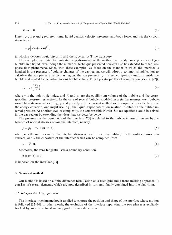
As sketched in Fig. 10, a gas bubble is set in a square tube and a sinusoidal inflow is imposed at the
bottom of the computational domain. At the exit of the domain outflow boundary conditions prevail while
no-slip boundary conditions are employed at the tube surface. Buoyancy is disregarded. The imposed in-flow velocity is
Vin ¼ Vmax½cosðx3tÞ þ sinðx2tÞ�; ð37Þ
where xn is the natural frequency of the nth mode of the bubble shape oscillation:
x2n ¼ ðn� 1Þðnþ 1Þðnþ 2Þ r
qR3e
: ð38Þ
with Re the equilibrium bubble radius. When the bubble is driven at the natural frequencies of shape os-
cillations (38) in this way, the surface modes n ¼ 2 and n ¼ 3 are both excited parametrically, which leads to
asymmetrical bubble shape oscillations. Consequently, the bubble propels itself. The relevant theoretical

Fig. 8. Comparison between the horizontal and vertical bubble dimensions as computed by the present method and Tryggvason�sfinite-difference/front-tracking (FD/DT) method [34] for the buoyant bubble of the previous two figures.
Fig. 9. Velocity profile around the buoyant bubble of the previous three figures as computed from our numerical simulation.
140 Y. Hao, A. Prosperetti / Journal of Computational Physics 196 (2004) 126–144
analysis and experimental observations for the self-propulsion of asymmetrically pulsating bubbles are
presented by Benjamin and Ellis [1], Feng and Leal [10], and Reddy and Szeri [26], and others. In the case
illustrated here, the size of the rectangular cell is 1 cm � 1 cm � 2 cm. An air bubble with radius of 0.25 cm
is located 0.5 cm away from the inlet of the cell. The inflow velocity amplitude is Vmax ¼ �1 mm/s. The other
physical parameters are the same as those used in Fig. 3. Under the action of the imposed sinusoidal inflow
(37), the bubble ‘‘swims’’, which is shown in Fig. 11 by plotting the bubble centroid position versus time. In
addition to translation, the compressibility of the gas makes the bubble volume oscillate as well. Figs. 12
and 13 present a sequence of snapshots during the bubble oscillation and translation.
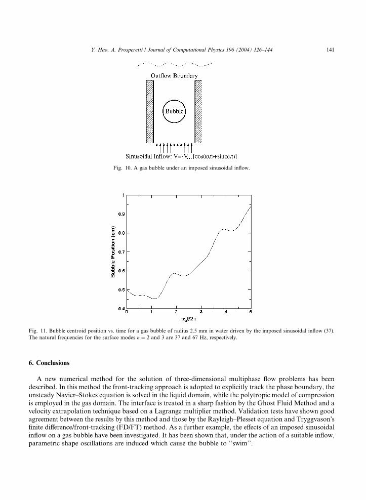
Fig. 11. Bubble centroid position vs. time for a gas bubble of radius 2.5 mm in water driven by the imposed sinusoidal inflow (37).
The natural frequencies for the surface modes n ¼ 2 and 3 are 37 and 67 Hz, respectively.
Fig. 10. A gas bubble under an imposed sinusoidal inflow.
Y. Hao, A. Prosperetti / Journal of Computational Physics 196 (2004) 126–144 141
6. Conclusions
A new numerical method for the solution of three-dimensional multiphase flow problems has been
described. In this method the front-tracking approach is adopted to explicitly track the phase boundary, the
unsteady Navier–Stokes equation is solved in the liquid domain, while the polytropic model of compression
is employed in the gas domain. The interface is treated in a sharp fashion by the Ghost Fluid Method and a
velocity extrapolation technique based on a Lagrange multiplier method. Validation tests have shown goodagreement between the results by this method and those by the Rayleigh–Plesset equation and Tryggvason�sfinite difference/front-tracking (FD/FT) method. As a further example, the effects of an imposed sinusoidal
inflow on a gas bubble have been investigated. It has been shown that, under the action of a suitable inflow,
parametric shape oscillations are induced which cause the bubble to ‘‘swim’’.

Fig. 12. Sequence of snapshots of the oscillating and translating bubble of the previous figure taken at dimensionless times (left to
right, top to bottom) x3t=ð2pÞ ¼ 0, 0.2060, 0.4001, 0.6051, 0.8100, 1.004, 1.209, 1.306, 1.403, 1.508, 1.603, 1.700, 1.808, 1.906, 2.007,
2.106, 2.206, and 2.305.
142 Y. Hao, A. Prosperetti / Journal of Computational Physics 196 (2004) 126–144
A prominent feature of this method is that it not only possesses the advantages of the explicit front-
tracking approach, but also treats the interface in a sharp fashion in contrast to the original front-tracking
method [34]. Further applications of the method may be found in many other multiphase flow problemssuch as bubbly flow, slug flow, turbulent multiphase flow and so on.
Efficiency is an important issue in multiphase flow computations. In both the front-tracking method [34]
and the present method, solving the pressure equation absorbs a substantial amount of computing time.
Since in the pressure equation of the present method the gas density is not included in the solution of the
pressure Poisson equation, the convergence rate for solving this equation is faster than for the front-
tracking method [34], in which the dependence of the density on the spatial coordinates in the pressure
equation slows down the convergence, especially for high liquid/gas density ratio. However, the present
method requires additional computing time in carrying out velocity extrapolation on the grid points nearthe interface on the gas side, particularly finding the neighboring grid nodes in the liquid for extrapolation
as discussed in Section 3.3. Therefore, the overall cost of the present method is comparable to the front-
tracking method. However, it would be easy to parallelize the velocity extrapolation step since each grid
node is treated independently of the others.

Fig. 13. Continuation of the sequence in the previous figure at dimensionless times (left to right, top to bottom) x3t=ð2pÞ ¼ 2:305,
2.404, 2.503, 2.603, 2.702, 2.805, 2.910, 3.002, 3.107, 3.210, 3.311, 3.404, 3.508, 3.601, 3.704, 3.806, 3.901, and 4.007.
Y. Hao, A. Prosperetti / Journal of Computational Physics 196 (2004) 126–144 143
Acknowledgements
The authors are grateful to Dr. G. Tryggvason for making his front-tracking code available to them, and
for his kind help in the course of this study. The authors also express their gratitude to NASA for sup-
porting this study under grant NAG3-1924. Some of the computations reported here were carried out on
the National Center for Supercomputing Applications sponsored by NSF.
References
[1] T.B. Benjamin, A.T. Ellis, Self-propulsion of asymmetrically vibrating bubbles, J. Fluid Mech. 212 (1990) 65.
[2] J.U. Brackbill, D.B. Kothe, C. Zemach, A continuum method for modeling surface tension, J. Comput. Phys. 100 (1992) 335.
[3] R. Caiden, R. Fedkiw, C. Anderson, A numerical method for two-phase flow consisting of separate compressible and
incompressible regions, J. Comput. Phys. 166 (2001) 1.
[4] A.J. Chorin, Numerical solution of the Navier–Stokes equations, Math. Comput. 22 (1968) 745.

144 Y. Hao, A. Prosperetti / Journal of Computational Physics 196 (2004) 126–144
[5] R. Fedkiw, T. Aslam, B. Merriman, S. Osher, A non-oscillatory Eulerian approach to interfaces in multimaterial flows (the ghost
fluid method), J. Comput. Phys. 152 (1999) 457.
[6] R. Fedkiw, T. Aslam, S. Xu, The ghost fluid method for deflagration and detonation discontinuities, J. Comput. Phys. 154 (1999)
393.
[7] R. Fedkiw, X.-D. Liu, The ghost fluid method for viscous flows, in: M. Hafez (Ed.), Progress in Numerical Solutions of Partial
differential Equations, Arcachon, France, 1998.
[8] R. Fedkiw, S. Osher, Level set methods: An overview and some recent results, J. Comput. Phys. 169 (2001) 463.
[9] J. Feng, H.H. Hu, D.D. Joseph, Direct simulation of initial value problems for the motion of solid bodies in a Newtonian fluid.
Part 1. Sedimentation, J. Fluid Mech. 261 (1994) 95.
[10] Z.C. Feng, L.G. Leal, Translational instability of a bubble undergoing shape oscillations, Phys. Fluids 7 (1995) 1325.
[11] J.H. Ferziger, M. Peric, Computational Methods for Fluid Dynamics, Springer, Berlin, 1999.
[12] J. Fukai, Y. Shiiba, T. Yamamoto, O. Miyatake, D. Poulikakos, C.M. Megaridis, Z. Zhao, Wetting effects on the spreading of a
liquid droplet colliding with a flat surface experiment and modeling, Phys. Fluids 7 (2) (1995) 236.
[13] J. Glimm, J.W. Grove, X.L. Li, W. Oh, D.H. Sharp, A critical analysis of Rayleigh–Taylor growth rates, J. Comput. Phys. 169
(2001) 652.
[14] J. Glimm, D. Marchesin, O. McBryan, Subgrid resolution of fluid discontinuities II, J. Comput. Phys. 37 (1980) 336.
[15] Y. Hao, A. Prosperetti, The dynamics of vapor bubbles in acoustic pressure fields, Phys. Fluids 11 (1999) 2008.
[16] H.H. Hu, Direct simulation of flows of solid–liquid mixtures, Int. J. Multiphase Flow 22 (1996) 335.
[17] M.W. Jeter, Mathematical Programming. An Introduction to Optimization, Marcel Dekker Inc, New York, 1986.
[18] M. Kang, R. Fedkiw, X.-D. Liu, A boundary condition capturing method for multiphase incompressible flow, J. Sci. Comput. 15
(2000) 323.
[19] X.-D. Liu, R. Fedkiw, M. Kang, A boundary condition capturing method for Poisson�s equation on irregular domains, J.
Comput. Phys. 160 (2000) 151.
[20] C.S. Peskin, Numerical analysis of blood flow in the heart, J. Comput. Phys. 25 (1977) 220.
[21] C.S. Peskin, B.F. Printz, Improved volume conservation in the computation of flows with immersed boundaries, J. Comput. Phys.
105 (1993) 33.
[22] M.S. Plesset, A. Prosperetti, Bubble dynamics and cavitation, Ann. Rev. Fluid Mech. 9 (1977) 145.
[23] S. Popinet, S. Zaleski, Bubble collapse near a solid boundary: a numerical study of the influence of viscosity, J. Fluid Mech. 464
(2002) 137.
[24] W.H. Press, Numerical Recipes in C: The Art of Scientific Computing, Cambridge University Press, Cambridge, 1992.
[25] A. Prosperetti, Navier–Stokes numerical algorithms for free-surface flow computations an overview, in: M. Rein (Ed.), Drop-
Surface Interactions, Springer, Wien, 2002, p. 237.
[26] A.J. Reddy, A.J. Szeri, Shape stability of unsteadily translating bubbles, Phys. Fluids 14 (2002) 2216.
[27] P.J. Shopov, P.D. Minev, I.B. Bazhekov, Z.D. Zapryanov, Interaction of a deformable bubble with a rigid wall at moderate
Reynolds numbers, J. Fluid Mech. 219 (1990) 241.
[28] M. Sussman, P. Smereka, Axisymmetric free boundary problems, J. Fluid Mech. 341 (1997) 269.
[29] M. Sussman, P. Smereka, S.J. Osher, A level set approach for computing solutions to incompressible two-phase flow, J. Comput.
Phys. 114 (1994) 146.
[30] S. Takagi, Y. Matsumoto, Force acting on a rising bubble in a quiescent liquid, ASME Fluids Engrg. Div. Conf. 126 (1996) 575.
[31] T.E. Tezduyar, S. Aliabadi, M. Behr, Enhanced-discretization interface-capturing technique (EDICT) for computation of
unsteady flows with interfaces, Comput. Methods Appl. Mech. Engrg. 155 (1998) 235.
[32] G. Tryggvason, B. Bunner, A. Esmaeeli, D. Juric, N. Al-Rawahi, W. Tauber, J. Han, S. Nas, Y.-J. Jan, A front tracking method
for the computations of multiphase flow, J. Comput. Phys. 169 (2001) 708.
[33] G. Tryggvason, B. Bunner, O. Ebrat, W. Tauber, Computations of multiphase flows by a finite difference/front tracking method. I.
Multi-fluid flows. in: 29th Computational Fluid Dynamics, Lecture Series 1998-03, Von Karman Institute for Fluid Dynamics,
1998.
[34] S.O. Unverdi, G. Tryggvason, A front-tracking method for viscous, incompressible, multi-fluid flows, J. Comput. Phys. 100 (1992)
25.
[35] H.A. Van den Vorst, P. Sonneveld, CGSTAB, a more smoothly converging variant of CGS. Technical Report 90, Delft University
of Technology, 1990.


