E C O L O G I C A L E C O N O M I C S 6 8 ( 2 0 0 9 ) 1 2 8 8 – 1 3 0 0

ava i l ab l e a t www.sc i enced i rec t . com

www.e l sev i e r. com/ l oca te /eco l econ

A new method for assessing the sustainability of land-usesystems (II): Evaluating impact indicators

Christof Waltera,⁎, Hartmut Stützelb

aUnilever Colworth, Colworth Park, Sharnbrook, UKbInstitute of Vegetable and Fruit Science, Natural Sciences, University of Hanover, Germany

A R T I C L E D A T A

⁎ Corresponding author. Unilever Colworth, SE-mail address: christof.walter@unilever.co

0921-8009/$ – see front matter © 2008 Elsevidoi:10.1016/j.ecolecon.2008.11.017

A B S T R A C T

Article history:Received 21 November 2005Received in revised form22 November 2008Accepted 23 November 2008Available online 20 January 2009

In the past decade, numerous indicators and indicator sets for sustainable agriculture andsustainable land management have been proposed. In addition to their interest incomparing different management systems on an indicator by indicator basis, landmanagers are often interested in comparing individual indicators against a threshold, or,in order to study trade-offs, against each other. To this end it is necessary to (1) transformthe original indicators into a comparable format, and (2) score these transformed indicatorsagainst a sustainability function.This paper introduces an evaluation method for land-use-related impact indicators, whichwas designed to accomplish these tasks. It is the second of a series of two papers, and assuch it links into a larger framework for sustainability assessment of land use systems.The evaluation scheme introduced here comprises (1) a standardisation procedure, whichaims at making different indicators comparable. In this procedure indicators are firstnormalised, by referencing them to the total impact they contribute towards, and then theyare corrected by a factor describing the severity of this total impact in terms of exceeding athreshold. The procedure borrows conceptually from Life Cycle Assessment (LCA) ImpactAnalysis methodology; (2) a valuation procedure, which judges the individual standardisedindicators with regard to sustainability.This methodology is then tested on an indicator set for the environmental impact of aspinach production system inNorthwest Germany. Themethod highlightsmineral resourceconsumption, greenhouse gas emission, eutrophication and impacts on soil quality as themost important environmental effects of the studied system.We then explore the effect of introducing weighting factors, reflecting the differing societalperception of diverse environmental issues. Two different sets of weighting factors are used.The influence of weighting is, however, small compared to that of the standardisationprocedure introduced earlier.Finally, we explore the propagation of uncertainty (defined as a variable's 95% confidencelimits) throughout the standardisation procedure using a stochastic simulation approach.The uncertainty of the analysed standardised indicator was higher than that of the non-standardised indicators by a factor of 2.0 to 2.5.

© 2008 Elsevier B.V. All rights reserved.

Keywords:Sustainable agricultureIndicatorsSustainability assessmentStandardisationNormalisationSeverity factorLife cycle assessment

ustainable Agriculture, Colworth Park, Sharnbrook, MK44 1LB, UK. Tel.: +44 1234 222 465.m (C. Walter).

er B.V. All rights reserved.

1289E C O L O G I C A L E C O N O M I C S 6 8 ( 2 0 0 9 ) 1 2 8 8 – 1 3 0 0

1. Introduction

Agriculture is one of the human activities most tightly con-nected with land (cf. Matson et al., 1997; Fields, 2001; Tilmanet al., 2001), but virtually any human enterprise is associatedwith land use or land occupancy.

Numerous indicators and indicator sets for sustainableagriculture and sustainable land management have beenproposed in the past years (Niu et al., 1993; Izac and Swift,1994; Stockle et al., 1994; SmythandDumanski, 1995; Bockstalleret al., 1997; van Mansvelt, 1997; Smith and McDonald, 1998;Wackernagel and Yount, 1998; Halberg, 1999; Eckert et al., 2000;Sands and Podmore, 2000; Reganold et al., 2001; Stevenson andLee, 2001); for reviews see Hansen (1996), Christen (1999) andWalter (2005). Inaddition to their interest in comparingdifferentmanagement systems on an indicator by indicator basis, landmanagers are often interested in comparing individual indica-tors against a threshold (Syers et al., 1995), or, in order to studytrade-offs, against each other. To this end it is necessary, firstly,to transform the original indicators into a comparable format,and secondly, to submit these transformed indicators to asustainability scoring function (Walter, 2005).

This paper presents an evaluation method for indicator setsthat describe the impact of land use systems on sustainability(or ‘impact indicators’). Impact indicators are here defined asmeasures of a land use system's contribution to certain ‘threatsto sustainability’ (Smith and McDonald, 1998) or ‘constraints tosustainability’ (Stockle et al., 1994). These are indicators thatwould be classified as Pressure/Driving Forces indicators in theOECD indicator classification scheme (OECD, 1998, 2000). Thisdefinition confines the method to indicator sets that describenegative impacts or ‘bads’, which, aswell asbeing less subject todiffering perceptions, are oftenmore salient and policy relevantthan positive impacts or ‘goods’ (Costanza, 1993; Ludwig et al.,1993; Jamieson, 1998).

The method presented here links into a broader frameworkof indicator based sustainability assessment (Walter, 2005),which can be conceptualised in three stages (as shown in Fig. 1).During Stage 1 the indicator set is determined by identifying thespecific problems that need to be assessed (also called‘indicanda’; Walter, 2005) and then attributing indicators thatadequately describe these indicanda. Stage 2 comprises twosteps: a standardisation procedure (tomake different indicators

Fig. 1 –Stages of indicator-based sustai

comparable) and the actual sustainability valuation procedure(which assigns a sustainability value to each indicator value).Finally, during Stage 3 a strategy for improvement is developedand improvements are made visible.

This paper focuses on Stage 2 of the assessment frame-work. The methodology presented here will address the twosteps that are involved: indicator standardisation and sustain-ability valuation.

The method presented here includes elements inspired byLife Cycle Assessment (LCA) methodology. It was, however,extended to meet a number of specific requirements for landuse evaluation in the context of sustainability. In particular,the method was developed to:

▪ be appropriate for environmental, social and economicindicators alike, i.e. be suitable for all dimensions ofsustainability;

▪ allow for comparing very different land use systems, suchas agriculture and commerce;

▪ acknowledge the fact that sustainability issues emerge atvery different spatial scales, ranging from 1 m2 (or less) tohundreds of thousands of km2;

▪ separate the descryptive and normative elements ofsustainability evaluation as clearly as possible.

The latter criterion – keeping descriptive and normativeelements separate – acknowledges the fact that science andscientists play a dual role in the sustainability debate. On theonehand they are a part of society andpolicydecisionsdoaffecttheir individual environments. On the other hand they areasked to informsocietal andpolitical decisionmakingprocessesin an impartial manner. The first role is connected to thenormative stratum of the sustainability debate, the second tothe descriptive. However, there is a fine line between these tworoles and they are not always easy to separate. In fact, they aremore like extreme poles of a broad continuum than clear-cutopposites, sinceanynormativedecision implies certaindescrip-tive elements and vice versa (Hoyningen-Huene, 1999).

In order to assure the quality of scientific information, wehence hold that it is important to be explicit about normativeelements and about the limitations of descriptiveness(cf. Funtowicz and Ravetz, 1993; Tacconi, 1998). For the methodpresentedhere, thismeans that it doesnot engage innormativedebates with allegedly scientific arguments. It is meant to

nability assessment (Walter, 2005).

1290 E C O L O G I C A L E C O N O M I C S 6 8 ( 2 0 0 9 ) 1 2 8 8 – 1 3 0 0

inform decisionmaking processes and fuel further debates, butnot to generate ‘absolute facts’.

This paper adheres to the following structure: First thestandardisation and sustainability valuation procedures areintroduced. In order to enhance the transparency, we high-light and discuss underlying assumptions and implications ofthe method. We then apply the method to evaluate a set ofimpact indicators, which was developed to assess a spinachcropping system in the County of Borken, Northwest Ger-many. As the case study data are subject to large uncertain-ties, we also assess how these uncertainties are propagatedthrough the standardisation procedure and into the results byusing stochastic simulation. Finally, case study results arediscussed and main findings are summarised.

2. The evaluation scheme

According to the above framework, evaluation comprises twoseparate steps: Indicator standardisation and sustainabilityvaluation.

2.1. Indicator standardisation

The standardisation procedure introduced here aims atmakingdifferent indicators comparable. It transforms each indicatorinto a dimensionless index bymultiplying it by two factors. Thefirst factor ‘normalises’ the indicator by relating the impact ofthe system under investigation to the overall pressure causingthe issue that the indicator describes (e.g. it might relate thephosphate losses from agricultural fields to the total phosphateload discharged into the watershed that the fields are situatedin). The second factor describes the severity of the issue itself(e.g. the severity of eutrophication of the watershed caused byphosphate). The standardised indicator for any issue i is then:

std IS i = IS i �NFi � SFi ð1Þ

with

std ISi Standardised indicator for a particular issue i(dimensionless)

ISi Indicator value describing the impact of land usesystem S on issue i (any dimension×ha−1 yr−1)

NFi Normalisation factor for issue i (dimension is reci-procal to that of ISi)

SFi Severity factor for issue i (dimensionless).

The normalisation factor, NFi, is the reciprocal of theindicator calculated for an average hectare of the spatialscale, on which the issue emerges:

NFi =Itot iAtot i

� ��1

ð2Þ

with

Itot i Indicator value describing the total impact, to whichland use system S contributes and which causesissue i ([same dimension as ISi]×yr−1)

Atot i Total land area of the scale level, at which issue itypically emerges (ha).

The severity ratio factor, SFi, is the ratio of an actual and acritical impact level (In Life Cycle Assessment, this is alsocalled a distance-to-target ratio):

SFi =0 if Lact i=Lcrit ib1Lact i =Lcrit i if Lact i=Lcrit iz1

�ð3Þ

with

Lact i Actual level of the impact causing issue i (anydimension)

Lcrit i Critical level, beyond which impacts cause irrever-sible or severe damage (same dimension as Lact i).Must be≠0.

Multiplication with the normalisation factor, NFi, meansdividing the average annual per ha impact of the land usesystem under investigation by the average total annual per haimpact it contributes to. The product ISi×NFi can thus beinterpreted as the factor by which the total impact wouldchange if the particular land use under investigation wasextrapolated to the entire issue-specific area.

The issue-specific area,Atot i, is the geographic extent of thespatial scale at which the particular issue emerges and isnormally assessed. It is here assumed to be predetermined byconventions of the pertinent scientific disciplines. Forinstance, the impact of pesticides on aquatic organismswould normally be assessed on a regional scale, whereas theemission of greenhouse gases affects the global level.

Ideally, the actual and critical impact levels are assessedusing the same methodology as the indicator values. In thatcase Lact i= Itot i and Eq. (1) reduces to

std IS i = IS i �Atot i=Lcrit i ð4Þ

In practice it is, however, often difficult to find informationon critical impact levels that are methodologically consistentwith the data required for indicator calculation (e.g. due todifferences in base year or inventory method). In such cases isLact i≠ Itot i.

The severity factor, SFi, accounts for the fact that differentissues may be differently pressing. It can be interpreted as thefactor by which the actual impact level exceeds the criticalone. (This is similar towhat is referred to as ‘distance-to-targetweighting’ in the Life Cycle Analysis literature; Brentrup et al.,2004; Müller-Wenk, 1996). If the actual impact level is belowthe critical impact level, this signals that there is not an issueand SFi is consequently set to zero.

2.2. Sustainability valuation

The following valuation function then assigns the standar-dised indicators to three discrete sustainability classes:

val IS i =sustainable for 0Vstd IS ibclcritical for clVstd IS ib1unsustainable for 1Vstd IS i

8<: ð5Þ

where

val IS i is the sustainability classification of land use insystem S with regard to a issue i, and

cl is a lower limit ≪1 (dimensionless).

1291E C O L O G I C A L E C O N O M I C S 6 8 ( 2 0 0 9 ) 1 2 8 8 – 1 3 0 0

Note that the class ‘sustainable’ should, strictly speaking,be named ‘not unsustainable’, because conceptually themethod assesses constraints or limitations to sustainability,not sustainability as such. Absence of known constraints tosustainability, as measured with impact indicators, does notallow for inferences regarding the sustainability of a system,because other constraints may not yet be known. The term‘sustainable’, although less precise, is here used for reasons ofsimplicity.

Thesustainabilityvaluationprocedure caneasily beextendedto a probabilistic version to account for risk and uncertainty. Inthe probabilistic version we may demand that a standardisedindicator be below or above the class limits (cl and 1) with acertain probability, say, 67 or 95%. This does, however, requireinformation on the probability distribution of the standardisedindicators, which is often difficult to obtain.

2.3. Example

Before discussing the assumptions and implications of thisevaluation scheme we shall illustrate it with an example:Consider the terrestrial eutrophication potential of ahypothetical land use system in Central Europe. Eutrophica-tion in Europe is usually assessed at the continental scale(e.g. Posch et al., 1995). This corresponds with the re-deposition patterns of reactive N species emitted in Europe(Ferm, 1998; Mosier, 2001): About 50% of the NH3 is re-deposited near the source and more than 90% within1000 km. About 75% of the NOX is re-deposited within2000 km from the source.

Assume our hypothetical system emits 60 kg NOX-eq. ha−1

yr−1. The normalisation factor, NFeutroph_terr, would be computedfrom the area on which the problem is assessed (Atot eutroph_terr),hereEurope (982.2×106ha), andtheaverageannualemission fromthat area (45 Gt NOX-eq. yr−1): NFeutroph_terr, is thus 982.2×106 ha/45 Gt NOX-eq. yr−1=0.02 (kg NOX-eq.)−1 ha yr.

The critical emission level (critical loads concept, Poschet al., 1995) for Europe is equivalent to 22 kg NOX-eq. ha−1 yr−1

(given the target of not exceeding critical loads in more than5% of the ecosystems; Amann et al., 1999). The actual level of45 Gt NOX-eq. ha−1 yr−1 was given above. The severity factor,SFeutroph_terr, is thus 45/22=2.05. The standardised indicator isthen

IS eutroph terr �NFeutroph terr � SFeutroph terr = 60� 0:02� 2:05 = 2:46:

Since this is greater 1, it would be classified ‘unsustainable’according to the above sustainability valuation function.

2.4. Assumptions and implications

Any standardisation and evaluationmethod is value-laden, inthat it carries implicit values due to the choices (e.g. ofconcepts and data) and fundamental assumptions of theresearcher. In order to assure transparency we shall highlightsome of the implications, assumptions and limitations of thepresented method before turning to a case study example.

In the text to follow, the index i, denoting a particular issue,has been dropped for easier reference.

2.4.1. Indicator standardisation▪ Above we interpreted the product IS×NF as the factor bywhich the total impact would change if the land use underinvestigationwas extended to the specific spatial scale of theissue,Atot. The severity factorwas interpreted as the factor bywhich theactual impact level exceeds the tolerable level. Theresult of the total standardisation procedure is thus thefactor by which the total impact would exceed the tolerablelevel if the landuseunder investigationwereextended to thetotal area, Atot. Of course this is usually neither a policyoption nor realistic. Rather, this assumption should be seenas a useful proposition in order to compare diverse land usesystems in a standardised way.

▪ The evaluation scheme presented here treats all land usetypes equally. Accordingly, it subjects all land uses to thesame evaluation rules, regardless of social and politicalpriorities, mitigation potentials or other criteria that couldjustify differentiated treatment of different systems. In thiscontext it is important to note that (a) the total impacts Itotinclude impacts from all land use types and sectors (e.g. notonly those from agriculture) and that (b) the issue-specificareas Atot comprises all usable land (e.g. not only agricul-tural land). This may at first appear counter-intuitive.However, using agricultural area onlywould imply attribut-ing the impacts of all other land uses, such as industry andtraffic, to agriculture as well. This is certainly not adequate,because agriculture is not responsible for impacts fromother sectors. Likewise, taking into account only agricul-tural impacts and agricultural area would reduce theevaluation to an isolated analysis of the agricultural sector.This is not adequate either, because the source of an impactdoes not matter with regard to the effect: For instance,sensitive ecosystems will react to nitrogen deposition,regardless of whether they stem from agriculture of traffic.

▪ If IS changes, Itot must change also, because IS feeds into Itot.Thus Itot is a function of IS. For large scale issues, theabsolute contributionof the systemunder investigationwillusually be marginal and changes in Itot due to changes in IScan be neglected. But for small-scale issues, such as field-level impacts on soil, IS contributes a substantial proportionto Itot. For these issues Itot needs to be re-computed if ISchanges.

▪ The critical impact level Lcrit could either be based on policydecision and negotiations (e.g. international conventions)or on scientific grounds (e.g. critical load concepts). Wehere propose to use the latter category. Although negotiatedsolutionsandparticipatory techniqueshavebecomepopularin the context of sustainability, they are inadequate whenbiophysical realities are involved, as thesearenotnegotiable.In some instances science-based critical levels may not beavailable. Policy-based values could then be used as a proxy.They should, however, be clearly marked as such.In this context it is important to note that ‘scientificallychosen’ critical impact levels are not free of values either.However, they are rooted in broader discussions within thepertinent disciplines and are subject to the usual mechan-isms of scientific quality control (e.g. peer reviewing).

▪ The computation of the severity factor as SF=Lact /Lcritimplies a linearity assumption: Doubling Lact will doubleSF, i.e. the severity of the particular issue i increases

1292 E C O L O G I C A L E C O N O M I C S 6 8 ( 2 0 0 9 ) 1 2 8 8 – 1 3 0 0

linearly with increasing Lact. This is certainly not alwaysrealistic. However, for the time being, the real cause–effectrelationships are usually unknown or highly uncertain.The potential bias caused by the linearity assumption willincrease as Lact /Lcrit diverges from 1. Severity factors muchgreater than 1 should thus be treated with great caution.

▪ Another fundamental assumption is that the normalisationfactor and the severity factor can compensate each other.This is stringent for the ideal caseswhere Lact= Itot (seeabove).It may, however, bias results if proxy impact levels are usedand Lact≠ Itot. The bias will increase as either Lact/Lcrit or IS×NFdeviate far from 1. These cases should, again, be treated verycautiously.

▪ A constraint to the method is that the standardisationprocedure does not allow Lcrit values to be zero. This makesit unsuitable for some indicators (e.g. those with zerotolerances). In many cases, redefinition of the indicatormay provide a solution to this problem. A special case isthat of input–output balances: Often the target is to balanceinputs with outputs, i.e. the aim is a zero residue. In thatcase severity factors can be computed by using the input–output ratio as the actual impact level, Lact, and 1 (equallingbalanced inputs and outputs) as the critical level, Lcrit.

2.4.2. Sustainability valuation▪ It is important to note that the sustainability valuationprocedure proposed here works on the level of theindividual indicator; it allows for statements on sustain-ability only with regard to the particular issue that theindicator describes. It does not judge an ‘overall sustain-ability’ of the entire land use system.

▪ The sustainability classification used in the valuationprocedure requires explanation. It is based on the premisethat it should be possible to identify the following twoitems; (a) a range within which an indicator could beregarded definitely sustainable (or ‘not unsustainable’, tobe precise) and likewise (b) a range within which it isdefinitely unsustainable. We here argue that the former isthe case at std IS=0 and the latter at std IS≥1. The rangebetween these two ‘definite’ realms cannot be attributed toeither one and is here called ‘critical’. The argumentationfor the two ‘definite’ realms is as follows:(a) If IS×NF×SF=0, the impact of a land use system is of

no threat to sustainability, because either SF=0 or IS=0,i.e. there is either no impact or no issue (NF should, forlogical reasons, never be zero if IS is not zero, becausethe latter feeds into the total impact, Itot, which is thedenominator of NF). In addition there could be situa-tions where the impact of the land use system underinvestigation is very small compared with other sys-tems, i.e. IS×NF is very close to zero. By convention,there could be a value, below which an impact isregarded negligible. The method presented here pro-vides for this by introducing a lower limit or cut-offvalue, cl, that could be set to, say, 0.1. Then, if std ISbcl(andnot just if std IS=0) the particular indicatorwould beclassified ‘sustainable’. The choice of cl is, in this case,arbitrary and defendable mainly for practicable reasons.

(b) The argument for classifying indicators with std IS≥1 as‘definitely unsustainable’ is less straightforward at first

sight. It is based on the premise that, with regard to anindividual indicator, a situation where LactNLcrit is unsus-tainable. Consider the marginal situation IS×NF=SF=1and recall the ideal case, in which Lact= Itot (see above).This would mean that the actual impact level equals thecritical one and our land use system contributes just asmuch to the issue as others do. If we now increase IS×NF,thismeans that Itot, intowhich IS feeds, would increase (ifonly marginally for large scale issues). If Lact= Itot, theoverall situation worsens consequently and shifts SF tothe unsustainable realm, i.e. a situation where LactNLcrit.(In practice, these changes will often be marginal andnegligible in absolute magnitude. It is thus often allow-able to treat Itot and Lact as constant. This does not,however, vitiate the above argument.) Similarly, if againIS×NF=1, and we now increase SF to above 1, this wouldmean that there is a threat to sustainability to which ourlanduse systemcontributes to the samedegreeasothers.This situationwould, again, be classified ‘unsustainable’.

2.5. Aggregation and weighting

It is often desirable to aggregate several indicators into broaderthematic indices. The standardisationproceduredescribedheresubject indicators to a uniform transformation that yieldsdimensionless and comparable figures. These can readily beaggregated to higher-level thematic indices simply by addingthem. This can be done repeatedly on various hierarchicallevels: E.g. for a certain land use system, various environmentalindices can be aggregated to a single environmental index,which can then be aggregated with a social and economicimpact index to yield a total sustainability index for the system.

As well as the technical aspect of aggregation, there is alsoa normative aspect; any aggregation scheme treats differentitems as comparable. The adequacy of such comparisonscertainly requires discussion. However, this discussion involvesstrongly normative decisions (cf. Schäfer et al., 2002) that arebeyond the scope of this paper. We address aggregation here,because there seems to be a considerable demand for aggre-gated indices to guide policy, land managers and research.

Within such an aggregation procedure, there might be adesire to give some issuesmoreweight thanothers, according tosocietal or policy preferences. Note that the severity factorreflects the severity of the individual issues in terms of targetexceedance, but does notweight them in relation to each other.For instance issues related to human health could be regardedmore important than those related to ecosystem integrity;issues of individual interests could be appraised less importantthan those affecting the broader public; irreversible damagecould be judged as more important than short-term impacts,etc. Theseexamplesshowthatanyweighting involvesdecisionsabout priorities, values and the judgement of trade-offs, towhich there are no scientific answers. This is not to say thatsciencedoesnotplaya role in informingdecisionsonvaluesandpriorities, but it cannot make them. Weighting functions thusneed to be agreedwithin the individual context that themethodis applied in.

Given a set of agreed weighting factors is available, theycan easily be incorporated into the aggregation procedureproposed here. Before adding them to an aggregated index, the

Table 1 – Indicators used to describe the environmental impacts of a spinach production system in the County of Borken,Northwest Germany

Issue Assessmentscale

Indicator Unit ⁎(ha−1 yr−1)

A Soil fertility related issuesSoil loss Field Soil loss/formation ratio DimensionlessDamage to soil structure Field Soil compaction index DimensionlessAcidification/alkalinisation Field Proton input/output ratio DimensionlessAccumulation of contaminants Field Heavy metal accumulation index DimensionlessDepletion of soil organic matter (SOM) Field SOM output/input ratio Dimensionless

B Resource related issuesFossil fuel consumption Global Non-renewable energy demand GJ primary energy-eq.Consumption of minerals Global Mineral potassium consumption t K2O-eq.Land occupancy Region Land naturalness degradation

(Naturalness Degradation Potential)Dimensionless

Water consumption River basin Water consumption m3

C Emission related issuesGlobal warming Global Emission of greenhouse gases(Global Warming Potential) t CO2-eq.Summer smog/ground level ozone Continent Emission of NMVOCs(proxy for ozone precursors) t NMVOCTerrestrial eutrophication Continent Emission of eutrophying substances

(Terrestrial Eutrophication Potential)t NOX-eq.

Marine eutrophication Marinecatchment

Emission of eutrophying substances (Aqautic EutrophicationPotential)

t PO4-eq.

For details on indicators refer to Supplementary data or Walter (2005).

1293E C O L O G I C A L E C O N O M I C S 6 8 ( 2 0 0 9 ) 1 2 8 8 – 1 3 0 0

individual standardised indicators would simply bemultipliedwith their corresponding weighting factor:

Indexk =Xj

Indexj;k�1 �WFj;k�1� � ð6Þ

where

Indexλ is the Index on aggregation level λIndexj,λ− 1 is the index (or standardised indicator) for theme

(or issue) j on the aggregation level λ−1

Fig. 2 –Scope of the impact inventory in the case study. Black arrimpacts. For data and model used refer to Supplementary data o

WFj,λ−1 is a weighting factor for theme (or issue) j on theaggregation level λ−1.

3. Case study: Spinach cropping in NorthwestGermany

3.1. Background

The following section illustrates the above evaluation schemewith an example. It uses an indicator set developed to assess the

ows indicate biophysical, grey arrows social and economicalr Walter (2005).

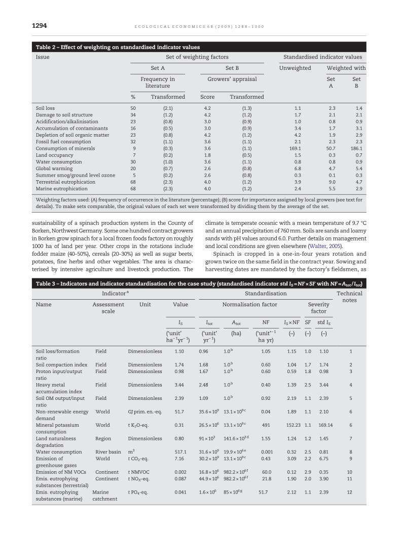
Table 2 – Effect of weighting on standardised indicator values

Issue Set of weighting factors Standardised indicator values

Set A Set B Unweighted Weighted with

Frequency inliterature

Growers' appraisal SetA

SetB

% Transformed Score Transformed

Soil loss 50 (2.1) 4.2 (1.3) 1.1 2.3 1.4Damage to soil structure 34 (1.2) 4.2 (1.2) 1.7 2.1 2.1Acidification/alkalinisation 23 (0.8) 3.0 (0.9) 1.0 0.8 0.9Accumulation of contaminants 16 (0.5) 3.0 (0.9) 3.4 1.7 3.1Depletion of soil organic matter 23 (0.8) 4.2 (1.2) 4.2 1.9 2.9Fossil fuel consumption 32 (1.1) 3.6 (1.1) 2.1 2.3 2.3Consumption of minerals 9 (0.3) 3.6 (1.1) 169.1 50.7 186.1Land occupancy 7 (0.2) 1.8 (0.5) 1.5 0.3 0.7Water consumption 30 (1.0) 3.6 (1.1) 0.8 0.8 0.9Global warming 20 (0.7) 2.6 (0.8) 6.8 4.7 5.4Summer smog/ground level ozone 5 (0.2) 2.6 (0.8) 0.3 0.1 0.3Terrestrial eutrophication 68 (2.3) 4.0 (1.2) 3.9 9.0 4.7Marine eutrophication 68 (2.3) 4.0 (1.2) 2.4 5.5 2.9

Weighting factors used: (A) frequency of occurrence in the literature (percentage); (B) score for importance assigned by local growers (see text fordetails). To make sets comparable, the original values of each set were transformed by dividing them by the average of the set.

1294 E C O L O G I C A L E C O N O M I C S 6 8 ( 2 0 0 9 ) 1 2 8 8 – 1 3 0 0

sustainability of a spinach production system in the County ofBorken,NorthwestGermany.Someonehundredcontractgrowersin Borken grow spinach for a local frozen foods factory on roughly1000 ha of land per year. Other crops in the rotations includefodder maize (40–50%), cereals (20–30%) as well as sugar beets,potatoes, fine herbs and other vegetables. The area is charac-terised by intensive agriculture and livestock production. The

Table 3 – Indicators and indicator standardisation for the case s

Indicator a

Name Assessmentscale

Unit Value

IS

(‘unit’ha−1yr−1)

(

Soil loss/formationratio

Field Dimensionless 1.10 0.9

Soil compaction index Field Dimensionless 1.74 1.6Proton input/outputratio

Field Dimensionless 0.98 1.6

Heavy metalaccumulation index

Field Dimensionless 3.44 2.4

Soil OM output/inputratio

Field Dimensionless 2.39 1.0

Non-renewable energydemand

World GJ prim. en.-eq. 51.7 35

Mineral potassiumconsumption

World t K2O-eq. 0.31 26

Land naturalnessdegradation

Region Dimensionless 0.80 91

Water consumption River basin m3 517.1 31Emission ofgreenhouse gases

World t CO2-eq. 7.16 30

Emission of NM VOCs Continent t NMVOC 0.002 16Emis. eutrophyingsubstances (terrestrial)

Continent t NOX-eq. 0.087 44

Emis. eutrophyingsubstances (marine)

Marinecatchment

t PO4-eq. 0.041 1.6

climate is temperate oceanic with a mean temperature of 9.7 °Candanannual precipitationof 760mm.Soils are sandsand loamysandswith pH values around 6.0. Further details onmanagementand local conditions are given elsewhere (Walter, 2005).

Spinach is cropped in a one-in-four years rotation andgrown twice on the same field in the contract year. Sowing andharvesting dates are mandated by the factory's fieldsmen, as

tudy (standardised indicator std IS=NF×SF with NF=Atot / Itot)

Standardisation Technicalnotes

Normalisation factor Severityfactor

Itot Atot NF IS×NF SF std IS

‘unit’yr−1)

(ha) (‘unit’−1

ha yr)(–) (–) (–)

6 1.0b 1.05 1.15 1.0 1.10 1

8 1.0b 0.60 1.04 1.7 1.74 27 1.0b 0.60 0.59 1.8 0.98 3

8 1.0b 0.40 1.39 2.5 3.44 4

9 1.0b 0.92 2.19 1.1 2.39 5

.6×109 13.1×109c 0.04 1.89 1.1 2.10 6

.5×106 13.1×109c 491 152.23 1.1 169.14 6

×103 141.6×103d 1.55 1.24 1.2 1.45 7

.6×109 19.9×106e 0.001 0.32 2.5 0.81 8

.2×109 13.1×109c 0.43 3.09 2.2 6.75 9

.8×106 982.2×106f 60.0 0.12 2.9 0.35 10

.9×106 982.2×106f 21.8 1.90 2.0 3.90 11

×106 85×106g 51.7 2.12 1.1 2.39 12

Notes to Table 3:Severity factors were taken from Walter and Stützel (2009-this issue). For details on indicator calculation refer to Supplementary data.Technical notes

1. Underlying goal: Protect soil fertility. Target: Erosion rate less than soil formation rate. Data source and method: Owncalculations ( Table A.1, Supplementary data), erosion rates after Universal Soil Loss Equation (Renard et al., 1997)as adapted for Germany by Schwertmann et al. (1987) and Hennings (2000). Soil formation rates of 1 t ha−1 yr−1

assumed (average rates given by Troeh et al., 1998).2. Underlying goal: Protect soil fertility. Target: No exceedance of soil mechanical resistance (equivalent to pressure at

which, at given soil moisture, soil pore volume declines below 8% (Drew, 1992; Horn et al., 1996; Paul, 1999)Data source: Own calculations ( Table A.2, Supplementary data); expert judgement (Uppenkamp, 2003,pers. comm.); machinery and tyre specifications from manufacturers' catalogues.

3. Underlying goal: Protect soil fertility. Target: Proton input rate less than proton output rate. Data source: Owncalculations ( Table A.3, Supplementary data). Fertiliser use and nutrient off-take from official local statistics(LDS, 2001; LK WL, 2002) and expert judgement (Ferdinand Pollert, 2003, pers. comm.). Atmospheric depositionrates of acidifying substances from EMEP, 2002b.

4. Underlying goal: Protect soil fertility. Target: Input rates of Cd, Cr, Cu, Hg, Ni, Pb and Zn less than their output rates.Data source: Own calculations ( Table A.4, Supplementary data), fertiliser use and yield data from official localstatistics (LDS, 2001; LK WL, 2002) and expert judgement (Ferdinand Pollert, 2003, pers. comm.). Plant heavymetal uptake from own data, Bergmann (1992), Delschen and Leisner-Saaber (1998), and UBA (2001).Atmospheric deposition and leaching rates of heavy metals from UBA (2001) and EMEP (2002b).

5. Underlying goal: Protect soil fertility. Target: Soil organic matter (SOM) decomposition rate less than input rate.Data source: Own calculations ( Table A.5, Supplementary data), SOM losses and reproduction fromLeithold et al. (1997). Organic fertiliser use, yields and harvest residues from official statistics (LDS, 2001; LK WL, 2002)and expert judgement (Ferdinand Pollert, 2003, pers. comm.).

6. Underlying goal: sustainable resource use (i.e. prevent rapid and total depletion). Target: Consumption ratedecreasing at a decennial rate to 90% of the previous decade (base-line year 1999). Based on the premisethat (a) a sustainable use would not allow for complete depletion and (b) extraction should be phased outsubsequently (power law) to allow for substitution or other adjustment (Dresselhaus and Thomas, 2001).Data source: Energy consumption from EIA (2001), K consumption from USGS (2001). No mineral P fertiliserused in case study system. Lime reserves are vast and therefore not regarded limiting to sustainability.

7. Underlying goal: Nature conservation (leave habitat/land resources to wildlife). Target: Diverse cultural landscapecapable of sustaining human land use and biodiversity as defined by SRU (1985, 1994), i.e. 10% (semi-) naturalhabitat within a diverse landscape with largely extensive agriculture. Data source: Naturalness DegradationPotential for different land uses from Brentrup et al. (2002), landscape type and infra-structure data from officialstatistics (LDS, 2001; Kreis Borken, 2002).

8. Underlying goal: Nature conservation (leave habitat/resources to wildlife). Target: Human water abstraction notthreatening ecological water flow requirement as defined by Smakhtin et al. (2004). Data source: German waterconsumption assumed representative for the total Rhine-Maas catchment area. Human population figures incatchment from WRI (2003b), multiplied with Per capita water consumption from UBA (2002).

9. Underlying goal: Stop global warming. Target: Reduce energy related greenhouse gas emissions to stabiliseatmospheric CO2-concentrations at 450 ppmv in 2100 (cf. IPCC, 2001).Data source: Global CO2 emissions fromfossil fuel combustion and cement manufacturing from WRI (2003a). Global N2O and CH4 emission estimatesfrom EDGAR (1995 data; changes between 1995 and 2000 are considered negligible; Olivier et al., 2002).(CO2 emission from the decomposition of soil organic matter not included due to lack of consistent data).

10. Underlying goal: Protect human health, prevent vegetation damage.Target: For human health protection:Less than 0.1 ppm hours exceedance of AOT60 (8-hour average) (WHO-EH; Amann and Lutz, 2000). The target toprevent vegetation damage was assumed met if that for human health is met (Amann and Lutz, 2000).Data source: NMVOC emission from EMEP (2002b).

11. Underlying goal: Protect sensitive terrestrial ecosystems. Target: Exceedance of critical loads critical loads inless than 5% of ecosystems (Posch et al., 1995; UBA, 1996).Data source: NH3 and NOX emission from EMEP (2002b).

12. Underlying goal: Protect sensitive aquatic ecosystems. Target: Reduction of nutrient input by 50%, as comparedto 1985 (CONSSO, 2002). Data source: North Sea catchment N and P emissions calculated from per ha emission data(EEA, 2000) and catchment size information (OSPAR, 2000) (1990s data). Atmospheric N deposition (1998 data)fromEMEP (2002a). Target levels for freshwater ecosystemswereassumed tobemet if those formarineecosystemsaremet.

a Refer to Annex I for indicator descriptions.b On-site impacts referenced to one ha of specific land use.c Global land area (excluding permanent ice. FAO, 2001; Olson et al., 1983).d Land area of County of Borken (LDS, 2001).e Land area of Rhine-Maas basin (WRI, 2003b).f Land area of Europe (including Russian Federation West of Urals; FAO, 2001).g Land area of North Sea catchment (OSPAR, 2000).

1295E C O L O G I C A L E C O N O M I C S 6 8 ( 2 0 0 9 ) 1 2 8 8 – 1 3 0 0

1296 E C O L O G I C A L E C O N O M I C S 6 8 ( 2 0 0 9 ) 1 2 8 8 – 1 3 0 0

are amount and timing of fertilisation and pest controlmeasures. Contract growers are responsible for carrying outall cropmanagementmeasures and for irrigation. Harvest andtransportation are contracted to a third party company, onbehalf of the factory. Fertilisation is carried out after soiltesting; pest control follows an integrated pest management(IPM) scheme. A nitrogen base dressing is applied as liquidsprayed fertiliser (urea ammonium-nitrate solution); topdressings are applied as calcium ammonium-nitrate. Usually,no P is applied, because of high soil P content as aconsequence of intensive manuring. Herbicides are usuallyapplied in repeated split rates to increase efficacy. Insecti-cides, if necessary, are selected to minimise environmentalimpacts. Fungicides are not applied. Resistant varieties arecropped during periods of high pressure from downy mildew.

Contracts are made with each individual grower for aparticular field on a yearly basis. During the contract year theygrant the factory's fieldsmen control of crop management.However, between contract years, the factory has little controlover land management. Because of this there is a particularinterest to assess the impact of the single crop spinach onsustainability (rather than that of the full rotation).

3.2. Methods and data

Due to the scope of the study only environmental impacts wereassessed, but the approach can be extended to social andeconomic impacts analogously. Relevant environmental issueswere identified through a structured inventory of potentialissues from the literature, followed by a systematic selection forrelevance within the actual context (Walter and Stützel, 2009-this issue). Severity factors, such as the ones described above,were used as a decision criterion in this selection. Issues with aseverity factor less than one were judged irrelevant foragricultural production in the County of Borken; the ones witha factor greater than onewere classified as relevant. Along withthe set of environmental impact indicators given in Table 1,three economical impact indicators (cost, labour and risk), aswell as yield, were recorded. These three indicators were,however, not standardised and valuated.

We used a simple inventory model (see Supplementarydata for details) to generate the input data for indicatorcalculation. Fig. 2 shows the scope of the inventory; severityfactors were taken from paper I of this series (Walter andStützel, 2009-this issue) and are documented there in detail.Some issues were not represented due to lack of suitable orpracticable indicators. They include human exposure topesticides and emission of noise and odours. The risk ofpesticide use with regard to ecotoxicity and human exposurewas evaluated after Burth et al. (2002) and Gutsche and Enzian(2002), and classified as not being relevant according to theabove criterion (see paper I, Walter and Stützel, 2009-thisissue).

Environmental indicators are usually subject to rather highuncertainty; e.g. due to poor data quality; natural variabilitybetween objects; measurement and model errors; and incom-plete knowledge about the phenomena under investigation.To explore the propagation of uncertainties associated withthe input data, a stochastic simulation approach (cf. IPCC,2000) was used to calculate uncertainty ranges for three of the

standardised indicators: soil erosion, marine eutrophicationand greenhouse gas emissions. Uncertainty ranges of theinput data to these indicators were taken from the originaldata sources. Analysis was limited to these three indicatorsbecause information on input data uncertainty was unavail-able for the others. Triangular distributions (Johnson andKotz, 1999) were used as an (finite interval) approximationof the true (but unknown and semi-finite interval) proba-bility density function for each input variable (cf. Johnson,1997).

Calculations were carried out with the GenStat sta-tistical software package (GenStat Committee, 2003). Foreach indicator, 10,000 values were generated. Uncertaintyranges, defined as the interval between the 2.5% and the97.5% percentile, were then determined from the resultingdistribution.

To assess the impact of introducing a weighting step intothe evaluation scheme, we used two (imaginary) sets ofweighting factors (Table 2). Set A is based on the frequencyby which issues are named in a sample of 44 publications onsustainable agriculture (see paper I, Walter and Stützel, 2009-this issue). Set B is based on the appraisal of five spinachcontract growers who had been involved in a sustainabilityproject for three years andwere asked to score the importanceof the issues listed in Table 1 on a 1 to 5 scale. Means of thescores between the five growers are used as weighting factorshere. For Set A, the percentage of references that appraised aparticular issue as relevant to sustainable agriculture wastaken as a weighting factor. Tomake the two sets comparable,each set was transformed by dividing the individual values bythe average of the particular set, i.e. the transformed weight-ing factors are centred around 1.0.

Note that the weighting factor sets used are by nomeans representative and have not been agreed amongany group of societal actors. They simply resemble ‘weightingfactor sets as they could be’, which are simply used to testthe sensitivity of evaluation results to different weightingschemes.

3.3. Case study results and discussion

Table 3 shows the normalisation and severity factors used, thestandardised indicators, and the sustainability valuationresults.

Among the standardised indicator values, the high valuefor mineral K consumption stands out. It is due to the veryhigh normalisation factor, which reflects the fact thatagriculture consumes much more K than other land uses(the same would apply to P if P fertilisers were applied in theproduction system). On the one hand, a high value forresource consumption seems justified in the light of dimin-ishing fossil, mineral and metal resources, vis-à-vis a growingglobal demand. Agriculture is the single dominant user ofmineral P and K (e.g. in the US, it consumes over 90% of thetotal P and K production; USGS, 2001). At present rates ofconsumption the known economically exploitable reserves ofP and K will be depleted in 90 and 320 years respectively.Replenishing P and K plays a critical role in maintaining soilfertility and hence agricultural production, which provides forover 99% of the human diet (Vitousek et al., 1997). On the other

Table 4 – Uncertainty ranges of the non-standardised andstandardised indicator values of three indicators, derivedby stochastic simulation

Indicator Uncertainty ranges (%)

Non-standardised

Standardised

Indicatorvalue

Indicator value

Lower Upper Lower Upper

Soil loss/formation ratio −30 +30 −65 +55Emission of greenhouse gases −40 +20 −30 +100Emission of eutrophyingsubstances (aquatic)

−50 +70 −65 +230

1297E C O L O G I C A L E C O N O M I C S 6 8 ( 2 0 0 9 ) 1 2 8 8 – 1 3 0 0

hand, any indicator value that is two to three orders ofmagnitude higher than the others – as is the one for resourceconsumption here – may distort results, as they make otherissues look irrelevant by comparison.

The results here highlight that there may be factors otherthan the severity of an issue that wewant to take into account,such as the timeliness of the effects. For instance, wemay ratethe ecotoxicity of pesticides now as more important than thedepletion of mineral resources in a few decades’ time.Technically, this can be achieved by inserting additionalweighting factors into the equation. For example, Bossel(1999) uses dimensionless indicators that relate respite timeto response time. Adding a ‘respite time-to-response timeratio’ would lead to a more realistic assessment of relativeurgency. Additional weighting factors such as this can easilybe integrated into our method.

Further, our analysis shows that the spinach productionsystem in the County of Borken strongly contributes to globalwarming and eutrophication and impairs soil quality. Furtheranalysis of these impacts reveals that nearly 75% of thesystem's global warming potential stems from fertilisation(half direct field emissions from lime application and Nfertilisation and half indirect emissions from fertiliser produc-tion and distribution). The remaining greenhouse gases stemfrom production and maintenance of agricultural machin-ery (∼15%) and diesel and electricity requirements for fieldoperations (∼10%).

Two thirds of the terrestrial eutrophication potential is dueto field NH3 emissions. Diesel combustion and field emissionsof NO each contribute another 10%. Nearly 70% of the marineeutrophication is due to field NO3 losses and 30% from field Plosses. The re-deposition of gaseous emissions plays anegligible role.

Heavy metal accumulation has been recognised as a majorlong-term threat to arable soils in Germany (UBA, 2001; UMK-AMK-LABO-AG, 2000), with copper, zinc and lead being themost critical ones. The metals in danger of accumulation inthe studied spinach system are: chromium, which originatesalmost entirely from lime fertilisers; and lead, originatinghalf from calcium ammonium nitrate fertiliser and half fromlime.

Soil organic matter decomposition in spinach is due tointense cultivation (ploughing two times a year, cultivator use)in combination with lacking organic fertilisation. Soil compac-tion is mainly (70%) caused by narrow and high pressure tyresused to apply fertilisers and spray.

We again emphasise that the method presented here doesnot allow for statements on the overall sustainability of thewhole land uses system. First of all, the sustainability valuationtakes place on the level of the individual indicator. Second, themethod concentrates on negative impacts and does notquantify positive contributions (e.g. maintenance of culturallandscapes through agriculture). If these positive contributionswere conceptualised as benefits and the negative impacts ascosts, we might find these costs quite acceptable compared tothe produced benefits. The fact that single indicators of theanalysed system are in the unsustainable realm should thus beinterpreted as an indication of action hot spots, but it does notallow for inferences on the whole system's sustainability orunsustainability.

In the case study, the normalisation factors, NF, showmuch greater spread than the severity factors, SF. The finalstandardised indicator values are highly correlated with thenormalised indicator values, IS×NF, but show no correlationwith the severity factors.

The same is true for the weighting factors, as Table 2shows: The weighted results are highly correlated with theunweighted ones (rN0.99). (This correlation is supported bythe large value pairs for K consumption. Deleting theseextreme values, weighted and un-weighted values are stillcorrelated with r=0.94 and r=0.64 for weighting factor sets Aand B respectively).

Interestingly, both weighting factor sets largely concur inwhich issues aremore andwhich ones are less important thanthe average. Both sets judge soil compaction, fossil fuelconsumption, water consumption and eutrophication asmore important than the average, and soil acidification,heavy metal accumulation, land occupancy, global warmingand ground level ozone as less important than the average.Only two of twelve issues – soil organic matter depletion andmineral K consumption – are judged differently in the two setsof weighting factors. In both cases, the weighting based on thefrequency of occurrence in the literature leads to lower-than-average weighting, and the farmers’ appraisal to higher-than-average weighting.

The uncertainty ranges for the standardised indicators,obtained by stochastic simulation, are shown in Table 4. For allthree indicators, the uncertainty of the standardised value (stdIS) was by a factor of 2.0 to 2.5 higher than that of the non-standardised indicator value (IS). Although these resultscannot be extrapolated to the other indicators, for which nosimulations were carried out, they do indicate that thestandardisation procedure inflates uncertainty substantially.As tracking the uncertainty through the standardisationprocess reveals, this inflation of uncertainty was mainlycaused by the division operations, especially where theuncertainty of divisors was high.

Acknowledgements

This work was funded through the Unilever SustainableAgriculture Programme, with in-kind support from the

1298 E C O L O G I C A L E C O N O M I C S 6 8 ( 2 0 0 9 ) 1 2 8 8 – 1 3 0 0

Horticultural Extension Service of the Chamber of AgricultureNorthrhine-Westphalia.

The authors would like to thank Olaf Christen, RobertCostanza and Hartmut Bossel and Frank Brentrup for inspiringdiscussions and helpful comments on an earlier version ofthis paper; Stefan Krusche for programming the stochasticsimulations in GenStat; the Iglo field staff and pilot growers forreality checking the data; and Vanessa J. King and Rachael A.Durrant for proof reading and checking the English.

Appendix A. Supplementary data

Supplementary data associated with this article can be found,in the online version, at doi:10.1016/j.ecolecon.2008.11.017.

R E F E R E N C E S

Amann, M., Lutz, M., 2000. The revision of air quality legislation inthe European Union related to ground-level ozone. Journal ofHazardous Materials 78, 41–62.

Amann, M., Imrich, B., Cofala, J., Gyarfas, F., Klimont, Z., Schöpp,W., 1999. Integrated assessment modelling for the protocol toabate acidification, eutrophication and ground-level ozone inEurope. Report to the Dutch Ministry of Housing, SpatialPlanning and Environment. International Institute for AppliedSystems Analysis (IIASA), Laxenburg.

Bergmann, W. (Ed.), 1992. Nutritional Disorders of Plants. GustavFischer, Jena.

Bockstaller, C., Girardin, P., van der Werf, H.M.G., 1997. Use ofagro-ecological indicators for the evaluation of farmingsystems. European Journal of Agronomy 7, 261–270.

Bossel, H., 1999. Indicators for Sustainable Development: Theory,Method, Applications. IISD, Winnipeg.

Brentrup, F., Küsters, J., Lammel, J., Kuhlmann, H., 2002. Life CycleImpact Assessment of land use based on the Hemerobyconcept. International Journal of Life Cycle Assessment 7,339–348.

Brentrup, F., Küsters, J., Lammel, J., Kuhlmann, H., 2004.Environmental impact assessment of agricultural productionsystems using the life cycle assessment methodology — I.Theoretical concept of a LCA method tailored to cropproduction. European Journal of Agronomy 20, 247–264.

Burth, U., Gutsche, V., Freier, B., Roßberg, D., 2002. Das notwendigeMaß bei der Anwendung chemischer Pflanzenschutzmittel(with English abstract). Nachrichtenblatt des DeutschenPflanzenschutzdienstes 54, 297–303.

Christen, O., 1999. Sustainable agriculture — from the history ofideas to practical application. Institut für Landwirtschaft undUmwelt (ilu), Bonn.

CONSSO, 2002. Fifth International Conference on the Protection ofthe North Sea. Progress Report. Committee of North Sea SeniorOfficials (CONSSO), Bergen.

Costanza, R., 1993. Developing ecological research that isrelevant for achieving sustainability. Ecological Applications3, 579–581.

Delschen, T., Leisner-Saaber, J., 1998. Selbstversorgung mitGemüse aus schwermetallbelasteten Gärten: EineGefährdungsabschätzung auf toxikologischer Basis (inGerman, with English abstract). Bodenschutz 1/98, 17–20.

Dresselhaus, M.S., Thomas, I.L., 2001. Alternative energytechnologies. Nature 414, 332–337.

Drew, M.C., 1992. Soil aeration and plant root metabolism. SoilScience 154, 259–269.

Eckert, H., Breitschuh, G., Sauerbeck, D.R., 2000. Criteria andstandards for sustainable agriculture. Journal of Plant Nutritionand Soil Science 163, 337–351.

EEA, 2000. Environmental Signals 2000— Regular Indicator Report.European Environment Agency (EEA), Copenhagen.

EIA, 2001. International Energy Annual, Release 2001. Website ofthe U.S. Energy Information Administration (EIA) (http://www.eia.doe.gov/emeu/international/).

EMEP, 2002a. Emission data reported to UNECE/EMEP. MSC-WStatus Report 2002. EMEP/MSC-W, Blindern.

EMEP, 2002b. Online Database (WebDaB 2002). http://webdab.emep.int. 2nd release. EMEP/MSC-W, Blindern.

FAO, 2001. FAOSTAT: FAO Statistical Databases. (available athttp://www.fao.org/waicent/portal/ statistics_en.asp). Foodand Agriculture Organisation of the United Nations (FAO),Rome.

Ferm, M., 1998. Atmospheric ammonia and ammonium transportin Europe and critical loads — a review. Nutrient Cycling inAgroecosystems 51, 5–17.

Fields, C.B., 2001. Sharing the garden. Science 294, 2490–2491.Funtowicz, S.O., Ravetz, J.R., 1993. Science for the post-normal age.

Futures 25, 739–755.GenStat Committee, 2003. GenStat® Release 7.1: Reference

Manual. VSN International, Oxford.Gutsche, V., Enzian, S., 2002. Quantifizierung der Ausstattung einer

Landschaft mit naturbetonten terrestrischen Biotopen auf Basisdigitaler topographischer Daten (German, with Englishabstract).NachrichtenblattdesDeutschenPflanzenschutzdienstes54, 92–101.

Halberg, N., 1999. Indicators of resource use and environmentalimpact for use in a decision aid for Danish livestock farmers.Agriculture, Ecosystems and Environment 76, 17–30.

Hansen, J.W., 1996. Is agricultural sustainability a useful concept?Agricultural Systems 5, 117–143.

Hennings, V. (co-ordinator), 2000. MethodendokumentationBodenkunde: Auswertungsmethoden zur Beurteilung derEmpfindlichkeit und Belastbarkeit von Böden (in German). E.Schweizerbart'sche Verlagsbuchhandlung, Hannover.

Horn, R., Paul, R., Simota, C., Fleige, H., 1996. Schutz vormechanischer Belastung (in German). In: Blume, H.-P. (Ed.),Handbuch der Bodenkunde, Kap 7.4 (14. Erg. Lfg. 12/2002).ecomed, Landsberg (Lech), pp. 1–12.

Hoyningen-Huene, P., 1999. The nature of science. Nature andResources 35, 4–8.

IPCC, 2000. Good Practice Guidance and Uncertainty Managementin National Greenhouse Gas Inventories. IntergovernmentalPanel on Climatic Change (IPCC). Geneva.

IPCC, 2001. IPCC Third Assessment Report— Climate Change 2001.Intergovernmental Panel on Climatic Change (IPCC). Geneva.

Izac, A.-M.N., Swift, M.J., 1994. On agricultural sustainability andits measurement in small-scale farming in sub-Saharan Africa.Ecological Economics 11, 105–125.

Jamieson, D., 1998. Sustainability and beyond. EcologicalEconomics 24, 183–192.

Johnson, D., 1997. The triangular distribution as a proxy for thebeta distribution in risk analysis. The Statistician 46,387–398.

Johnson, N.L., Kotz, S., 1999. Non-smooth sailing or triangulardistributions revisited after some 50 years. The Statistician 48,179–187 part 2.

LDS, 2001. Statistisches Jahrbuch Nordrhein-Westfalen 2001 (inGerman). Landesamt für Datenverar-beitung und StatistikNordrhein-Westfalen (LDS), Düsseldorf.

Leithold, G., Hülsbergen, K.-J., Michel, D., Schönmeier, H., 1997.Humusbilanzierung — Methoden und Anwendungen alsAgrar-Umweltindikator. In: Diepenbrock, W., Kaltschmitt, M.,Nieberg, H., Reinhardt, G.A. (Eds.), UmweltverträglichePflanzenproduktion – Indikatoren, Bilanzierungsansätze undihre Einbindung in Ökobilanzen – Fachtagung am 11. und 12.

1299E C O L O G I C A L E C O N O M I C S 6 8 ( 2 0 0 9 ) 1 2 8 8 – 1 3 0 0

Juli 1996 in Wittenberg. Schriftliche Fassung der Beiträge.Zeller, Osnabrück, pp. 43–54.

LK WL, 2002. Zahlen in Westfalen-Lippe (2000–2002)(in German). Landwirtschaftskammer West-falen-Lippe (LKWL), Münster.

Ludwig, D., Hilborn, R., Walters, C., 1993. Uncertainty, resourceexploitation, and conservation: Lessons learned from history.Science 260 (17), 36.

Kreis Borken, 2002. Region, Zahlen, Fakten. Kreis Borken.Matson, P.A., Parton, W.J., Power, A.G., Swift, M.J., 1997. Agricultural

intensification and ecosystem properties. Science 277, 504–509.Mosier, A.R., 2001. Exchange of gaseous nitrogen compounds

between agricultural systems and the atmosphere. Plant andSoil 228, 17–27.

Müller-Wenk, R., 1996. Political and scientific targets indistance-to-target valuation methods. In: Braunschweig, A.,Förster, R., Hofstetter, P., Müller-Wenk, R. (Eds.), Developmentsin LCA Valuation. IWÖ-Diskussionsbeitrag 32. Institut fürWirtschaft und Ökologie, St. Gallen.

Niu, W.-Y., Lu, J.J., Khan, A.A., 1993. Spatial systems approach tosustainable development: a conceptual frameworkEnvironmental Management 17, 179–186.

OECD, 1998. Environmental Indicators. Towards SustainableDevelopment. Organisation for Economic Co-operation andDevelopment (OECD), Paris.

OECD, 2000. Environmental Indicators for Agriculture. Methodsand Results. Organisation for Economic Co-operation andDevelopment (OECD), Paris.

Olivier, J.G.J., Berdowski, J.J.M., Peters, J.A.H.W., Bakker, J.,Visschedijk, A.J.H., Bloos, J.P.J., 2002. Applications of EDGAR.Including a description of EDGAR 3.2: reference database withtrend data for 1970–1995. RIVM, Bilthoven. RIVM Report 773301001/NRP Report 410200 051. Available online at http://www.mnp.nl/en/publications/2002/Applications_of_EDGAR_Emission_Database_for_Global_Atmospheric_Research.html.

Olson, J.S., Watts, J.A., Allision, L.J., 1983. Carbon in Live Vegetationof Major World Ecosystems. Environmental Science Division,Publication No. 1997. Oak Ridge National Laboratory (ORNL),Oak Ridge, TN.

OSPAR, 2000. Quality Status Report 2000. OSPAR Commission,London.

Paul, R., 1999. Zur Verdichtungsgefährdung im Rahmen desBodengefügeschutzes auf großen Flächen (in German)Kolloquium “Einfluß der Großflächen-Landwirtschaft auf denBoden”. Thüringer Ministerium für Landwirtschaft,Naturschutz und Umwelt. Jena, 6 May 1999.

Calculation and mapping of critical thresholds in Europe. In:Posch, M., de Smet, P.A.M., Hettelingh, J.-P., Downing, R.J. (Eds.),Status Report 1995. Coordination Center for Effects (CCE),RIVM, Bilthoven.

Reganold, J.P., Glover, J.D., Andrews, P.K., Hinman, H.R., 2001.Sustainability of three apple production systems. Nature 410,926–929.

Renard, K.G., Foster, G.R., Weesies, G.A., McCool, D.K., Yoder, D.C.(Eds.), 1997. Predicting Soil Erosion by Water: A Guide toConservation Planning with the Revised Universal Soil LossEquation (RUSLE). USDA-ARS, Washington, DC.

Sands, G.R., Podmore, T.H., 2000. A generalized environmentalsustainability index for agricultural systems. Agriculture,Ecosystems and Environment 79, 29–41.

Schäfer, D., Schoer, K., Seibel, S., Zieschank, R., Barkmann, J.,Baumann, R., Meyer, U., Müller, F., Lehniger, K., Steiner, M.,Wiggering, H., 2002. Makroindikatoren des Umweltzustandes(in German). Beiträge zu den UmweltökonomischenGesamtrechnungen, Band 10. Statistisches Bundesamt.Metzler-Poeschel, Wiesbaden.

Schwertmann, U., Vogl, W., Kainz, M., 1987. Bodenerosion durchWasser — Vorhersage des Ab-trags und Bewertung vonGegenmaßnahmen. Ulmer, Stuttgart.

Smakhtin, V., Revenga, C., Döll, P., 2004. A pilot global assessmentof environmental water requirements and scarcity. WaterInternational 29, 307–317.

Smith, C.S., McDonald, G.T., 1998. Assessing the sustainability ofagriculture at the planning stage. Journal of EnvironmentalManagement 52, 12–37.

Smyth, A.J., Dumanski, J., 1995. A framework for evaluatingsustainable land management. Canadian Journal of SoilScience 75, 401–406.

SRU, 1985. Sondergutachten 1985: Umweltprobleme derLandwirtschaft (in German). Der Rat von Sachverständigen fürUmweltfragen (SRU). W. Kohlhammer, Stuttgart.

SRU, 1994. Umweltgutachten 1994 des Rates vonSachverständigen für Umweltfragen: Für eine dauerhaft-umweltgerechte Entwicklung. Metzler-Poeschel, Stuttgart. (inGerman, English excerpts published as SRU: Envrionmentalreport 1994: In pursuit of sustainable environmentally sounddevelopment. available via http://www.umweltrat.de).

Stevenson, M., Lee, H., 2001. Indicators of sustainability as a tool inagricultural development: partitioning scientific andparticipatory processes. International Journal of SustainableDevelopment and World Ecology 8, 57–65.

Stockle, C.O., Papendick, R.I., Saxton, K.E., Campbell, G.S., vanEvert, F.K., 1994. A framework for evaluating the sustainabilityof agricultural production systems. American Journal ofAlternative Agriculture 9, 45–50.

Syers, J.K., Hamblin, A., Pushparajah, E., 1995. Indicators andthresholds for the evaluation of sustainable landmanagement.Canadian Journal of Soil Science 75, 423–428.

Tacconi, L., 1998. Scientific methodology for ecological economics.Ecological Economics 27, 91–105.

Tilman, D., Reich, B.P., Knops, J., Wedin, D., Mielke, T., Lehman, C.,2001. Diversity and productivity in a long-term grasslandexperiment. Science 294, 843–845.

Troeh, F.R., Hobbs, J.A., Donahue, R.L., 1998. Soil and WaterConservation. Prentice Hall, Upper Saddle River, N.Y.

UBA, 1996. UNECE Manual on methodologies and criteria formapping critical levels/loads and geographical areas wherethey are exceeded. Umweltbundesamt (UBA) Berlin.Available online at: http://www.umweltbundesamt.de/mapping/.

UBA, 2001. Grundsätze und Maßnahmen für einevorsorgeorientierte Begrenzung von Schadstoffeinträgen inlandbaulich genutzte Böden. UBA-Texte 59/01 (in German).Umweltbundesamt (UBA), Berlin.

UBA, 2002. Environmental Data Germany 2002. Umweltbundesamt(UBA), Berlin.

UMK-AMK-LABO-AG, 2000. Cadmiumanreicherung inBöden/Einheitliche Bewertung von Dünge-mitteln (in German).Bericht für die 26. ACK der Umweltministerkonferenz am11./12.10.2000, Bund/Länder-ArbeitsgemeinschaftBodenschutz (LABO), Hamburg.

USGS, 2001. Mineral Commodity Summaries 2001. U.S. GeologicalSurvey (USGS), Washington, DC.

vanMansvelt, J.D., 1997. An interdisciplinary approach to integratea range of agro-landscape values as proposed byrepresentatives of various disciplines. Agriculture, Ecosystemsand Environment 63, 233–250.

Vitousek, P.M., Mooney, H.A., Lubchenco, J., Melillo, J.M., 1997.Human domination of earth's ecosystems. Science 277,494–499.

Wackernagel, M., Yount, J.D., 1998. The ecological footprint: anindicator of progress towards regional sustainabilityEnvironmental Monitoring and Assessment 51, 511–529.

Walter, C. 2005. Sustainability Assessment of Land Use Systems.PhD Dissertation. Institute of Vegetable and Fruit Science,Natural Sciences, University of Hanover, Germany. Availableonline at: http://www.gartenbau.uni-hannover.de/gem/Literatur/index_veroeff.htm.

1300 E C O L O G I C A L E C O N O M I C S 6 8 ( 2 0 0 9 ) 1 2 8 8 – 1 3 0 0

Walter, C., Stützel, H., 2009. A New Method for Assessing theSustainability of Land-Use Systems (I): Identifying the RelevantIssues. Ecological Economics 68, 1275–1287 (this issue).

WRI, 2003a. Carbon Emissions from Energy Use and CementManufacturing, 1850 to 2000. World Resources Institute (WRI),Washington, DC. Available on-line through the ClimateAnalysis Indicators Tool (CAIT) at: http://cait.wri.org.

WRI, 2003b. Watersheds of the World_CD. World ConservationUnion (IUCN), International Water Management Institute(IWMI), Ramsar Convention Bureau, and World ResourcesInstitute (WRI), Washington, DC. Available online at: http://www.iucn.org/themes/wani/eatlas/.