
A New Approach for Routing Courier Delivery
Services with Urgent Demand
Chen Wang
Daniel J. Epstein Department of Industrial and Systems Engineering
University of Southern California
Los Angeles, CA 90089-0193
Fernando Ordonez
Industrial Engineering Department
Universidad de Chile
Republica 701, Santiago, Chile
Maged Dessouky*
Daniel J. Epstein Department of Industrial and Systems Engineering
University of Southern California
Los Angeles, CA 90089-0193
*corresponding author

2
A New Approach for Routing Courier Delivery
Services with Urgent Demand
Abstract
Courier delivery services deal with the problem of routing a fleet of vehicles from
a depot to service a set of customers that are geographically dispersed. In many cases, in
addition to a regular routine demand, the industry is faced with sporadic, tightly
constrained, urgent requests. An example of such an application is the transportation of
medical specimens, where timely, efficient, and accurate delivery is crucial in providing
high quality and affordable patient services. We model this problem as a multi-trip
vehicle routing problem with time windows using stochastic programming with recourse
to represent the random urgent requests. We solve the proposed model with an insertion
based heuristic and a tabu-search improvement component. The solution obtained is a
master plan that solves the first phase of the stochastic programming problem and takes
into account the recourse actions for daily plans given specific customer occurrence. We
evaluate the model and solution strategy through simulations on randomly generated data
as well as on a real data set provided by a leading healthcare provider in Southern
California. We find that our solution obtains significant improvement in travel costs as
well as in quality of service as measured by route similarity over existing methods.
Keywords:
Stochastic vehicle routing; Multi-trip; Time windows; Urgent demand; Insertion; Tabu
Search

3
1. Introduction
In this study, we consider a stochastic vehicle routing problem with urgent
demand. This variant of the routing problem is a common problem in the courier delivery
industry, as the industry is faced with uncertain demands, as well as sporadic, tightly
constraint, and urgent requests. One example application of the problem is the
transportation of clinical specimens, which is pervasive in the healthcare industry. On a
daily basis, millions of specimens are delivered in the United States from dispersed
hospitals and clinics to centralized laboratories for testing and reporting. Timely and
efficient transportation of specimens is crucial in providing high-quality and affordable
patient service in the healthcare industry. The current situation, however, is far from
ideal, where lost or delayed delivery of specimen is the most common problem
jeopardizing patient safety (Astion et al, 2003). Additionally, the cost on the
transportation of clinical specimens is a significant burden to healthcare systems,
especially for urgent cases which require prompt courier services.
There are several characteristics in the laboratory courier routing problem that any
routing technique must take into consideration. Because of the perishable nature of the
demand and varying levels of urgency for the requests, the clinical specimens generally
fall into two kinds of delivery time windows. The random urgent ones typically need to
be transported within an hour, while the regular routine ones may have up to four hours
of turnaround time. Another characteristic of the laboratory routing system is the two
types of facilities that the testing requests come from, namely hospitals and clinics.
Hospitals normally operate around the clock, whereas clinics typically do not require
service during nights and weekends. For this reason, optimal routing of courier service
will need to take into account the changing demand levels at different time periods.
Even though there are a number of studies and published results in the routing
literature, the scheduling of urgent delivery of medical specimens is still a manual
process in practice. In industry, many of the urgent requests are delivered by an
outsourced courier service, such as taxis while the regular routine requests are serviced
by their own fleet. However, this is extremely costly; especially for a mid-to-large size
system since the outsourcing cost can be rather high. We propose to plan additional

4
capacity in the fleet, which can be used to accommodate the random urgent requests. The
key issue in this problem is how to integrate these uncertain demands into the delivery
schedule for the routine demands. If a chance constraint model or a robust optimization
approach is used, either the unlikely requests are ignored or the solution considering them
is at a high cost. Instead, we use a stochastic programming with recourse approach to
handle the urgent requests. This approach requires a massive number of scenarios,
leading to a large scale routing problem. We propose a two stage stochastic
programming model to take into account the cost of routing urgent requests with that of
routing regular ones. The overall idea is to understand whether we can sacrifice some
optimality with regard to regular demand to free some capacity that will give more
flexible routes, which could accommodate the more urgent requests at a lower cost.
One advantage of the current industry practice, which runs fixed daily routes in
the planning horizon outsourcing most random requests, is that it maintains the similarity
of routes for regular requests with customers visited by the same vehicle at roughly the
same time every day. Such stability is desirable in repeating systems where the quality of
service is important (Groër et al., 2009; Sungur et al., 2010). However, this rigid routing
strategy also has a drawback in that it is inefficient when there is a significant amount of
random urgent demands. In this approach, most of the random urgent specimen bypass
the routing system and are outsourced, at a substantial additional cost.
In this research, we build a model for this vehicle routing problem, and solve it
using heuristic algorithms. The model and the heuristic algorithms take into account the
following characteristics of the healthcare delivery application: continuous demand,
urgent requests, and multiple objectives. The work is built based on the assumption that it
may be possible to satisfy the regular demands in a way that the slack of the regular fleet
can be used to address urgent requests to reduce the use of outsourced vehicles. We build
a multi-trip formulation and use stochastic programming with recourse for the master and
daily routes. When formulating the master plan, it is desirable that the master plan be
similar to the daily plans that have uncertainty in customer occurrence. We use an
approach that forms the master plans that would require little modification when adapted
to daily schedules. Both the master plan and the recourse action for each daily schedule
consider a multi-objective function that minimizes the travel and outsourcing costs, and

5
maximizes the service quality of the healthcare customer as measured by route
similarity.
The rest of the paper is organized as follows. In section 2, a literature review of
the relevant problems is presented. Section 3 introduces the problem formulation. In
section 4, we present our heuristic solution technique for the problem. In section 5,
experimental results of an application of the proposed heuristic on randomly generated
data sets as well as on a real data set from a large healthcare provider in Southern
California are presented and discussed. Conclusions are presented in section 6.
2. Literature Review
The VRP variants related to this work are multi-trip VRP (MVRP) and stochastic
VRP (SVRP). The study is also related to customer services in the vehicle routing
problem. We next present a short summary of the prior work in these areas.
Multi-trip VRP (MVRP), as a variant of the VRP, has gained little attention in the
literature. In the MVRP, vehicles can be used more than once during the planning
horizon. Taillard et al. (1996) suggest in their study that assigning more routes to a
vehicle is a more practical solution in real life. Brandao and Mercer (1997& 1998)
improved the study by considering not multi-trip VRP, but also including the delivery
time window and the capacity of the vehicles. Petch and Salhi (2003) integrate the
approaches proposed by Taillard et al. (1996) and Brandao and Mercer (1997 & 1998).
Azi et al. (2006) first describe an exact algorithm for solving a multi trip VRP problem of
one vehicle with time windows. Salhi and Petch (2007) provide a comprehensive
literature review on the multi-trip VRP, and present a genetic algorithm based on a
heuristic for the solution of MVRP. In recent years, Zapfel and Bogla (2008) provide a
study of a multi-trip vehicle routing and crew scheduling with overtime and outsources
options. Ren et al. (2010) introduce the use of shifts into the VRP, and study a new
variant of the VRP, which is with time windows, multi-shifts, and overtime.
Another variant of the multi-tripVRP is the periodic VRP, which customers have
to be visited once or several times in the planning horizon (Angelelli and Speranza,
6
2002). PVRP extends the classic planning horizon to several days. Angelelli and
Speranza (2002) propose a Tabu search based heuristic for the solution of a PVRP with
intermediate facilities. Francis and Smilowitz (2006) present a continuous approximation
for service choice of a PVRP with capacity constraints. Hemmelmayr et al. (2009)
propose a new heuristic for solving PVRP as well as a Periodic Travelling Salesman
Problem, based on a neighborhood search. The paper of Alonso et al. (2008) extends the
classical VRP to a periodic and multi-trip VRP with site-dependency and proposes a
Tabu search based algorithm.
The stochastic vehicle routing problem (SVRP) introduces uncertainty in the
parameters. Ichoua et al. (2006) reviews the literature in SVRP and classifies the SVRP
into two subgroups of problems: static stochastic vehicle routing problems (SSVRP) and
dynamic stochastic vehicle routing problem (DSVRP). In the SSVRP, the customers
and/or demands are random variables. The vehicle routing problem with stochastic
demand (VRPSD) (e.g., Yang et al., 2000), the vehicle routing with stochastic customer
(VRPSC) (e.g., Waters 1989), the vehicle routing problem with stochastic customer and
demand (VRPSCD) (e.g., Gendreau et al., 1995), and the probabilistic travelling
salesman problem (PTSP) (e.g., Laporte et al., 1994) belong to SSVRP. One typical
solution technique for the SSVRP is the two-stage method (Gendreau et al., 1996;
Bertsimas and Simchi-levi, 1996), where in the first stage, an “a-priori sequence”
solution (Bertsimas et al., 1990) is proposed, and in the second stage, recourse actions
(e.g., skipping non-occurring customers, returning to the depot when capacity is
exceeded, or complete rescheduling for occurring customers) is allowed to adjust an “a-
priori solution” after the uncertainty is revealed. Another solution technique for the
SSVRP is the “re-optimization” approach (e.g., Secomandi, 2001; Novoa and Storer,
2009), where dynamic programming solutions are developed.
DSVRP studies the problems where new events occur over time and no “a-priori”
solution is utilized. There are two different ways to exploit the probability information in
the literature: analytical studies and stochastic algorithms. The analytical studies provide
new insights to the solution structure, thus helps design more efficient deterministic
algorithms (Bertsimas and Simchi-levi, 1996). For problems with uncertainty (e.g.,
Spivey and Powell, 2004), researchers have been studying stochastic and dynamic

7
algorithmic approaches that include current information and future probabilistic events to
produce more efficient solutions.
The healthcare courier delivery problem has a high requirement on the quality of
customer service. Some recent work has included customer service in the models for
fixed route delivery systems under stochastic demand (Haughton and Stenger 1998).
Haughton (2000) develops a framework for quantifying the benefits of route re-
optimization, also under stochastic customer demands. Zhong et al. (2007) propose an
efficient way of designing driver service territories, considering uncertainty in customer
locations and demand. Groër et al. (2009) introduce the Consistent VRP (ConVRP)
model, with an objective of obtaining consistent routs such that the customers are visited
by the same driver at roughly the same time on each day. Sungur et al. (2010) introduce
the concept of “route similarity” as the number of customers of the daily routes that are
within a given distance of any customer on the master plan route, and use it as a key
measure for developing optimal routing strategies.
3. Vehicle Routing with Urgent Requests
We formulate a multi-trip vehicle routing model for the healthcare industry
courier delivery problem, taking into account the efficient scheduling of regular and
urgent requests, as well as route similarities. The primary distinction in the domain of the
multi-trip VRP formulation is that the earlier research on MVRP has discrete operation
periods of equal length for all vehicles, and we allow in this work continuous non-equal
operation periods for different vehicles. For example, a MVRP may require the
customers to be visited twice in two trips in a workday, with a fixed trip length. A PVRP
may have all the customers be visited in one trip each workday during the planning
horizon of a week, where the length of a trip of a vehicle is 8 hours per day. In our
problem, the vehicles operate in multiple trips during the planning horizon; the length of
the trips for each vehicle will not be defined initially, but be flexible based on the time
window of the demands. There are multiple trips with varying length during the planning
horizon because when we have a vehicle to visit a customer for pickup of a medical
specimen, it is required that the specimen should be delivered to the lab by the same

8
vehicle on the same trip. In this section, we provide a mixed integer programming
formulation of this multi-trip VRPTW with stochastic clients.
Assume we are making a routing schedule for a healthcare courier delivery
service provider. There are potential customers (hospitals, clinics) in the region that
must be visited during a planning horizon (say a day) by a fleet of identical vehicles.
Each request for service has a location, pick up time window and delivery deadline. The
locations and time windows of all the potential customers are known ahead of time,
however, which customers have requests on a specific day is only revealed on the day the
requests are made. This uncertainty is represented by a set of scenario days ,
with the scenario for day d occurring with a given probability pd. There is one depot
(node ) located at the central lab. Each vehicle should leave the depot at the beginning
of the day, and return to the depot at the end of the day. It can also return to the lab
anytime during the day when required (i.e., when there are urgent requests that need
samples delivered by a certain time at the lab.). As each vehicle has multiple trips, we
assume a dummy depot (represented by node ) located also at the central lab to
keep track of which trip the request is on. The notation of the model formulation is as
follows.
The routing parameters:
: set of scenario days .
: set of customers, .
: set of vehicles.
: set of daily trips of a vehicle, .
The cost parameters:
: minimum travel time between node and j.
: unit travel cost, dollars per mile.
: unit outsource cost, dollars per taxi trip.
: unit dissimilarity cost, dollars for each count of dissimilarity.
The stochastic parameters:

9
pd: probability of occurrence of scenario day d.
: set of occurring customer requests on scenario day d.
: service time of customer request i on day d.
: the earliest time that the customer can be visited for request i on day d.
: the latest time that the customer can be visited for request i on day d.
: the latest time that the customer request i can be delivered to the lab on day d.
Other parameters:
: a sufficiently large number.
The routing variables:
{
{
{
: the time vehicle k arrives at customer on day d.
: the time that vehicle k leaves the depot for its trip w on day d.
: the time that vehicle k returns to depot from its trip w on day d.
The auxiliary demand variables:
{
{
{
Before the mathematical formulation of the model is presented, some clarification
on the parameters and decision variables need to be made.

10
1) The model considers a horizon of one day with δ=|D|-1 days of demand scenarios
to represent the uncertainty. Day is used to represent the planning for the
master routes.
2) The maximum number of trips each vehicle can make in a day is . We allow
artificial trips that do not deal with any customers, but just “move” from the depot
to the lab and back to the depot without spending any actual time.
3) is the minimum travel time between node and j. Particularly, is the
minimum travel distance between the depot and node i ; is the minimum
travel time between node and the depot.
4) is defined as the measure of dissimilarity, with mathematical expression
∑
∑
. Variable
equals 1 if customer i is visited by
vehicle k either on day d or on day 0, but not both. This variable equals to 0 if
customer is visited by vehicle both on day d and on day 0, or is not visited
either day. In other words the dissimilarity is counted as one if a customer is
visited by a different vehicle than in the master plan.
Problem formulation:
Minimize
∑ ∑(∑ ∑
∑ ∑
∑ ∑
)
∑ ∑
∑ ∑ ∑
(3.1)
Subject to:
Routing constraints:
∑ ∑
∑ ∑
(3.2)
∑
∑
∑
∑
∑
(3.3)

11
∑
∑
(3.4)
∑
∑
(3.5)
( ) (3.6)
(
) (3.7)
( ) (3.8)
(3.9)
(3.10)
(
)
(
) (3.11)
(
) (3.12)
∑
∑
(3.13)
Domain constraints:
(3.14)
(3.15)
(3.16)
(3.17)
(3.18)
(3.19)
(3.20)
(3.21)
(3.22)

12
As previously described, the healthcare courier delivery problem should focus not
only on plans with minimum travelling cost, but also those with high level of customer
service. Therefore, the objective function of our model, as shown in Equation (3.1), is to
minimize the expected total cost, that is composed of traveling cost, outsourcing cost, and
route dissimilarity cost. For brevity, we will use the term “taxi” to refer to an outsourced
vehicle for the remainder of the paper. The travel cost is represented
by ∑ ∑ (∑ ∑
∑ ∑
∑ ∑
), which is the expected total distance traveled by all the vehicles in the planning
horizon. Here we take p0=1 so the objective is actually the cost of the master route and
the expected travel, taxi and dissimilarity cost over the scenario days. The outsourcing
cost is represented by ∑ ∑
, which is the expected number of trips that a
taxi is used to handle the demands unmet by the regular fleet. It should be noted that this
term could easily include the total taxi distance if we change it to
∑ ∑ . The expected route dissimilarity cost is measured by
∑ ∑ ∑
, which is proportional to the total number of customers that are
serviced by a vehicle different from the one servicing it in the master plan.
There are two groups of constraints in our model, namely routing constraints and
domain constraints. Constraint (3.2) assures on each day that each customer should be
visited directly from the depot, right after a vehicle services customer , or by a taxi when
the regular fleet is unavailable. Constraint (3.3) assures that each vehicle must leave the
customer after visiting it. It also addresses the fact that a customer has to be visited by a
vehicle in one of its trips in a day. Constraint (3.4) ensures that each individual trip
should start with leaving the depot and end by returning to the depot. Constraint (3.5)
enforces the usage of early trips as much as possible, which force the empty trips close to
the end of the day instead of at the beginning of the day. Constraint (3.6) assures the
relationship of arrival times at customers and , when customer is visited right after
is visited. Constraint (3.7) expresses the relationship of arrival time to customer , when
is the first customer request a vehicle handles in a trip. Constraint (3.8) expresses the
relationship of arrival time to customer , when is the last customer request a vehicle
handles in a trip. Constraint (3.9) enforces that the finish time of a trip of a vehicle should
be no later than the start time of the next trip of the vehicle. Constraint (3.10) enforces the

13
arrival time of a vehicle at a customer to be in the required time window for handling the
customer request. Constraint (3.11) requires that the arrival time at a customer on a trip
should be between the start time and the end time of the trip. Constraint (3.12) requires
that each vehicle should visit the lab before the drop-off deadline of each specimen
collected by a vehicle on a trip. Constraint (3.13) is another representation of our
expression for dissimilarity ∑
∑
. It removes the usage of the
absolute value in the expression, so that the system is linearized. Constraints (3.14) –
(3.22) are the variable domain constraints.
4. Heuristic
Because of the combinatorial nature of the problem, exact solution methods will
only be able to solve small size instances of this problem. Since there are days that
have to be taken into account in the routing, and each vehicle makes trips a day
(including real and artificial trips), then solving a problem with n customers and k
vehicles is equivalent to solving a routing problem with customers with vehicles.
Therefore, heuristic algorithms need to be constructed for large size problems.
We present the heuristic in four parts: insertion, tabu search, constructing mater
plans, and constructing daily plans. The central idea of the heuristic is to separate the
problem for each day and solve various smaller routing problems with appropriate
cost functions. The heuristic begins by constructing a master route, for d=0, taking into
account only travel cost, Routes for every other day are then constructed
starting from the master routes and considering the part of the objective function that is
relevant to day d. The insertion and tabu search procedures are generic algorithms used
to construct efficient routes in both parts of the heuristic (master and daily routes).
4.1 Insertion
Insertion heuristics are popular for solving vehicle routing and scheduling
problems because they are fast, easy to implement, and produce good solutions, and they
are easy to extend to handle complicating constraints. A comprehensive review of
insertion heuristics can be found in Campbell et al. (2004). Our heuristic uses an

14
insertion technique as the building block for constructing routes. The insertion heuristic
used for constructing master routes only considers travel distance, while insertion for
daily routes considers the complete objective function relevant to each day and start from
the master routes.
Algorithm 1 below describes the insertion heuristic for building master routes,
while the insertion algorithm for constructing daily routes is presented in Algorithm1.1.
Algorithm 1: Insertion of request to form master routes
Input: the scheduled routes; a request to insert.
Output: the updated routes or taxi cost.
For all the positions in all the activated routes
Find the feasible insertion positions with minimum insertion cost;
If the insertion is feasible then
Update the routes;
Else if there is a vehicle to activate then
Put the request on the new vehicle;
Else update the taxi cost;
In these insertion algorithms we have to keep track of the arrival to customers and
the lab to check if an insertion is feasible. Omitting the indices of day, vehicles and trip
for simplicity, we can express the arrival time to node i as follows:
, where node and node are the two nodes
consecutively visited by a vehicle. The earliest time a vehicle can visit node is and
is the travel time between node and node .
Algorithm 1.1: Insertion of a daily request not in the master routes
Input: the scheduled routes; the master routes; a request to insert.
Output: the updated routes.

15
for all the positions in all routes
find the feasible insertion positions with minimum insertion cost;
calculate taxi cost;
if minimum insertion cost is smaller than taxi cost
then use fleet;
else use taxi;
if use fleet
then update the routes;
if use taxi or infeasible to insert
then update the taxi cost;
The feasibility of an insertion is then verified if both the specimen pickup and its
drop off at the lab are within its bounds. This means that and that the next
time (after picking up item i) that the vehicle visits the depot/lab satisfies for
all items i picked up in that trip.
The cost on the distance traveled if the pickup is inserted as node and the
delivery is inserted as node in a route (see Figure 4.1), can be calculated as
. If the pickup is inserted as node and the delivery is
inserted as node ( ) (see

16
Figure 4.2), then the insertion cost can be calculated as
. The taxi cost is made up of two parts in the algorithms.
One is a fixed pickup cost, which is proportional to the number of trips. The other is the
variable cost, which is in proportion to the distance from the pickup location to the
delivery location. The cost for dissimilarity is calculated by comparing the scheduled
routes to the master routes. If a request is serviced by the same vehicle, then the
dissimilarity is 0; otherwise, it is 1. It should be noted that we assume the dissimilarity
cost is always 1, when a customer is visited by a taxi.
Figure 4.1: Pickup is followed directly by delivery
Pickup Delivery
i-2 i-1 i i+1

17
Figure 4.2: Delivery occurs a+1 periods after pickup.
Pickup
Delivery
i-2 i-1 i i+a-1 i+a i+a+1
The insertion heuristic for master routes is sequential and activates a new vehicle
when it is not feasible to handle the request with a currently active vehicle. This approach
is favored for less usage of vehicles in the master routes, which is another factor of cost
reduction for the healthcare provider.
4.2 Tabu Search
Insertion heuristic algorithms are used to build initial solutions for the master and
the daily routes, and a Tabu search algorithm (Algorithm 2) is developed as the post
phase improvement for efficient master and daily routes. The implementation of the
Tabu search considers the neighborhoods obtained from the standard 2-opt exchange
move (Lin, 1965) and the -interchange move (Osman, 1993). The -interchange
operators are generated by randomly selecting two requests from two different routes,
and exchanging the requests by interchanging the pickup and the delivery of each request.
As the problem requires the pickup and delivery of a request handled by the same
vehicle, it must be assured that the pickup and the delivery of a request stay on the same
vehicle. The 2-opt exchange operator is generated by randomly selecting two nodes
(pickup or delivery) on a randomly selected vehicle. As a specimen can only be delivered
after it is picked up, it must be assured that the delivery of any request is located after the
pickup of the request.
Algorithm 2: Tabu Search Algorithm
Input: a master plan or a daily plan to improve
Output: improved master plan or daily plan
repeat
randomly chose two routes from the solution
generate neighbors from -interchange operator
generate neighbors from 2-opt operator

18
choose the best solution and make the move;
randomly generate a tabu tenure from a uniform distribution U ( );
if the move is -interchange then
set the tabu for moving the exchanged requests for iterations;
else
set the tabu for moving the exchanged nodes for iterations;
until no improvement in iterations;
calculate the objective and save the current solution;
In each iteration, the Tabu search generates -interchange neighbors and
2-opt neighbors of the current solution. The number of Tabu iterations is a
random number uniformly distributed in ( ). The Tabu search at each iteration
moves to the best neighbor. A temporary move to a worse solution is allowed to escape
from a local minimum. The Tabu status is overwritten if the new solution improves from
the best solution. The algorithm terminates if there is no improvement in iterations.
The Tabu search algorithm is applied to both the master routes and the daily
routes. When it is applied to master routes, the objective is to minimize the total distance
traveled, as to have more slack time to accommodate the random requests. When it is
applied on daily routes, the objective is to minimize the cost including total distance
traveled, taxi cost, and route dissimilarity.
4.3 Master Routes
Master routes must consider the following conflicting objectives: an efficient
template for regular demands and flexibility to adapt to the random urgent requests that
arise throughout the day. A customer that requests service every day usually has wide
time windows and should be considered a regular request in the master plan. A random
urgent request with tight time windows that occur rarely should not be included in the
master route.
Algorithm 3 below describes the method of constructing master routes. The idea
is to include the customers that have a high probability of occurrence. The objective is to

19
obtain a solution that is likely to visit many of the customers that appear each day, thus
incurring a small additional cost to adapt to the actual customers that appear on day d.
This is the way the proposed heuristic brings to the first phase problem information from
the uncertain future scenarios of the stochastic programming problem. An insertion
algorithm is used to construct an initial solution for the master routes. Tabu search is
used to improve the efficiency in travel distance so that more slack is obtained for more
random urgent requests.
Algorithm 3: Formation of a Master Plan
Input: All the customers to insert; the probability of a customer to request service in a
day; a threshold for probability of customer occurring
Output: Master routes
for all the customers do
if the occurring probability of a customer is larger than the threshold then
include the customer into the master plan by calling Algorithm 1.1;
end for
improve the master routes with Tabu search by calling Algorithm 2;
4.4 Daily Plans with Urgent Requests
As described earlier, in the first stage, we obtain the solution of an effective
master plan, and in the second stage, we adjust the planned routes to handle the urgent
requests. The objective of the second stage is to accommodate as many of the urgent
requests as possible with the existing fleet, including the slack time of the vehicles for the
master routes. In this second stage, we need to quickly modify the master plan to service
the updated requests.
If the recourse action allows skipping customers then the problem can be
approximated by a knapsack problem (Kellerer et al., 2004). The recourse strategy is
inspired by the classic recourse strategy (strategy b) in Bertsimas (1992), which assumes
20
the demand will be revealed before the vehicle leaves the depot to service the customer.
Therefore, a customer will be skipped if it does not request service on a particular day.
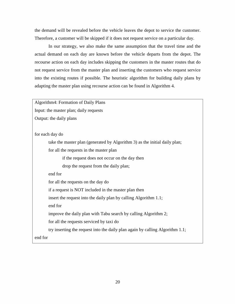
In our strategy, we also make the same assumption that the travel time and the
actual demand on each day are known before the vehicle departs from the depot. The
recourse action on each day includes skipping the customers in the master routes that do
not request service from the master plan and inserting the customers who request service
into the existing routes if possible. The heuristic algorithm for building daily plans by
adapting the master plan using recourse action can be found in Algorithm 4.
Algorithm4: Formation of Daily Plans
Input: the master plan; daily requests
Output: the daily plans
for each day do
take the master plan (generated by Algorithm 3) as the initial daily plan;
for all the requests in the master plan
if the request does not occur on the day then
drop the request from the daily plan;
end for
for all the requests on the day do
if a request is NOT included in the master plan then
insert the request into the daily plan by calling Algorithm 1.1;
end for
improve the daily plan with Tabu search by calling Algorithm 2;
for all the requests serviced by taxi do
try inserting the request into the daily plan again by calling Algorithm 1.1;
end for

21
5. Experimental Results
5.1 Results on Randomly Generated Data Sets
We first test our heuristic using simulation on randomly generated data sets.
Consider a city to be serviced with a two-dimensional coordinate system. The boundary
of the city is from -10 to 10 miles in both the x-axis and the y-axis. The depot and the
only lab where all the vehicles start and end their services every day are located at the
center of the city, that is (0, 0) on the two-dimensional plane.
The location of all the potential customers are known a priori, and the potential
customers, in each experiment, are uniformly distributed in the city. Some customers
request service at a fixed time every day (regular deterministic requests), while others
only request services at a fixed time on some of the days (urgent random requests). Each
random request has a probability of occurring on each day where is sampled from a
uniform [0, 1] distribution. The earliest pickup time (the earliest time a customer can be
visited) of a request is uniformly distributed from 9 am to 5 pm on each day. The latest
pickup time (the latest time a customer can be visited) of the request is 30 minutes after
the corresponding earliest pickup time. Each request has a latest drop-off time (a deadline
by which the sample has to be delivered to the lab); the latest drop-off time for regular
requests is 2 hours after its earliest pickup time, and the latest drop-off time for urgent
requests is 1 hour after its earliest pickup time (see Table 5.1). We assume all the
random requests are urgent requests. We also assume a given number of vehicles to
service the requests, which might be different in each experiment. And the vehicles drive
at an average speed of 30 miles per hour to service the requests.
Table 5.1: Time Windows of Regular and Urgent Requests
Earliest Pickup Time
(hours) Latest Pickup Time (hours) Latest Drop-off Time
(hours) Regular Request [9, 17] Uniformly 0.5+Earliest Pickup Time 2 + Earliest Pickup Time
Urgent Request [9, 17] Uniformly 0.5 + Earliest Pickup Time 1 + Earliest Pickup Time

22
We show the simulation results with the above assumptions and data inputs. In
each experiment, we assume a fixed number of potential requests, a fixed proportion of
deterministic requests among all the requests, and a fixed number of available vehicles to
handle the requests. The result of each experiment is taken by averaging the results of 10
replications, each of which takes the average result of 10 days. In each replication, a
random request customer is assigned a probability p of occurring, where p is a sample
from a uniform [0, 1]. In each day of a replication, we determine the occurrence of each
request by sampling based on the probability .
In each experiment, we compare the following four strategies by average travel
distance, average taxi cost, average route dissimilarity, average number of taxi trips,
average travel distance per requests, and average total cost, on a daily basis.
A. TAXI: schedule all the deterministic requests as master routes using the insertion
heuristic algorithm; use a third party courier, i.e., taxi, for all the random requests.
(Apply Algorithm 3 with a customer occurrence probability threshold of 1 to
build the master routes; handle all the random requests by taxi.)
B. IND: form a schedule independently for each day, using the insertion heuristic.
(Use Algorithm 1 to build daily routes independently.)
C. MFIX: schedule the deterministic requests as master routes, and insert the random
requests into the scheduled routes on each day. Use taxi if it is infeasible or more
expensive to insert the random request into the scheduled routes. (Use Algorithm
3 to build the daily plans with a customer occurrence probability threshold of 1.)
D. MHALF: schedule the deterministic requests and high occurring probability
requests (those who have an occurrence probability of 0.5 or higher) as master
routes. In the daily schedules, skip the non-occurring customers and insert the
unscheduled random requests into the scheduled routes. Use a taxi if it is
infeasible or more expensive to insert the random request into the scheduled
routes. (Use Algorithm 3 to build the daily plans with a customer occurrence
probability threshold of 0.5.)
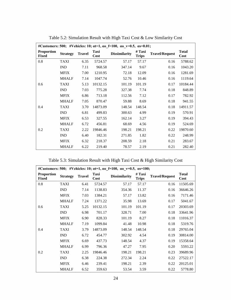
The parameters we use in the experiments for the Tabu search algorithms are
, , , , and . Table 5.2, Table 5.3,
and Table 5.4 summarize the simulation results with 500 customers, 10 vehicles and

23
different combinations of the cost parameters. In these tables, is the unit cost per hour
traveled. is the fixed cost per trip of taxi usage. is the variable cost per hour the
taxi traveled. is the unit cost per count of dissimilarity. Column “Proportion Fix”
shows the proportion of deterministic customers among all the potential customers.
Column “Strategy” lists the four compared strategies. Column “Travel” shows the total
distance that a vehicle travels per day on average. Column “Taxi Cost” shows the average
daily taxi cost. Column “Dissimilarity” shows the average dissimilarity, which is the total
number of vehicles used in the daily routes that is different than the one in the master
routes. If a taxi is used, then the dissimilarity is increased by one, as we assume that a
different taxi is used each time one is needed. Moreover, as there is no master routes
generated for independent scheduling, the dissimilarity is calculated by comparing the
daily routes to the master routes generated in strategy “master fix”. Column “#Taxi
Trips” shows the total number of daily taxi trips introduced on average. Column
“Travel/Requests” shows the distance that a vehicle travels to service a request on a daily
basis on average. Column “Total Cost” shows the average daily total cost including travel
cost, taxi cost, and cost on dissimilarity. It is the summation of each type of costs
weighted by the unit cost of that type.
24
Table 5.2: Simulation Result with High Taxi Cost & Low Similarity Cost
#Customers: 500; #Vehicles: 10; αt=1, αo_f=100, αo_v=0.5, αs=0.01;
Proportion
Fixed Strategy Travel
Taxi
Cost Dissimilarity
# Taxi
Trips Travel/Request
Total
Cost
0.8 TAXI 6.35 5724.57 57.17 57.17 0.16 5788.62
IND 7.11 968.58 347.14 9.67 0.16 1043.20
MFIX 7.00 1210.95 72.18 12.09 0.16 1281.69
MHALF 7.14 1047.74 52.76 10.46 0.16 1119.64
0.6 TAXI 5.13 10132.15 101.19 101.19 0.17 10184.44
IND 7.03 775.28 327.38 7.74 0.18 848.89
MFIX 6.86 713.18 112.56 7.12 0.17 782.92
MHALF 7.05 870.47 59.88 8.69 0.18 941.55
0.4 TAXI 3.70 14873.09 148.54 148.54 0.18 14911.57
IND 6.81 499.83 300.63 4.99 0.19 570.91
MFIX 6.53 327.55 162.14 3.27 0.19 394.43
MHALF 6.72 456.81 68.69 4.56 0.19 524.69
0.2 TAXI 2.22 19846.46 198.21 198.21 0.22 19870.60
IND 6.40 182.31 271.85 1.82 0.22 248.99
MFIX 6.32 218.37 208.59 2.18 0.21 283.67
MHALF 6.22 219.40 78.57 2.19 0.21 282.40
Table 5.3: Simulation Result with High Taxi Cost & High Similarity Cost
#Customers: 500; #Vehicles: 10; αt=1, αo_f=100, αo_v=0.5, αs=100;
Proportion
Fixed Strategy Travel
Taxi
Cost Dissimilarity
# Taxi
Trips Travel/Request
Total
Cost
0.8 TAXI 6.41 5724.57 57.17 57.17 0.16 11505.69
IND 7.14 1138.83 354.36 11.37 0.16 36646.26
MFIX 7.03 1384.21 57.17 13.82 0.16 7171.46
MHALF 7.24 1371.22 35.98 13.69 0.17 5041.67
0.6 TAXI 5.25 10132.15 101.19 101.19 0.17 20303.69
IND 6.98 701.17 328.71 7.00 0.18 33641.96
MFIX 6.90 828.33 101.19 8.27 0.18 11016.37
MHALF 7.19 1099.84 41.48 10.98 0.18 5319.76
0.4 TAXI 3.79 14873.09 148.54 148.54 0.18 29765.04
IND 6.72 454.77 302.92 4.54 0.19 30814.00
MFIX 6.69 437.73 148.54 4.37 0.19 15358.64
MHALF 6.99 796.36 47.27 7.95 0.20 5593.22
0.2 TAXI 2.25 19846.46 198.21 198.21 0.23 39689.96
IND 6.38 224.38 272.34 2.24 0.22 27522.17
MFIX 6.46 239.41 198.21 2.39 0.22 20125.01
MHALF 6.52 359.63 53.54 3.59 0.22 5778.80

25
Table 5.4: Simulation Result with Low Taxi Cost & High Similarity Cost
#Customers: 500; #Vehicles: 10; αt=1, αo_f=0.5, αo_v=0.5, αs=100;
Proportion
Fixed Strategy Travel
Taxi
Cost Dissimilarity
# Taxi
Trips Travel/Request
Total
Cost
0.8 TAXI 6.26 36.16 57.17 57.17 0.16 5815.79
IND 6.73 12.99 353.80 19.03 0.16 35460.30
MFIX 6.87 9.45 57.17 14.19 0.16 5795.20
MHALF 7.28 9.17 35.98 13.88 0.17 3679.95
0.6 TAXI 5.14 63.74 101.19 101.19 0.17 10234.18
IND 6.46 12.53 328.73 18.27 0.17 32950.16
MFIX 6.76 8.77 101.19 13.03 0.17 10195.34
MHALF 7.16 7.91 41.48 11.88 0.18 4227.55
0.4 TAXI 3.73 93.37 148.54 148.54 0.18 14984.68
IND 6.15 11.64 301.84 16.97 0.18 30257.15
MFIX 6.33 8.88 148.54 13.03 0.19 14926.16
MHALF 6.92 5.71 47.27 8.50 0.20 4801.94
0.2 TAXI 2.21 124.57 198.21 198.21 0.22 19967.66
IND 5.65 11.87 271.81 17.30 0.20 27249.35
MFIX 5.82 10.35 198.21 15.09 0.21 19889.57
MHALF 6.39 3.19 53.54 4.67 0.22 5421.10
From the simulation results, we make the following observations:
I. Strategy TAXI has the smallest travel distance and largest taxi cost, because
of its inability to use the slack times to accommodate the random requests,
thus resulting in servicing fewer requests by the regular fleet. Strategy MFIX
and MHALF have similar “travel distance per request” as strategy IND, a
near-optimal routing solution, suggesting that our master plan strategies
provide efficient routing solutions.
II. Strategy IND has the largest dissimilarity; strategy MHALF has the lowest
dissimilarity. If we schedule the routing for each day independently without a
master plan, the routes become dissimilar from day to day. Even though we
get an efficient route as measured in travel distance and taxi cost, the quality
of service, as measured in route dissimilarity, is poor. If we form master
routes with the deterministic requests and a number of random requests of

26
high probability of occurrence, daily routes are created, which are similar
from day to day, without scarifying much in routing efficiency.
III. When the unit cost for route dissimilarity increases (from 0.01 to 100), the
dissimilarity for strategies with master plans decreases and the routing
efficiency (travel distance and taxi cost) increases. This is because when we
give a higher weight on dissimilarity, the routing solution favors less
dissimilarity, and trades that with less routing efficiency. The change in the
unit cost for route dissimilarity does not significantly impact the solutions of
strategies TAXI and IND. The reason is that for strategy TAXI, the
dissimilarity is contributed by the random requests handled by taxi, which
remain the same with any set of parameters; for strategy IND, there is no
master plan to use to construct daily routes, but the dissimilarity is measured
against the master plan from strategy MFIX. Hence, the dissimilarity with
IND might even increase when the unit cost of dissimilarity increases.
IV. When the fixed unit taxi cost decreases (from 100 to 0.5), while all the other
parameters remain the same, there is more taxi use represented by the
number of taxi trips. This implies that as taxi usage become inexpensive, it
becomes a more economical solution to use taxi rather than rerouting to pick
up packages by the regular fleet of vehicles.
5.2 Results with Actual Data
We tested our routing approach also using real-life data collected from a leading
healthcare provider in Southern California. There are two types of requests in the data set.
One is regular daily requests, which needs to be visited every day at a specific time. The
other is random requests that are currently being outsourced to a taxi service. We have
compared three strategies with this set of data.
1) MD Routes: Include a customer into the master plan if the pickup and delivery
location of a request has a probability of occurring higher than a threshold
(e.g., 10%). Recourse for daily plans.
2) Industry Reroute: Take the existing master plan from the healthcare provider
as the simulated master routes. Recourse for daily plans.

27
3) Industry Taxi: Take the existing master plan from the healthcare provider as
the daily routes. Use Taxi for all the random requests.
In the above strategies, the recourse action means dropping the non-occurring
requests and inserting the occurring requests on a daily basis. It should be noted that
Industry Taxi is the current practice of this healthcare provider. In the following
simulation with 30 scenario days, there are 85 deterministic requests and 100 potential
random requests on each day and the occurrence probability on each day for these
random requests vary from 0 to 0.20. These requests are scattered across 16 medical
centers and the pickup and delivery of the requests can be at any of these centers. The
time windows are 4 hours for regular requests and 2 hours for urgent requests. On a daily
basis, 14 regular fleet vehicles are available to service the requests.
The simulation results are shown in
Table 5.5, and we see that strategy “Industry Taxi” has the shortest average travel
time. The table also shows that the taxi cost and the number of taxi trips of strategy
“Industry Taxi” are significantly higher than those of the strategies with recourse actions
(MD Routes and Industry Reroute). This implies that, with the recourse technique, we are
able to better utilize the slack time on the vehicles to reduce the taxi cost. Meanwhile,
even though the average total travel time of a vehicle is higher with the strategies with
recourse actions, the average travel time spent for each customer request is lower with
these strategies. From the table, we also see that the proposed strategy – MD Routes has
the smallest taxi cost and average travel time per request. This shows that the proposed
strategy not only better utilizes the slack time to reduce the taxi cost, but is also an
efficient routing solution with the least travel time spent on each request.
Besides the reduction in taxi cost, MD Routes significantly reduced the route
dissimilarity. In general, any strategy with a rerouting technique has smaller dissimilarity
as the location visited in the master plan is going to be more frequently repeated in the
daily plans. And the strategy we propose is the best in generating similar routes. This is
achieved by having the proposed strategy “MD Routes” including the high probabilistic
customers into the master routes; whereas the strategy “Industry Reroute” has only the
deterministic customers in the master plan.

28
The results of the analysis with real-life data shows that our heuristic can improve
the routing solution by decreasing the taxi and dissimilarity costs. With the current
resource of vehicles, the current deterministic requests, and sampling on current data set,
our heuristic beats the current industry solution by reducing the taxi cost by 45%-48%and
reducing dissimilarity by 26%-33%. If we compare with the daily routes obtained by
applying the recourse actions on a master plan taken from the current industry practice,
our heuristic reduces the taxi cost by 16%-17% and it reduces dissimilarity by 9%-12%.
Table 5.5: Simulation Results with Actual Data
αt=1, αo_f=100, αo_v=0.5, αs=0.01;
Strategy Travel
(hours/day)
Taxi Cost
($/day)
Dissimilarity
(counts/day)
# Taxi Trips
(trips/day)
Travel/Request
(hours/day)
Total Cost
($/day)
MD Routes 8.78 5221.10 148.00 52.10 0.03 5345.50
Industry Reroute 8.36 6223.40 164.00 62.10 0.03 6342.10
Industry Taxi 7.24 10023.80 200.00 100.00 0.04 10127.20
αt=1, αo_f=100, αo_v=0.5, αs=100;
Strategy Travel
(hours/day)
Taxi Cost
($/day)
Dissimilarity
(counts/day)
# Taxi Trips
(trips/day)
Travel/Request
(hours/day)
Total Cost
($/day)
MD Routes 8.82 5291.13 143.40 52.77 0.03 19754.60
Industry Reroute 8.47 6333.60 157.23 63.17 0.03 22175.51
Industry Taxi 7.24 10023.77 200.00 100.00 0.04 30125.17
αt=1, αo_f=0.5, αo_v=0.5, αs=100;
Strategy Travel
(hours/day)
Taxi Cost
($/day)
Dissimilarity
(counts/day)
# Taxi Trips
(trips/day)
Travel/Request
(hours/day)
Total Cost
($/day)
MD Routes 8.13 43.60 134.23 54.57 0.03 13580.76
Industry Reroute 8.08 49.79 152.93 64.20 0.03 15456.24
Industry Taxi 7.24 73.77 200.00 100.00 0.04 20175.17
6. Conclusions
In this study, we consider a Courier Delivery Problem (CDP), a variant of the
Multi-trip Vehicle Routing Problem (MVRP) with uncertainty in customer occurrence
and urgency in customer demands. We present a problem formulation with mixed integer
programming for an example application of the transportation of medical specimens. We
develop an efficient heuristic based on insertion and tabu search. Our model represents
the probabilistic nature of customer occurrence using scenario-based stochastic

29
programming with recourse. We benefit from the simplicity and flexibility of a master
plan with daily recourse actions.
Our model first includes a master plan problem which represents the uncertainty
in the customer occurrence by the probabilities customers are likely to appear and
addresses the urgency in delivery time windows by use of the fleet of vehicles in multiple
trips. We then define a recourse action of partial rescheduling of routes by omitting non-
occurring customers and rescheduling new customers. The master routes created consider
efficiency in routing, to represent slack time for accommodating random requests. The
daily plans created take into account the efficiency in routing, efficiency in alternative
third party courier, as well as route similarities to boost the quality of service. To solve
large size problems of the model, we develop a heuristic based on insertion and tabu
search.
We explore experimentally the sensitivity of our heuristic on randomly generated
problems and a real-life problem collected from industry. Experiments on randomly
generated problems include sensitivity analysis in varying problem size, customer
uncertainty scenarios, resource availability and cost parameters. We compare the quality
of the solution with independent daily scheduling, and to an industry standard solution. In
the experiments with real-life data, we compare the quality of the solution with the
current industry solution with and without recourse action. Sensitivity analysis on varying
cost parameters shows that our heuristic produces a better solution than the current
practice by significantly reducing the cost on taxi use and improving route similarity.

30
References
Alonso F., Alvarez M.J., and Beasley J.E., “A tabu search algorithm for the periodic
vehicle routing problem with multiple vehicle trips and accessibility restrictions,”
Journal of the Operational Research Society, 59, 963-976, 2008.
Angelelli E. and Speranza M.G., “The periodic vehicle routing problem with intermediate
Facilities,” European Journal of Operational Research, 137, 233-247, 2002.
Astion ML, Shojania KG, Hamill TR, Kim S, and Ng V.L., “Classifying laboratory
incident reports to identify problems that jeopardize patient safety,” Am J ClinPathol,
120, 18-26, 2003.
Azi N., Gendreau M., and Potvin J., “An exact algorithm for a single-vehicle routing
problemwith time windows and multiple routes,” European Journal of Operational
Research, 178,755–766, 2006.
Bertsimas D., Jaillet P., and Odoni A.R., “A-priori optimization,” Operations Research,
38, 1019-1033, 1990.
Bertsimas D., “A vehicle routing problem with stochastic demand,” Operations
Research, 40, 574-585, 1992.
Bertsimas D. and Simchi-leviD., “A new generation of vehicle routing research: robust
algorithms, addressing uncertainty,” Operations Research, 44, 2, 286–304, 1996.
Brandao J. and Mercer A., “A tabu search algorithm for the multi-trip vehicle routing and
scheduling problem,” European Journal of Operational Research, 100, 180–191, 1997.
Brandao J. and Mercer A., “The multi-trip vehicle routing problem,” The Journal of the
Operational Research Society, 49, 799-805, 1998.

31
Campbell A. M. and Savelsbergh S., “Efficient insertion heuristics for vehicle routing
and scheduling problems,” Transportation Science, 38, 3, 369-378,2004.
Francis P. and Smilowitz K., “Modeling techniques for periodic vehicle routing
problems,” Transportation Research Part B: Methodological, 40, 872-884, 2006.
Gendreau M., Laporte G., and Seguin R., “An exact algorithm for the vehicle routing
problem with stochastic demands and customers,” Transportation Science, 29, 143-155,
1995.
Gendreau M., Laporte G., and Seguin R., “Stochastic vehicle routing,” European
Journal of Operational Research, 88, 3-12, 1996.
Groër C., Golden B., and Wasil E., “The consistent vehicle routing problem,”
Manufacturing and Service Operations Management, 11, 630-643, 2009.
Haughton M., “Quantifying the benefits of route reoptimization under stochastic
customer demands,” Journal of the Operational Research Society, 51, 320–322, 2000.
Haughton M. and Stenger A., “Modeling the customer service performance of fixed
routes delivery systems under stochastic demands,” Journal of Business Logistics, 9,
155–172, 1998.
Hemmelmayr, V.C., Doerner, K.F., and Hartl, R.F., “A variable neighborhood search
heuristic forperiodic routing problems,” European Journal of Operational Research,
195, 791-802, 2009.
Ichoua S., Gendreau M., and Potvin J., “Exploiting knowledge about future demands for
real-time vehicle dispatching,” Transportation Science, 40, 211-225, 2006.

32
Kellerer.H., U. Pferschy, and D.Pisinger, Knapsack Problems, SpringerVerlag Berlin
Heidelberg, 2004.
Laporte G., Louveaux F.V., and Mercure H., “A priori optimization of the probabilistic
traveling salesman problem,” Operations Research, 42, 543-549, 1994.
Lin S., “Computer solutions of the traveling salesman problem,” Bell System Technical
Journal, 44, 2245-2269, 1965.
Osman I.H., “Metastrategy simulated annealing and tabu search algorithms for the
vehicle routingproblem,” Annals of Operations Research, 41, 421-451, 1993.
Petch R. J. and Salhi S., “A multi-phase constructive heuristic for the vehicle routing
problemwith multiple trips,” Discrete Applied Mathematics, 133, 69-92, 2003.
Ren Y., Dessouky M. M., and OrdonezF., “The multi-shift vehicle routing problem with
overtime,” Computers & Operations Research, 37, 1987-1998, 2010.
Salhi S. and Petch R. J., “A GA based heurisric for the vehicle routing problem with
multiple trips,” Journal of Mathematical Modeling and Algorithms, 6, 591—613, 2007.
Secomandi N.,“A rollout policy for the vehicle routing problem with stochastic
demands,”Operations Research, 49, 796 - 802, 2001.
Spivey M. and Powell W.B., “The dynamic assignment problem,” Transportation
Science, 38, 399 - 419, 2004.
Sungur I., Ordonez F., Dessouky M. M., RenY., and ZhongH., “A model and algorithm
for the courier delivery problem with uncertainty,” Transportation Science, 44, 193-205,
2010.

33
Taillard E., Laporte G., and Gendreau M., “Vehicle routing with multiple use of
vehicles,” Journal of the Operational Research Society, 47, 1065–1070, 1996.
Yang W. H., Mathur K., and Ballou R. H., “Stochastic vehicle routing problems with
restocking,” Transportation Science, 34, 99-112, 2000.
Zapfel G., and Bogla M., “Multi-period vehicle routing and crew scheduling with
outsourcingoptions,”International Journal of Production Economics,113, 980-996, 2008.
Zhong, H., Hall R. W., and Dessouky M. M., “Territory planning and vehicle
dispatching,” Transportation Science, 41, 74-89, 2007.


![TDRS–Transportation, Delivery and Relocation SolutionsLocal Courier Delivery Services, SIN 451-3 (Small Business Set Aside [SBSA]) Local courier delivery services are available for](https://cdn.vdocuments.site/doc/165x107/60154f8ca720bf5ec51f344d/tdrsatransportation-delivery-and-relocation-solutions-local-courier-delivery.jpg)