
ARTICLE IN PRESS
0889-9746/$ - se
doi:10.1016/j.jfl
�CorrespondE-mail addr
X.Y.Luo@shef
Journal of Fluids and Structures 20 (2005) 129–140
www.elsevier.com/locate/jfs
Blood flow and damage by the roller pumps duringcardiopulmonary bypass
J.W. Mulhollanda,b, J.C. Sheltonb, X.Y. Luoc,�
aLondon Perfusion Science, Clinical Perfusion, London Independent Hospital, 1 Beaumont Square, Stepney Green, London E1 4NL, UKbDepartment of Engineering, Medical Engineering Division, Queen Mary, University of London, London E1 4NS, UK
cDepartment of Mechanical Engineering, University of Sheffield, Mappin Street, Sheffield S1 3JD, UK
Received 8 October 2002; accepted 6 October 2004
Abstract
Although much CFD work has been carried out to study the blood damage created in a centrifugal pump used for a
cardiopulmonary bypass, little is known about the blood flow and consequent damage in a roller pump. A time-
dependent moving boundary problem is solved in this paper to explore the blood flow and damage in the roller pump.
An initial attempt to predict the blood damage from these simulations is also made and results are compared with
experimental observations. It is discovered that reducing the amount of time two rollers simultaneously occlude the
tubing, will reduce the blood exposure to shear stress significantly and consequently reduce the blood damage caused.
r 2004 Elsevier Ltd. All rights reserved.
1. Introduction
During open-heart surgery, cardiopulmonary bypass (CPB) is used to isolate the heart and lungs from the remainder
of the circulation. The primary function of the heart and lungs is the provision of blood circulation, to provide oxygen
and other nutrients to the cells and to remove the products of metabolism. These functions are therefore undertaken by
the CPB system. The blood gas exchange device (oxygenator) performs the function of the lung by adding oxygen to the
blood whilst carbon dioxide is removed. During CPB the venous return to the right heart is diverted via a cannula by
syphonage to the venous reservoir of the CPB system. The venous reservoir has two roles. It acts as a capacitance
chamber, which allows for variations in the patient’s circulating volume, and it also filters the blood removing air and
other embolic material. A roller, or centrifugal pump, the analogue of the left ventricle, sucks blood from the reservoir
and pumps it through the heat exchanger and the oxygenator. Blood that spills into the open chest cavity is returned to
the systemic system via a low-pressure suction system which is driven by a separate roller pump.
It is well established that CPB damages the blood (Mulholland et al., 2000; Yarbourgh et al., 1966) by subjecting it to
non-physiological forces (Blackshear et al., 1965; Nevaril et al., 1968; Leverette et al., 1972; Williams, 1973; Bernstein et
al., 1967; Bluestein and Mockros, 1969), therefore prolonging the patient’s recovery. A great deal of research has been
focused on reducing this damage. Many major advances in CPB have been achieved, for example oxygenators are more
efficient, the materials used are more biocompatible and the circuits are therefore safer. Nevertheless, it has become
e front matter r 2004 Elsevier Ltd. All rights reserved.
uidstructs.2004.10.008
ing author. Tel.: +44114 2227752; fax: +44 114 2227890.
esses: [email protected] (J.W. Mulholland), [email protected] (J.C. Shelton),
field.ac.uk (X.Y. Luo).

ARTICLE IN PRESSJ.W. Mulholland et al. / Journal of Fluids and Structures 20 (2005) 129–140130
important to reconsider some of the more detailed aspects of the current system in terms of the precise nature of the
damage to the blood cells. Improving the way blood flows through the circuit is a key area for the advancement of CPB.
The geometry of the circuit will influence the fluid dynamics in the system and therefore how the blood is handled.
Detrimental flow structures such as areas of turbulence, stagnation, vortices, recirculation, high shear stresses, and
negative pressure all contribute to increased blood damage (Mulholland et al., 2000).
One of the key areas of the CPB circuit is the arterial pump, which provides the blood with momentum. There are
two types of pump currently used, the roller pump (peristaltic) and the centrifugal pump (constrained vortex). It was
believed when the centrifugal pump was introduced into the CPB circuit, as the arterial pump, that their evolution
would eventually render the roller pump obsolete. With recent independent research failing to show any advantage of
using a centrifugal pump over a roller pump (Hansbro et al., 1999; Takahama et al., 1985) for short-term assist (less
than 8 h), perfusionists continue to use roller pumps as the arterial pump as they are simple and cost effective. The
initial expectations of the centrifugal pump led to a considerable amount of numerical simulation (Anderson et al.,
2000; Bludszuweit, 1995a; Sukumar et al., 1996; Nakamura et al., 1999; Huang and Fabisiak, 1978; Miyazoe et al.,
1998, 1999; Takiura et al., 1998) being carried out on this device. There has been little published literature investigating
the roller pump during the past 20 years. This paper presents a two-dimensional numerical simulation of a roller pump.
The aims were to understand the detailed fluid dynamics of the roller pump and assess the potential of using the CFD
results in a theoretical blood damage prediction model. In order to accurately understand blood flow in a roller pump it
was necessary to perform a time-dependent flow simulation with a deforming mesh. The detailed flow patterns, as well
as shear stress in the flow were examined. Although this is a two dimensional approach, it provides the first step towards
a more realistic model. These results will be used to identify the deficiencies of the current designs for roller pumps from
a fluid dynamic point of view. The hypothesis was set that if an accurate model of the roller pump could be generated
using CFD it would be possible to refine the design more easily and thereby reduce the amount of blood damage caused.
2. The model
2.1. The geometry
A two-dimensional model of the system was obtained using an established protocol that combined computer-aided
drawings, a digital camera and digitization of these images (Fig. 1). The digital camera was positioned over the central
point of the roller pump using a plumb line and a spirit level. The silicon roller pump boot is shown in Fig. 1. It lies
along the wall of the pump housing, and is compressed by the rollers providing peristaltic flow. Images of the roller
pump boot were taken at every degree between y ¼ 01 and 1801 in order to establish the changes in geometry. The pump
boot was filled with black dye making the inner edges clearly definable.
Occlusion of the roller pump, i.e. the distance between the inner walls of the pump boot at the point of roller contact
was set to be just under occlusive using a qualitative, clinically established protocol (London Independent Clinical
Protocols, 1994). The rollers are manually tightened to be fully occlusive using the pumps integrated control. The outlet
of the pump boot is clamped off and the roller is turned to generate a positive pressure of 280mmHg ensuring the
leading roller is positioned at y ¼ 901: The pressure is measured at the outlet of the pump boot using a Tycos pressure
gauge that is an integrated part of the CPB tubing circuit. The roller occlusion is then loosened until the pressure
decreases at a rate of 1mmHg/s. Using the same method the occlusion of both rollers are checked with the leading roller
at y ¼ 01; 451 and 1351. The protocol has been designed to minimize the back-flow caused by significant under-
occlusion whilst avoiding cell crushing caused by over-occlusion. The geometry acquisition technique showed that with
the occlusion set correctly, the gap between the inner walls at the point of roller contact was 1mm.
2.2. Governing equations
The Navier–Stokes equations are given below, where r is the fluid density, ui is the velocity component in the xi
direction (i ¼ 1; 2), p is the pressure, tij is the stress tensor, and repeated indices are summed:
@ui
@xi
¼ 0; (1)
r@ui
@t
� �þ
@
@xj
uiuj
� �� �¼ �
@p
@xi
þ@tij
@xj
: (2)
These are solved using a commercial CFD package Fluent 4.

ARTICLE IN PRESS
2
x
x1
y
x
θ - Start Point = 0º
θω
CentralPoint
Inner Wall (Iw)Start Point
Fixed Wall uw = vw = o
Silicon RollerPump Boot
Trailing Roller
Inner Wall (Iw) - Moving Boundary
Leading Roller
Individual Mesh Cell
Outlet(Zero Normal Gradient)
Channel Width (H) Inlet uinlet = 0.35 m/s
Qinlet = 2.47x10⁻³ m3/s
Fig. 1. The geometry, boundary conditions and meshing of the roller pump boot.
J.W. Mulholland et al. / Journal of Fluids and Structures 20 (2005) 129–140 131
Blood was modelled as Newtonian, with a constant density of 1050 kg/m3 and a constant viscosity of 3.5� 10�3 kg/
m s. The Casson plot (Fung, 1993) showed that blood demonstrates non-Newtonian properties at low shear rates (less
than 100 s�1), whilst above this threshold shear rate blood exhibits Newtonian properties. These findings were
confirmed by Huang and Fabisiak (1978), and Bludszuweit (1995a), who both showed that at higher shear rates blood
can be modelled as Newtonian. This assumption of Newtonian behaviour holds for the shear rates found in this
simulation.
2.3. Initial and boundary conditions
2.3.1. Initial conditions
As the initial conditions are themselves a solution of the system at the end of each cycle, one of the early simulations
was run for five revolutions. It was found that the results stabilized and began repeating every 1801 after 5401
(112revolutions). The results data file at y ¼ 5401 was used to supply the initial conditions for the final case file.
2.3.2. Boundary conditions
The boundaries of the model consisted of an inlet, an outlet, a no-slip wall boundary, and a moving boundary (see
Fig. 1). The flow rate was measured to be 2.47� 10�5m3/s, which corresponded to an inlet velocity of 0.35m/s, giving a
Reynolds number Re ¼ ruinletH=m ¼ 496: A parabolic velocity profile was used at the inlet, and zero pressure was
specified at the outlet. The velocity at the stationary and moving walls of the pump boot satisfied the no-slip condition.

ARTICLE IN PRESSJ.W. Mulholland et al. / Journal of Fluids and Structures 20 (2005) 129–140132
3. Methods
The simulation was time dependent and the shape of the pump boot changed with time. This shape is associated with
the periodic passage of the rollers.
3.1. The time-dependent model
To solve this time-dependent moving boundary problem, the model was set to automatically save the data files every
5 time steps (0.51). The time-dependent and deforming mesh models were used at each time step to describe the grid
deformation with interpolation between files. The time-dependent equations were solved using an implicit formulation,
requiring iteration at each time step, and the maximum number of iterations per time step was set to 100. The minimum
residual sum was set to 10�3. Convergence was achieved when the sum of the absolute values of normalized residuals
was less than this value. The number of time steps between each grid file was set to 10, thereby determining the size of
the time step Dt as 3.44� 10�4 s, which was the time taken for the roller to travel 0.11.
3.2. The computational methods and the deforming mesh model
At each time step, the model was solved using a power law discretization scheme, which provides a formal accuracy
between 1st and 2nd order schemes. The components of the velocity were updated used a line Gauss–Seidel equation
solver, which was set to sweep in a direction normal to the primary direction of flow. In order to speed the convergence
of the standard line solver, a multigrid scheme was used to solve the pressure correction equations.
As the grid topology must not change throughout the calculation, it was important that the deformation of the mesh
should not proceed to the extent that a skewed mesh was generated. This would produce inaccurate results and was
therefore carefully considered during the initial mesh generation.
A summary of the method used to generate the CFD model of the roller pump is shown in Fig. 2. A geometry file was
created for each degree throughout the rotation. The size and topology of the mesh was determined from a single
geometry file.
4. Code validation
Finding the optimum grid size and the optimum time step were important to ensure that accurate results were
obtained using the minimum amount of computer memory and time. The method that was used to determine these
values involved changing the size of each parameter in turn. The size of the mesh was increased while the time step was
reduced. The model was initially meshed (2136 cells—angular interval ¼ 0.811) and modeled under the steady state
condition when two rollers are in the position of y ¼ 0: The mesh size was increased to 6886 cells (angular
interval ¼ 0.421) and the analysis carried out again. This process was repeated until the difference in maximum vorticity
between the two sets of results was less than 1%. The mesh at this point had 21,639 cells (angular interval ¼ 0.261), and
was taken to be the optimum grid size.
This mesh was then incorporated into a time-dependent case file along with the boundary conditions and the
deforming mesh model. The model was initially run with a 1.13� 10�3 s (11) time step; the time step was then reduced to
5.67� 10�4 s (0.51). This process was also repeated until the difference in maximum vorticity between the two sets of
results was less than 1%. The optimal time step was found to be 3.44� 10�4 s (0.31).
5. Results
5.1. Velocity fields
Due to the large amount of data produced in this time-dependent simulation, only velocity magnitude contours are
shown for selected parts of the flow domain at selected times. However, the observations we made also included flow
information not shown here.
The velocity magnitude contours of the flow near the rollers at various roller positions from y ¼ 01 to 1801 are shown
in Figs. 3(a)–(e). The scales are not the same for each figure, as this would result in poor velocity contour distinction in
individual plots. At y ¼ 01; both the leading roller (grey) and the trailing roller (white) are occluding the tube. The
maximum velocity occurs at the narrowest part of the tube and is as high as 11.31m/s, since the gap between the roller

ARTIC
LEIN
PRES
S
Digital Camera
Acquire Geometry
Create Geometry File for One
DegreeCreate Mesh File
Set BoundaryConditions
Run Steady StateComputation(Iterate) for 1
Degree
Data ThiefSoftware
More Accurate(> 1%)
Divergence Convergence
Increase Size of Mesh File
Run Steady State Computation (Iterate) for 1
Degree
Assess Accuracy of Results (< or >
1% difference from smaller file)
No Significant Increase in
Accuracy of Results (< 1%)
Optimum MeshSize
Create Geometry File for Every
Degree
Create Mesh Filefor Every Degree
Create Case File for Time
DependentModel
RunComputation ofTime Dependent
Model
Decrease Size of Time Step
Run Computation of Time Dependent
Model
Assess Accuracyof Results (< or >
1% difference from larger step)
More Accurate(> 1%)
No SignificantIncrease in
Accuracy of Results (< 1%)
AnalyseResults
Create Case Filefor Time
DependentModel
Optimum TimeStep
Fig. 2. Flow diagram illustrating method used to create the CFD model of roller pump.
J.W
.M
ulh
olla
nd
eta
l./
Jo
urn
al
of
Flu
ids
an
dS
tructu
res2
0(
20
05
)1
29
–1
40
133

ARTICLE IN PRESS
θ = 0º Leading Roller
(a)
θ = 0º Trailing Roller
θ = 30º Leading Roller
(b)
θ = 45º Leading Roller
(c)
θ = 90º Leading Roller
(d)
θ = 90º Trailing Roller
θ = 45º Trailing Roller
θ = 30º Trailing Roller
θ = 165º Leading Roller
(e)
θ = 165º Trailing Roller
Fig. 3. (a) Velocity magnitude contours plotted between 0 and 11.31m/s (maximum velocity) of the flow field near the rollers when
y ¼ 01. On the left is the flow near the leading roller and on the right is the flow near the trailing roller. (b) Velocity magnitude contours
of the flow field near the rollers when y ¼ 301, plotted between 0 and the maximum velocity of 0.87m/s. On the left is the flow near the
leading roller and on the right is the flow near the trailing roller. (c) Velocity magnitude contours of the flow field near the rollers when
y ¼ 451, plotted between zero and the maximum velocity of 0.63m/s. On the left is the flow near the leading roller and on the right is
the flow near the trailing roller. (d) Velocity magnitude contours of the flow field near the rollers when y ¼ 901, plotted between zero
and the maximum velocity of 0.60m/s. (e) Velocity magnitude contours of the flow field near the rollers when y ¼ 1651, plotted
between zero and the maximum velocity of 11.31m/s. On the left is the flow near the leading roller and on the right is the flow near the
trailing roller.
J.W. Mulholland et al. / Journal of Fluids and Structures 20 (2005) 129–140134

ARTICLE IN PRESSJ.W. Mulholland et al. / Journal of Fluids and Structures 20 (2005) 129–140 135
and the wall is very small ( ¼ 1mm). Flow separation regions are also observed downstream of both rollers. This is the
most dangerous position, which generates the maximum pressure drop, or resistance of the whole cycle. Then at
y ¼ 301; the leading roller is moving away from the wall, the flow is recovering near the leading roller, while a small flow
separation region still exists just downstream of the trailing roller. The maximum velocity drops to 0.87m/s. As the
rollers continue to move to y ¼ 451; the leading roller becomes detached from the wall, while the trailing roller is still
squeezing the tube. The flow separation zone disappears, and the maximum velocity further decreases to 0.63m/s. Then
at y ¼ 901; the rollers turn into a vertical position. The flow far away from the roller almost recovers to its undisturbed
Poiseuille flow state, with a maximum velocity of 0.60m/s. This is still much higher than the inlet velocity of 0.35m/s.
Finally, as the rollers move into position y ¼ 1651; both rollers start to squeeze the wall again, and the maximum
velocity near the leading roller increases sharply back to 11.31m/s. A large zone of flow separation is re-established
downstream of the leading roller, and then the whole pattern then starts to repeat itself from y ¼ 1801 (i.e. y ¼ 01)
again. Note that the trailing roller becomes the leading one as it passes through 901.
5.2. Wall shear stress
Fig. 4 shows the variation of the shear stress along the inner wall of the pump boot with varying roller position, y(1441–2161). As for the velocity magnitude, the peak value of the shear stress is seen with the leading roller in the
horizontal position, y ¼ 01 (i.e. y ¼ 1801).
A plot of peak shear stress along the whole length of the inner and outer walls for one full rotation is shown in Fig. 5.
The peak shear stress is defined as the maximum shear stress at any point along the length of the tube for that particular
time step (Dt). The plot shown starts at y ¼ 901 and ends at 2701 (half rotation). As the two rollers have identical
shapes, the pattern repeats itself after 1801. The results show that the blood experienced nearly 8% higher shear stresses
at the inner wall (994N/m2) compared to the outer wall (923N/m2) and therefore the remainder of the paper presents
the inner wall stresses (inner 994N/m2, outer 923N/m2). The significant shear stresses occur from y ¼ 1441 to 2161; asmarked on the graph. It is noted that a sharp peak of shear stress occurs at y ¼ 1801: This is the position when both
rollers are almost occluding the tube. There is a decrease in the volume of the tube as the second roller makes contact.
Because the fluid is incompressible, the pressure between the rollers becomes very high and the fluid is driven through
the narrow gaps very fast (as shown in Fig. 3). As a result, there exists a very thin boundary layer with high-velocity
gradient, thus giving rise to a sharp peak of shear stress.
In fact, the computed peak shear stress is limited by the numerical resolution near the boundary layer; the actual
value experienced by the blood cells may be even higher in this region.
y
x
1200
1000
800
600
400
200
0
0 0.05 0.1 0.15 0.2 0.25 0.3 0.35 0.4 0.45 0.5 0.55 0.6 0.65 0.7 0.75
Sh
ear
Str
ess
(N/m
2 )
Length Along Inner Wall (m)
Leading Roller Trailing Roller
θ = 180º
θ = 180º
θ = 144º
θ = 180º
θ = 216º
Fig. 4. Wall shear stress distribution along the arc length of the inner wall: five distributions are plotted at every 12 degrees from
y ¼ 1441 to 2161.

ARTICLE IN PRESS
0
100
200
300
400
500
600
700
800
900
1000
1100
90 100 110 120 130 140 150 160 170 180 190 200 210 220 230 240 250 260 270
Horizontal Roller Position (θ) - 0º
144 Horizontal 216
Sh
ear
Str
ess
(N/m
2 )
Roller Position – θ (degrees)
INNER
OUTER
Fig. 5. The peak wall shear stress tw distributed along the inner (solid) and outer (dashed) walls during a half rotation.
J.W. Mulholland et al. / Journal of Fluids and Structures 20 (2005) 129–140136
6. Discussion
Cardiopulmonary bypass technology has not benefited from a large amount of CFD research because most of the
current equipment was designed before CFD became widely available. Most of the CFD modelling carried out in the
CPB field has focused on the centrifugal pump. Miyazoe et al. (1998, 1999), concluded that CFD could be a useful tool
for developing blood pumps, but no direct comparisons between hemolysis tests and visualization tests were actually
performed. Work reported by Pinotti and Rosa (1995), Nishida et al. (1999) and Takiura et al. (1998), focused on
centrifugal pumps. Takiura et al. (1998) compared a selection of their CFD results with hemolysis tests and concluded
that they were consistent. Although it is hard to draw comparisons, all the researchers found CFD to be valuable tool
for developing blood pumps. This is one of the main aims of carrying out CFD analysis of the roller pump.
6.1. Wall shear stress
Blood experiences higher shear stresses at the inner wall than at the outer wall. This is because the velocity profile is
more skewed towards the inner wall due to centrifugal force, and gives rise to a higher gradient. Two regions were
observed during each rotation where increased shear stresses were predicted. The first occurred between y ¼ 1441 and
2161 at either side of the horizontal roller position (y ¼ 1801). The second occurs at the either side of y ¼ 01:In order to understand the mechanism causing the high shear stresses several parameters were considered. These
parameters have been plotted in Fig. 6. The peak shear stress, the occlusion of the leading roller, the average blood flow
velocity at the outlet boundary of the model, the occlusion of the trailing roller, and the pressure drop across the pump
boot were all plotted against roller position (y ¼ 144122161). The outlet flow velocity generated by the pump is actually
pulsatile, varying from 0.71m/s at y ¼ 1681 to 0.10m/s at y ¼ 2021: This is a phenomenon seen in the clinical
environment, although the roller pump is considered to deliver continuous flow in comparison to the beating heart
(Wright, 1995). The pulse shown in the CFD results is both visible to the naked eye and evident on the integrated Tycos
pressure gauge at the outlet of the pump boot. The numerical results allow us to look closely at a specific part of the
rotation. Fig. 6 shows that the outlet flow velocity correlates with the peak shear stress to some extent.

ARTICLE IN PRESS
Table 1
Published threshold shear stresses for blood damage
Threshold value (N/m2) Exposure time (s) Type of exposure Reference
1 150 120 Concentric cylinder viscometer Leverette et al. (1972)
2 300 120 Concentric cylinder viscometer Nevaril et al. (1968)
3 250 240 Concentric cylinder viscometer Sutera and Mehrjardi (1975)
4 50-100 9000 Concentric cylinder viscometer Sutera et al. (1972)
5 400 approx. 1� 10�6 Jet Sallam and Hwang (1984)
6 450 approx. 1� 10�5 Pulsating gas bubble Rooney (1970)
7 560 approx. 1� 10�5 Oscillating wire Williams et al. (1970)
1000
900
800
700
600
500
400
300
200
100
0
10
9
8
7
6
5
4
3
2
1
0
0.8
0.7
0.6
0.5
0.4
0.3
0.2
0.1
0.0144 148 152 156 160 164 168 172 176 180 184 188 192 196 200 204 208 212 216
2000
0
-2000
-4000
-6000
-8000
-10000
-12000
-14000
-16000
Trailing Roller Leading Roller
Pre
ssur
e (P
a)
Shea
r St
ress
(N/m
2 )
Roller Position (degrees)
Occ
lusi
on (m
m)
Out
let F
low
(m/s
)
Fig. 6. The distribution of the peak shear stress (thin solid), rollers (thick solid), pressure (thin dotted) and the outlet flow velocity
(thick dashed) plotted between y ¼ 1441 and 2161.
J.W. Mulholland et al. / Journal of Fluids and Structures 20 (2005) 129–140 137
The increased pressure drop coincides exactly with the regions where both rollers are in contact with the pump
tubing. This is reflected in Fig. 6 where the occlusion of the leading roller and trailing roller converge to 1mm at 1801.
This pressure drop increase is caused by an increased resistance as two rollers are almost in contact with the pump
tubing, while our inlet flow rate is kept constant.
It is clear from this simulation that reducing the amount of time two rollers simultaneously occlude the tubing will
reduce the blood exposure to shear stress significantly and consequently the blood damage caused. These findings can
be used as an important design criterion for the re-design of the roller pump.
6.2. Blood damage prediction
In order to predict the blood damage, it is necessary to define a threshold shear stress value leading to blood cell
damage. However, it is not clear from the published literature, see Table 1, what threshold shear stress value to apply
for blood damage prediction. Clearly, the threshold shear stress is related to exposure time and the method that was
used to expose blood to shear stress. Here we make an initial attempt to estimate the blood damage from the CFD
simulations.
The exposure time for the CFD model is the time between each result file examined, which was 3.44� 10�3 s. This
value is an approximation, as some cells will be caught in the recirculation regions, thus increasing the exposure time.
The other assumptions in our blood damage prediction include:
(i)
all damaging shear stress will occur at the wall;(ii)
this shear stress will only damage the layer of cells nearest the wall;(iii)
the shear stress from the 2-D model will be applied to the 3-D pump boot wall;(iv)
all cells exposed to damaging shear stresses will be lysed.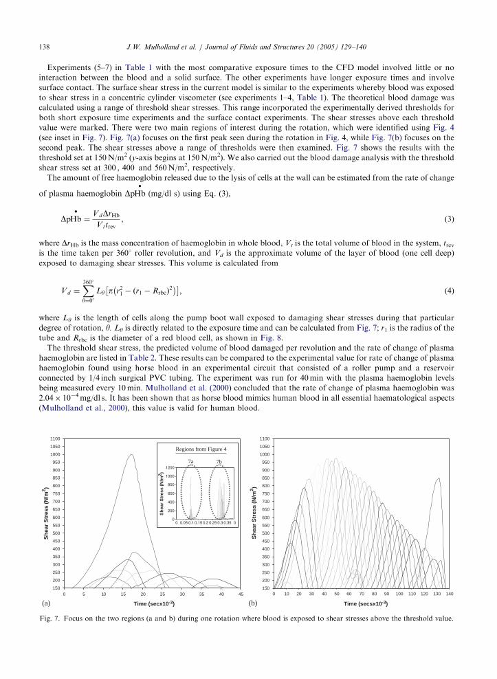
ARTICLE IN PRESSJ.W. Mulholland et al. / Journal of Fluids and Structures 20 (2005) 129–140138
Experiments (5–7) in Table 1 with the most comparative exposure times to the CFD model involved little or no
interaction between the blood and a solid surface. The other experiments have longer exposure times and involve
surface contact. The surface shear stress in the current model is similar to the experiments whereby blood was exposed
to shear stress in a concentric cylinder viscometer (see experiments 1–4, Table 1). The theoretical blood damage was
calculated using a range of threshold shear stresses. This range incorporated the experimentally derived thresholds for
both short exposure time experiments and the surface contact experiments. The shear stresses above each threshold
value were marked. There were two main regions of interest during the rotation, which were identified using Fig. 4
(see inset in Fig. 7). Fig. 7(a) focuses on the first peak seen during the rotation in Fig. 4, while Fig. 7(b) focuses on the
second peak. The shear stresses above a range of thresholds were then examined. Fig. 7 shows the results with the
threshold set at 150N/m2 (y-axis begins at 150N/m2). We also carried out the blood damage analysis with the threshold
shear stress set at 300 , 400 and 560N/m2, respectively.
The amount of free haemoglobin released due to the lysis of cells at the wall can be estimated from the rate of change
of plasma haemoglobin DpHbd
(mg/dl s) using Eq. (3),
DpHbd
¼VdDrHb
Vttrev; (3)
where DrHb is the mass concentration of haemoglobin in whole blood, Vt is the total volume of blood in the system, trevis the time taken per 3601 roller revolution, and Vd is the approximate volume of the layer of blood (one cell deep)
exposed to damaging shear stresses. This volume is calculated from
Vd ¼X360�y¼0�
Ly p r21 � ðr1 � RrbcÞ2
� �� ; (4)
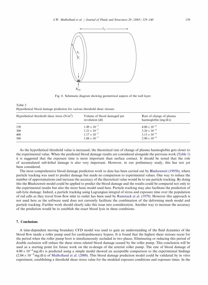
where Ly is the length of cells along the pump boot wall exposed to damaging shear stresses during that particular
degree of rotation, y. Ly is directly related to the exposure time and can be calculated from Fig. 7; r1 is the radius of the
tube and Rrbc is the diameter of a red blood cell, as shown in Fig. 8.
The threshold shear stress, the predicted volume of blood damaged per revolution and the rate of change of plasma
haemoglobin are listed in Table 2. These results can be compared to the experimental value for rate of change of plasma
haemoglobin found using horse blood in an experimental circuit that consisted of a roller pump and a reservoir
connected by 1/4 inch surgical PVC tubing. The experiment was run for 40min with the plasma haemoglobin levels
being measured every 10min. Mulholland et al. (2000) concluded that the rate of change of plasma haemoglobin was
2.04� 10�4mg/dl s. It has been shown that as horse blood mimics human blood in all essential haematological aspects
(Mulholland et al., 2000), this value is valid for human blood.
150
200
250
300
350
400
450
500
550
600
650
700
750
800
850
900
950
1000
1050
1100
0 10 20 30 40 50 60 70 80 90 100 110 120 130 140150
200
250
300
350
400
450
500
550
600
650
700
750
800
850
900
950
1000
1050
1100
0 5 10 15 20 25 30 35 40 45
(a) (b)
7a 7b
Sh
ear
Str
ess
(N/m
2 )
Regions from Figure 4
Sh
ear
Str
ess
(N/m
2 )
Sh
ear
Str
ess
(N/m
2 )
Time (secx10-3) Time (secsx10-3)
Fig. 7. Focus on the two regions (a and b) during one rotation where blood is exposed to shear stresses above the threshold value.
ARTICLE IN PRESS
Table 2
Hypothetical blood damage prediction for various threshold shear stresses
Hypothetical threshold shear stress (N/m2) Volume of blood damaged per
revolution (dl)
Rate of change of plasma
haemoglobin (mg/dl s)
150 1.49� 10�7 4.00� 10�4
300 1.21� 10�7 3.26� 10�4
400 1.17� 10�7 3.13� 10�4
560 1.08� 10�7 2.90� 10�4
L�
r1
Rrbc
Fig. 8. Schematic diagram showing geometrical aspects of the wall layer.
J.W. Mulholland et al. / Journal of Fluids and Structures 20 (2005) 129–140 139
As the hypothetical threshold value is increased, the theoretical rate of change of plasma haemoglobin gets closer to
the experimental value. When the predicted blood damage results are considered alongside the previous work (Table 1)
it is suggested that the exposure time is more important than surface contact. It should be noted that the role
of accumulated sub-lethal damage is also very important. However, in our preliminary study, this has not yet
been considered.
The most comprehensive blood damage prediction work to date has been carried out by Bludszuweit (1995b), where
particle tracking was used to predict damage but made no comparison to experimental values. One way to reduce the
number of approximations and increase the accuracy of the theoretical value would be to use particle tracking. By doing
this the Bludszuweit model could be applied to predict the blood damage and the results could be compared not only to
the experimental results but also the more basic model used here. Particle tracking may also facilitate the prediction of
sub-lytic damage. Indeed, a particle tracking using Lagrangian integral of stress and exposure time over the population
of red cells as they travel from flow inlet to outlet has been used by Ramstack et al. (1979). However this approach is
not used here as the software used does not currently facilitate the combination of the deforming mesh model and
particle tracking. Further work should clearly take this issue into consideration. Another way to increase the accuracy
of the prediction would be to establish the exact blood lysis in these conditions.
7. Conclusions
A time-dependent moving boundary CFD model was used to gain an understanding of the fluid dynamics of the
blood flow inside a roller pump used for cardiopulmonary bypass. It is found that the highest shear stresses occur for
the period when the roller pump boot is simultaneously occluded in two places. Eliminating or reducing this period of
double occlusion will reduce the shear stress related blood damage caused by the roller pump. This conclusion will be
used as a starting point for future work on the re-design of the arterial roller pump. The rate of blood damage of
4.00� 10�4mg/dl s is predicted using a simple model showed an acceptable comparison to the experimental findings
(2.04� 10�4mg/dl s) of Mulholland et al. (2000). This blood damage prediction model could be validated by in vitro
experiment, establishing a threshold shear stress value for the modeled exposure conditions and exposure times. In the

ARTICLE IN PRESSJ.W. Mulholland et al. / Journal of Fluids and Structures 20 (2005) 129–140140
future this information combined with the use of particle tracking would allow other models to be compared, as well as
the development of a more accurate blood prediction model.
References
Anderson, J.B., Wood, H.G., Allaire, P.E., Bearnson, G., Khanwildar, P., 2000. A computational flow study of the CF3 blood pump.
Artif Organs 24, 377–385.
Bernstein, E.F., Blackshear Jr., P.L., Keller, K.H., 1967. Factors influencing erythrocyte destruction in artificial organs. American
Journal of Surgery 114, 126–138.
Blackshear, P.L., Dorman, F.D., Steinbach, J.H., 1965. Some effects that influence hemolysis. Transactions—American Society for
Artificial Internal Organs 11, 112–117.
Bludszuweit, C., 1995a. Three-dimensional numerical prediction of stress loading of blood particles in a centrifugal pump. Artificial
Organs 19, 590–596.
Bludszuweit, C., 1995b. Model for general blood damage prediction. Artificial Organs 19, 583–589.
Bluestein, M., Mockros, L.F., 1969. Hemolytic effects of energy dissipation in flowing blood. Medical & Biological Engineering 7,
1–16.
Fung, Y.C., 1993. In Biomechanics, Mechanical Properties of Living Tissues, Second ed. Springer, Berlin.
Hansbro, S.D., Sharpe, D.A.C., Catchpole, R., 1999. Hemolysis during CPB: an in vivo comparison of standard roller pumps,
non-occlusive roller pumps and centrifugal pumps. Perfusion 14, 3–10.
Huang, C.R., Fabisiak, W., 1978. A rheological equation characterizing both the time dependent and the steady state viscosity of
whole human blood. American Institute of Chemical Engineers—Symposium Series, pp. 19-21.
Leverette, L.B., Hellums, J.D., Alfrey, C.P., Lynch, E.C., 1972. Red blood cell damage by shear stress. Biophysical Journal 12,
257–273.
Miyazoe, Y., Sawairi, T., Ito, K., Konishi, Y., Yamane, T., Nishida, M., Asztalos, B., Masuzawa, T., Tsukiya, T., Endo, S., Taenaka,
Y., 1999. Computational fluid dynamics analysis to establish the design process of a centrifugal blood pump: second report.
Artificial Organs 23, 762–768.
Miyazoe, Y., Sawairi, T., Ito, K., Konishi, Y., Yamane, T., Nishida, M., Masuzawa, T., Takiura, K., Taenaka, Y., 1998.
Computational fluid dynamic analyses to establish design process of centrifugal blood pumps. Artificial Organs 22, 381–385.
Mulholland, J.W., Massey, W., Shelton, J.C., 2000. Investigation and quantification of the blood trauma caused by the combined
dynamic forces experienced during cardiopulmonary bypass. Perfusion 15, 485–494.
Nakamura, S., Ding, W., Smith, W., Golding, L., 1999. Numeric flow simulation for an innovative ventricular assist system secondary
impeller. American Society for Artificial Internal Organs 45, 74–78.
Nevaril, C.G., Lynch, E.C., Alfrey, C.P., Hellums, J.D., 1968. Erythrocyte damage and destruction induced by shearing stress. Journal
of Laboratory Clinical Medicine 71, 784–790.
Nishida, M., Asztalos, B., Yamane, T., Masuzawa, T., Tsukiya, T., Endo, S., Taenaka, Y., Miyazoe, Y., Ito, K., Konishi, Y., 1999.
Flow visualization study to improve hemocompatibility of a centrifugal blood pump. Artificial Organs 23, 697–703.
Pinotti, M., Rosa, E.S., 1995. Computational prediction of hemolysis in a centrifugal ventricular assist device. Artificial Organs 19,
267–273.
Ramstack, J.M., Zuckerman, L., Mockros, L.F., 1979. Shear-induced activation of platelets. Journal of Biomechanics 12, 113–125.
Rooney, J.A., 1970. Hemolysis near an ultrasonically pulsating gas bubble. Science 16, 869–871.
Sallam, A.M., Hwang, N.H., 1984. Human red blood cell hemolysis in a turbulent shear flow: contribution of Reynolds shear stresses.
Biorheology 21, 783–797.
Sukumar, R., Athavale, M., Makhijani, V., Przekwas, A., 1996. Application of computational fluid dynamics techniques to blood
pumps. Artificial Organs 20, 529–533.
Sutera, S.P., Mehrjardi, M.H., 1975. Deformation and fragmentation of human RBC in turbulent shear flow. Biophysical Journal 15,
1–10.
Sutera, S.P., Croce, P.A., Mehrjardi, M.H., 1972. Hemolysis and subhemolytic alterations of human RBC induced by turbulent shear
flow. Transactions—American Society for Artificial Internal Organs 18, 335–341.
Takahama, T., Kanai, F., Hiraishi, M., Onishi, K., Yamazaki, Z., Suma, K., Asano, K., Kazama, M., 1985. Long-term non-
heparinized left heart bypass (LHB): centrifugal pump or roller pump. Transactions—American Society for Artificial Internal
Organs 31, 372–376.
Takiura, K., Masuzawa, T., Endo, S., Wakisaka, Y., Tatsumi, E., Taenaka, Y., Takano, H., Yamane, T., Nishida, M., Asztalos, B.,
Konishi, Y., Miyazoe, Y., Ito, K., 1998. Development of design methods of a centrifugal blood pump with in vitro tests, flow
visualization, and computational fluid dynamics: results in hemolysis tests. Artificial Organs 22, 393–398.
Williams, A.R., 1973. Shear-induced fragmentation of human erythrocytes. Biorheology 10, 303–311.
Williams, A.R., Hughes, D.E., Nyborg, W.L., 1970. Hemolysis near a transversely oscillating wire. Science 16, 871–873.
Wright, G., 1995. The assessment of pulsatile blood flow. Perfusion 10, 135–140.
Yarbourgh, K.A., Mockros, L.F., Lewis, F.J., 1966. Hydrodynamic hemolysis in extracorporeal machines. Journal of Thoracic and
Cardiovascular Surgery 52, 550–557.


