
ICES Report 04-39
A framework for the adaptive finite element solution
of large inverse problems. I. Basic techniques
Wolfgang Bangerth
Center for Subsurface Modeling, Institute for Computational Engineering andSciences, University of Texas at Austin; Austin TX 78712, USA
E-mail: [email protected]
Abstract. Since problems involving the estimation of distributed coefficients inpartial differential equations are numerically very challenging, efficient methods areindispensable. In this first part of a series, we will introduce a framework for theefficient solution of such problems. This comprises the use of adaptive finite elementschemes, efficient solvers for the large linear systems arising from discretization,and methods to treat additional information in the form of inequality constraintson the parameter sought. The methods to be developed will be based on an all-at-once approach, in which the inverse problem is solved through a Lagrangianformulation. In order to allow for discretizations that are adaptively refined asnonlinear iterations proceed, all algorithms are formulated in a continuous function-space setting. Numerical examples will demonstrate the applicability of the methodfor problems with several million unknowns and more than 10,000 parameters.
This article also defines the notation and basic methods used in subsequent parts todevelop a posteriori error estimates, upon which optimal discretizations will be based.
Submitted to: Inverse Problems
1. Introduction
Parameter estimation methods are important tools in cases where quantities we would
like to know cannot be measured directly, but where only measurements of related
quantities, so-called observables, are available. This relation between parameter and
observable is usually called the equation of state. The goal of parameter estimation
is then to recover the unknown quantity from measurements of observables, using the
state equation.
If the state equation is a differential equation, such parameter estimation problems
are commonly referred to as inverse problems. These problems have a vast number of
applications. For example, identification of the underground structure (e.g. the elastic
properties, density, electric or magnetic permeabilities of the earth) from measurements
at the surface or in boreholes, or of the groundwater permeability of a soil from
measurements of the hydraulic head fall in this class. Likewise, detecting cracks

A framework for adaptive FEM for large inverse problems 2
in materials, computer tomography, and electrical impedance tomography in medical
imaging can be cast as inverse problems.
In particular, we will consider cases where we make many experiments to identify
the parameters. Here, by an experiment we mean subjecting the physical system to
a certain forcing and measuring its response. For example, in computer tomography,
a single experiment would be characterized by irradiating a body from a given angle
and measuring the transmitted part of the radiation; the multiple experiment situation
is characterized by using data from various incidence angles and trying to find a set
of parameters that matches all the measurements at the same time (joint inversion).
Likewise, in geophysics, a single experiment would be placing a seismic source somewhere
and measuring reflection data at various receiver position; the multiple experiment case
is taking into account data for more than one source position. We may also want to
include other types of data on the same region, say magnetotelluric or gravimetry data
for a joint, multi-physics inversion scenario.
This series of papers is devoted to the development of efficient techniques for
the solution of such inverse problems where the state equation is a partial differential
equation (henceforth abbreviated as PDE), and the parameters to be determined are
one or several distributed functions. It is well-known that the numerical solution of PDE
constrained inverse or optimization problems is significantly more challenging than that
of a PDE alone, since the optimization procedure is usually iterative and in each iteration
may need the numerical solution of a large number of partial differential equations. In
some applications, several ten or hundred thousand solutions of linearized PDEs are
required to solve the inverse problem, and each PDE may be discretized by up to several
hundred thousand unknowns.
It is thus obvious that efficiency of solution is a major concern. In this and following
papers, we will devise adaptive finite element techniques that significantly reduce the
numerical effort needed to solve such problems. Adaptive methods are now commonly
accepted as necessary ingredients of present finite element solvers for partial differential
equations. However, they have not yet found their way into the numerical solution
of distributed inverse problems, and are only slowly adopted in the solution of PDE
constrained optimization, see for example [10, 9, 27]. In this paper, we lay the necessary
algorithmic and mathematical foundations for a framework in which adaptive meshing
is an integral part. It will be used to derive error estimates in later parts of the series,
which we will then in turn use to drive automatic mesh refinement.
The goal of the present work is thus to develop a general framework for the efficient
solution of PDE constrained inverse problems. The main ingredients will be:
• formulation of all algorithms in function spaces, i.e. before rather than after
discretization, since this gives us more flexibility in discretizing as iterations
proceed, and resolves all scaling issues once and for all;
• the use of adaptive finite element techniques with mesh refinement based on a
posteriori error estimates;

A framework for adaptive FEM for large inverse problems 3
• the use of different meshes for the discretization of different quantities, for example
of state variables and of parameters, in order to reflect their respective properties;
• the use of Newton-type methods for the outer (nonlinear) iteration, and of efficient
linear solvers for the Newton steps;
• the use of approaches that allow for the parallelization of work, yielding subproblems
that are equivalent to only forward and adjoint problems;
• the inclusion of pointwise bounds on the parameters into the solution process.
Except for the derivation of error estimates, which will be discussed in a subsequent
part of this series, we will discuss all these building blocks, and will show that these
techniques allow us to solve problems of the size outlined above. It should be stressed
that the formulation of algorithms in function spaces is indispensable if we want to use
successively finer discretizations, since otherwise quantities computed on one grid would
not be comparable to one after mesh refinement.
We envision that the techniques to be presented are used for relatively complex
problems. We will thus state them in a general setting, and in this paper present their
application to a simple model case for brevity of exposition. However, the algorithms
will be designed for efficiency, and will not make use of the relative simplicity of the
model problem. More complex examples will then be treated in following parts of this
series.
Solving large-scale multiple-experiment inverse problems requires algorithms on
several levels, all of which have to be taylored to high efficieny. In this article, we will
review the building blocks of a framework for this:
• formulation as a Lagrangian optimization problem with PDE constraints (Section
2); a model problem is given in Section 3;
• outer nonlinear solution by a Gauss-Newton method posed in function spaces
(Section 4);
• discretization of each Newton step by finite elements on independent meshes
(Section 5);
• linear Schur complement solvers for the resulting discrete systems (Section 6);
• methods to incorporate bound constraints on the parameters sought (Section 7)
In Section 8, we will present numerical examples. We will draw conclusions in the final
section.
In subsequent papers of this series, the derivation of mesh refinement criteria based
on a posteriori error estimates for energy-type and general output-type quantities will
be discussed, and the application of all these techniques to more complex problems will
be demonstrated.
2. General formulation and notation
Let us begin by introducing some abstract notation, which we will use for the derivation
of the entire scheme. This, above all, concerns the set of parameters, state equations,
A framework for adaptive FEM for large inverse problems 4
measurements, regularization, and the introduction of an abstract Lagrangian.
Let us note that some of the formulas below will become cumbersome to read
because of the number of indices. To understand their meaning, it is often helpful
to imagine we had only a single experiment (for example, only one incidence angle in
tomography, or only one source position in seismic imaging). In this case, drop the
index i on first reading, as well as all summations over i.
State equations
Let the general setting of the problems we consider be as follows: assume we have a
physical situation that is described by a number i = 1, . . . , N of (independent) partial
differential equations posed on a domain Ω ⊂ Rd:
Ai[q] ui = f i in Ω, (1)
Bi[q] ui = hi on ΓiN ⊂ ∂Ω, (2)
ui = gi on ΓiD = ∂Ω\Γi
N , (3)
where Ai[q] are partial differential operators that depend on a set of a priori unknown
distributed coefficients q = q(x) ∈ Q, x ∈ Ω, and Bi[q] are boundary operators that may
also depend on the coefficients. f i, hi and gi are right hand sides and boundary values,
respectively, of which we assume that they are known, and that do not depend on the
coefficients q. The functions ui are the solutions of the partial differential equations,
and are assumed to be from spaces V ig = ϕ ∈ V i : ϕ|Γi
D= gi. These solutions
can be vector valued, but we assume that solutions ui, uj of different equations i 6= j
do not couple except for their dependence on the same set of parameters q. We also
assume that the solutions to each of the differential equations is unique for every given
set of parameters q in a subset Qad ⊂ Q of physically meaningful values, for example
Qad = q ∈ L∞(Ω) : q0 ≤ q(x) ≤ q1.Typical cases we have in mind would be a Laplace-type equation when we are
considering electrical impedance tomography or gravimetry inversion, or Helmholtz or
wave equations in case we are looking at inverting seismic or magnetotelluric data.
The set of parameters q would, in these cases, be electrical conductivities, densities,
or elasticity coefficients. If we have done several measurements for the identification
of the same parameters, but with different source terms, at different frequencies, or in
an otherwise different setting, then we will identify each of these experiments with one
index i = 1, . . . , N . The operators Ai may be the same for several experiments, but if
we use different physical effects (for example gravimetry and seismic data) to identify
the same parameters – the so-called multi-physics inversion case – then they will be
different.
The formulation above may easily be extended also to the case of time-dependent
problems, but we omit this for brevity. Likewise, the case that the parameters are a
finite number of scalar values is included as a simple special case, but will not be the
main focus of our work.

A framework for adaptive FEM for large inverse problems 5
For treatment in a Lagrangian setting in function spaces as well as for discretization
by finite elements, it is necessary to formulate the state equations (1)–(3) in a variational
form. For this we assume that the solutions ui ∈ V ig are solutions of the following
variational equalities:
Ai(q;ui)(ϕi) = 0 ∀ϕi ∈ V i0 , (4)
where V i0 = ϕi ∈ V i : ϕi|Γi
D= 0. The semilinear form Ai : Q× V i
g × V i0 → R may be
nonlinear in its first set of arguments, but is linear in the test function, and includes the
actions of the domain and boundary operators Ai and Bi, as well as the inhomogeneous
terms. We assume that the Ai are differentiable. Again, extensions to more complicated
problems are possible, but are omitted for brevity.
Below, we will introduce a model problem for the Laplace equation. In this
particular case, Ai[q]ui = −∇ · (q∇ui), Bi[q]ui = q∂nui, and
A(q;ui)(ϕi) = (q∇ui,∇ϕi)Ω − (f, ϕi)Ω − (g, ϕi)ΓN.
Measurements
In order to determine the unknown quantities q, we have measurements of (parts of)
each of the state variables ui, or of derived quantities. For example, we might have
measurements of the value at certain points, averages on subdomains, or gradients.
Let us denote the space of measurements of the ith state variable by Z i, and let
M i : V ig → Z i be the measurement operator, i.e. the operator that extracts from the
state solution ui the measurement values.
Reconstruction of the coefficients q will then be accomplished by finding those
coefficients, for which the expected measurements M iui match the actual measurements
zi ∈ Z i best. We will measure this comparison using a convex, differentiable functional
m : Z i → R+ with m(0) = 0. In many cases, m will simply be an L2 norm on Z i, but
more general functionals are allowed, for example to suppress the effects of non-Gaussian
noise.
Examples of common measurement situations for scalar valued solutions are:
• L2 measurements of values: If measurements on a set Σ ⊂ Ω are available, then
M i is the embedding operator from V ig into Z i = L2(Σ), and the quantity to be
minimized is
mi(M iui − zi) =1
2‖ui − zi‖2
L2(Σ).
As special cases, Σ can be the whole domain Ω, or its boundary ∂Ω. The case
of distributed measurements occurs in situations where a measuring device can be
moved around to every point of Σ, for example a laser scanning a membrane, or
imaging radiation on a photographic film.
• Point measurements: If we have S measurements of u(x) at positions xs ∈ Ω, s =
1, . . . , S, then Z i = RS, and (M iui)s = u(xs). If we take again a quadratic norm
A framework for adaptive FEM for large inverse problems 6
on Z i, then for example
mi(M iui − zi) =1
2
S∑s=1
|ui(xs)− zis|2
is a possible choice. The case of point measurements is frequent in applications
where a small number of stationary measurement devices is used, for example
seismometers in seismic data assimilation.
• Gradient measurements: If we only have measurements of the gradient, then
M i = ∇, Z i = (L2)d, and we can for example choose
mi(M iui − zi) =1
2‖∇ui − zi‖2
L2(Ω).
An example for this is measuring the gravitational pull of a body, which is the
gradient of the gravimetric potential.
Other choices are of course possible, and are usually dictated by the type of available
measurements.
We will in general assume that the M i are linear, but there are applications where
this is not the case. For example, in some applications only statistical correlations of ui
are known, or a power spectrum. Extending the algorithms below to nonlinear M i is
straightforward, but we omit this for brevity.
Regularization
Since inverse problems are often ill-posed, regularization is needed to suppress unwanted
features in solutions q. In this work, we include it by using a Tikhonov regularization
term involving a convex differentiable regularization functional r : Q → R+, see for
example [26]. r is usually chosen to be the square of a quadratic seminorm on Q, for
example r(q) = 12‖∇t(q − q)‖2
L2(Ω) with an a priori guess q and some t ∈ N+. Other
popular choices are smoothed versions of bounded variation seminorms [20, 17, 19].
As above, the type of regularization is usually dictated by the application and insight
into physical and unphysical features of solutions. It may also be chosen to give the
misfit functional a proper meaning, for example in the point value case where we need
a continuous solution. An additional regularization functional may be used if different
distributed parameters, e.g. the two Lame constants, are assumed to share structural
properties such as locations of discontinuities (see, e.g., [23]).
Characterization of solutions
The goal of the inverse problem is to find that set of physical parameters q ∈ Qad for
which the observations M iui of the resulting state variables would match the actual
observations zi best. We formulate this as the following constrained minimization
problem over ui ∈ V ig , q ∈ Qad:
minimize J(ui, q) =N∑
i=1
σimi(M iui − zi) + βr(q) (5)

A framework for adaptive FEM for large inverse problems 7
such that Ai(q;ui)(ϕi) = 0 ∀ϕi ∈ V i0 , 1 ≤ i ≤ N.
Here, σi > 0 are factors weighting the relative importance of individual measurements,
and β > 0 is a regularization parameter. As the choice of these constants is a topic of
its own, we assume their values as given within the scope of this work.
In order to characterize solutions to (5), let us subsume the individual solutions ui
to a vector u, and likewise denote the spaces V ig , V
i0 by the components of spaces Vg,V0.
Furthermore, we introduce a set of Lagrange multipliers λ ∈ V0, and denote the joint
set of variables by x = u,λ, q ∈ Xg = Vg ×V0 ×Q.
We assume that solutions of problem (5) can be characterized as stationary points
of the following Lagrangian L : Xg → R, which couples the functional J : Vg×Q → R+
defined above to the state equation constraints through Lagrange multipliers λi ∈ V i0 :
L(x) = J(u, q) +N∑
i=1
Ai(q;ui)(λi). (6)
Solutions are then stationary points of this Lagrangian, i.e. the optimality conditions
read in abstract form
Lx(x)(y) = 0 ∀y ∈ X0, (7)
where the semilinear form Lx : Xg×X0 → R is the differential of the Lagrangian L, and
X0 = V0×V0×Q. Indicating derivatives of functionals with respect to their arguments
by subscripts, we can expand (7) to yield the following set of nonlinear equations:
Lλi(x;ϕi) ≡ Ai(q;ui)(ϕi) = 0 ∀ϕi ∈ V i0 , (8)
Lui(x;ψi) ≡ σimiu(M
iui − zi)(ψi) + Aiu(q;u
i)(ψi, λi) = 0 ∀ψi ∈ V i0 , (9)
Lq(x;χ) ≡ βrq(q)(χ) +N∑
i=1
Aiq(q;u
i)(χ, λi) = 0 ∀χ ∈ ∂Q. (10)
The first set of equations denotes the state equations for i = 1, . . . , N ; the second the
adjoint equations defining the Lagrange multipliers λi; finally, the third is the control
equation holding for all functions from the tangent space ∂Q to Q at the solution q.
Note that we have included the (linear) constraint of Dirichlet boundary values into the
function space where we look for solutions, rather than the Lagrange functional. We do
so, since we can simply set an initial iterate in the solution of this nonlinear system to
these boundary values. Further updates to this iterate are then sought from the vector
space with zero boundary conditions.
The question whether the solution of the original constrained optimization problem
(5) can indeed be characterized by the stationarity of a Lagrangian, (7), depends
crucially on the exact form of the various functionals involved, and the function spaces
Vg and Q and cannot be answered in general. It holds for a large number of practical
applications (see, for example, [8]), and we assume that this augmentability holds also
for the cases discussed in this work.

A framework for adaptive FEM for large inverse problems 8
3. A model problem
As a simple model problem which we will use to give the abstract results of this work
a more concrete form, we will consider the following situation: assume we intend to
identify the coefficient q in the (single) elliptic PDE
−∇ · (q∇u) = f in Ω, u = g on ∂Ω, (11)
and that measurements are the values of the solution u everywhere in Ω, i.e. we choose
m(Mu − z) = m(u − z) = 12‖u − z‖2
L2(Ω). This situation can be considered as a
mathematical description of a membrane with variable stiffness q(x) which we try to
identify by subjecting it to a known force f and clamping it at the boundary with
boundary values g. This results in displacements of which we obtain measurements
z everywhere. For simplicity, we have here chosen to consider only one experiment,
i.e. N = 1.
For this situation, Vg = u ∈ H1 : u|∂Ω = g, Q ⊂ L∞. Choosing σ = 1, the
Lagrange functional then has the form
L(x) = m(u− z) + βr(q) + (q∇u,∇λ)− (f, λ).
With this, the optimality conditions (8)–(10) read in weak form
(q∇u,∇ϕ) = (f, ϕ), (12)
(q∇ψ,∇λ) = −(u− z, ψ), (13)
βrq(q;χ) = −(∇u,∇λ), (14)
and have to hold for all test functions ϕ, ψ, χ ∈ V 10 × V 1
0 ×Q = H10 ×H1
0 ×Q. The
first of these is the state equation, the second the adjoint one.
4. Nonlinear solvers
The stationarity conditions (7) form a set of nonlinear partial differential equations that
has to be solved iteratively, for example using Newton’s method, or a variant thereof.
In this section, we will formulate the Gauss-Newton method in function spaces. The
discretization of each step by adaptive finite elements will then be presented in the next
section, followed by a discussion of solvers for the resulting linear systems.
Since there is no need to compute the initial nonlinear steps on a very fine grid
when we are still far away from the solution, we will want to use successively finer
meshes as we approach the solution. In order to make quantities computed on different
meshes comparable, all of the following algorithms will be formulated in a continuous
setting, and only then be discretized. This also answers once and for all questions about
the correct scaling of weighting matrices in misfit and regularization functionals, as
discussed for example in [2], even if we choose locally refined grids, as they will appear
naturally upon discretization. In this section, we indicate a Gauss-Newton procedure,
i.e. determination of search direction and step length, in infinite dimensional spaces,
and discuss in the next section its discretization by a finite element scheme. It is

A framework for adaptive FEM for large inverse problems 9
worth noting that the number of possible methods for solving such problems is vast
[24, 1, 31, 28, 22, 29, 16].
However, we believe that the Gauss-Newton method is particularly suited since
it allows for scalable algorithms even with large numbers of experiments, and large
numbers of degrees of freedom both in the discretization of the state equations as well
as of the parameter. Comparing this method to a pure Newton method, it allows for
the use of more efficient linear solvers for the discretized problems, see Section 6. In
addition, the Gauss-Newton method has been shown to have better stability properties
for parameter estimation problems than the Newton method, see [15, 14].
Search directions
Given a present iterate xk = uk,λk, qk ∈ X , the first task of any method is to compute
a search direction δxk = δuk, δλk, δqk ∈ Xδg, in which we seek the next iterate xk+1.
The Dirichlet boundary values δg of this update are chosen as δuik|ΓD
= gi − uik|ΓD
,
δλik|ΓD
= 0, bringing us to the exact boundary values if we take a full step.
In order to determine the search direction, we use the Gauss-Newton method. In
the present case, we determine updates δuk, δqk by minimizing the following quadratic
approximation to J(·, ·) with linearized constraints:
minδuk,δqk
J(uk, qk) + Ju(uk, qk)(δuk) + Jq(uk, qk)(δqk)
+1
2Juu(uk, qk)(δuk, δuk) +
1
2Jqq(uk, qk)(δqk, δqk) (15)
s.t. Ai(qk;uik)(ϕ
i) + Aiu(qk;u
ik)(δu
ik, ϕ
i) + Aiq(qk;u
ik)(δqk, ϕ
i) = 0,
where the linearized constraints are understood to hold for 1 ≤ i ≤ N and for all test
functions ϕi ∈ V i0 . The solution of this problem provides us with updates δuk, δqk for
the state variables and the parameters. The updates for the Lagrange multiplier δλk
are not determined by the Gauss-Newton step at first. However, the solution of (15) is
characterized by coupling the linearized constraints to the quadratic function. It turns
out that we can get updates δλk for the original problem, by using λk +δλk as Lagrange
multiplier for the constraint of the Gauss-Newton step (15). Bringing the terms with
λk to the right hand side, the updates are then characterized by the following system
of linear equations:
σimiuu(M
iuik − zi)(δui
k, ϕi) + Ai
u(qk;uik)(ϕ
i, δλik) = −Lui(xk)(ϕ
i)
Aiu(qk;u
ik)(δu
ik, ψ
i) + Aiq(qk;u
ik)(δq
ik, ψ
i) = −Lλi(xk)(ψi) (16)∑
i
Aiq(qk;u
ik)(χ, δλ
ik) + βrqq(qk)(δqk, χ) = −Lq(xk)(χ),
for all test functions ϕi, ψi, χ. The right hand side of these equations are the negative
gradient of the original Lagrangian, given already in the optimality condition (8)–(10).
The matrix structure of this system will be given in the next section, showing
a number of nice properties. Note that the equations determining the updates for
the ith experiment decouple from all other experiments, except for the last equation.

A framework for adaptive FEM for large inverse problems 10
This will allow us to solve them mostly separated, and in particular it allows for
simple parallelization by placing the description of different experiments onto different
machines. Furthermore, the first and second equations can be solved sequentially.
In order to illustrate these equations, we state their form for the model problem of
Section 3. In this case, the above system reads
(δuk, ϕ) + (∇δλk, qk∇ϕ) = −Lu(xk)(ϕ),
(∇ψ, qk∇δuk) + (∇ψ, δqk∇uk) = −Lλ(xk)(ψ),
(∇δλk, χ∇uk) + βrqq(qk)(δqk, χ) = −Lq(xk)(χ),
with the right hand sides being the gradient of the Lagrangian given in Section 3.
In general, this continuous Gauss-Newton direction will not be computable
analytically. We will therefore approximate it by a finite element function δxk,h, as
discussed in the next section.
As a final remark, let us note that the pure Newton’s method would read
Lxx(xk)(δxk, y) = −Lx(xk)(y) ∀y ∈ X0, (17)
where Lxx(xk)(·, ·) denotes the bilinear form of second variational derivatives of the
Lagrangian L at position xk. The Gauss-Newton method can alternatively be obtained
from this by simply dropping all terms that are proportional to the Lagrange multiplier
λk. The reasoning for this is that we expect the Lagrange multiplier to be small for
small-noise problems, a fact that is warranted by looking at (9): the Lagrange multiplier
has to satisfy an equation with a term proportional to Mu− z as right hand side; thus,
assuming stability of the (linear) adjoint operator, it will be small if the residual is small
at the solution.
Step lengths
Once we have a search direction δxk, we have to decide how far to go in this direction
starting at xk to obtain the next iterate xk+1 = xk +αkδxk. In constrained optimization,
a merit function including the minimization functional J(·) as well as the violation of
the constraints is usually used. One particular problem here is the infinite dimensional
nature of the state equation constraint, with the residual of the state equation being
in the dual space, V ′0 , of V0 (which, for the model problem, is H−1). This places some
restrictions on the types of merit functions that can practically be used.
In order to avoid these problems, we simply use the norm of the residual of the
optimality condition (7) on the dual space of X0 as merit function:
p(α) =1
2‖Lx(xk + αδxk)(·)‖2
X ′0≡ 1
2supy∈X0
[Lx(xk + αδxk)(y)]2
‖y‖2X0
.
We will show in the next section that we can give a simple-to-compute lower bound for
this norm using the discretization we already employ for the computation of the search
direction.
The following lemma shows that this merit function is actually useful:

A framework for adaptive FEM for large inverse problems 11
Lemma 1 The merit function p(α) is valid, i.e. Newton directions are directions of
descent, p′(0) < 0. Furthermore, if xk is a solution of the parameter estimation problem,
then p(0) = 0. Finally, in the vicinity of the solution, full steps are taken, i.e. α = 1
minimizes p.
Proof. We prove the lemma for the special case of only one experiment (N = 1)
and that X = H10 × H1
0 × L2, i.e. the situation of the model example. In this case,
there is a representation gu(xk + αδxk) = Lu(xk + αδxk)(·) ∈ H−1, gλ(xk + αδxk) =
Lλ(xk +αδxk)(·) ∈ H−1, and gq(xk +αδxk) = Lq(xk +αδxk)(·) ∈ L2. The dual norm of
Lx can then be written as
‖Lx‖2X ′
0=⟨gu, (−∆)−1gu
⟩+⟨gλ, (−∆)−1gλ
⟩+ (gq, gq),
where (−∆)−1 : H−1 → H10 , and 〈·, ·〉 indicates the duality pairing between H−1 and
H10 . Then,
p′(0) =⟨guu(δuk), (−∆)−1gu
⟩+⟨gλλ(δλk), (−∆)−1gλ
⟩+ (gqq(δqk), gq),
where gux(δxk) is the derivative of gu in direction δxk, i.e. the functional of second
derivatives of L. However, by definition of the Newton direction, (17), this is equal to
the negative gradient, i.e.
p′(0) = −‖Lx(xk)‖2X ′
0= −2p(0) < 0.
Thus, Newton directions are directions of descent for this merit function.
The second part of the lemma is obvious by noting the optimality condition (7).
The last part follows by noting that near the solution the Lagrangian (and thus the
function p(α)) is well approximated by a quadratic function if the various functionals
involved in the Lagrangian are sufficiently smooth.
Although the lemma technically does not cover the case of Gauss-Newton search
directions, all numerical experiments indicate that the results also hold for this case, at
least in the case of small noise.
5. Discretization
In order to compute finite-dimensional approximations to the solution of the parameter
estimation problem, we have to discretize both the state and adjoint variables, as well
as the parameters. Here, we will choose finite element schemes to do so, and we will use
subsequently finer meshes on subsequent Gauss-Newton iterations, to make the initial
iterations cheaper. In each iteration, we define finite element spaces Xh ⊂ X over
triangulations in the usual way. For these grids and spaces, we assume the following
requirements:
• Nesting: The mesh Tik to be used in the discretization of the ith state equation in
step k must be obtainable from Tik−1 by hierarchic coarsening and refinement. This
greatly simplifies operations like evaluation of the right hand side of the Newton
direction equation, Lx(xk)(·) for all discrete test functions, but also the update
operation xk+1 = xk + αkδxk,h.

A framework for adaptive FEM for large inverse problems 12
• State vs. parameter meshes: Independently of the meshes Tik used for the
discretization state equations, a mesh Tqk will be used to discretize the parameters
q on step k. This reflects that the regions of missing regularity of parameters
and state variables need not necessarily coincide. We may also use different
discretization spaces for parameters and state/adjoint variables, for example spaces
of discontinuous functions for quantities like density or elasticity coefficients. We
will require that each of the ‘state meshes’ Tik can be obtained by hierarchical
refinement from the ‘parameter mesh’ Tqk.
Although obvious, both the choice of independent grids for state and parameter meshes,
as well as the adaptive choice of subsequently finer meshes, have apparently not been
used in the literature to the author’s best knowledge. Both techniques offer the
prospect of greatly reducing the amount of numerical work. We will see that with the
requirements on the meshes above, the additional work associated with using different
meshes is very small.
Here, the basic idea in choosing subsequently finer meshes is that as we are still far
away from the solution, we can work on coarser meshes for approximating the Newton
steps, and only go over to finer ones as we approach the solution. Most of the initial
steps will therefore contribute only negligibly to the total cost of the solution process,
both because they are relatively small problems, but also because a smaller size reduces
the ill-posedness, making the iterative solution of the linear problems faster. In addition,
choosing coarse meshes for the first iterates also stabilizes the problem on the initial
steps, when we are still far away from the solution, effectively acting as an additional
regularization.
Choosing different ‘state’ and ‘parameter meshes’ also allows for problems where the
parameters do not require high resolution, or only in certain areas of the domain, while
the state equation requires this. A typical problem would be high-frequency tomography,
where the coefficient sought might be a function that is constant in large parts of the
domain, while the high-frequency oscillations of state and adjoint variables require a
fine grid everywhere where these variables have a significant value. Again, being able
to reduce the number of parameters compared to the number of state variables, and
localizing them at places where enough information is available for their reconstruction,
reduces the numerical work and improves conditioning of the subproblems.
In the next few paragraphs, we will briefly describe the process of discretizing the
equations for the search directions and the choice of the step length. We will then give
a brief note on the criteria for generating the meshes on which we discretize.
Search directions
By choosing a finite dimensional subspace Xh = Vh×Vh×Qh ⊂ X , we obtain a discrete
counterpart for equation (16) describing the Gauss-Newton search direction:
σimiuu(M
iuik − zi)(δui
k,h, ϕih) + Ai
u(qk;uik)(ϕ
ih, δλ
ik,h) = −Lui(xk,h)(ϕ
ih),
Aiu(qk;u
ik)(δu
ik,h, ψ
ih) + Ai
q(qk;uik)(δq
ik,h, ψ
ih) = −Lλi(xk,h)(ψ
ih),(18)

A framework for adaptive FEM for large inverse problems 13∑i
Aiq(qk;u
ik)(χh, δλ
ik,h) + βrqq(qk)(δqk,h, χh) = −Lq(xk,h)(χh),
Note that if the discretization we use does not involve stabilization terms, then
discretization and differentiation commute, so (18) can either be viewed as the
discretization of the continuous Gauss-Newton step (16), or as one step for a discretized
version (on a fixed mesh) of the Gauss-Newton step problem (15). We prefer the first
view, since it allows more intuitively to change the meshes between iterations.
Choosing a basis for the space Xh, we can write (18) in matrix form as follows: M AT 0
A 0 C
0 CT βR
δuk,h
δλk,h
δqk,h
=
Fu
Fλ
Fq
. (19)
Since the individual state equations and variables do not couple across experiments,
M = diag(Mi) and A = diag(Ai) are block diagonal matrices, with the diagonal
blocks stemming from second derivatives of the misfit functionals, and of the tangential
operators of the state equations, respectively. They are equal to
(Mi)kl = miuu(M
iuik − zi)(ϕi
k, ϕil), (Ai)kl = Ai
u(xk)(ϕil, ϕ
ik),
where ϕil are test functions for the discretization of the ith state equation. Likewise,
C = [C1, . . . ,CN ] is defined by
(Ci)kl = Aiq(xk)(χ
ql , ϕ
ik),
with χql being discrete test functions for the parameters q, and (R)kl = rqq(qk)(χ
qk, χ
ql ).
The evaluation of Ci may be difficult since it involves shape functions from different
meshes and finite element spaces. However, since we have required that Tik can be
obtained from Tqk by hierarchical refinement, we can represent each shape function χq
k
on the parameter mesh as a sum over respective shape functions χis on each of the state
meshes: χqk =
∑s Xi
ksχis. Thus, Ci = CiXi, with Ci built with shape functions from
only one grid. The matrix Xi is fairly simple to generate because of the hierarchical
structure of the meshes. In general, it is worthwhile to store Ci and Xi separately,
rather than forming Ci explicitly.
Note that if we had wanted to use the full Newton search direction instead of the
Gauss-Newton one, then the top right and bottom left blocks of the matrix in (19) would
also be nonzero. In addition, if the state equations were nonlinear in ui or qi, additional
terms would have to be added to the M and R blocks.
Step lengths
Since step length selection is only a tool for seeking the exact solution, we may be
content with approximating the merit function p(α) introduced in Section 4. To this
end, we use a lower bound p(α) for p(α), by restricting the set of possible test functions
to the discrete space Xh which we are already using for the discretization of the search
direction:
p(α) =1
2supy∈Xh
[Lx(xk + αδxk)(y)]2
‖y‖2X0
≤ 1
2‖Lx(xk + αδxk)(·)‖2
X ′0
= p(α).

A framework for adaptive FEM for large inverse problems 14
By selecting a basis of Xh, p(α) can be computed by linear algebra. For example, for
the single experiment case (N = 1) and if X = H10 ×H1
0 × L2, we have that
p(α) =1
2
[⟨gu(α), Y −1
1 gu(α)⟩
+⟨gλ(α), Y −1
1 gλ(α)⟩
+⟨gq(α), Y −1
0 gq(α)⟩],
where (Y0)kl = (χk, χl), (Y1)kl = (∇ϕk,∇ϕl) are mass and Laplace matrices,
respectively. The gradient vectors are (gu)l = Lu(xk + αδxk)(ϕl), and correspondingly
for gλ and gq. Here, ϕl are again basis functions from the discrete approximation space
to the state and adjoint variable, and χl for the parameters.
The evaluation of p(α) therefore requires only two inversions of Y1 per experiment,
and of one mass matrix for the parameters. Setting up the gradient vectors reuses
operations that are also available from the generation of the linear system in each
Gauss-Newton step. With this merit function, the computation of a step length is then
done using the usual methods (see, e.g., [30]). Compared to the effort required for the
solution of the Newton step, the effort for line search is usually negligible, in particular
since not many evaluations of p will be necessary. However, numerical experiments
indicate that the effort can be further reduced by approximating Y0, Y1, for example by
only considering their diagonal elements; however, the main feature of correctly scaling
degrees of freedom corresponding to cells of different size should be preserved in schemes
with adaptively chosen meshes.
Mesh refinement
As noted, we may choose different grids for each Newton step. For practical purposes,
these meshes should share a minimum of characteristics, as described above, but apart
from that their generation is arbitrary. For the numerical examples presented in this
paper, the meshes are kept constant for a number of nonlinear iterations until we are
satisfied with the progress of the nonlinear iterations. The meshes are then refined
using simple smoothness indicators to refine both the meshes for the state and adjoint
variables, as well as for the parameter. In subsequent parts of this series, we will derive
error estimates for the inverse problem, and generate refinement criteria from them.
Also, the process of evaluating the progress of iterations on a grid will be discussed in
more detail.
6. Linear solvers
The linear system (19) is hardly solvable as is, except for the most simple problems. This
is due to its size, which is twice the number of variables in each discrete forward problem,
summed up over all experiments. Furthermore, it is indefinite and often extremely ill-
conditioned (see [4]): if the state equations are the simple Poisson equations of the
model problem, then the condition number of the matrix grows with the mesh size h as
O(h−4) (for a misfit functional m(ϕ) = 12‖∇ϕ‖2) or even O(h−6) (for m(ϕ) = 1
2‖ϕ‖2)!
This, and the size of the problem makes both solution by direct as well as iterative

A framework for adaptive FEM for large inverse problems 15
methods very hard or impossible for the large problems arising if many experiments are
involved; for discussions of various approaches for such problems see, e.g., [18, 21, 3, 13].
However, we can re-state the system of equations by block elimination and use of
the sub-structure of the individual blocks to obtain the following Schur complement
formulation:
S δqk,h = Fq −N∑
i=1
CiTAi−T(Fi
u −MiAi−1Fi
λ), (20)
Ai δuik,h = Fi
λ −Ciδqk,h, (21)
AiT δλik,h = Fi
u −Miδqk,h, (22)
where S denotes the Schur complement
S =(βR +
N∑i=1
CiTAi−TMiAi−1
Ci). (23)
These equations are much simpler to solve, mainly for their size and their structure:
For the second and third equations, which are linearized forward and adjoint problems,
efficient solvers are usually available. Since the equations for the individual experiments
are separated, they can also be solved in parallel. The system in the first equation,
(20), is small, its size being equal to the number #δqk,h of discretized parameters δqk,h,
which is much smaller than the total number of degrees of freedom and in particular
independent of the number of experiments. Furthermore, S has some nice properties:
Lemma 2 The Schur complement matrix S is symmetric and positive definite if at least
one of the matrices R or M as defined above is positive definite.
The proof of this lemma is trivial, noting that both R and M stem from second
derivatives of convex functionals, and are thus already at least positive semidefinite.
Regarding the actual solution of this equation, we note that one may build up an
actual representation of the matrix S. This would involve #δqk,h linearized forward and
backward solutions for each experiment, which is usually too expensive as we anticipate
#δqk,h to be in the range of thousands, or even more. However, by consequence of
the lemma, we can use well-known and fast iterative methods for the solution of this
equation, such as the Conjugate Gradient method. In each matrix-vector multiplication
we would then have to perform one linearized forward and one backward step for each
experiment. The other operations are comparably cheap.
Of crucial importance for the speed of convergence of the CG method is the
condition number of the Schur complement matrix S. Numerical experiments have
shown that, in contrast to the original matrix (19), the condition number only grows
by O(h−2) (for m(ϕ) = 12‖∇ϕ‖2) or O(h−4) (for m(ϕ) = 1
2‖ϕ‖2), i.e. by two orders of
h less than the full matrix [4]. Furthermore and even more importantly, the condition
number improves if more experiments are treated, i.e. N is higher, corresponding to
the fact that more information reduces the ill-posedness of the problem. In particular,
the condition number of the Schur complement matrix is not greater than the maximal
A framework for adaptive FEM for large inverse problems 16
condition number of its building blocks (assuming that both R and CiTAi−TMiAi−1
Ci
are regular):
Lemma 3 For the condition number κ(S) of the Schur complement matrix, there holds
κ(S) ≤ max
κ(R), max
1≤i≤Nκ(CiTAi−T
MiAi−1Ci)
.
The proof is simple using Rayleigh quotients for upper and lower eigenvalues and some
basic inequalities; it is thus omitted. The extension where R is only semidefinite is also
easily obtained. In practice, the condition number κ(S) of the joint inversion matrix is
often significantly smaller than that of the single experiment inversion matrices.
Finally, the CG method allows us to terminate the iteration relatively early, since
high accuracy is not required in the computation of search directions and due to the fact
that the right hand side of the equation is the gradient, and thus presumably already
not too far away from the Gauss-Newton direction. Experience shows that for typical
cases, a good solution can be obtained with much less than #δqk,h steps.
The solution of the Schur complement equation can be accelerated by
preconditioning the matrix. Since one will not usually build up the matrix,
a preconditioner cannot make use of the individual matrix elements. However,
preconditioners based on the past history (i.e. previous Newton steps) are possible,
for example through the use of updating formulas known from quasi-Newton methods.
This is based on the fact that as we approach the solution, also the quadratic models
which we use in the Gauss-Newton steps converge. Thus, we can use the information
we have gained from matrix-vector multiplications in previous Newton iterations to
precondition the present matrix. Such methods are presently under investigation. For
other approaches see, for example, [32, 13].
Another advantage of the Schur complement formulation is that it is simple to
parallelize (see [4]), which is particularly advantageous if the number of experiments
is large, or the discretization of each of the experiments requires significant computing
time or memory. In this case, matrix-vector multiplications with the Schur complement
matrix are easily performed in parallel due to the sum structure of S, and the remaining
two equations defining the updates for the state and adjoint variables are independent
anyway.
As a final note we remark that, as is well known, the full Newton matrix emerging
from formulation (17) does not allow an as simple Schur complement representation,
which furthermore is more expensive to form and is not necessarily positive definite.
7. Bound constraints
In the previous sections, we have described an efficient scheme for the discretization
and solution of the inverse problem (5). However, in practical applications, one often
has more information on the parameter than the one included in that formulation.
For example, lower and upper bounds q0 ≤ q(x) ≤ q1 on parameters may be known,

A framework for adaptive FEM for large inverse problems 17
possibly only in parts of the domain, or with spatially dependent bounds. The inequality
constraint is understood as acting on each component of the set of parameters q. Such
inequalities typically denote prior physical knowledge about the material properties we
would like to identify, but even if such knowledge is absent, we will often want to impose
constraints of the form q ≥ q0 > 0, if as in the model problem q appears as a coefficient
in an elliptic operator.
In this section, we will extend the scheme developed above to incorporate such
bounds, and we will show that the inclusion of these bounds comes at essentially no
additional cost, since it only reuses information that is already there. On the contrary,
as it reduces the size of the problems, it makes its solution faster. We would also like
to stress that the approach does not make use of the actual form of state equations,
or misfit or regularization functionals; it is therefore possible to implement it in a very
generic way inside the Newton solver. The approach is based on the same ideas that
active set methods use (see, e.g., [30]) and is similar to the gradient projection–reduced
Newton method [33]. However, since we consider problems with several thousands
or more parameters, some parts of the algorithm have to be devised differently. In
particular, the determination of the active set has to happen on the continuous level,
to make sure that different scalings due to local mesh refinement does not negatively
affect the accuracy with which we can detect parameters at their bounds. For related
approaches to constrained optimization problems in partial differential equations, we
refer to [34, 12, 27].
Basic idea
Since the method to be introduced is simple to extend to the more general case, let
us describe the basic idea here for the special case that q is only one scalar parameter
function, and that we only have lower bounds, q0 ≤ q(x). The approach is then: before
each step, identify those regions where the parameters are already at their bounds and
we expect their values to move out of the feasible region. Let us denote this part of the
domain, the so-called active set, by I = x ∈ Ω : qk(x) = q0, δqk(x) presumably < 0.After discretization, I will usually be the union of a number of cells from Tq
k.
We then have to answer two questions: how do we identify I, and once we have
found it what do we do with the parameter degrees of freedom inside I? Let us start with
the second question: In order to prevent these parameters from moving further outside,
we simply set the respective updates to zero, and for this augment the definition (15)
of the Gauss-Newton step by a corresponding equality condition:
minδuk,δqk
J(uk, qk) + Ju(uk, qk)(δuk) + Jq(uk, qk)(δqk)
+Juu(uk, qk)(δuk, δuk) + Jqq(uk, qk)(δqk, δqk) (24)
s.t. Ai(qk;uik)(ϕ
i) + Aiu(qk;u
ik)(δu
ik, ϕ
i) + Aiq(qk;u
ik)(δqk, ϕ
i) = 0,
(δqk, ξ)I = 0,
where the last constraint is to hold for all test functions ξ ∈ L2(I).

A framework for adaptive FEM for large inverse problems 18
The optimality conditions for this minimization problem are then equal to the
original ones stated in (16), except that the last equation has to be replaced by∑i
Aiq(qk;u
ik)(χ, δλ
ik) + βrqq(qk)(δqk, χ) + (µ, χ)I = −Lq(xk)(χ), (25)
where µ is the Lagrange multiplier corresponding to the constraint δqk|I = 0.
These equations can be discretized in the same way as before. In particular, we take
the same spaceQh for the discrete Lagrange multiplier µ as for δqk. After performing the
same block elimination procedure we used for (19), we then get as matrix the following
system to compute the Lagrange multipliers and parameter updates:(S BT
IBI 0
)(δqk,h
µh
)=
(Fred
0
), (26)
with the reduced right hand side Fred as in (20):
Fred = Fq −N∑
i=1
CiTAi−T(Fi
u −MiAi−1Fi
λ).
The equations identifying δuk,h and δλk,h are exactly as in (21) and (22), and are solved
once δqk,h is available.
The matrix BI appearing in (26) is of mass matrix type. If we denote by Ih the
set of indices of those basis functions in Qh with a support that intersects I, and Ih(k)
its kth element, then BI is of size #Ih×#δqk,h, and (BI)kl = (χIh(k), χl)I . In this way,
the last row of the system, BIδqk,h = 0, simply sets parameter updates in the selected
region to zero.
Let us now denote by Q the projector onto the feasible set for δqk,h, i.e. it is a
rectangular matrix of size (#δqk,h−#Ih)×#δqk,h, where we have a row for each degree
of freedom i 6∈ Ih with a 1 at position i. Then we have QBTI = 0, and we know that
δqk,h = QTQδqk. Elementary calculations then yield that the updates we seek satisfy[QSQT
](Qδqk,h) = QFred, BI δqk,h = 0,
which are conditions for disjoint subsets of parameter degrees of freedom. Besides being
smaller, the reduced Schur complement QSQT inherits the following desirable properties
from S:
Lemma 4 The reduced Schur complement Sred = QSQT is symmetric and positive
definite. Its condition number satisfies κ(Sred) ≤ κ(S).
While symmetry is obvious, we inherit (positive) definiteness from S by the fact that
the matrix Q has by construction full row rank. For the proof of the condition number
estimate, let N q = #δqk,h, Nqred = N q −#Ih; then we have for the maximal eigenvalue
of Sred:
Λ(Sred) = maxv∈RN
qred ,‖v‖=1
vTSredv = maxw∈RNq
,‖w‖=1,w|Ih=0
wTSw
≤ maxw∈RNq
,‖w‖=1wTSw = Λ(S).

A framework for adaptive FEM for large inverse problems 19
Similarly, we get for the smallest eigenvalue λ(Sred) ≥ λ(S), which completes the proof.
In practice, Sred needs not be built up for use in a conjugate gradient method.
Since application of Q is essentially for free, the inversion of QSQT for the constrained
updates is at most as expensive as that of S for the unconstrained ones, and possibly
cheaper if the condition number is indeed smaller. It is worth noting that treating
constrained nodes in this way does not imply knowledge of the actual problem under
consideration. Also, conversely, in the implementation of solvers for the state equations,
one does not have to care about these constraints; this would, for example, be the case
if positivity of a parameter is enforced by replacing q by exp(q).
Determination of the active set
There remains the question of how to determine the set of parameter updates we want
to constrain to zero. For this, let us for a moment consider I as an unknown set that is
implicitly determined by the fact that the constraint is active there at the solution. The
idea of active set methods is then the following: from (25), we see that at the optimum
there holds (µ, χ)I = −Lq(x)(χ) for all test functions χ. Outside I, µ should be zero,
and optimization theory tells us that it must be negative inside. If we have not yet found
the solution, these properties do not hold exactly, but as we approach the solution, the
updates δλk, δqk become small and we can use the identity to get an approximation µk
to the Lagrange multiplier defined on all of Ω. If we discretize it using the same space
Qh as for the parameters, then we get
(µk,h, χh) = −Lq(xk,h)(χh) ∀χh ∈ Qh.
We will then use µk,h as an indicator whether a point lies inside the set where the
constraint on q is active and define
Ih = x ∈ Ω : qk,h(x) = q0, µk,h(x) ≤ −ε,
with a small positive number ε. With the so fixed set Ih, the algorithm proceeds as
above. Since −Lq(xk,h)(χh) is already available as the right hand side of the discretized
Gauss-Newton step, computing µk,h amounts to only the inversion of the mass matrix
resulting from the left hand side term (µk,h, χh). This is particularly cheap if Qh is made
up of discontinuous shape functions.
Numerical experiments indicate that it is necessary to set up this scheme in
a function space first, and only discretize afterwards. Enforcing bounds only after
discretization would amount to replacing the mass matrix by the identity matrix. This
would then lead to the elements of the Lagrange multiplier µk,h having a size that scales
with the size of the cell they are defined on, preventing us from comparing their size
with a fixed number ε in the definition of the set Ih.
At the end of this section, let us state two comments. First, it is important to note
again that we need not resort to the actual form of the problem under consideration,
and that those parts of the program implementing the state equations do not need to
know about the method used to impose the bounds. Second, the techniques shown

A framework for adaptive FEM for large inverse problems 20
above are easily extendable to the case, where we do not have a constraint on each of
the parameters, q0 ≤ q(x) ≤ q1, but rather a constraint on a linear combination of the
parameters, i.e. q0 ≤ Tq(x) ≤ q1, with T a matrix. A typical constraint of this form
would be that in elasticity, λ+2µ ≥ 0 must hold, where λ and µ are the Lame constants
describing the compressible and shear moduli of a material.
8. Numerical examples
In this last section, let us give some examples of computations that have been performed
with an implementation of the framework laid out above. All examples will consider
recovering the spatially dependent coefficient q in a Laplace-type operator −∇ · (q∇)
from measurements of the state variable. In one or two space dimensions, this is a
model of a bar or membrane of variable stiffness that is subjected to a known force;
the stiffness coefficient is then identified by measuring the deflection at every point.
Similar applications arise also in groundwater management, where the hydraulic head
satisfies a Poisson equation with q being the water permeability. Other applications are,
for example, electrical impedance tomography in medical imaging or non-destructive
material testing. We will consider more complicated problems, for example involving
Helmholtz-type equations with high wave numbers, as appearing in seismic imaging, in
later parts of this series (see also [4]).
In all cases, mesh adaptation is performed by simply looking at the smoothness of
the solution. We refine the mesh for primal and dual variables (which are continuous)
where the jumps of the gradients across cell interfaces, [∇uh], is large, for which we use
the following criterion on cell K:
η2K = hK
∫∂K
|n · [∇uh]|2 dx.
This quantity measures the size of the second derivatives of the numerical solution, scaled
by appropriate powers of the local mesh width hK . It was originally proposed as an a
posteriori error estimate for the Laplace equation by Kelly et al. [25]. The coefficient
will be discretized using discontinuous finite elements on a mesh that is refined by
considering a scaled finite difference approximation of the gradient.
The program used here is built on the open source finite element library deal.II
[5, 6, 7] and runs on multiprocessor machines or clusters of computers.
8.1. Example 1: A single experiment
In this section, we will consider identification of a discontinuous coefficient from a single
global measurement of the solution of a Laplace equation. Thus, we have N = 1 and
A(q;u)(ϕ) = (q∇u,∇ϕ)− (f, ϕ),
m(Mu− z) =1
2‖u− z‖2
Ω.

A framework for adaptive FEM for large inverse problems 21
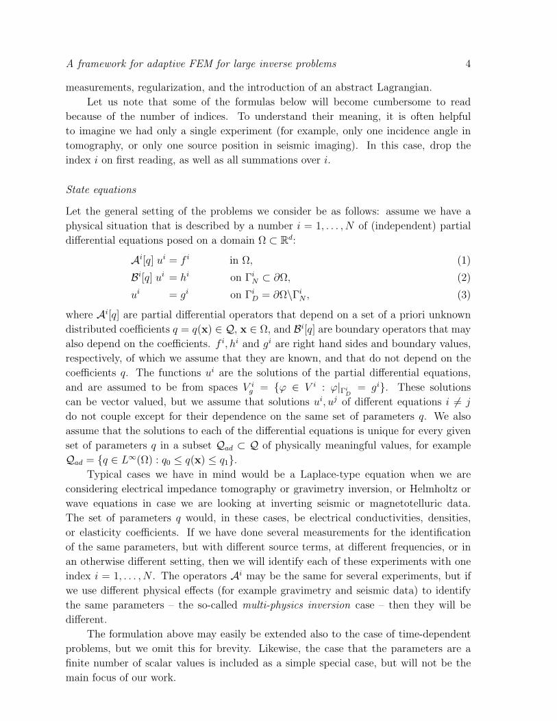
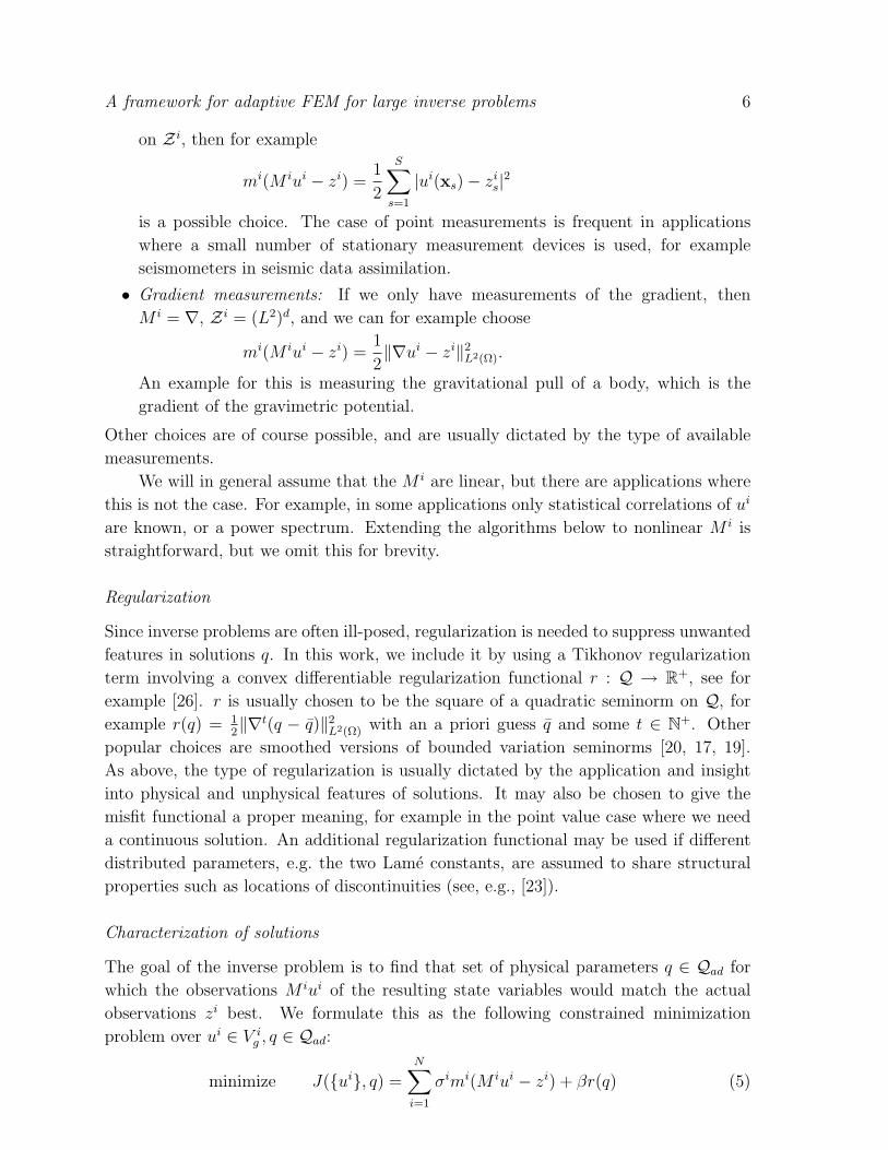
Figure 1. Example 1: Exact coefficient q∗ (left) and displacement u∗ (right).
Figure 2. Example 1: Recovered coefficient with no noise, on grids Tq with 800-900degrees of freedom. Left: No bounds on q imposed. Right: 1 ≤ q ≤ 8 imposed.
The coefficient q∗ we try to identify on a square domain is given by
q∗(x) =
1 for |x| < 1
2,
8 else.
Note that the circular jump in the coefficient is not aligned with the mesh cells, so
that we will need mesh refinement to resolve it properly. With f = 2d, d = dimΩ, the
solution of the Laplace equation is u∗(x) = |x|2 inside |x| < 12, and u∗(x) = 1
8|x|2 + 7
32
otherwise. u∗ and q∗ are shown in Figure 1. Measurement data is generated by choosing
z(x) = u∗(x) + ε(x), where ε is random noise with a fixed amplitude ‖ε‖∞.
For the case of no noise, i.e. measurements can be made everywhere without error,
Figure 2 shows the discretization grid for and the values of the identified parameter after
some refinement steps, at the left with no bounds on q imposed and at the right with
tight bounds 1 ≤ q ≤ 8. The latter case is typical if one knows that a body is composed
of two different materials, but their interface is unknown. In both cases, the accuracy
of reconstruction is good, and it is clear that adding bound information stabilizes the
process. No regularization is used for this experiment.
A framework for adaptive FEM for large inverse problems 22
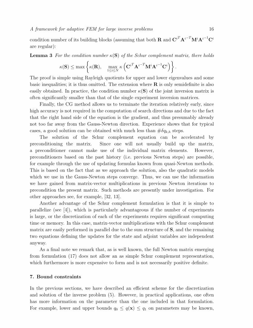
Figure 3. Example 1: Same as Fig. 2, but with 2% noise in the measurement.
On the other hand, if noise is present, Figure 3 shows the identified coefficient
without and with bounds on the parameter imposed. The noise level is ‖ε‖∞/‖z‖∞ ≈0.02. Again, no regularization is used, and it is obvious that the additional
information of bounds on the parameter improves the result significantly (quantitative
results are given as part of the next section). Of course, adding a regularization
term would also be a possible way to get a better reconstruction. However, since
devising regularization functionals for discontinuous coefficients is difficult and often
involves Bounded Variation-type seminorms with their well-known difficulties (see, e.g.,
[20, 17, 19]), we will not venture further in this direction and rather consider noise
suppression by multiple measurements in the next section.
8.2. Example 2: Multiple experiments
Let us consider the same situation as in the previous section, but this time use multiple
measurements zi of the data and for each measurement use a different forcing f i. Thus,
for each experiment 1 ≤ i ≤ N , we have
Ai(q;ui)(ϕ) = (q∇ui,∇ϕ)− (f i, ϕ), (27)
mi(M iui − zi) =1
2‖ui − zi‖2
Ω.
Our hope is that if each of these measurements is noisy, we can still recover the
correct coefficient well if we only measure often enough. Since the measurements have
independent noise, measuring more than once already yields a gain if the experimental
setup is identical, i.e. when the right hand sides f i are the same. However, simple
considerations indicate that q is not identifiable at points where ∇u∗ is zero, see for
example [8]; we thus gain more if we use different forcing functions f i (with different
sets of points where ∇ui = 0) in different experiments, and numerical studies also show
that this significantly increases the obtained accuracy, see [4].
In addition to the constant right hand side f 1(x) = 2d and matching boundary
conditions already used in the last section and shown in Fig. 1, we use as forcing terms

A framework for adaptive FEM for large inverse problems 23
Figure 4. Example 2: Solutions of the state equations for experiments i = 2, 6, 12.
Figure 5. Error ‖qh − q∗‖L2(Ω) in the reconstructed coefficient as a function of thenumber N of experiments used in the reconstruction and the average number of degreesof freedom used in the discretization of each experiment. Left: No bounds imposed.Right: 1 ≤ q ≤ 8 imposed. 2% noise in both cases. Note the different scales.
f i : Rd 7→ R, 2 ≤ i ≤ N for the different state equations (27) the functions
f i(x) = π2k2i sin(πki · x),
where the vectors ki are the first N elements of the integer lattice Nd =
(0, 0), (1, 0), (1, 1), (0, 1), ... when ordered by their l2-norm and after eliminating
collinear pairs in favor of the element of smaller magnitude. Numerical solutions for
these right hand sides are shown in Fig. 4 for i = 2, 6, 12. Measurements zi were
obtained by numerically solving the state equations with the exact coefficient using a
discretization of higher order than the one used in the reconstruction algorithm; random
noise was then added to this numerical solution.
Fig. 5 shows a quantitative comparison of the reconstruction error ‖qh − q∗‖L2(Ω),
as we increase the number of experiments used for the reconstruction, and as Newton
iterations proceed on successively finer grids. In most cases, we only perform one Newton
iteration on each grid, but if we are not satisfied with the progress on this grid, more
than one iteration will be done; in this case, curves in the charts have vertically stacked
data points, i.e. more than one data point for the same number of cells. The finest
discretizations had 3-400,000 degrees of freedom for the discretization of state and

A framework for adaptive FEM for large inverse problems 24
adjoint variable in each experiment (i.e., up to a total of about 4 million unknowns
in the examples shown), and about 10,000 degrees of freedom for the discretization
of the parameter qh; this then also was the size of the Schur complement matrix to be
solved in each step, which takes between 100 and 200 CG iterations to solve to a relative
accuracy of 10−3. We only show the case of non-zero noise level, since otherwise the
number of experiments was not relevant for the reconstruction error.
From the charts, it is obvious that imposing bounds helps significantly, and that
using more measurements is sufficient to strongly reduce the effects of noise. Also
note that if noise is present, there is a limit for the amount of information that can
be obtained and that further refining meshes deteriorates the result afterwards (see
the erratic and growing behavior of curves for small N for high number of degrees of
freedom; the identified parameter then deteriorates by high frequency oscillations). Since
the numerical effort required to solve the problem grows roughly linear with the number
of experiments, using more experiments may actually be cheaper in many cases, as the
discretization of each of them requires significantly less degrees of freedom to achieve a
given accuracy for the reconstructed parameter than if we used less experiments.
9. Conclusions and outlook
In this paper, we have presented a framework for the solution of large-scale multiple-
experiment inverse problems. It’s main features are:
• formulation in function spaces, allowing for different discretizations in subsequent
steps of Newton-type nonlinear solvers;
• discretization by adaptive finite element schemes, with different meshes for state
and adjoint variables on the one hand, and the parameters sought on the other;
• inclusion of bound constraints with a simple but efficient active set strategy;
• choice of a formulation that allows for efficient parallelization.
This framework has then been applied to some examples showing that inclusion of
bounds can stabilize the identification of a coefficient from noisy data, as well as the
(obvious) fact that measuring more than once can reduce the effects of noise. For these
numerical examples, only a rather simple criterion was used to drive mesh refinement.
The framework as laid out above will be used as the basis for further articles in this
series. In particular, while the entire framework is taylored to the use of different meshes,
we have not shown how to construct them in a systematic way. Thus, in the second part,
we will derive error estimates for the finite element discretization with respect to the
minimization functional J(u, q), i.e. estimates for the quantity J(u, q)− J(uh, qh), and
use them to drive adaptive mesh refinement. We will also discuss how to couple mesh
refinement strategies with the outer Newton-type iteration, and how to derive estimates
for arbitrary functionals of the solution. This allows to specify, for example, that we
are interested in the values of the coefficient only in part of the domain, and drive mesh
adaptivity for this particular goal. These techniques will again be demonstrated using

A framework for adaptive FEM for large inverse problems 25
numerical examples involving the identification of a coefficient from the solution of a
Laplace equation.
In a final part, all these techniques will be applied to wave propagation problems
involving the Helmholtz equation.
Acknowledgments. Part of this work has been done while at the Institute
of Applied Mathematics, University of Heidelberg; this work has been supported by
the Graduiertenkolleg “Modellierung und Wissenschaftliches Rechnen in Mathematik
und Naturwissenschaften”. Recent work on this project is financed by a Postdoctoral
Research Fellowship by the Institute for Computational Engineering and Sciences,
University of Texas at Austin. Support by both institutions is greatly acknowledged.
Computational resources have also been provided by the CFDlab at the University of
Texas at Austin.
The author would like to thank Rolf Rannacher for his support and encouragement
for this work.
Bibliography
[1] R. Acar. Identification of coefficients in elliptic equations. SIAM J. Control Optim., 31:1221–1244,1993.
[2] U. M. Ascher and E. Haber. Grid refinement and scaling for distributed parameter estimationproblems. Inverse Problems, 17:571–590, 2001.
[3] U. M. Ascher and E. Haber. A multigrid method for distributed parameter estimation problems.Technical report, University of British Columbia, 2002.
[4] W. Bangerth. Adaptive Finite Element Methods for the Identification of Distributed Coefficientsin Partial Differential Equations. PhD thesis, University of Heidelberg, 2002.
[5] W. Bangerth, R. Hartmann, and G. Kanschat. deal.II Differential Equations Analysis Library,Technical Reference, 2004. http://www.dealii.org/.
[6] W. Bangerth and G. Kanschat. Concepts for object-oriented finite element software – the deal.IIlibrary. Preprint 99-43, SFB 359, Universitat Heidelberg, October 1999.
[7] W. Bangerth and R. Rannacher. Adaptive Finite Element Methods for Differential Equations.Birkhauser Verlag, 2003.
[8] H. T. Banks and K. Kunisch. Estimation Techniques for Distributed Parameter Systems.Birkhauser, Basel–Boston–Berlin, 1989.
[9] R. Becker. Adaptive finite elements for optimal control problems. Habilitation thesis, Universityof Heidelberg, 2001.
[10] R. Becker, H. Kapp, and R. Rannacher. Adaptive finite element methods for optimal control ofpartial differential equations: Basic concept. SIAM J. Contr. Optim., 39:113–132, 2000.
[11] R. Becker and B. Vexler. Mesh adaptation for parameter identification problems. Proceedings ofENUMATH 2001, 2002. submitted.
[12] M. Bergounioux, K. Ito, and K. Kunisch. Primal-dual strategy for constrained optimal controlproblems. SIAM J. Control Optim., 37:1176–1194, 1999.
[13] G. Biros and O. Ghattas. Parallel Lagrange-Newton-Krylov-Schur methods for PDE-constrainedoptimizaion. Part I: The Krylov-Schur solver. submitted, 2003.
[14] A. Bjorck. Numerical Methods for Least Squares Problems. SIAM, 1996.[15] H. G. Bock. Randwertproblemmethoden zur Parameteridentifizierung in Systemen nichtlinearer
Differentialgleichungen, volume 183 of Bonner Mathematische Schriften. University of Bonn,Bonn, 1987.
[16] J. Carter and C. Romero. Using genetic algorithms to invert numerical simulations. In ECMOR

A framework for adaptive FEM for large inverse problems 26
VIII: 8th European Conference on the Mathematics of Oil Recovery, Freiberg, Germany, pagesE–45. European Association of Geoscientists and Engineers (EAGE), 2002.
[17] Z. Chen and J. Zou. An augmented Lagrangian method for identifying discontinuous parametersin elliptic systems. SIAM J. Control Optim., 37:892–910, 1999.
[18] M. J. Dayde, J.-Y. L’Excellent, and N. I. M. Gould. Element-by-element preconditioners for largepartially separable optimization problems. SIAM J. Sci. Comp., 18:1767–1787, 1997.
[19] F. Dibos and G. Koepfler. Global total variation minimization. SIAM J. Numer. Anal., 37:646–664, 2000.
[20] S. Gutman. Identification of discontinuous parameters in flow equations. SIAM J. ControlOptimization, 28(5):1049–1060, 1990.
[21] E. Haber and U. M. Ascher. Preconditioned all-at-once methods for large, sparse parameterestimation problems. Inverse Problems, 17:1847–1864, 2001.
[22] E. Haber, U. M. Ascher, and D. Oldenburg. On optimization techniques for solving nonlinearinverse problems. Inverse Problems, 16:1263–1280, 2000.
[23] E. Haber and D. Oldenburg. Joint inversion: a structural approach. Inverse Problems, 13:63–77,1997.
[24] K. Ito, M. Kroller, and K. Kunisch. A numerical study of an augmented Lagrangian method forthe estimation of parameters in elliptic systems. SIAM J. Sci. Stat. Comput., 12:884–910, 1991.
[25] D. W. Kelly, J. P. de S. R. Gago, O. C. Zienkiewicz, and I. Babuska. A posteriori error analysisand adaptive processes in the finite element method: Part I–error analysis. Int. J. Num. Meth.Engrg., 19:1593–1619, 1983.
[26] C. Kravaris and J. H. Seinfeld. Identification of parameters in distributed parameter systems byregularization. SIAM J. Control Optim., 23:217–241, 1985.
[27] R. Li, W. Liu, H. Ma, and T. Tang. Adaptive finite element approximation for distributed ellipticoptimal control problems. SIAM J. Control Optim., 41:1321–1349, 2002.
[28] R. Luce and S. Perez. Parameter identification for an elliptic partial differential equation withdistributed noisy data. Inverse Problems, 15:291–307, 1999.
[29] X.-Q. Ma. A constrained global inversion method using an over-parameterised scheme: Applicationto poststack seismic data. Geophysics Online, August 2000.
[30] J. Nocedal and S. J. Wright. Numerical Optimization. Springer Series in Operations Research.Springer, New York, 1999.
[31] M. K. Sen, A. Datta-Gupta, P. L. Stoffa, L. W. Lake, and G. A. Pope. Stochastic reservoirmodeling using simulated annealing and genetic algorithms. SPE Formation Evaluation, pages49–55, March 1995.
[32] C. R. Vogel. Sparse matrix computations arising in distributed parameter identification. SIAMJ. Matrix Anal. Appl., 20:1027–1037, 1999.
[33] C. R. Vogel. Computational Methods for Inverse Problems. SIAM, 2002.[34] W. H. Yu. Necessary conditions for optimality in the identification of elliptic systems with
parameter constraints. J. Optimization Theory Appl., 88:725–742, 1996.


