dove or hawk? characterizing monetary policy regime ...boxjenk/1-s2.0-s1566014113000411-main.pdf ·...

Emerging Markets Review 16 (2013) 183–202

Contents lists available at SciVerse ScienceDirect

Emerging Markets Review

j ourna l homepage: www.e lsev ie r .com/ locate /emr

Dove or Hawk? Characterizing monetary policy
regime switches in India☆
Michael M. Hutchison a,⁎, Rajeswari Sengupta b, Nirvikar Singh a

a University of California, Santa Cruz, USAb Institute for Financial Management and Research, Chennai, India

a r t i c l e i n f o

☆ We are grateful to the editor of this journal, particNew Delhi, especially our discussant Ila Patnaik, and⁎ Corresponding author at: Department of Econom

E-mail address: [email protected] (M.M. Hutchison

1566-0141/$ – see front matter © 2013 Elsevier B.V.http://dx.doi.org/10.1016/j.ememar.2013.05.005

a b s t r a c t

Article history:Received 7 March 2013Received in revised form 15 May 2013Accepted 16 May 2013Available online 25 May 2013

The past two decades have witnessed a worldwide move by emergingmarkets to adopt explicit or implicit inflation targeting regimes. Anotable and often discussed exception to this trend, of course, is Chinawhich follows a pegged exchange rate regime supported by capitalcontrols. Another major exception is India. It is not clear how tocharacterize the monetary regime or identify the nominal monetaryanchor in India. Is central bank policy in India following a predictablerule that is heavily influenced by a quasi inflation target? And how hasthe monetary regime been affected by the gradual process of financialliberalization in India? To address these points,we investigatemonetarypolicy regime change in India using a Markov switching model toestimate a time-varying Taylor-type rule for the Reserve Bank of India.We find that the conduct of monetary policy over the last two decadescan be characterized by two regimes, which we term ‘Hawk’ and ‘Dove.’In the first of these two regimes, the central bank reveals a greaterrelative (though not absolute) weight on controlling inflation vis-à-visnarrowing the output gap. The central bank howeverwas found to be inthe “Dove” regime about half of our sample period, focusingmore on theoutput gap and exchange rate targets to stimulate exports, rather thanmoderating inflation. India thus seems to be following its own directionin the conduct of monetary policy, seemingly not overly influenced bythe emphasis on quasi-inflation targeting seen in many emergingmarkets.

© 2013 Elsevier B.V. All rights reserved.

JEL classification:E4E5F3F4

Keywords:Monetary policyTaylor ruleMarkov regime switchingInflation targetingRBI's discretionary policy

ipants at the 6th NIPFP-DEA research programmeeting onMarch 9–10, 2010 inDeepak Mohanty for helpful comments.ics, E2, University of California Santa Cruz, Santa Cruz, CA 95064, USA.).

All rights reserved.

http://crossmark.dyndns.org/dialog/?doi=10.1016/j.ememar.2013.05.005&domain=pdf

http://dx.doi.org/10.1016/j.ememar.2013.05.005

mailto:[email protected]

http://dx.doi.org/10.1016/j.ememar.2013.05.005

http://www.sciencedirect.com/science/journal/15660141

184 M.M. Hutchison et al. / Emerging Markets Review 16 (2013) 183–202

1. Introduction

Amajor switch in the conduct ofmonetary policy has occurred inmany nations over the past two decades.Although taking different forms, the switch has been towardsmore systematic rules and less discretion in theconduct of monetary policy. Many central banks in emerging markets have adopted formal inflation targets(ITs), includingBrazil, Chile, Colombia, CzechRepublic, Korea, Hungary, Israel, Peru, Philippines, Poland, SouthAfrica, Thailand and Turkey. Other central banks have adopted systematic rules that de facto describe thebehavior of the central bank's operating instrument response—usually interbank interest rates—to inflation,output gaps and the external environment. Rose (2007) argues that the move to IT regimes, either explicitlyor implicitly (e.g. adopting systemic rules focusing on inflation), has created a new monetary system that ismore stable than its predecessors such as exchange rate targeting and fixed exchange rates that existed in theerstwhile Bretton Woods system.

Theoretical studies that derive optimal monetary policy rules, and empirical studies that investigate theiruse in practice, are now commonplace in the literature (e.g. Taylor, 1993; Clarida et al., 2000;Woodford, 1999,2001; Giannoni and Woodford, 2002). Taylor (1993) formulated a policy rule by which the U.S. FederalReserve adjusts the policy rate in response to past inflation and the output gap (actual less potential output).He showed that this rule described Federal Reserve policy performance quite well from 1987 to 1992. Using aquadratic loss function for the welfare objective of the central bank, Woodford (2001) provided a formalnormative justification for following a Taylor-type rule under certain conditions. Many studies subsequentlyapplied and developed this class of policy rules to examine the behavior of central banks in industrializedcountries (e.g., Clarida et al., 2000), and several have been applied to emerging and developing economies(e.g. Aizenman et al., 2011; Gonçalves and Salles, 2008). In fact, Gonçalves and Salles (2008) find that in asample of 36 emerging market economies (13 of which implemented IT), the IT adopters experienced agreater decline in inflation and growth volatility compared to the non-adopters.

In light of the 2008–09 global financial crisis, it may be premature to make a final judgment on thedesirability and durability of IT regimes andwhether theirwidespread adoption has actually ushered in a newera of global monetary stability. It is noteworthy that the two largest, most populous, and, arguably, dynamicemerging markets, China and India, have not adopted IT regimes and withstood the global financial crisisreasonably well. China follows a quasi-fixed exchange rate regime against the U.S. Dollar, accumulatesmassive international reserves and maintains tight capital controls to keep the parity unchanged (e.g. Glickand Hutchison, 2009; Ouyang et al., 2010). In contrast, themonetary policy regime in India is less explicit andapparently more dynamic, with the authorities typically arguing that discretion is paramount in their policydecisions. 1

The objective of our paper is to investigate the nature of monetary policy rules in India, a country that hasundergone substantial domestic financial development and deregulation over the past two decades and hasalso experienced significant integration with the global economy. These developments have potentiallyaltered the financial environment and external constraints (e.g. balance of payments, exchange rates) facingthe central bank (Reserve Bank of India, RBI), andmay have influenced its operating procedures as well as itspolicy tradeoffs between output–inflation–exchange rate stabilization. These considerations, in turn, mayhave impacted the formulation ofmonetary policy rule in India asmentioned inMohan (2006b). In particular,moneymarket deregulation took place in 1987. Prior to that, themoneymarket was highly regulated and theinterest rate was essentially fixed.2 Since 1987 there has beenmuch greater flexibility inmoneymarket rates,and the RBI started using it as the primary operating instrument of monetary policy. To this end, weinvestigate the monetary policy rule in India and whether simple Taylor-like policy rules—perhaps changingover time to account for the changing economic environment—may be employed to systematically describeRBI's actions. The RBI describes its own policy actions in terms of discretion, and states that a multitude offactors are taken into considerationwhen deciding the course ofmonetary policy. The question iswhether theseemingly discretionary policy followed by the RBI may be empirically described by a systemic rule thatallows for occasional regime switches.

1 India and China are included in the Gonçalves and Salles (2008) sample as non-IT adopters.2 While arguments can be made for later starting dates, given the evolution of financial liberalization in India, and of the RBI's

conduct of monetary policy, this particular liberalization episode seems to be the most appropriate beginning for our sample period.

185M.M. Hutchison et al. / Emerging Markets Review 16 (2013) 183–202

Thus, our paper focuses on the monetary policy rule followed in India. In doing so, our analysis contributesto the relevant literature by adopting a regime switchingmodel along the lines of Hamilton (1989) to allow formultiple changes over time in central bank preferences between “Hawk” and “Dove”monetary regimes that, inturn, shift the central bank operating policy rule. Previous work for emerging markets has focused on a stablemonetary policy rule (constant coefficients) over time or perhaps a discrete shift from one rule to another inlinewith a change in the central bank leadership, institutional change or political change.3 None has focused onmonetary regime switching either in emerging market economies in general or in India in particular. Ourapproach, by contrast, allows for the Indian central bank to operate in either of two regimes, and switch fromone regime to another, multiple times in response to changes in the macro-economic conditions (e.g. inflationrate, output gap, and the exchange rate). For example, at times the RBI may be primarily concerned withinflation in a “Hawk” regime, perhaps because inflation is viewed as the primary threat to economic stability,while at other times its focus may be shifted to stimulating output (“Dove” regime). These shifts may occurpredictably over the business cycle or at other times, not necessarily representing an institutional change, butsimply a complex policy rule that changes over time, shiftingwith a given probability in response to an evolvingeconomic environment.

Our application of the regime-switching model to Indian monetary policy is interesting in its own right.Much like the U.S. Federal Reserve, the RBI has seemingly responded to the state of the economy in anapparently discretionary and flexiblemanner. A former Deputy Governor of the RBI described their approach asfollows, “Thus the overall objective has had to be approached in a flexible and time variant manner with acontinuous rebalancing of priority between growth and price stability, depending on underlying macroeconomicandfinancial conditions.” (Mohan, 2006a; italics our own). The question iswhether the apparently discretionaryandflexible approach of the RBI can systematically and empirically be described in practice by a Taylor-type rule,albeit with the possibility of regime switches. Based on description of the conduct of monetary policy by RBIofficials, India appears to be a good candidate to be described by a regime switching model between Hawk andDove regimes.

No study to date has undertaken this line of research for India. In particular, only three studies that we areaware of have investigatedmonetary policy rules for India, none of which have considered regime-switching.In particular, Mohanty and Klau (2005) augment the Taylor rule to include changes in the real effectiveexchange rate. They use quarterly data from 1995 to 2002 for 13 emerging economies including India. Theyfind that for India, the estimated inflation coefficient is relatively low whereas the output gap and realexchange rate change are significant determinants of the short-term interest rate. Virmani (2004) estimatesmonetary policy reaction functions for the Indian economy, with themonetary base (termed in the literatureas the McCallum Rule) and interest rate (Taylor Rule) as alternative operating targets.4 He finds that abackward-lookingMcCallum rule tracks the evolution of themonetary base over the sample period (1992q3–2001q4) reasonably well, suggesting that the RBI acts as if it is targeting nominal income when conductingmonetary policy. In addition, neither of these studies explores the Indian central bank's policy rule beyond theearly 2000s. Finally, Hutchison et al. (2010) estimate monetary policy rules for India with more recent databut use structural breaks chosen a priori as opposed to model-based estimates of systemic regime switches.5

In the next section we discuss the evolution of monetary policy in India and related literature. Wesummarize some of the major changes that took place in this sphere. In the third section we explain themethodology and data used.We describeWoodford's version of the Taylor Rule, andhowwe adaptHamilton'sMarkov switchingmethod to the case ofmonetary policy rules. In the fourth sectionwe present the estimationresults. In particular, the Markov switching model identifies two distinct regimes, which we label ‘Hawk’ and

3 Owyang and Ramey (2004), Assenmacher-Wesche (2005) and Frommel et al. (2005) consider regime-switching models formonetary policy rules for advanced economies. Liu (2010) considers regime-switching models for 17 IT-targeting countries (notincluding India). In an unpublished manuscript, Steiner et al. (2013) consider a Markov switching model for Chile and Colombiasince adopting an IT regime.

4 Other recent studies of India not using our methodology, are those of Singh (2010), Patra and Kapur (2012) and Mohanty(2013b). Studies that have used McCallum's rule of monetary policy for other countries include Burdekin and Siklos (2008).

5 In more general analyses of macro policy and financial structure, Hutchison et al. (2012a, 2012b) consider the trilemma trade-offfor India, focusing on the constraints on monetary policy imposed by the exchange rate regime and international capital controls.Hutchison et al. (2012a, 2012b) consider the extent to which financial liberalization in India has led to closer integration of domesticand international financial markets.


‘Dove.’ We begin with a model that focuses on domestic variables, and subsequently consider the role ofexchange rate in monetary policy making following Taylor (2001). In the fifth section we conclude bysummarizing our results and interpretation.

2. Monetary policy and financial liberalization in India

The Indian economy experienced several major structural changes in financial markets and fiscalfinancing over the sample period thatmay have potentially influenced the conduct ofmonetary policy. As hasbeen highlighted in debates about the timing of Indian economic reform (Panagariya, 2008), there was nosingle “big bang”moment, especiallywith respect to the evolution of thefinancial sector, making it difficult toidentify well-defined structural breaks in the Indian economy. Nonetheless, a number of key developmentsfor monetary policy may be identified. Firstly, fiscal deficits are no longer automatically parked with publicsector banks, neither are they passively monetized by the RBI (Shah, 2008). Secondly, the liberalization offinancial markets began in the late 1980s, moving towards a deeper financial sector and away from extremefinancial repression (Shah, 2008). The process of financial liberalization accelerated following the balance ofpayment crisis in 1991.

Between 1991 and 1997, lending rates of commercial banks were deregulated, the issue of ad hoctreasury bills was phased out (thereby eliminating automatic monetization of the budget deficit), StatutoryLiquidity Ratio (SLR) and Cash Reserve Ratio (CRR) rates were sharply reduced, and the RBI reactivated therefinance rate or bank rate (which is now used as a signaling rate to reflect the monetary policy stance). In1994, India switched over to a mainly market-determined exchange rate system and instituted currentaccount convertibility.

The RBI appears to have loosely targeted monetary growth between 1980 and 1998 and, from thenonwards, followed a multiple indicator approach with discretion. Starting in 1998, the RBI undertookstrong monetary policy measures (increasing interest rates and withdrawing liquidity by raising the CRR)to combat concerns about excessive liquidity and speculation in the foreign exchange market. The foreignexchange market was characterized by a high degree of volatility following the onset of the Asian financialcrisis towards the end of 1997 and beginning of 1998. These emergency measures were gradually reversedonce the threat of the crisis spilling over to India seemed to have abated.

The subsequent period, through the mid-2000s, saw the RBI continuing to refine its approach tomacroeconomic management. With global and domestic inflation at relatively low levels, the RBI set a bandfor target inflation of 4–5%, whichwas low by historical standards. It announced an intention to bring the CRRdown, and moved away from using the CRR as a policy instrument, focusing on interest rates instead—thisintention however was not realized, in practice. The RBI also continued to slowly ease capital controls, withimplications for the functioning of domestic financial markets. Relaxations of capital controls included easingof requirements for and caps on foreign institutional investors (FIIs), streamlining of approval processes, andallowing FIIs to hedge exchange rate risk in currency forwardmarkets. While domestic fixed incomemarketscontinued to be thin (as opposed to vibrant stock exchanges), especially for corporate bonds, a market forgovernment securities did develop during this period.

A significant development during this period was an institutional innovation introduced by the RBI tomanage its own open-market operations. The new institution, termed the Liquidity Adjustment Facility(LAF) was introduced on June 5, 2000. It operated through repo and reverse repo auctions, thereby settinga corridor for the short-term interest rates, consistent with the policy objectives. Thus, the LAF finally gavethe RBI an explicit method for monitoring short-term liquidity under varied financial market conditions, inorder to influence call money rates.

A final aspect of changingmonetarymanagementwas the increase in capital inflows that began in the lastdecade. Capital inflows, if unchecked, increase domestic money supply, resulting in a looser monetary policythan would otherwise be the case. Capital inflows also put pressure on the exchange rate to appreciate. TheRBI engaged in sterilization of inflows and accumulation of foreign exchange reserves in this time frame. TheRBI apparently had to deal with the trilemma of maintaining an independent monetary policy and stableexchange rate in the face of international capital flows. Accordingly, in this paper we address internationalfactors manifested through exchange rate fluctuations and empirically analyze the implications thereof onthe conduct of monetary policy in India.


This brief institutional discussion suggests that a regime-switching Taylor rule may be appropriate touncover the underlying preferences of the RBI's decision-makers and in particular, their evolution overtime. Given the seemingly discretionary nature of policy, as articulated in RBI statements, the central bank'srevealed preferences may be well captured by a model of systematic, though time-varying, behavioralresponses.

3. Methodology and data

3.1. Theory and estimation

The Woodford (2001) version of the Taylor Rule for an open economy expresses the policy instrument—the interbank interest rate—as a function of the output gap, inflation target, exchange rate and laggedinterest rate. With constant coefficients, this policy rule may be written as:

6 Unlmoneta

7 Asdifferenmaker c

it ¼ cþ αyt þ βπt þ χΔet þ δit−1 þ εt ð1Þ

where it is the nominal interest rate, yt is the output gap at time t (deviation of actual output, measured bythe index of industrial production, from potential output), πt is the year-on-year inflation rate (assuming aconstant inflation target such that the target is subsumed in the constant term of the equation) and etdenotes the log of exchange rate with Δ being the first difference operator.6 The expected signs of theestimated coefficients are: α, β,χ and δ > 0. The rule indicates a relatively high interest ratewhen inflation isabove its target, when the output is above its potential level, or when the central bank is attempting to limitexchange rate depreciation. The lagged interest rate is introduced to capture inertia in optimal monetarypolicy, as specified by Woodford (2001). We use end of period quarterly data for all variables for the period1987Q1–2008Q4.

Eq. (1) is the standard model for the estimation of central bank policy functions—assumes that thepolicy response to economic variables is stable over time. Some authors allow for a discrete shift in policyfollowing a central bank reform or other institutional change. Our argument above however, suggests thata central bank's preferences may change in a systematic and predictable manner such that there areswitches between periods when inflation is the primary concern of policy (“Hawk” regime) and when theoutput gap is the primary concern of policy (“Dove” regime). The distinction between Hawk and Doveregimes is common in the literature (see Assenmacher-Wesche, 2005; Owyang and Ramey, 2004, forrecent references). This implies that a regime-switching model that allows the coefficients to shiftbetween two states (s = 1, 2) would be a better representation of monetary policy than the alternative ofa one-regime (constant coefficients) model.7 In this circumstance, our estimation equation becomes:

it ¼ cþ αstyt þ βstπt þ χΔet þ δit−1 þ εt ð2Þ

with St representing the state at time t, i.e. St = 1 … k, where k is the number of states. Since we considerthe switching to take place between 2 states (“Hawk” and “Dove” regimes), k = 2 in our case. In additionto switching the coefficients, we also allow the variance of the error term to switch simultaneouslybetween the states, εt∼N 0;σ2

st� �

Markov switching models (MSMs), originally motivated by Goldfeld and Quandt (1973), have beenpopularized in business cycle and exchange rate analysis byHamilton (1989) and Engel andHamilton (1990).In our case, themodel allows us to estimate howmuchweight the RBI assigns to the relevantmacroeconomicvariables in two different regimes. In aMSM, switching between regimes does not occur deterministically butwith a certain probability. In general terms, the evolution of the discrete, unobserved state-variable St isserially dependent upon St − 1, St − 2,… St − r, in which case the process is referred to as an rth order Markovswitching process.

ike the central banks of developed countries, the RBI does not have a forward-looking approach when it comes to decidingry policy.noted earlier, one can allow for structural breaks in estimation, but the regime-switching method allows for a somewhatt approach to changing policy responses — the maintained hypothesis is of two policy stances, between which the policyhooses, depending on economic conditions.


As noted above, we assume a two-state, first order Markov switching process for St, characterized byconstant transition probabilities pij = Pr{St = m|St − 1 = n}. In particular, let P denote the 2 × 2 transitionprobability matrix for our two-state Markov process such that:

whereto as tterms

whereabovediscus

whereSt = m

8 Eq.or anotperiod t

9 ThePerlin (10 We

P ¼ p11 p21p12 p22

� �: ð3Þ

The estimation procedure classifies each observation as belonging to either regime. The regimes however,are not observed or specified ex-ante, but are estimated from the data.

To estimate the model, we consider the joint distribution of it and St conditional on past information:

f it ; Stð jψt−1Þ ¼ f itð jSt ;ψt−1Þf Stð jψt−1Þ ð4Þ

where Ψt − 1 denotes information at time t − 1 and f(it|St, Ψt − 1) is the conditional normal densityfunction for the regime St = m. The likelihood function we estimate is a weighted average of the densityfunctions for the two regimes, the weights being the probability of each regime:

lnL ¼XTt¼1

lnX2m¼1

f itð jSt ;ψt−1ÞPr St ¼ mð jψt−1Þ( )

ð5Þ

the weighting term Pr(St = m|ψt − 1) is the probability of being in each regime and is also referredhe filtered probability. Given Pr(St − 1 = n|ψt − 1), n = 1,2, at the beginning of time t the weightingPr(St = m|Ψt − 1) are calculated as:

Pr St ¼ mð jψt−1Þ ¼X2n¼1

Pr St ¼ m St−1 ¼ nj ÞPr St−1 ¼ nð jψt−1ð Þ ð6Þ

Pr(St = m|St − 1 = n), m = 1, 2; n = 1, 2, are the transition probabilities (elements of matrix P).8 OnceΨt is observed at the end of time t, the probabilities are updated using the iterative filter, assed in Kim and Nelson (1999). The updated probabilities are calculated as follows:

Pr St ¼ mð jψtÞ ¼f itð jSt ¼ m;ψt−1ÞPr St ¼ mð jψt−1ÞX2

m¼1

f itð jSt ¼ m;ψt−1ÞPr St ¼ mð jψt−1Þð7Þ

f(it|St = m, ψt − 1) is given by the probability density function of a normal distribution for regime. Note that this is simply Bayesian updating of the probabilities of being in each state, given theation available then.
inform
To start thefilter at time t = 1,weuse the initial values obtained fromanordinary least squares regression.Once the coefficients of the model are estimated using an iterative maximum likelihood procedure and thetransition probabilities are generated,we canuse the algorithm inKimandNelson (1999) to derive thefilteredprobabilities for St using all the information up to time t i.e. Pr(St = m|ψT) where t = 1, 2, …, T.9

3.2. Data

For the short-term policy rate, we use the overnight call money market rate.10 This is the standardinterest rate used to indicate the policy stance of the central bank. The RBI follows a multiple instrument

(6) is useful in showing that while the transition probabilities are constant, the conditional probability of being in one regimeher depends on the history of the economy, summarized in the information available at that time, and therefore varies fromo period.MSMmodel is estimated using the MS-Regress Matlab package for Markov Regime Switching Models, developed by Marcelo2009).use the call money market rate primarily because of availability of consistent data during our sample period.

Fig. 1. Output gap and inflation (WPI).


approach to influence the call money rate. An important issue, especially in India, is the measurement of theoutput gap. Unlike advanced countries, there are no official measures of potential output levels. Virmani(2004) compared estimated potential GDP obtained from an unobserved component model with estimatesderived from a Hodrick–Prescott (HP) filter, and found little difference. Accordingly we derive the output gapusing theHPfilter formeasuring trend output and taking the residual of theHPfilter.11 Tomeasure output, weuse the Index of Industrial Production (IIP).12 Year-on-year inflation is measured using annual percentagechange in the Wholesale Price Index (WPI). The WPI is the price level employed by the RBI to calculate“headline” inflation in India. All data are quarterly and the overall sample period is 1987q1 to 2008q4. Westart our sample at 1987q1 because interest rate regulation essentially fixed the money market rate prior tothat time.With broad changes in the financial system in the late 1980s, camemoneymarket deregulation andat that time themoneymarket rate became the primary operating instrument of the RBI. We stop our sampleat the beginning of the transmission of the global financial crisis to India, as there was a distinct disruption indomestic financial markets at that time, and policy shifted away from traditional monetary policy operations.

Prior to estimation, several data issues were dealt with. Analysis of linear plots and the Hylleberg–Engle–Granger–Yoo test suggest that the quarterly IIP series has multiplicative seasonality. Hence it wasde-seasonalized using the X-12 ARIMA procedure. Unit root tests, i.e. Augmented Dickey–Fuller, Phillips–Perron, Elliott–Rothenberg–Stock and Kwiatkowski–Phillips–Schmidt–Shin test results suggest the presenceof unit root in the exchange rate series in levels, but the first difference of the series is stationary. Accordingly,thefirst difference of the nominal exchange ratewas used. DurbinWatson and Breusch–Godfrey tests suggestthe presence of serial correlation and the Breusch–Pagan/Cook–Weisberg test shows the presence ofheteroskedasticity in error terms. Hence the Ordinary Least Squares (OLS) regressions have been runwith theNewey–West variance–covariance matrix, to correct for both autocorrelation and heteroskedasticity.

Finally,we discuss our treatment of the interest rate series. Someother studies have used an average of theinterest rate over the preceding quarter (or whatever the length of the period), presumably to capture theaverage policy stance for that period. However, this is not completely logical, since it creates a dependentvariable that is partially determined prior to the right-hand side observations. Using the end-of-quarterinterest rate avoids this inconsistency.

11 The HP filter output is sensitive to the endpoints, and we examine the robustness of our results to this issue: this point is takenup in the Empirical results section.12 We also estimated output gap using real GDP (from 1994 onwards, conditional on data availability) and the results were foundto be quite similar.

Fig. 2. Interest rate and inflation (WPI).


4. Empirical results

4.1. Preliminaries

Figs. 1–3 show movements between the output gap and inflation (Fig. 1), interest rate and inflation(Fig. 2), and interest rate and output gap (Fig. 3) in India over the 1987q1 to 2008q4 period. Table 1 showsthe corresponding correlations between these series for the full sample (1987–2008), early sample(1987–1995) and later sample (1996–2008).

Fig. 1 does not show a distinct pattern between the output gap (right-hand-side scale) and inflation(left-hand-side scale) during the full sample period (overall correlation = −0.02), although a weakpositive (and statistically significant) correlation emerges in the later period (0.06). The “output–inflationtradeoff” is not clearly evident through simple co-movements in these variables, but the relationship maybe masked by a variety of real and financial disturbances to the Indian economy as well as by an activistmonetary policy.

Fig. 2 shows the evolution of the interest rate (i.e. the overnight money market rate) and inflation.Trend inflation seems to have declined in India over the sample period. Inflation averaged at about 9%,

Fig. 3. Interest rate and the output gap.

image of Fig.�2

image of Fig.�3

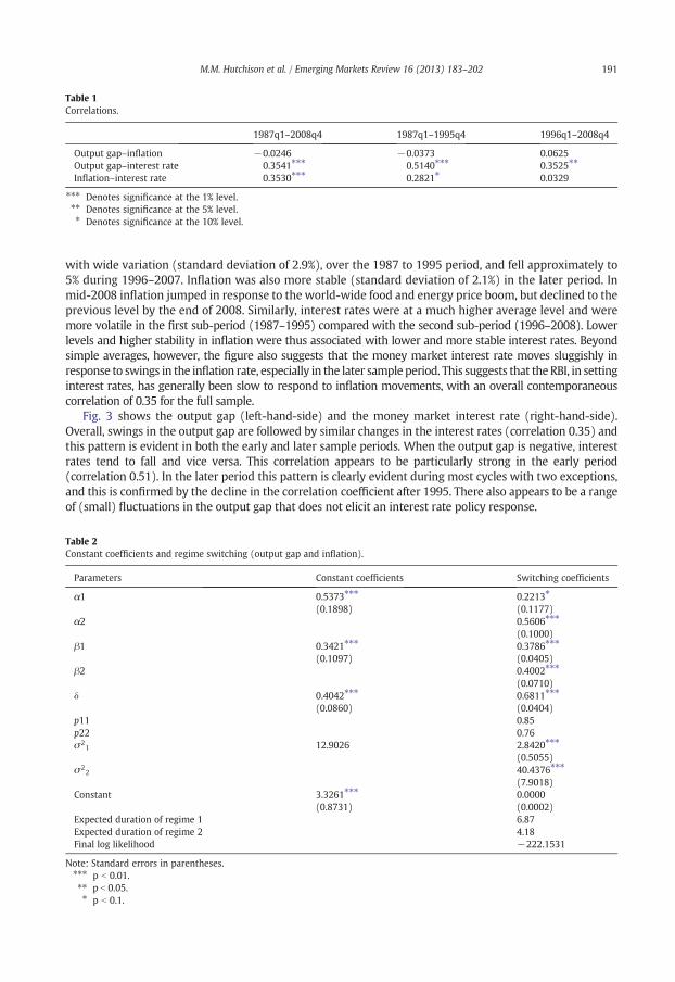
Table 1Correlations.

1987q1–2008q4 1987q1–1995q4 1996q1–2008q4

Output gap–inflation −0.0246 −0.0373 0.0625Output gap–interest rate 0.3541⁎⁎⁎ 0.5140⁎⁎⁎ 0.3525⁎⁎

Inflation–interest rate 0.3530⁎⁎⁎ 0.2821⁎ 0.0329

⁎⁎⁎ Denotes significance at the 1% level.⁎⁎ Denotes significance at the 5% level.⁎ Denotes significance at the 10% level.


with wide variation (standard deviation of 2.9%), over the 1987 to 1995 period, and fell approximately to5% during 1996–2007. Inflation was also more stable (standard deviation of 2.1%) in the later period. Inmid-2008 inflation jumped in response to the world-wide food and energy price boom, but declined to theprevious level by the end of 2008. Similarly, interest rates were at a much higher average level and weremore volatile in the first sub-period (1987–1995) compared with the second sub-period (1996–2008). Lowerlevels and higher stability in inflation were thus associated with lower and more stable interest rates. Beyondsimple averages, however, the figure also suggests that the money market interest rate moves sluggishly inresponse to swings in the inflation rate, especially in the later sample period. This suggests that the RBI, in settinginterest rates, has generally been slow to respond to inflation movements, with an overall contemporaneouscorrelation of 0.35 for the full sample.

Fig. 3 shows the output gap (left-hand-side) and the money market interest rate (right-hand-side).Overall, swings in the output gap are followed by similar changes in the interest rates (correlation 0.35) andthis pattern is evident in both the early and later sample periods. When the output gap is negative, interestrates tend to fall and vice versa. This correlation appears to be particularly strong in the early period(correlation 0.51). In the later period this pattern is clearly evident during most cycles with two exceptions,and this is confirmed by the decline in the correlation coefficient after 1995. There also appears to be a rangeof (small) fluctuations in the output gap that does not elicit an interest rate policy response.

Table 2Constant coefficients and regime switching (output gap and inflation).

Parameters Constant coefficients Switching coefficients

α1 0.5373⁎⁎⁎

(0.1898)0.2213⁎

(0.1177)α2 0.5606⁎⁎⁎

(0.1000)β1 0.3421⁎⁎⁎

(0.1097)0.3786⁎⁎⁎

(0.0405)β2 0.4002⁎⁎⁎

(0.0710)δ 0.4042⁎⁎⁎

(0.0860)0.6811⁎⁎⁎

(0.0404)p11 0.85p22 0.76σ2

1 12.9026 2.8420⁎⁎⁎

(0.5055)σ2

2 40.4376⁎⁎⁎

(7.9018)Constant 3.3261⁎⁎⁎

(0.8731)0.0000(0.0002)

Expected duration of regime 1 6.87Expected duration of regime 2 4.18Final log likelihood −222.1531

Note: Standard errors in parentheses.⁎⁎⁎ p b 0.01.⁎⁎ p b 0.05.⁎ p b 0.1.


In sum, it appears that the RBI responds both to the output gap and inflation in setting policy interestrates. Interestingly, the correlations for both output gap and inflation with moneymarket interest rates arealmost identical over the full sample period (0.35) and both correlations decline after 1995, especially thecontemporaneous linkage between interest rates and inflation.

Another variable that the RBI may sometimes target is the exchange rate. The RBI itself has argued thatits focus has only been on controlling the volatility of exchange rate movements, rather than targeting thelevel of exchange rate. However, some analyses (e.g., Patnaik, 2007) have suggested that at times there hasbeen a systematic attempt by the RBI to manage the level of the nominal Rupee–Dollar rate. In order toaddress this issue, we extend the basic Taylor Rule model to one that also includes the exchange rate as adeterminant of policy, as shown in Eq. (1).

4.2. Constant coefficient estimates

Thefirst columnof coefficient estimates in Table 2 presents the results fromestimating Eq. (1) i.e. assumingconstant coefficients, but with the exchange rate omitted. The coefficients on the output gap, inflation andlagged interest rate are all significant at the 1% level and have signs predicted by theory. These estimatessuggest that the RBI increases the overnight interest rate by 54 basis points in response to a one unit rise in theoutput gap (where positive increases in the output gap represent a rise in output relative to trend). The RBIalso increases the interest rate by 33 basis points in response to a 100 basis point rise in inflation. The laggedinterest rate coefficient of 0.40 suggests considerable inertia in policy implying that the long-run effects aresubstantially greater than the short-run impact effects. The long-run effect on the interest rate of a unit changein the output gap is 0.89 and of a 100 basis point increase in inflation is 0.55. The 95% confidence interval forthe long-run coefficient on output gap is (0.71, 1.094) whereas that for the long-run coefficient on inflation is(0.519, 0.629) none of which contains zero, implying that the long-run estimated coefficients of bothoutput-gap and inflation are statistically significant at the 5% level.13 The long-run inflation-response of 0.55 is,however, considerably less than what Woodford (2001) suggests would in principle (greater than unity) benecessary to stabilize the economy.14

The constant term is also of interest. In the model formulation of (Woodford (2001), Eqs. 2.3 and 2.6), theconstant term captures the deviation of the baseline interest rate from the target values of the inflation rateand output gap, eachweighted by the response coefficients embodied in themonetary policy rule. Thus, in anequilibrium rule, the constant term in the specification estimated in Table 2 should be zero. If a Taylor-typerule is indeed being followed, we would thereby expect the constant term to be zero.

4.3. Markov switching model

In estimating the Markov switching model, we explore several variants of the baseline specification.This is necessary because of the complexity of the underlying economic dynamics, of the possible policyrule followed by the RBI, and of the estimation method itself. The specific role played by the exchange ratein Indian monetary policy conduct contributes further to this complexity. It is only by comparing estimatesfrom different specifications and identifying robust features across the different results, that one can bereasonably confident about the policy rule that is potentially discovered by the empirical analysis.

4.3.1. Output gap and inflation coefficient switchingThe second column of coefficients in Table 2 presents the initial regime switching model estimates,

where both the output gap and inflation coefficients switch between different policy regimes. The output

13 The confidence-interval calculations have been done using the delta method which in turn is based on a Taylor seriesapproximation.14 Taylor (1993) suggested that a policy rule with coefficients of 0.5 on the output gap and 0.5 on inflation (from target) was able topredict the U.S. Federal Reserve interest rate policy responses. His formulation includes a base inflation term on the right hand side,so that his inflation coefficient is equivalent to a magnitude of 1.5 in the Woodford (2001) specification, which is used here. Thelagged interest rate term is not in the original Taylor specification, but it does not affect the comparison once the long run effect iscomputed.


gap (inflation) coefficient estimate for state 1 is denoted by α1 (β1) and state 2 is denoted by α2 (β2). Thelagged interest rate coefficient is given by δ. The table also presents the probability p1 of staying in state 1(state 2) if policy p11 is already in state 1 (state 2). Unity p22 minus this parameter gives the probability ofswitching from state 1 (state 2) to state 2 (state 1). The error variances of state 1 and state 2 are also presented,as are the expected duration of staying state 1 and state 2 and the total log likelihood.

The results show a clear distinction between the two regimes of the RBI policy stance with respect to thecoefficient of the output gap but not the inflation coefficient. The inflation coefficients in the two states arealmost identical, while the output gap coefficient in the first state is less than half of that of state 2. The outputgap coefficient in state 2 is quite close to the estimate for the constant coefficientmodel, and this is also true ofthe inflation coefficients in both states. The lower weight given to the output gap in state 1 characterizes thisstate as a Hawk regime, with a relative emphasis on inflation developments. State 2 is characterized as a Doveregime with relative emphasis on the output gap. Several other observations on the results in Table 2 arenoteworthy. First, the coefficient of lagged interest rate is substantially higher in the regime-switching model(0.681) than is the case for the constant coefficient estimates (0.404), reflecting higher inertia.15 This impliesthat the long run impacts are now estimated to be higher, except for the long run response to the output gap instate 1, since other short run coefficients are similar. The long run output gap coefficients in the 2 states are0.69 and 1.76, respectively. The long-run inflation responses are estimated to be 1.19 and 1.25, in regimes 1and 2, respectively, above the threshold of unity that marks a stabilizing monetary policy rule with respect toinflation. Of course, themodel also suggests that this response is very slow to be fully realized. Furthermore, inthis switching model, the confidence intervals for the long-run coefficients are quite wide, suggesting greaterimprecision with respect to estimating the long-run effects of policy in this case. In particular, the 95%confidence intervals for the long-run coefficients on output gap in regimes 1 and 2 are (−0.022, 1.410) and(0.415, 3.101) respectively. This implies that the long run output gap coefficient in regime 1 is not significantlydifferent from zero, but is significantly different than zero in regime 2. The 95% confidence intervals for thelong-run coefficients on inflation in regimes 1 and 2 are (0.902, 1.473) and (0.187, 2.323) respectively, none ofwhich contain zero, implying that the long-run estimated coefficients of inflation in both states are statisticallysignificant at the 5% level. However, the confidence intervals include values below unity for each regime.

Second, the estimates in Table 2 are consistentwith the viewof the formerDeputyGovernor of the RBI, sincethe expected lengths of the two regimes are quite short, being about 7 and 4 quarters respectively. Theprobabilities of staying in each state are not inordinately low, at 0.85 and 0.76 for states 1 and 2, respectively, butare low enough to lead to substantial switching between the two regimes. However, one significant differencebetween the two states is in the standard errors of the estimated regressions. The standard error for the Doveregime is about 14 times as high as that of the Hawk regime, implying that the former's overall variance is lesswell explained by the independent variables.

Finally, it is worth noting that the constant term in the switching regression is reduced essentially to zero,in contrast to the positive and significant value in the constant coefficient regression. As we noted earlier, azero constant term is consistentwith an equilibriummonetary policy rule, andwe can take this feature of theestimation as a point in favor of the MSM approach over a constant coefficient model.

It is also important to examine the predicted time frames of the two different regimes. This information iscaptured probabilistically by the filtered probabilities (Eqs. (6) and (7)). Fig. 4 displays the filtered probabilitiescorresponding to the results of the regime-switching model of Table 2. While these probabilities have severalpeaks and troughs, our sense is that the output booms of the late 1980s, mid 1990s and early 2000s are allassociated with high probabilities of state 1, the “Hawk” regime. The idea here is that monetary policy isrelatively less concernedwith the output gap in these boom times, though the absolute stance towards inflationremains roughly the same across the two states.

4.3.2. Output gap switchingThe results of the first specification of the MSM indicate that one can impose the constraint that the

inflation coefficient does not switch across the two regimes. In other words, only the coefficient of the outputgap switches. These estimates, still without any consideration of exchange rate policy responses, are presented

15 The relative magnitude of the lagged interest rate coefficient in the MSM model versus the constant coefficients case is in linewith intuition, since the latter estimates would tend to assign regime switching effects to faster responses.

Fig. 4. Estimated regime probabilities and regime switching (output gap and inflation).


in Table 3. The short run coefficients are now lower than the estimates in Table 2. However, the largercoefficient on the lagged interest rate term (0.811) compensates for this change, and the long run coefficientestimates are very similar. The long-run output gap responses in states 1 and 2 are, respectively, 0.54 and 2.07,though the former is less precisely estimated than in the first specification. The95% confidence intervals for thelong-run coefficients on output gap in regimes 1 and 2 are again quite wide. They are (−0.551, 1.635) and(0.735, 3.406) respectively, implying that the long run output gap coefficient in regime 1 is not significantlydifferent from zero but the long run coefficient in regime 2 is statistically significant at the 5% level. Theestimated long-run inflation response, at 1.25, is essentially the same as the earlier state 2 long-run responseestimate from Table 2. The stability of the estimates reinforces the assumption that the restriction imposed

Table 3Regime switching (output gap only).

Parameters Switching coefficients

α1 0.1024(0.0924)

α2 0.3913⁎⁎⁎

(0.0587)β 0.2354⁎⁎⁎

(0.0978)δ 0.8110⁎⁎⁎

(0.0970)p11 0.90p22 0.98σ2

1 0.5563(0.3736)

σ22 20.9685⁎⁎⁎

(5.4980)Constant 0.0000

(0.0002)Expected duration of regime 1 10.36Expected duration of regime 2 43.06Final log likelihood −225.3404


image of Fig.�4

Fig. 5. Estimated regime probabilities and regime switching (output gap only).


here is valid.16 The 95% confidence interval for the long-run coefficient on inflation is (0.003, 2.488), whichdoes not contain zero, but clearly containing a large range of values belowunity. The constant term in this case,and in subsequent MSM specifications stays at zero, supporting the robustness of the MSM approach ascapturing equilibrium behavior.

The regression standard errors are much lower in Table 3 than in Table 2, but the relevant and strikingdifference is in the estimates of the transition probabilities. These are much higher than before, and as a result,the switching between regimes is highly attenuated. In fact, the expected duration of regime 2, theDove regime,is as high as 10 years, and the graph of filtered probabilities for these estimates, in Fig. 5, suggests that there areonly two likely Hawk periods, where the RBI was not giving much weight to the output gap—the two majorbooms of the late 1980s and the early 2000s. Given the dynamics of the Indian economy in the 1990s,webelievethat this specification does not fully capture the conduct of monetary policy over this period.17 This leads us toturn to considering external factors and exchange rate policy, which is believed to have hadmajor implicationsfor the conduct of domestic monetary policy at various times over the sample period (Patnaik, 2007).

4.3.3. Output gap switching with an exchange rate termFollowing on the previous discussion, we include change in the log of nominal exchange rate into both

the constant coefficient model and the MSM model—in the latter we allow only the output gap coefficientto switch between two regimes.

Thefirst columnof coefficient estimates in Table 4 presents the results fromestimating Eq. (1) i.e. assumingconstant coefficients. The coefficients on the output gap, inflation and lagged interest rate are significant at the1% level and have signs predicted by theory as in Table 2. Also quite similar to the results in Table 2, theseestimates of Table 4 suggest that the RBI increases the overnight interest rate by 54 basis points in response to aone unit rise in the output gap and the interest rate by 34 basis points in response to a 100 basis point rise ininflation. The lagged interest rate coefficient of 0.40 suggests a similar inertia in policy as in Table 2, implyingonce again that the long-run effects are substantially greater than the impact effects. The long-run effect on theinterest rate of a unit change in the output gap is 0.89 and of a 100 basis point increase in inflation is 0.55. The95% confidence interval for the long-run coefficient on output gap is (0.291, 1.495) whereas that for thelong-run coefficient on inflation is (0.225, 0.868), neither of which contains zero, implying that the long-run

16 We also estimated the MSM with only the inflation coefficient allowed to switch. The lagged interest coefficient and bothinflation coefficients were almost identical to their counterparts in Table 3, as were most other features of the regression (standarderrors, transition probabilities and average regime lengths). The output coefficient was insignificant, and the point estimate wasclose to the regime 1 point estimate in Table 3. This further supports the imposition of the constraint of no switching of the inflationcoefficient.17 The estimates with only the inflation coefficient being allowed to switch, mentioned in the previous footnote, share thisunsatisfactory feature.

image of Fig.�5

Table 4Regime switching (output gap only) with exchange rate.

Parameters Constant-coefficients Switching-coefficients

α1 0.5394⁎⁎⁎

(0.1858)0.1890⁎⁎

(0.0782)α2 0.5760⁎⁎⁎

(0.0902)β 0.3298⁎⁎⁎

(0.1047)0.3894⁎⁎⁎

(0.0404)χ 3.1329

(12.5261)7.4694⁎⁎

(3.3821)δ 0.3961⁎⁎⁎

(0.0950)0.6589⁎⁎⁎

(0.0374)p11 0.86p22 0.84σ2

1 13.0468 2.4452⁎⁎⁎

(0.4283)σ2

2 29.7200⁎⁎⁎

(2.0682)Constant 3.4411⁎⁎⁎

(0.8300)0.0000(0.0008)

Expected duration of regime 1 7.35Expected duration of regime 2 6.32Final log likelihood −224.4692



estimated coefficients of both output-gap and inflation are significantly different from zero at the 5% level.However, the confidence interval for the long-run inflation coefficient lies entirely below unity.

The MSM results for the model with the exchange rate are presented in the second column of Table 4.The two regimes differ in their output gap coefficients, with regime 1 being where the output gap receivesless weight from the policymakers. The short run coefficients in Table 4 are now back to being close totheir values in Table 2, but the lower lagged interest rate coefficient means that the long run responses areonce again similar to those in Tables 2 and 3. The estimated long-run responses to the output gap are 0.55(regime 1) and 1.69 (regime 2). The long-run inflation response is estimated at 1.14, only slightly lower thanthe previous estimates. The 95% confidence intervals for the long-run coefficients of output gap in regime 1

Fig. 6. Estimated regime probabilities and regime switching (output gap only) with exchange rate.

image of Fig.�6

Table 5Regime switching (exchange rate only).


α 0.2726⁎⁎⁎

(0.0819)β 0.3861⁎⁎⁎

(0.0426)χ1 10.5081⁎⁎

(4.7422)χ2 −16.6013⁎⁎⁎

(5.1837)δ 0.6718⁎⁎⁎

(0.0365)p11 0.87p22 0.84σ2

1 2.6090⁎⁎⁎

(0.4148)σ2

2 29.3076⁎⁎⁎

(2.5337)Constant 0.0000




and regime 2 are (0.132, 0.977) and (0.458, 2.919) respectively and that for the long-run coefficient ofinflation now is (0.431, 1.503), none of which contains zero, implying that the long-run estimated coefficientsof output-gap in both regimes as well as inflation are significantly different from zero at the 5% level. Again,the long-run confidence interval for the inflation term does not lie entirely above unity.

The estimates in Table 4 retain the lower regression standard errors of the second specification, buthave the lower transition probabilities and expected regime durations of the first specification. Theassociated filtered probability graphs (Fig. 6) provide a picture of monetary policy responses in the 1990sthat are close to those derived for the first specification, with some switching between the Hawk and Doveregimes, which differ in their stance towards the output gap. It appears that the Hawk and Dove regimesare each in force for roughly half the sample period, with well-defined episodes for each.

Most importantly, the estimates in Table 4 have a positive and statistically significant coefficient for theexchange rate term, indicating that the RBI responded to exchange rate depreciations (appreciations) byincreasing (decreasing) the interest rate. This is consistent with a nominal exchange rate target, or with anattempt to “smooth” or dampen exchange rate movements, and with other empirical analyses of RBI behavior(thoughnot necessarilywith theRBI's ownpublic position on its exchange rate stance). Inmanyways, therefore,the specification reported in Table 4 seems to be a reasonable, parsimonious description of the conduct ofmonetary policy in India over this period.

4.3.4. Exchange rate switchingGiven that the exchange rate appears to be an important target variable for monetary policy, it is worth

checking if it is also subject to regime switching. We examine two alternative specifications. A baselinespecification allows only the exchange rate coefficient to switch, so as not to force changes in the stancetowards the exchange rate to be tied to changes in the stance towards the output gap. Accordingly, Table 5and Fig. 7 present the results for theMSMmodelwhere only the exchange rate coefficient switches. However,Table 6 and Fig. 8 also provide estimates where both the output gap and the exchange rate coefficients areallowed to switch between regimes.

The resultswith exchange rate switching demonstrate the robustness of the results in Table 4 (where onlythe coefficient of the output gap was allowed to switch). The coefficient of the inflation is stable across the

Fig. 7. Estimated regime probabilities and regime switching (exchange rate only).


three specifications (i.e. Tables 4, 5 and 6), as is the coefficient of the lagged interest rate. The coefficients ofthe output gap in the two cases where switching is allowed on this dimension are also quite close (Tables 4and 6). Furthermore, the filtered probability graphs are also similar across the three specifications, suggestingthat the RBI adjusted its stance on several occasions in the 1990s, aswell as during the boomsof the late 1980sand early 2000s.

The regime-specific regression standard errors and constant terms are also very close across the threespecifications that involve the exchange rate, as are the transition probabilities. In the case of joint switching

Table 6Regime switching (output gap and exchange rate).


α1 0.2212⁎⁎⁎

(0.0645)α2 0.5399⁎⁎⁎

(0.1527)β 0.3810⁎⁎⁎

(0.0389)χ1 11.7969⁎⁎

(5.0357)χ2 −15.3889⁎⁎

(6.2878)δ 0.6680⁎⁎

(0.0312)p11 0.93p22 0.88σ2

1 2.6367⁎⁎⁎

(0.4298)σ2

2 28.6072⁎⁎⁎

(2.8689)Constant 0.0000



image of Fig.�7

Fig. 8. Estimated regime probabilities and regime switching (output gap and exchange rate).


of the output gap and exchange rate coefficients, the transition probabilities are slightly higher, resulting insomewhat longer expected durations of regimes in this case: about 14 quarters for regime 1 (almost double theother two cases) and about 8 quarters for regime 2 (versus about 6 in the other two cases). However, theselonger expected durations are plausible, unlike the 10–11 year expected duration for regime 2 in Table 3.18

The exchange rate switching models therefore suggest that the results are robust, but also raise twoadditional, possibly related, puzzles. First, in both cases of exchange rate switching, the coefficient of theexchange rate in regime 2 is negative. This means that depreciation in the nominal exchange rate (a positivedifference in the variable as defined) is being met with a decrease in the interest rate, which would tend toaccentuate the depreciation, rather than acting to stabilize the exchange rate (as would be the case with apositive coefficient). Second, in the case where both the coefficients of the output gap and the exchange rateare allowed to switch together, what can be the rationale for this pairing? In the case of the output gap andinflation, the idea that high inflation and high output go together is intuitively understandable in terms of thebusiness cycle, but here that obvious connection does not exist. Since the first puzzle is common across bothfinal specifications (Tables 5 and 6), and there is strong evidence that switching of the output gap coefficient isappropriate, it makes sense to focus on the results of Table 6, where regime 2 has the interpretation as theDove regime with respect to the output gap, and the gap is more negative (output is weak). In this case, apossible interpretation of our results is that the negative coefficient of the exchange rate represents anattempt at stimulating exports in a weak economy, rather than exchange rate targeting or inflation control.This is a conjecture that would require further investigation, but seems consistent with how exchange ratepolicy is viewed by the Indian media, or by Indian industry associations, for example.

Aside from the issue of whether the RBI's policy stance towards the exchange rate keeps switching, thesequence of estimations we have presented here does support the importance of the exchange rate inmonetary policy (something that has not always emerged clearly in other estimates of Taylor-type rules forIndia which do not allow for switching). Evenmore clearly, the evidence points strongly towards a consistentinflation stance, mildly positive in its control effects, but with a substantially varying concern with respect tothe output gap.19

18 In an earlier draft of this paper, we estimated and presented an MSM model with the output gap and inflation coefficients bothbeing allowed to switch, but with the exchange rate included (unlike Table 2). In that case also, only the two output booms towardthe beginning and end of our sample period were identified as likely Hawk regimes, with the entire decade in between as the Doveregime. The exchange rate coefficient was not significant, and the inflation coefficients in both regimes were similar, thoughmarginally insignificant in regime 2. These observations suggest that either underdetermining the switching model (Table 3 here) orover determining it (the case of our previous draft) leads to a misspecification that shows up in failing to capture regime switchesadequately.19 We also investigated allowing the coefficients of all three variables to switch between regimes, but the model was not wellestimated in that instance. In any case, all the other evidence indicates a lack of switching in the inflation stance.

image of Fig.�8


5. Conclusion

In this paper we investigate the conduct of monetary policy in India by estimating policy rules that mayswitch over time depending on the underlying macro-economic environment. The broader context is toexplore the monetary policy regime of a large, dynamic, emerging market that apparently eschews thepopular policy rule of explicit or implicit inflation targeting. Our primary question then is whether Indianmonetary policy, usually described by RBI policymakers as highly discretionary, may in fact be described bysimple policy rules, as has been the case for many central banks. That is, is the RBI more systematic in policyimplementation than it claims and may its policy be accurately described by quasi-IT or Taylor rule? Ourspecificmethodological approach is estimation of Taylor (1993) rules along the lines ofWoodford (2001), butallowing for switches in the preferences of the central bank over time, using a regime-switching model(Hamilton, 1989).

Overall, our results suggest that a regime-switching model may characterize RBI policy, with the regimesnaturally characterized as Hawk and Dove regimes, over the 1987–2008 period. Based on the likelihoods ofthe two policy stances, the Dove regime appears to have been in force (at least 50% likelihood) about half ofthe entire period, comprising four (possibly five)well-defined episodes. Themodel estimates suggest that theRBI focuses relatively more on the output gap during the Dove regime, with attention to inflation beingessentially the same across the Hawk and Dove regimes. We also found strong evidence that externalconsiderations, represented here by movements in the nominal exchange rate, systemically influenced RBIpolicy over the sample period. This policy seems to have taken the standard form of responding to exchangerate depreciation (appreciation) by raising (lowering) the interest rate. However, there is also a possibilitythat the RBI took steps to depreciate the exchange rate in order to stimulate exports when the economywasrelatively weak (i.e. when the economy was in regime 2).

Our sample period ends in 2008, before the effects of the globalfinancial crisis (GFC)were felt in the Indianeconomy. In this sense, we estimate ourmodel during a period of relative “normalcy” in financialmarkets andmonetary policy conditions, during which discussions and implementation of inflation targeting were takingplace in emerging markets around the world. The GFC represents such extraordinary circumstances thatcentral banks, including the RBI, have resorted to emergency measures to stabilize economies. This GFCepisode is unique, characterized by very specific policy and statistical features not likely to be repeated.However, we would expect the broad statistical outlines of ourmodel to eventually reemerge asmarkets andeconomies stabilize. This conjecture is on our agenda for future research to be pursued after a long enoughperiod of time after the GFC has transpired to undertake meaningful econometric analysis.

Nonetheless, several general characterizations of the RBI response to the GFC and its aftermath isevident. As is well known, the GFC introduced major shifts in policy-making regimes throughout theworld, not only emerging markets. The U.S. Federal Reserve System, impacted immediately at the onset ofthe crisis, responded by reducing interbank interest rates to zero, creating numerous emergency specialfunding facilities to provide liquidity to financial institutions, and began a series of “quantitative easing”(QE) measures that amounted in large part to very substantial purchases of government long-term debtand mortgage-backed securities.20 By mid-2013, almost five years after the onset of the crisis, the FederalReserve kept interbank rates at zero, expressed a commitment to zero interest rates for an extendedperiod, and maintained QE operations. Similar emergency measures were taken by many central banks inadvanced and emerging markets, including the European Central Bank, Bank of Japan, Bank of England,Central Bank of Brazil, and the Bank of Korea.21 These varied in intensity depending on country-specificconditions, but were common responses to world-wide liquidity shortages, fragile financial sectors, fallingtrade volumes and slowing economies.

The RBI was no exception, responding vigorously to the crisis by loosening monetary policy with un-precedented alacrity. During the sevenmonth period following the Lehman bankruptcy the RBI lowered interestrates sharply (the repurchase rate of the central bank was reduced by almost half, 425 basis points, as was thereverse repurchase rate), substantially reduced the cash reserve ratio of banks, and increased the total amount of

20 There are several excellent sources detailing the extraordinary measures taken by the Federal Reserve in response to the crisis.See, for example, the website of the Federal Reserve Bank of St. Louis: http://timeline.stlouisfed.org/.21 See Yehoue (2009) for a discussion of the central bank responses in emerging markets to the GFC.

http://timeline.stlouisfed.org/


primary liquidity to the financial system by over ten percent of GDP (Mohanty, 2013a).22 Shortly after theworstpart of the crisis, however, India experienced a resurgence of headline inflation in the double-digit rangecombined with lower economic growth. Unlike the U.S. and Europe, the RBI raised interest rates to dampeninflation in a series of moves from early 2010 through early 2012.

In conclusion, our study finds that the trend towards inflation targeting by central banks in emergingmarkets prior to the GFC was not followed by India. India, like China, did not adopt an IT or quasi-IT monetaryregime—the RBI neither concentrated exclusively on inflation nor adopted a form of inflation targeting. Ourempiricalwork finds that the output gap systemically played an important role, as did inflation, in determiningpolicy actions. We also find that the RBI fluctuated between two distinct monetary regimes, which we termHawk and Dove, where the relative emphasis switched between inflation and output respectively. However,our estimates also indicate a great deal of policy discretion followed by the RBI, as articulated by the centralbank's own senior officials.

With the advent of the GFC and its immediate aftermath, extraordinary monetary policy measures inIndia and elsewhere were quickly adopted. Inflation targeting was not at the forefront of monetary policydiscussions for several years after the GFC and, where it had been adopted, the regimewas usually suspended.23

Central banks moved towards discretion and away from policy rules, more in line with traditional monetarypolicymaking in India. Nonetheless, discussion of IT and the case of Indian “exceptionalism” in its approach tothe conduct of monetary policy will likely remergewhen economies and financial markets fully recover fromthe GFC.

References

Aizenman, J., Hutchison, M., Noy, I., 2011. Inflation targeting and real exchange rates in emerging markets. (May) WorldDevelopment 39 (No. 5).

Assenmacher-Wesche, K., 2005. Estimating Central Banks' preferences from a time-varying empirical reaction function. EuropeanEconomic Review 50, 1951–1974.

Is inflation targeting dead? Central banking after the crisis. In: Baldwin, R., Reichlin, L. (Eds.), Centre for Economic Policy Research.Burdekin, R., Siklos, P., 2008. What has driven Chinese monetary policy since 1990? Investigating the people's bank's policy rule.

Journal of International Money and Finance 27, 119–141 (September (5)).Clarida, R., Gali, J., Gertler, M., 2000. Monetary policy rules and macroeconomic stability: evidence and some theory. Quarterly

Journal of Economics 115, 147–180.Engel, C., Hamilton, J.D., 1990. Long swings in the dollar. Are they in the data and do markets know it? American Economic Review

80, 689–713.Frommel, M., Macdonald, R., Menkhoff, L., 2005. Markov switching regimes in a monetary exchange rate model. Economic Modelling

22, 485–502.Giannoni, M., Woodford, M., 2002. Optimal Interest-rate Rules: II. Applications, Working Paper, Department of Economics. Princeton

University.Glick, R., Hutchison, M., 2009. Navigating the trilemma: capital flows and monetary policy in China. Journal of Asian Economics 20,

205–224.Goldfeld, S.M., Quandt, R.E., 1973. A Markov model for switching regressions. Journal of Econometrics 1, 3–16.Gonçalves, C.E.S., Salles, J.M., 2008. Inflation targeting in emerging economies: what do the data say? Journal of Development

Economics 85, 312–318.Hamilton, J.D., 1989. A new approach to the economic analysis of non-stationary time series and the business cycle. Econometrica 57

(2), 357–384.Hutchison, M., Sengupta, R., Singh, N., 2010. Estimating a monetary policy rule for India. Economic and Political Weekly xlv (38)

(September 18, 2010).Hutchison, M., Sengupta, R., Singh, N., January 2012a. India's trilemma: financial liberalisation, exchange rates and monetary policy.

The World Economy 35 (1).Hutchison, M., Pasricha, G., Singh, N., 2012b. Effectiveness of capital controls in India: evidence from the offshore NDF market. IMF

Economic Review. : , vol. 60(3). Palgrave Macmillan, pp. 395–438.Kim, C., Nelson, C., 1999. State-space Models with Regime Switching: Classical and Gibbs-Sampling Approaches with Applications. : , vol

(1). The MIT Press.Liu, E.X., 2010. Inflation targeting and exchange rate regime: a Markov switching methodology. Chapter 3 in Globalization,

Unrecorded Capital Flows and Monetary Policy. University of California, Santa Cruz. Thesis (Ph.D).Mohan, R., 2006a. Monetary policy and exchange rate frameworks — the Indian experience. Presentation at the Second High Level

Seminar on Asian Financial Integration Organized by the International Monetary Fund and Monetary Authority of Singapore,Singapore.

22 Deepak Mohanty, Executive Director of the Reserve Bank of India, has argued (Mohanty, 2013a, 2013b) that the RBI response tothe crisis may have been insufficient, and, when growth recovered after the crisis, monetary tightening may also have beenimplemented too slowly. He suggests that the RBI's estimate of potential output growth may also have diverged from what wasactually happening after the crisis.23 See Baldwin and Reichlin (2013) for a series of articles discussing how inflation targeting was impacted by the GFC.

http://refhub.elsevier.com/S1566-0141(13)00041-1/rf0120



































Mohan, R., 2006b. Evolution of Central Banking in India, Based on Lecture Delivered at a Seminar Organized by the London School ofEconomics and the National Institute of Bank Management at Mumbai, India, on January 24, 2006.

Mohanty, D., 2013a. Indian Inflation Puzzle, Speech Delivered at Acceptance of Late Dr Ramchandra Parnerkar OutstandingEconomics Award 2013, Mumbai, January 31st.

Mohanty, D., 2013b. Efficacy of Monetary Policy Rules in India, Speech Delivered at Delhi School of Economics, Delhi, India, March25th.

Mohanty, M.S., Klau, M., 2005. Monetary Policy Rules in Emerging Market Economies: Issues and Evidence, in Monetary Policy andMacroeconomic Stabilization in Latin America. In: Langhammer, Rolf J., Vinhas de Souza, Lucio (Eds.), Springer-Verlag, Berlin, pp.205–245.

Ouyang, A., Rajan, R., Willett, R., 2010. China as a reserve sink: the evidence from offset and sterilization coefficients. Journal ofInternational Money and Finance 29 (September), 951–972.

Owyang, M., Ramey, G., 2004. Regime switching and monetary policy measurement. Journal of Monetary Economics 51, 1577–1597.Panagariya, A., 2008. India: The Emerging Giant. Oxford University Press, New York.Patnaik, I., March 2007. India's currency regime and its consequences. Economic and Political Weekly.Patra, M.D., Kapur, M., 2012. Alternative Monetary Policy Rules for India. IMF Working Paper. (No.118, IMF).Perlin, M., 2009. ‘MS_Regress—A Package for Markov Regime Switching Models in Matlab’ Matlab Central: File Exchange.Rose, A., 2007. A stable international monetary system emerges: inflation targeting is Bretton Woods, reversed. Journal of

International Money and Finance 26 (5), 663–681.Shah, A., 2008. New issues in Indian macro policy. In: Ninan, T.N. (Ed.), Business Standard India. Business Standard Books.Singh, Bhupal, 2010. Monetary policy behaviour in India: evidence from Taylor-type policy frameworks. Reserve Bank of India, Staff

Study. SS (DEAP): 2/2010.Steiner, R., Barajas, A., Villar, L., 2013. Towards a “New” inflation targeting framework in Latin America and the Caribbean

(unpublished manuscript).Taylor, J.B., 1993. Discretion versus policy rules in practice. Carnegie–Rochester Conference Series on Public Policy 39, 195–214.Taylor, J.B., 2001. The role of the exchange rate in monetary policy rules. American Economic Review Papers and Proceedings 91,

263–267.Virmani, V., 2004. Operationalising Taylor-type Rules for the Indian Economy, Technical Report. Indian Institute of Management,

Ahmedabad.Woodford, M., 1999. Optimal monetary policy inertia, working paper. Department of Economics. Princeton University.Woodford, M., 2001. The Taylor rule and optimal monetary policy. American Economic Review 91 (2), 232–237.Yehoue, E., 2009. Emerging Economy Responses to the Global Financial Crisis of 2007–09: An Empirical Analysis of the Liquidity

Easing Measures, International Monetary Fund. Work Paper WP/09/265. (December).

































dove or hawk? characterizing monetary policy regime ...boxjenk/1-s2.0-s1566014113000411-main.pdf ·...

Documents