doped semiconductors: role of disorder
TRANSCRIPT

Doped Semiconductors:Role of Disorder
Yuri M. Galperin
Lectures at Lund UniversityOctober-November 1999
Phone: +46 222 90 77, E-mail: yurigteorfys.lu.se
Permanent address:
Department of Physics, P.O. Box 1048 Blindern, 0316 OsloPhone: +47 22 85 64 95, E-mail: iouri.galperinefys.uio.no

ii

Contents
I Lightly Doped Semiconductors 1
1 Isolated impurity states 31.1 Shallow Impurities . . . . . . . . . . . . . . . . . . . . . . . . . . . . . . . 3
2 Localization of electronic states 112.1 Narrow bands and Mott transition . . . . . . . . . . . . . . . . . . . . . . 112.2 Anderson transition . . . . . . . . . . . . . . . . . . . . . . . . . . . . . . . 12
2.2.1 Two-state model . . . . . . . . . . . . . . . . . . . . . . . . . . . . 132.3 Modern theory of Anderson localization . . . . . . . . . . . . . . . . . . . . 16
2.3.1 Weak localization . . . . . . . . . . . . . . . . . . . . . . . . . . . . 162.3.2 Weak localization .. magnetic field . . . . . . . . . . . . . . . . . . 192.3.3 Aharonov-Bohm effect . . . . . . . . . . . . . . . . . . . . . . . . . 212.3.4 e− e interaction . . . . . . . . . . . . . . . . . . . . . . . . . . . . 222.3.5 Scaling theory . . . . . . . . . . . . . . . . . . . . . . . . . . . . . . 24
3 Impurity band for lightly doped semiconductors. 293.1 Low degree of compensation . . . . . . . . . . . . . . . . . . . . . . . . . . 303.2 High degrees of compensation . . . . . . . . . . . . . . . . . . . . . . . . . 343.3 Specific features of the two-dimensional case . . . . . . . . . . . . . . . . . 35
4 DC hopping conductance ... 394.1 Basic experimental facts . . . . . . . . . . . . . . . . . . . . . . . . . . . . 394.2 The Abrahams-Miller resistor network model . . . . . . . . . . . . . . . . . 41
4.2.1 Derivation . . . . . . . . . . . . . . . . . . . . . . . . . . . . . . . . 414.2.2 Conventional treatment . . . . . . . . . . . . . . . . . . . . . . . . 45
5 Percolation theory 475.1 Lattice problems . . . . . . . . . . . . . . . . . . . . . . . . . . . . . . . . 47
5.1.1 “Liquid flow” definition . . . . . . . . . . . . . . . . . . . . . . . . 475.1.2 Cluster statistics . . . . . . . . . . . . . . . . . . . . . . . . . . . . 485.1.3 Percolation through a finite lattice . . . . . . . . . . . . . . . . . . 515.1.4 Summary . . . . . . . . . . . . . . . . . . . . . . . . . . . . . . . . 52
5.2 Continuous problems . . . . . . . . . . . . . . . . . . . . . . . . . . . . . . 53
iii

iv CONTENTS
5.3 Random site problems . . . . . . . . . . . . . . . . . . . . . . . . . . . . . 565.4 Random networks.Infinite cluster topology . . . . . . . . . . . . . . . . . . 585.5 Conductivity of strongly inhomogeneous media . . . . . . . . . . . . . . . . 60
6 Hopping conductance 656.1 Dependence on impurity concentrations . . . . . . . . . . . . . . . . . . . . 656.2 The contribution ρ3 as a function of impurity concentrations . . . . . . . . 656.3 Activation energy . . . . . . . . . . . . . . . . . . . . . . . . . . . . . . . 66
6.3.1 Low degree of compensation . . . . . . . . . . . . . . . . . . . . . . 666.3.2 High degree of compensation . . . . . . . . . . . . . . . . . . . . . . 67
6.4 Variable range hopping . . . . . . . . . . . . . . . . . . . . . . . . . . . . . 686.5 Coulomb gap in the density of states . . . . . . . . . . . . . . . . . . . . . 69
7 AC conductance due to localized states 73
II Heavily Doped Semiconductors 81
8 Interband light absorption 83

0 CONTENTS
Part I
Lightly Doped Semiconductors
1


Chapter 1
Isolated impurity states
1.1 Shallow Impurities
A typical energy level diagram is shown on Fig. 1.1 Shallow levels allow a universal de-scription because the spread of wave function is large and the potential can be treated asfrom the point charge,
U(r) = e2/κr .
To find impurity states one has to treat Schrodinger equation (SE) including periodicpotential + Coulomb potential of the defect.
Extremum at the center of BZ
Then for small k we have
En(k) =h2k2
2m.
We look for solution of the SE
(H0 + U)ψ = Eψ
EE
EE
c
vA
D
Figure 1.1: band diagram of a semiconductor
3

4 CHAPTER 1. ISOLATED IMPURITY STATES
in the formψ =
∑n′k′
Bn′(k′)φn′k′(r) ,
where φn′k′(r) are Bloch states. By a usual procedure (multiplication by φ∗nk(r) and inte-gration over r) we get the equation
[En(k) − E]Bn(k) +∑n′k′
Unkn′k′Bn′(k) = 0
Unkn′k′ =
1
V
∫u∗nkun′k′e
i(k′−k)rU(r) dr .
Then, it is natural to assume that B(k) is nonvanishing only near the BZ center, and toreplace central cell functions u by their values at k = 0. These function rapidly oscillatewithin the cell while the rest varies slowly. Then within each cell∫
cellu∗n0un′0 dr = δnn′
because Bloch functions are orthonormal. Thus,
[En(k) − E]Bn(k) +∑n′U(kk′)Bn(k′) = 0
U(kk) =1
V
∫ei(k−bk
′)rU(r) dr = − 4πe2
κV|k− k′|2.
Finally we get [h2k2
2m− E
]Bn(k)− 4πe2
κV∑k′
1
|k− k′|2Bn(k′)
where one can integrate over k in the infinite region (because Bn(k) decays rapidly.Coming back to the real space and introducing
F (r) =1√V∑k
Bn(k)eikr
we come to the SE for a hydrogen atom,[− h2
2m∇2 − e2
κr
]F (r) = EF (r) .
Here
Et = − 1
t2e4m
2κ2h2 , t = 1, 2 . . .
F (r) = (πa3)−1/2 exp(−r/a), a = h2κ/me2 .
For the total wave function one can easily obtain
ψ = un0(r)F (r) .
The results are summarized in the table.

1.1. SHALLOW IMPURITIES 5
Material κ m/m0 E1s (th.) E1s (exp.)(meV) (meV)
GaAs 12.5 0.066 5.67 Ge:6.1 Si: 5.8Se: 5.9 S: 6.1S: 5.9
InP 12.6 0.08 6.8 7.28CdTe 10 0.1 13 13.*
Table 1.1: Characteristics of the impurity centers.
Several equivalent extrema
Let us consider silicon for example. The conduction band minimum is located at kz0 =0.85(2π/a) in the [100] direction, the constant energy surfaces are ellipsoids of revolutionaround [100]. There must be 6 equivalent ellipsoids according to cubic symmetry. For agiven ellipsoid,
E =h2
2m`
(kz − k0z)
2 +h2
2mt
(k2x + k2
y) .
Here m` = 0.916m0, mt = 0.19m0. According to the effective mass theory, the energy lev-els are N -fold degenerate, where n is the number of equivalent ellipsoids. In real situation,these levels are split due to short-range corrections to the potential. These correctionsprovide inter-extrema matrix elements. The results for an arbitrary ratio γ = mt/m` canbe obtained only numerically by a variational method (Kohn and Luttinger). The trialfunction was chosen in the form
F = (πa‖a2⊥)−1/2 exp
−[x2 + y2
a2⊥
+z2
a‖
]1/2 ,
and the parameters ai were chosen to minimize the energy at given γ. Excited states arecalculated in a similar way. The energies are listed in table 1.1.
Material E1s (meV) E2p0 (meV)Si (theor.) 31.27 11.51Si(P) 45.5 33.9 32.6 11.45Si(As) 53.7 32.6 31.2 11.49Si(Sb) 42.7 32.9 30.6 11.52Ge(theor/) 9.81 4.74Ge(P) 12.9 9.9 4.75Ge(As) 14.17 10.0 4.75Ge(Sb) 10.32 10.0 4.7
Table 1.2: Donor ionization energies in Ge and Si. Experimental values are differentbecause of chemical shift

6 CHAPTER 1. ISOLATED IMPURITY STATES
Impurity levels near the point of degeneracy
Degeneracy means that there are t > 1 functions,
φjnk, j = 1, 2..t
which satisfy Schrodinger equation without an impurity. In this case (remember, k ≈ 0),
ψ =t∑
j=1
Fj(r)φjn0(br) .
The functions Fj satisfy matrix equation,
t∑j′=1
3∑α,β=1
Hαβjj′ pαpβ + U(r)δjj′
Fj′ = EFj . (1.1)
If we want to include spin-orbital interaction we have to add
Hso =1
4mc0c
2[s×∇V ] · p .
Here s is the spin operator while V is periodic potential. In general H-matrix is com-plicated. Here we use the opportunity to introduce a simplified (the so-called invariant)method based just upon the symmetry.
For simplicity, let us start with the situation when spin-orbit interaction is very large,and split-off mode is very far. Then we have 4-fold degenerate system. Mathematically, itcan be represented by a pseudo-spin 3/2 characterized by a pseudo-vector J.
There are only 2 invariants quadratic in p, namely p2 and (p · J)2. Thus we have onlytwo independent parameters, and traditionally the Hamiltonian is written as
H =1
m0
[p2
2
(γ1 +
5
2γ)− γ(p · J)2
]. (1.2)
That would be OK for spherical symmetry, while for cubic symmetry one has one moreinvariant,
∑i p
2iJ
2i . As a result, the Hamiltonian is traditionally expressed as
H =1
m0
[p2
2
(γ1 +
5
2γ2
)− γ3(p · J)2 + (γ3 − γ2)
∑i
p2iJ
2i
]. (1.3)
This is the famous Luttinger Hamiltonian. Note that if the lattice has no inversion centerthere also linear in p terms.
Now we left with 4 coupled Schrodinger equations (1.1). To check the situation, let usfirst put U(r) = 0 and look for solution in the form
Fj = Aj(k/k)eikr , k ≡ |k| .

1.1. SHALLOW IMPURITIES 7
The corresponding matrix elements can be obtained by substitution hk instead of theoperator p into Luttinger Hamiltonian. The Hamiltonian (1.2) does not depend on thedirection of k. Thus let us direct k along z axis and use representation with diagonal J2
z .Thus the system is decoupled into 4 independent equation with two different eigenvalues,
E` =γ1 + 2γ
2m0
h2k2, E` =γ1 − 2γ
2m0
h2k2 .
Ifγ1 ± 2γ > 0
both energies are positive (here the energy is counted inside the valence band) and calledthe light and heavy holes. The effective masses are
m`(h) = m0/(γ1 ± γ) .
The calculations for the full Luttinger Hamiltonian (1.3) require explicit form of J-matrices.It solutions lead to the anisotropic dispersion law
E`,h =h2
2m0
{γ1k
2 ± 4[γ2
2k4
+12(γ23 − γ2
2)(k2xk
2y + k2
yk2z + k2
zk2x)]1/2}
.
The parameters of Ge and Si are given in the Table 1.1
Material γ1 γ2 γ3 ∆ κGe 4.22 0.39 1.44 0.044 11.4Si 13.35 4.25 5.69 0.29 15.4
Table 1.3: Parameters of the Luttinger Hamiltonian for Ge and Si
The usual way to calculate acceptor states is variational calculation under the sphericalmodel (1.2). In this case the set of 4 differential equations can be reduced to a system of2 differential equation containing only 1 parameter, β = m`/mh.
Asymptotic behavior of the impurity-state wave function
At large distances the wave functions of the localized states decrease exponentially, and formany problems it is sufficient to know only the exponential factor. Let us restrict ourselvesby the effective massmethod which is valid at the distances much larger than the latticespacing. For the case of non-degenerate band the Schrodinder equation for the envelopefunction, F , is of the form
[H(−ih∇) + U(r)]F = EF . (1.4)
The asymptotic behavior can be understood within quasiclassical approximation,
F = exp[iS(r)/h]

8 CHAPTER 1. ISOLATED IMPURITY STATES
where deep under the barriers the imaginary part of the action S is large.1 Using theabove form for F and following the rules of quasiclassical approach where only the firstderivatives of S should be kept we get a classical Hamilton-Yacoby equation
H(∇S) + U(r) = 0 .
Now let us assume that we know both the action S(r) and its gradient ∇S at a surfaceσ. Now we can draw a ray through each point of σ which satisfies classical equations of
σO
r
Figure 1.2: A quasi-classical trajectory passing through the point .
motion and has p = ∇S on the surface σ. Then at arbitrary point r we have
S(r) = S(rσ) +∫ r
rσp · dr′ .
According to classical mechanics, we have the Hamilton equations
r =∂H∂p
, p = −∂U∂r
. (1.5)
Since by definition S(rσ)� S(r), and outside the range of the potential p = p0 = const,
S(r) = p0 · r .
The group velocity v = ∂E/∂p corresponding to the vector p0 should be perpendicular tothe surface σ at the incident point, while its absolute value is determined by the condition
H(p0) = E . (1.6)
As a result, at large distances the wave function is a plane wave
F = eip0·r/h .
1The condition for the validity of the quasiclassical approach reads∣∣∣∣ ddr h
|dS/dr|
∣∣∣∣� 1 .

1.1. SHALLOW IMPURITIES 9
Consider the simplest case, H(p) = p2/2m where the group velocity v ≡ ∇pH ‖ p. Thenfor negative energies we can write
F (r) = e−qr , q =
√2m|E|h
.
This solution appears exact for the hydrogen-like spectrum with
q = a−1 , a = h2κ/me2 .
The quantity a is the effective Bohr radius. Remember that for the validity of the approx-imation under consideration the inequality
qa0 � 1 , a0 = h2/m0e2
must be met.Now let us consider the case of ellipsoidal spectrum,
H(p) =p2x + p2
y
2ml
+p2z
2mt
. (1.7)
Introducing the mass ratio γ ≡ mt/ml and the quantity d =√p2
0x + p20y + γ2p2
0z we havethe set of equations
p0x = nxd , p0y = nyd , p0z = nzd/γ , (1.8)
Substituting these relations to Eq. (1.6) for negative E we get
d2 =2mt|E|
n2x + n2
y + n2z/γ
.
As a result,
q(n) = h−1√
2mt|E|(n2x + n2
y + n2z/γ) . (1.9)
We observe that the shape of the wave function is also ellipsoidal. In particular, for Ge wehave q−1
l = 13.8 A (nx = ny = 0), q−1t = 61.4 A(nz = 0).
As we have mentioned, in semiconductors with several ellipsoids (Ge, Si) the wavefunction is represented by a linear combination of the functions corresponding to differentellipsoids with different qj(n). At very large distances we are interested in
q(n) = min{qj(n)}.
We do not discuss here the case of degenerate bands. One can find details in the bookby Shklovskii and Efros [1]

10 CHAPTER 1. ISOLATED IMPURITY STATES

Chapter 2
Localization of electronic states
What happens when the number of doping impurities is large and their wave functionsoverlap?
2.1 Narrow bands and Mott transition
As a simple example, consider an ordered lattice of impurities, the potential being
V (r) =∑j
U(r− rj) .
Assume that we know the eigenstates φn and eigenvalues, En, of a single-impurity problem.Here we shall use single-band approximation, and therefore ignore Bloch (central-cell)factors. Also, we assume the impurity bandwidth is less that the spacing between En andrestrict ourselves by the lowest level, E0. Along the tight-binding method, we can expandthe wave functions in terms of the above eigenvalues,
ψ =∑j
aj φ(r− rj),∑j
|aj|2 = 1 ,
the energy beingE =
∑m
eikmI(m) .
The only important property of the overlap integrals, I(m) is that it is small (tight-bindingapproximation!).
In this way we get energy bands. For example, for a simple cubic lattice
E = 2I(b0)∑i
cos(kib0)
where here b0 denotes the lattice constant for impurity lattice. Expanding near k = 0 weget
E(k) = 6I(b0)− I(b0)k2b20
11

12 CHAPTER 2. LOCALIZATION OF ELECTRONIC STATES
the effective mass beingm∗ = h2/2Ib20. As the lattice constant increases, I(b0) ∝ exp(−βb0/a)
where β is a number of the order 1.According to our model, each impurity adds one electron, and each state possesses
2-fold spin degeneracy. Thus the impurity lattice is a metal.Is this correct? In principle, no, because we neglected electron-electron interaction.
In fact, two electrons at the same site repel each other the energy can be estimated asU0 ≈ e2/a. It U0 is comparable with the bandwidth ∼ I(b0), then one must allow for theinteraction. At large b0 the band is narrow and this is the case. Let us plot the electronterms a a function of 1/b0 The insulator-to-metal transition of this kind is usually called
E + Uo o
Eo
1/boA
E
Figure 2.1: Dependence of electron bands on impurity sublattice period b0. To the left ofpoint A is an insulator, to the right a metal.
the Mott transition.
2.2 Anderson transition
We come back to single-electron approximation and concentrate on disorder. Suppose thatimpurities are still ordered, but depths of the potential wells are random, Fig. (2.2) Theeffective Hamiltonian has the form
H =∑j
εja+j aj +
∑m,j 6=0
I(m) a+j aj+m .
The energies ε are assumed to be uncorrelated and random, the distribution being
P (ε) =
{1/A , |ε| < A/20 , |ε| > A/2
Anderson has formulated the following criterion for localization. Let us place a particle atthe site i and study its decay in time due to quantum smearing of the wave packet. Thestate is called extended if |ψi(t)|2 → 0 at t→∞.

2.2. ANDERSON TRANSITION 13
Figure 2.2: Potential wells in the Anderson model.
The Anderson model has one dimensionless parameter, A/I, where I is the overlapintegral for nearest neighbors. In a 3D system there is a critical value, Ac/I, at whichdelocalized states begin to appear in the middle band. In 1D case the states are localizedat any disorder. 2D case is a marginal, the states being also localized at any disorder.
2.2.1 Two-state model
Now let us turn to 3D case and try to discuss Anderson result in a simplified form. Namely,consider two potential wells. When isolated, they can be characterized by the energies ε1and ε2 and wave functions φ1 and φ2. At ε1 = ε2 the wave functions are
ΨI,II =1√2
(φ1 ± φ2),
the energy difference being EI−EII = 2I. This solution is reasonably good at |ε1−ε2| � I.In general,
ψI,II = c1φ1 ± c2φ2 ,
and we have a matrix Schrodinger equation,(∆/2− E I
I∗ −∆/2− E
).
Here the origin for energy is taken at (ε1 + ε2)/2, while ∆ ≡ ε1 − ε2. The secular equationis thus
E2 − (∆/2)2 − |I|2 = 0 → EI,II = ±√
(∆/2)2 + |I|2 .
Consequently,
EI − EII =√
∆2 + 4|I|2 . (2.1)
The ratioc1
c2
=I
∆/2±√
(∆/2)2 + I2.

14 CHAPTER 2. LOCALIZATION OF ELECTRONIC STATES
Thus at ∆� I either c1 or c2 is close to 1, and collectivization does not occur.Now, following Thouless, let us chose a band
δ/2 ≤ ε ≤ δ/2, δ ∼ I
and call the sites resonant if their energy falls into the band. Then let us look for connectedresonant states which share a site. Non-resonant sites can be disregarded as I � A.
It is clear that it must be a threshold in the quantity A/I where the transition takesplace. If one assumes that the connected cluster is a 1D chain, then the bandwidth is 4I.In such a model,
AcI
=4
xc
where xc is the percolation threshold for the site problem. This is quite a good estimate,see the Table 2.1 Finally, one arrives at the following profile of density-of-states (DOS)
Lattice xc 4/xc Ac/IDiamond 0.43 9.3 8.0Simple cubic 0.31 12.9 15
Table 2.1: Percolation thresholds and critical values Ac/I obtained numerically for differentlattices.
for the Anderson model, Fig. 2.3 According to this picture, there both extended and
E-E cc E
g(E)
Figure 2.3: Density of states in the Anderson model. Localized states are shaded. Mobilityedges are denoted as Ec.
localized states separated by the mobility edges. If we vary the electron density the Fermilevel will move with respect to the bands and it may cross the mobility edge. At thispoint a transition in conductance takes place which is conventionally called the Andersontransition.
To illustrate the Anderson transition let us discuss the case of an amorphous semi-conductor. The presence of a short-range order preserves the band picture, so there areforbidden gaps which separate the allowed regions of energy. However, structural “faults”give rise to the tail in the DOS, and the band boundaries appear smeared. If the Fermi

2.2. ANDERSON TRANSITION 15
E
g(E)
E Ecv µ
Figure 2.4: DOS in an amorphous semiconductor. Localized states are shadowed.
level falls into the localized region the transport is possible only due to thermal activationinto the delocalized states region, or by hopping between the localized states. Both mecha-nisms lead to an exponential temperature dependence of conductance at low temperatures.At very low temperatures a weak tunneling between the localized states is the only sourceof transport, so it becomes essentially temperature-independent.
If we increase the electron concentration, the Fermi level moves to the direction of delo-calized states, and the insulator-to metal-transition takes place. As a result, a temperature-activated hopping crosses over to a weak temperature dependence which is called the metal-lic conductance. Such transition is called the Mott-Anderson transition because it bearsthe features of both models.
Anderson localization appears important for metal-insulator-semiconductor (MIS) struc-tures which are extensively used in modern electronics. Such a structure is is most oftenrealized with a SiO2 film (insulator) sandwiched between Si substrate and a flat metalelectrode. Electrostatic forces force the energy bands to bend to keep a constant electro-chemical potential. As a result, the changes re-distribute creating on the semiconductorsurface a narrow inversion layer, i. e. the layer with the carriers of the type opposite tothe ones in the bulk, see Fig. 2.5. By changing the applied potential one can control con-
b d
E
µ
Figure 2.5: Band diagram near the MIS interface. The inversion layer is shadowed. µ isthe chemical potential.
ductivity of the inversion layer over a wide range. This principle is used for the so-calledfield-effect transistors (FET). At low carrier concentrations the conductance of the layer isactivated. As the concentration increases, the Fermi level µ moves towards the extendedstates, the conductivity increases and becomes a weak function of the temperature.

16 CHAPTER 2. LOCALIZATION OF ELECTRONIC STATES
Now a question arises: Is the Mott-Anderson transition abrupt or continuous? Thefirst answer to this question has been suggested my Mott who arrived at the concept ofminimal metallic conductivity. This concept is close to the so-called Ioffe-Regel principlethat the mean free path ` which enters the Drude formula for 3 dimensional electron gas(3DEG),
σ =e2p2
F `
3π2hcannot be less than the de Broglie electron wavelength, h/pF . In this way we obtain
σmin ≈e2
h`min
.
Within the Anderson model, `min = a0 where a0 is the lattice constant, while for the Mottmodel `min corresponds to the typical distance between the impurities. According to Mott’ssuggestion, at T → 0 the conductivity reaches its minimal value, and then drops to zero,see Fig. 2.6. Mott’s arguments for the two-dimensional case lead to the estimate
σ
σ
µEc
min
Figure 2.6: Mott’s suggestion of the metal-to-insulator transition. Zero-temperature con-ductivity as a function of the Fermi level µ.
σmin ∼e2
h.
The modern theory contradicts to the Mott’s concept, it predicts a continuous transition.
2.3 Modern theory of Anderson localization
We start from the case of metallic conductance to find in which way disorder influencesthe conductance. Then we shall discuss the aspects of strong localization.
2.3.1 Weak localization
Consider noninteracting electrons having pF ` � h and passing between the points A andB through scattering media. The probability is
W =
∣∣∣∣∣∑i
Ai
∣∣∣∣∣2
=∑i
|Ai|2 +∑i6=j
AiA∗j . (2.2)

2.3. MODERN THEORY OF ANDERSON LOCALIZATION 17
Here Ai is the propagation amplitude along the path i. The first item – classical probability,the second one – interference term.
For the majority of the trajectories the phase gain,
∆ϕ = h−1∫ B
Ap dl� 1 , (2.3)
and interference term vanishes. Special case - trajectories with self-crossings. For these
A B
A B
O
Figure 2.7: Feynman paths responsible for weak localization
parts, if we change the direction of propagation, p→ −p , dly → −dl, the phase gains arethe same, and
|A1 + A2|2 = |A1|2 + |A2|2 + 2A1A∗2 = 4|A1|2 .
Thus quantum effects double the result. As a result, the total scattering probability atthe scatterer at the site O increases. As a result, conductance decreases - predecessor oflocalization.Probability of self-crossing. The cross-section of the site O is in fact de Broglie electron
wave length, λ ∼ h/pF . Moving diffusively, if covers the distance√x2i ∼√Dt, covering the
volume (Dt)d/2b3−d. Here d is the dimensionality of the system, while b is the “thickness”of the sample. To experience interference, the electron must enter the interference volume,the probability being
vλ2 dt
(Dt)d/2b3−d .
Thus the relative correction is
v dt
λ
Figure 2.8: On the calculation of the probability of self-crossing.
∆σ
σ∼ −
∫ τϕ
τ
vλ2 dt
(Dt)d/2b3−d (2.4)

18 CHAPTER 2. LOCALIZATION OF ELECTRONIC STATES
The upper limit is the so-called phase-breaking time, τϕ. Physical meaning – it is thetime during which the electron remains coherent. For example, any inelastic or spin-flipscattering gives rise to phase breaking.
3d case
In a 3d case,
∆σ
σ∼ − vλ2
D3/2
(1√τ− 1√τϕ
)∼ −
(λ
`
)2
+λ2
`Lϕ. (2.5)
Here we have used the notations
D ∼ v` , τ ∼ `/v , Lϕ =√Dτϕ . (2.6)
On the other hand, one can rewrite the Drude formula as
σ ∼ nee2τ
m∼ nee
2`
pF∼ e2p2
F `
h3 .
In this way, one obtains
∆σ ∼ − e2
h`+
e2
hLϕ. (2.7)
Important point: The second item, though small, is of the most interest. Indeed, itis temperature-dependent because of inelastic scattering. There are several importantcontributions:
• Electron-electron scattering:τϕ ∼ hεF/T 2 .
Thusσ(T )− σ(0)
σ(0)∼(λ
`
)3/2 (T
εF
).
It is interesting that at low temperatures this quantum correction can exceed theclassical temperature-dependent contribution of e-e–scattering which is ∝ T 2. It isalso important to note that the above estimate is obtained for a clean system. Itshould be revised for disordered systems where electron-electron interaction appearsmore important (see later).
• Electron-phonon-interaction. In this case,1
τϕ ∼h2ω2
D
T 3,
andσ(T )− σ(0)
σ(0)∼(λ
`
)3/2 (T
εF
)1/2 ( T
hωD
).
1Under some limitations.

2.3. MODERN THEORY OF ANDERSON LOCALIZATION 19
Thus there is a cross-over in the temperature dependencies. To obtain the dominatingcontribution one has to compare τ−1
ϕ . Consequently, at low temperatures e-e–interactionis more important than the e-ph one, the crossover temperature being
T0 ∼ (hω2D/εF ) ∼ 1 K .
Low-dimensional case
If the thickness b of the sample is small 2, then the interference volume λ2v dt has to berelated to (Dt)d/2b3−d. For a film d = 2, while for a quantum wire d = 1. As a result,
∆σ
σ∼ −vλ
2
D
{b−1 ln(τϕ/τ), d = 2b−2Lϕ, d = 1
. (2.8)
It is convenient to introduce conductance as
G ≡ σb3−d .
We have,
∆G ∼ −e2
h
{ln(Lϕ/`), d = 2Lϕ, d = 1
. (2.9)
Important note: In low-dimensional systems the main mechanism of the phase breakingis different. It is so-called low-momentum-transfer electron-electron interaction which wedo not discuss in detail
2.3.2 Weak localization in external magnetic field
In a magnetic field one has to replace p → p + (e/c)A (remember - we denote electroniccharge as −e). Thus the product AA∗ acquires an additional phase
∆ϕH =2e
ch
∮A dl =
2e
ch
∮curl A dS = 4π
Φ
Φ0
(2.10)
where Φ is the magnetic flux through the trajectory while Φ0 = 2πhc/e is the so-calledmagnetic flux quantum. Note that it is 2 times greater than the quantity used in the theoryof superconductivity for the flux quantum.
Thus magnetic field behaves as an additional dephasing mechanism, it “switches off”the localization correction, increases the conductance. In other words, we observe negativemagnetoresistance which is very unusual.
To make estimates, introduce the typical dephasing time, tH , to get ∆ϕH ∼ 2π for thetrajectory with L ∼
√DtH . In this way,
tH ∼ Φ0/(HD) ∼ l2H/D , lH =√ch/eH . (2.11)
2The general from of the criterion depends on the relationship between the film thickness, b, and theelastic mean free path `. The result presented is correct at b� `. At L� b� ` one can replace the lowerlimit τ of the integral (2.4) by τb = b2/D.

20 CHAPTER 2. LOCALIZATION OF ELECTRONIC STATES
The role of magnetic field is important at
tH ≤ τϕ → H ≥ H0 ∼ Φ0/(Dτϕ) ≈ hc/L2ϕ .
Note that at H ≈ H0
ωcτ ∼ h/(εF τϕ)� 1
that means the absence of classical magnetoresistance. Quantum effects manifest them-selves in extremely weak magnetic fields.
To get quantitative estimates one has to think more carefully about the geometry ofdiffusive walks. Let consider the channel of 2DEG with width W . The estimates givenabove are valid for `, Lϕ � W , exact formulas could be found, e. g. in Ref. [2]. Usually H0
is very weak, at Lϕ = 1 µm H0 ≈ 1 mT. The suppression of weak localization is completeat H ≥ h/e`2, still under conditions of classically weak magnetic field, ωcτ � 1.
The situation is a bit different at W ≤ Lϕ, this case can be mentioned as one-dimensional for the problem in question, see Fig. 2.9. Then a typical enclosed area is
φLl
W
Figure 2.9: On quasi 1D weak localization.
S ∼ WLϕ, and the unit phase shift takes place at
tH ∼ L4H/DW
2 , → H0 ∼ hc/eWLϕ .
Some experimental results on magnetoresistance of wide and narrow channels are shownin Fig. 2.10.
There are also several specific effects in the interference corrections:
• anisotropy of the effect with respect of the direction of magnetic field (in low-dimensional cases);
• spin-flip scattering acts as a dephasing time;
• oscillations of the longitudinal conductance of a hollow cylinder as a function ofmagnetic flux. The reason – typical size of the trajectories.

2.3. MODERN THEORY OF ANDERSON LOCALIZATION 21
Figure 2.10: Experimental results on magnetoresistance due to 2D weak localization (upperpanel) and due to 1D weak localization in a narrow channel (lower panel) at differenttemperatures. Solid curves are fits based on theoretical results. From K. K. Choi et al.,Phys. Rev. B. 36, 7751 (1987).
2.3.3 Aharonov-Bohm effect
Magnetoconductance corrections are usually aperiodic in magnetic field because the in-terfering paths includes a continuous range of magnetic flux values. A ring geometry,in contrast, encloses a continuous well-defined flux Φ and thus imposes a fundamentalperiodicity,
G(Φ) = G(Φ + nΦ0) , Φ0 = 2πhc/e .
Such a periodicity is a consequence of gauge invariance, as in the originally thought exper-iment by Aharonov and Bohm (1959). The fundamental periodicity
∆B =2πhc
eS
comes from interference of the trajectories which make one half revolution along the ring,see Fig. 2.11. There is an important difference between hc/e and hc/2e oscillations. Thefirst ones are sample-dependent and have random phases. So if the sample has manyrings in series or in parallel, then the effect is mostly averaged out. Contrary, the secondoscillations originate from time-reversed trajectories. The proper contribution leads to a

22 CHAPTER 2. LOCALIZATION OF ELECTRONIC STATES
(e/h) Φ∆φ = (e/h)∆φ =2 Φ
(a) (b)B
Figure 2.11: Illustration of Aharonov-Bohm effect in a ring geometry. (a) Trajectoriesresponsible for hc/e periodicity, (b) trajectories of the pair of time-reversed states leadingto hc/2e-periodicity.
minimum conductance at H = 0, thus the oscillations have the same phase. This is whyhc/2e-oscillations survive in long hollow cylinders. Their origin is a periodic modulation ofthe weak localization effect due to coherent backscattering. Aharonov-Bohm oscillationsin long hollow cylinders, Fig. 2.12, were predicted by Altshuler, Aronov and Spivak [3]and observed experimentally by Sharvin and Sharvin [4]. A rather simple estimate for themagnitude of those oscillations can be found in the paper by Khmelnitskii [5]. Up to now
H
Mag
neto
-res
ista
nce
Magnetic field
Figure 2.12: On the Aharonov-Bohm oscillations in a long hollow cylinder.
we have analyzed the localization corrections ignoring electron-electron interaction. In thefollowing section we shall discuss the influence of disorder on e− e interaction.
2.3.4 Electron-electron interaction in a weakly disordered regime
Let us discuss the effect of the e−e interaction on the density of states. Let us concentrate

2.3. MODERN THEORY OF ANDERSON LOCALIZATION 23
1
1’
2
2’
pF
1
2pF
Direct Exchange
Figure 2.13: On the calculation of e− e interaction.
on the exchange interaction, shown in a right panel of Fig. 2.13
∆ε = −∫|p−hk|≤pF
g(k)d3k
(2πh)3. (2.12)
Here g(k) is the Fourier component of the interaction potential, the sign “-” is due toexchange character of the interaction. In the absence of screening g(k) = 4πe2/k2, and
∆ε = −4πe2∫|p−hk|≤pF
k−2 d3k
(2π)3
= −4πe2h2∫p′<pF
1
|p− p′|2d3p′
(2πh)3
= − e2
πh
(pF −
p2 − p2F
2plnp+ pFp− pF
). (2.13)
To obtain this formula it is convenient to use spherical coordinates - (dp′) = 2πp′2 dp′ d(cosφ)and auxiliary integral
∫ 1
−1
d(cosφ)
p2 + p′2 − 2pp′ cosφ=
1
pp′ln
[p+ p′
p− p′
]. (2.14)
At small p − pF it is convenient to introduce ξ = v(p − pF ) � εF to get (omitting theirrelevant constant)
∆ε = −(e2/πhv)ξ ln(2pFv/ξ) . (2.15)
Screening can be allowed for by the replacement k−2 → (k2 + κ2)−1 that replaces p± p′ in
the argument of the logarithm in Eq. (2.14) by√
(p± p′)2 + (hκ)2. As a result,
∆ε = −(e2/πhv)ξ ln(2pF/hκ) at hκ� pF . (2.16)
This is a simple-minded estimate because it ignores the interference of the states. Indeed,if the two states differ in the energy by |ξ| the coherence time is h/|ξ|. If the electronreturns back for this time, then the effective interaction constant increases by
αξ =∫ h/|ξ|
τ
vλ2 dt
(Dt)d/2b3−d . (2.17)

24 CHAPTER 2. LOCALIZATION OF ELECTRONIC STATES
Thus
eeeff = e2(1 + αξ) .
In a similar way∆v
v=
∆g
g=e2
hvαξ .
Here g is the density of electronic states. Consequently, since σ ∝ ν, we arrive to a specificcorrection to conductance. Comparing this correction with the interference one we concludethat interaction dominates in 3d case, has the same order in 2d case and not importantin 1d case. Another important feature is that the interaction effects are limited by thecoherence time h/|ξ| ≈ τT = h/kBT rather than by τϕ. Usually, τϕ � τT . Consequently,the interference effects can be destroyed by weaker magnetic fields than the interactionones (important for separation of the effects).
2.3.5 Scaling theory of Anderson localization
If we come back to the interference correction for d = 2, 1 we observe that it increases withτϕ, or at T → 0. Thus the corrections becomes not small. We can also prepare the sampleswith different values of the mean free path `.
What happens if the corrections are not small? Anderson (1958) suggested localizationof electronic states at T = 0. This suggestion has been later proved for an infinite 1dsystem, as well as for an infinite wire of finite thickness (Thouless, 1977). Later it has beenshown that
G ∝ exp(−L/Lloc)
where Lloc ∼ ` in the first case and (bpF/h)2` for the second one (exponential localization).It seems that such a law is also the case for a metallic film (rigorous proof is absent).Very simple-minded explanation - over-barrier reflection + interference of incomingand reflected waves. Because of the interference the condition T = 0 is crucial (no phasebreaking). This explanation is good for one-dimensional case.A little bit more scientific discussion. Consider interference corrections to the con-ductance at T → 0. In this case one has to replace
τϕ → L2/D , Lϕ → L .
One can conclude that in 3d case the relative correction is ∼ (h/pF `)2 � 1 (usually).
However. at d = 1, 2 it increases with the size.At what size ∆σ ≈ σ?
Lc =
{` exp (p2
F b`/h2), d = 2
` (pF `/h)2, d = 1. (2.18)
We can conclude that in 3d case localization takes place at pF ` ∼ h, while in 1d and 2dcase it takes place at any concentration of impurities.

2.3. MODERN THEORY OF ANDERSON LOCALIZATION 25
Scaling hypothesis – According to the “gang of 4” (Abrahams, Anderson, Licciardelloand Ramakrishnan)
G(qL) = f [q,G(L)] . (2.19)
Assuming q = 1 + α, α� 1, we can iterate this equation in α:
G(L) = f [1, G(L)] ;
αLG′(L) = α(∂f/∂q)q=1 . (2.20)
DenotingG−1(∂f/∂q)q=1 ≡ β(G)
we re-write the scaling assumption through the Gell-Mann & Low function, β(G):
∂ lnG/∂ lnL = β(G) .
At very large G we can expect that the usual theory is valid:
G = σ
S2⊥/L = L, d = 3 ;bL⊥/L = b, d = 2 ;b2/L, d = 1
(2.21)
Thus, in the zero approximation,β(G) = d− 2 .
Then we can use the weak localization approximation to find next corrections. One canget
β(G) ≈ d− 2− αdG0/G , (2.22)
whereG0 = e2/(π2h) , αd ∼ 1 .
Indeed, for d = 3
lnG = ln[(σ + ∆σ)L] ≈ lnσL+ (∆σ)/σ ≈ ln [(σ + ∆σ|L=∞)L] + h2/(p2F `L) .
Thus
β(G) =∂ lnG
∂ lnL= 1− h2
p2F `L
= 1− h2σ
p2F `G
= 1− α3G0
G.
At small G one can suggest exponential localization:
G ∼ G0 exp(−L/Lc) → β(G) ∼ ln(G/G0) .
Thus we have the scenario shown in Fig. 2.14. Believing in such a scenario we get local-ization for 1d case (β(G) < 0 - conductance increases with the length). At d = 3 we havea fixed point at Gc, which is unstable (β changes sign). Under the simplest assumptions
β(G) ≈ γ(lnG− lnGc) ≈ γ(G/Gc − 1) ,
G = G(0) at L = L0 (initial condition)

26 CHAPTER 2. LOCALIZATION OF ELECTRONIC STATES
β (G)
Gcln G
d=1
d=3
d=2
1
0
-1
Unstable fixed point
G decreases with L
G increases with L
Figure 2.14: Flow curves for Anderson localization.
(G(0) is close to Gc) we obtain
G
Gc
≈(G(0)
Gc
)(L/L0)γ
. (2.23)
From Eq. (2.23) one can find important dependencies near the critical point. It is naturalto chose L0 ≈ ` and to suggest that at this size
σ0 ∼ e2p2F `/h
3 → G(0) = σ0L0 = (e2/h)(pF `/h)2 .
Now we can assume that we can control some parameter (say, impurity content, x, whicheffects the mean free path `), and that G(0) is regular in this parameter. Then, at small xG(0) = Gc(1 + x). At L0 = ` we obtain
G = Gc(1 + x)(L/`)γ ≈ Gc exp[x(L/`)γ] .
Of course, such an assumption valid only at
x� 1 , L/`� 1 .
Thus at x < 0 we obtain exponential localization with the characteristic length
Lloc ∼ `|x|−1/γ , x < 0 .
However, at x > 0 G grows with L. In a spirit of the concept of phase transitions we cantreat the quantity Lc = `x−1/γ as a correlation length. At the scales of the order of Lc theproperties of conducting and insulator phases are similar. The above law can be valid onlyin the vicinity of G(0) ∼ Gc. Then we match the usual Ohm’s law, G = σL. Consequently,the conductivity can be estimated as
σ ∼ G(0)
Lc∼ σ0x
1/γ , x > 0 .

2.3. MODERN THEORY OF ANDERSON LOCALIZATION 27
Thus, we predict power law. Experiments on the dielectric constant (κ0 ∝ L2c) support the
valueγ = 0.6± 0.1 .
Don’t forget that we discuss the case T = 0, and the conductance is supposed at zerofrequency. The range of applicability is given by the inequalities
Lc � Lϕ , Lω =√D/ω .
This is almost impossible to meet these conditions, so usually people extrapolate experi-mental curves to T = 0, ω = 0. It is a very subtle point because, as it was shown, theconductance at L ≤ Lϕ is not a self-averaging quantity with respect to an ensemble ofsamples. More precise, the fluctuations between the samples cannot be described by theGaussian law, their distribution being much wider. Then,
• have all these scaling assumptions any sense?
• Why they reasonably agree with the experiment?
The answer is positive because both the scaling predictions and the experiment are validas an extrapolation from the region L ≥ Lϕ.
As the temperature grows, fluctuations decrease and the conductance tends to theOhm’s law.
Role of e− e interaction
Nobody can consider both disorder and interaction acting together. To get some under-standing of the role of e− e interaction let us consider a clean metallic conductor. Assumethat under some external perturbation (say, pressure) the band overlap changes. In thisway we control the Fermi level (number of electrons and holes). One can consider themas free ones as their kinetic energy p2
F/2m∗ exceeds the potential energy e2/(κ0r). In this
way we come to the conditione2
κ0hv≤ 1 .
Otherwise electrons and hole form complexes - Wannier-Mott excitons. This state is insu-lating because excitons are neutral. This is only one of possible scenario. In general, theproblem is a front end of modern condensed matter physics.

28 CHAPTER 2. LOCALIZATION OF ELECTRONIC STATES

Chapter 3
Impurity band for lightly dopedsemiconductors.
The material is called lightly doped if there is only a small overlap between electronic statesbelonging to different impurities, Na3 � 1. Here N is the impurity concentration while ais the localization length. In lightly doped materials conductivity vanished exponentiallyas T → 0.
Let us start with a material with only one type of impurities, say n-type. At T = 0 eachof donors must have an electron, the missing electron represents an elementary excitation.An excitation can be localized at any donor, the energies being slightly different. Thereasons are
• If one removes an electron, the remaining positive charges polarize the neutral donorlocated in vicinity. That contributes to donor ionization energy, the contributionbeing dependent on the configuration of neutral neighbors.
• There is a quantum overlap between the donors being excited.
The first mechanism is usually more important for realistic semiconductors having com-pensating impurities.
Now let us assume that there are also acceptors which at capture electrons from thedonors and are fully occupied T = 0. Thus we have neutral donors, negatively chargedacceptors and an equal number of positively charged donors. Theses randomly distributedcharges create a fluctuating random potential which localizes the electronic states.
Let us count the energy εi of i-th donor from the energy of an isolated donor, −E0. Wehave
εi =e2
κ
acc∑l
1
|ri − rl|−
don∑k 6=i
1− nk|ri − rk|
.The occupation numbers have to be determined to minimize the free energy (at T = 0 –electrostatic energy).
A typical dependence of the Fermi level µ on the degree of compensation, K = NA/ND,is shown in Fig. 3 Below we discuss limiting cases of small and large K.
29

30 CHAPTER 3. IMPURITY BAND FOR LIGHTLY DOPED SEMICONDUCTORS.
0 0.5 1 K
µ
Figure 3.1: Position of the Fermi level µ as a function of the degree of compensation, K.
3.1 Low degree of compensation
At K � 1 most of donors keep their electrons, and only a small number is empty andcharged positive. Each acceptor carries a negative charge, the concentration of chargeddonors is equal to NA.
A positive charged hole will be located as close as possible to a negative acceptor.Thus, it occupies the donor the most closed to an acceptor. In a first approximation, eachacceptor can be regarded as immersed in an infinite sea of donors. Transporting a holefrom a donor situated near a charged acceptor to infinity requires work of order e2/κrD,where rD is the average distance between the donors.
To get a quantitative theory one has to add more input. Namely, there are someacceptor without holes, and some acceptors having 2 holes. Indeed, some acceptors do nothave a close donors (Poisson distribution), so they bind holes very weakly. So holes preferto find another acceptor with more close donors even at the expense to become a secondhole. To illustrate the situation let us consider a configuration shown in Fig. 3.1,a. Thework necessary to remove a hole equals to
e2/κr − e2/2κr = e2/2κr ,
it becomes large at small r.It is curious that an acceptor cannot bind more than 2 holes. Consider a configura-
tion shown in Fig. 3.1,b. The energy of attraction to the acceptor equals√
3e2/κl whilethe repulsion energy from two other holes is 2e2/κl. We end at the following situation.There are 3 configurations – 0-complexes (negative) where there is no ionized donor near aparticular acceptor, 1-complexes (neutral), and 2-complexes (positive). So the neutralitycondition which fixes the Fermi level is actually
N0(µ) = N2(µ) .

3.1. LOW DEGREE OF COMPENSATION 31
+ +
+
+ +-
-
r r
l l
l
Figure 3.2: Donor-acceptor configurations
For 0-complex, there must be no donors within the sphere of radius rµ = e2/κµ from afixed acceptor, the probability being exp(−4πNDr
3µ/3). Thus,
N0(µ) = NA exp
(−4π
3
e6ND
κ3µ3
).
It is much more difficult to find number of 2-complexes. Let us estimate it from above,N>
2 (µ), as a concentration of pairs of donors whose additional energies ε1 and ε2 exceed µwhen both donors are ionized. This estimate is larger because
• it could be another close donor which initiates a 1-complex,
• it can be more than one pair of donors near a given acceptor.
Let us put the origin of coordinates at acceptor site and suppose that a donor is locatedat r1. The average number of donors in the element dr2 is equal to ND dr2. Thus, thenumber of pairs with r2 ≥ r1 is
ND
∫r2>r1
dr2 Θ[ε1(r1, r2)− µ]Θ[ε2(r1, r2)− µ] .
Here
ε1,2 =e2
κ
[1
|r1,2|− 1
|r1 − r2|
].
To get the total concentration of pairs one has to multiply it by ND and integrate over r1,and finally multiply by NA. As a result,
N>2 (µ) = NAN
2D
∫dr1
∫r2>r1
dr2 Θ[ε1(r1, r2)− µ]Θ[ε2(r1, r2)− µ] .
This estimate is very close to exact result. Integration yields
N>2 (µ) = 7.14 · 10−4NA(4πNDr
3µ/3)2 .
Using this estimate and solving the neutrality equation one obtains
µ = 0.61εD , εD = e2/κrD = (e2/κ)(4πND/3)1/3 .
Now let us discuss the shape of the peak. The majority of donors are far from fewacceptors, so there must be a sharp peak at −E0. The tails of g(ε) above the Fermi levelfalls with the characteristic energy εD. Consequently, near the Fermi level
g(ε) ∝ NA/εD .

32 CHAPTER 3. IMPURITY BAND FOR LIGHTLY DOPED SEMICONDUCTORS.
Long-range potential
Above we did not take into account electrostatic interaction between the complexes. It issmall indeed because N0 � ND. However, the interaction leads to an additional dispersionof the peak.
An average fluctuations of charge produce an average potential of order e2N1/30 /κ.
We shall show that long-range fluctuations are much more important. Let us introducefluctuations of the complex concentrations for 0- and 2-complexes,
ξi(r) = Ni(r)− 〈Ni(r)〉 .
We consider the fluctuations as uncorrelated,
〈ξ0(r)ξ0(r′)〉 = 〈ξ2(r)ξ2(r′)〉 = N0 δ(r− r′),
〈ξ0(r)ξ2(r′)〉 = 0 .
Consequently, the charge fluctuations are
〈ρ(r)ρ(r′)〉 = 2e2N0 δ(r− r′) . (3.1)
Let us now consider a sphere of radius R where there is ∼ N0R3 complexes. The
typical charge in the sphere is e2(N0R3)1/2, the resultant potential being e2(N0R
3)1/2/R.It diverges as R → ∞, and one has to allow for screening. We will check later that thescreening potential varies little over a distance between the complexes. Therefore, one canemploy the self-consistent field approximation.
As a result, we and at the Poisson equation
∆φ = −4π
κρ(r)− 4πe
κ[N2(µ+ eφ)−N0(µ+ eφ)] .
Here ρ(r) is a Gaussian random function whose correlator is given by (3.1). This approachis consistent at
|eφ(r)| � µ
when only small number of complexes are responsible for screening. At the same time, themajority of complexes contribute to charge fluctuations and are uncorrelated. In such away we obtain the equation
∆φ = −4πρ
κ+φ
r20
(3.2)
where the screening length r0 is given by the expression
1
r20
=4πe
κ
d
dφ[N2(µ+ eφ)−N0(µ+ eφ]φ=0 .
Substituting the expressions for the complex concentrations we obtain
r0 = 0.58N−1/2A N
1/6D = 0.58N
−1/3D K−1/2 .

3.1. LOW DEGREE OF COMPENSATION 33
Then one can calculate the potential distribution from Eq. (3.2) as
eφ(r) ==∫ρ(r′)K(r− r′) dr′ , (3.3)
where
K(r) =e
κre−r/r0 . (3.4)
We have
〈eφ(r)〉2 =∫dr1
∫dr2〈ρ(r1)ρ(r2)〉K(r− r1)K(r− r2)
= 2e2N0
∫K2(r) =
e2
κr0
√2πN0r3
0 . (3.5)
In a standard way, one can determine the distribution function near the Fermi level. It isGaussian,
F (eφ) =1
γ√π
exp[−(eφ)2/γ2] , γ = 2e2〈φ(r)〉2 = 0.26εDK1/4 .
All the above results are applicable only at very small K. Indeed, to get a Gaussianfluctuations one has to assume r0 � N
−1/30 or
4πN0r30/3� 1 .
The condition can be rewritten as K−1/2 � 0.05.
A typical sketch of the impurity band for a weakly compensated semiconductor is shownin Fig. 3.3
µ
c-band
v-band
g(E)
Figure 3.3: Energy diagram for a weakly compensated semiconductor
34 CHAPTER 3. IMPURITY BAND FOR LIGHTLY DOPED SEMICONDUCTORS.
3.2 High degrees of compensation
Now we turn to the case1−K � 1 .
In this case, the concentration of occupied donors,
n = ND −NA � ND .
Thus all the electrons are able to find proper donors whose potential is lowered by thepotential of charges neighborhood. Thus the Fermi level is situated well below −E0, seeFig. 3.4
E
E0
g(E)
µ
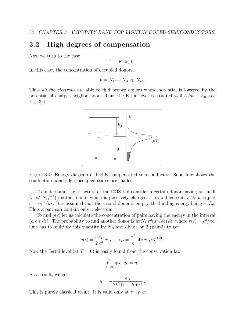
Figure 3.4: Energy diagram of highly compensated semiconductor. Solid line shows theconduction band edge, occupied states are shaded.
To understand the structure of the DOS tail consider a certain donor having at small(r � N
−1/3D ) another donor which is positively charged . Its influence at r � a is just
ε = −e2/κr. It is assumed that the second donor is empty, the binding energy being ∼ E0.Thus a pair can contain only 1 electron.
To find g(ε) let us calculate the concentration of pairs having the energy in the interval(ε, ε+dε). The probability to find another donor is 4πNDr
2(dr/dε) dε, where r(ε) = e2/κε.One has to multiply this quantity by ND and divide by 2 (pairs!) to get
g(ε) =3
2
ε3Dε4ND , εD =
e2
κ(4πND/3)1/3 .
Now the Fermi level (at T = 0) is easily found from the conservation law∫ µ
−∞g(ε) dε = n .
As a result, we get
µ = − εD21/3(1−K)1/3
.
This is purely classical result. It is valid only at rµ � a.
3.3. SPECIFIC FEATURES OF THE TWO-DIMENSIONAL CASE 35
Long-range fluctuations
At 1 −K � 1 it is a large and important effect because screening is weak. To obtain anestimates we can repeat the discussion for K � 1 and replace the donor concentrationby the total concentration, Nt, of donors and acceptors. In this way we get for a typicalpotential energy of an electron,
γ(R) =e2
κR(NtR
3)1/2 .
It also diverges at large R.How the screening takes place. The excess fluctuating density is
∆N = (NtR3)1/2/R3 .
They can be neutralized at ∆N = n leading to the expression for the screening length,
n =(Ntr
3s)
1/2
r3s
→ rs =22/3N
−1/3t
(1−K)2/3.
The random potential amplitude is
γ(rs) =e2N
2/3t
κn1/3.
It increases with decreasing n.Here we disregarded the states with several extra electrons which are important very
deep in the gap.
3.3 Specific features of the two-dimensional case
In high-mobility heterostructures the two-dimensional electron gas is separated from thedoped region by a relatively wide undoped region, spacer, with thickness s. The fluctuationsof the charged donors create a random potential Fb(r) in the 2DEG plane. The reasonto introduce a spaced is that the random potential becomes smooth and transport cross-section a small factor 2pF s/h due to low-angle scattering.
To calculate this potential it is practical to assume that the spatial distribution ofcharged donors in the doped plane is random and not correlated,
〈C(r1)〉 = 0 , 〈C(r1)C(r2)〉 = C δ(r1 − r2) . (3.6)
For the field Fb(r) we obtain
Fb(r) =e2
κ
∫ C(r′) d2r′√|r− r′|2 + s2
= 2πe2
κ
∫ d2q
qC(q) eiq·r−qs . (3.7)

36 CHAPTER 3. IMPURITY BAND FOR LIGHTLY DOPED SEMICONDUCTORS.
Here
C(q) =∫ d2r
(2π)2C(r) e−iq·r → 〈C(q1)C(q2)〉 = C(2π)2δ(q1 + q2) . (3.8)
As a result, we obtain
〈F 2b (r)〉 = 2πC
∫ ∞qmin
dq
qe−2qs . (3.9)
Here qmin ∼ 1/L where L is the linear dimension of the sample. Denoting
W ≡ e2
κ
√2πC (3.10)
we have √〈F 2
b 〉 ≈ W√
ln(L/2s) . (3.11)
For GaAs heterostructure with C = 1.0 × 1011 cm−2 we have W = 9.2 meV. That meansvery large fluctuations of bare potential in a macroscopic sample.
Electron screening removes this divergence. In the linear approximation it can beaccounted for by replacing q by q + qs in the denominator of the integrand of Eq. (3.9)
〈F 2b (r)〉 = 2πC
∫ ∞qmin
dq
q + qse−2qs . (3.12)
where
qs = 2πe2
κ
dn
dµ, (3.13)
where n is the electron density while µ is the chemical potential of electrons. Followingprevious derivation we obtain√
〈F 2b 〉 =
W
2(qss), for qss� 1 . (3.14)
We obtain that the linear screening dramatically reduces the potential since qs = 2/aBwhere aB is the Bohr radius. However, this estimate does not hold if the relative changein concentration is not small relative to the average concentration. Then the fluctuationsin the long-range potential are of the order W .
The main idea of nonlinear screening is that entire plane screens each Fourier harmonicof the impurity charge distribution independently. The excess average square density ofimpurities in a square of area R × R is
√CR2/R2 =
√C/R. If the electron density n is
much greater, n �√C/R, then the harmonic with the scale R will be screened linearly.
However, the harmonics with R �√C/n are not screened effectively, and 2DEG density
becomes strongly inhomogeneous at the scale R. As a result, we arrive at the picture thatharmonics in the impurity distribution with wavelengths R � Rc =
√C/n are screened
linearly, while those with R� Rc are screened very poorly.For large electron density, Rc � s, and all significant harmonics in the bare potential
are screened linearly. If the electron density is lowered, the nonlinear screening length

3.3. SPECIFIC FEATURES OF THE TWO-DIMENSIONAL CASE 37
becomes larger, and eventually, for small enough electron density Rc becomes of the sameorder as s. At small densities, the fluctuations include all harmonics between s and Rc,and quantitative results can be obtained only numerically. We come to a conclusion thatat some electron density a percolation between metallic droplets disappears, and a metal-to-insulator transition takes place. An of the critical electron density is
ncβ =
√C
s, β ≈ 0.1 . (3.15)
An extremely interesting problem appears in an external magnetic field. We will not discussit here.

38 CHAPTER 3. IMPURITY BAND FOR LIGHTLY DOPED SEMICONDUCTORS.
Chapter 4
DC hopping conductance in lightlydoped semiconductors: Generaldescription
4.1 Basic experimental facts
At large temperatures semiconductors possess an intrinsic electrical conductivity due tothermal activation of carriers across the energy gap. In this case the electron, n, and hole,p, concentrations are equal and exponentially temperature dependent,be
n = p =(2πkT
√memh)
3/2
4π3h3 e−Eg/2kT . (4.1)
Due to the activation energy Eg/2 the concentration rapidly decreases with the tempera-ture. At low temperatures it becomes less than the concentration contributed by impuri-ties. In this region the conduction is called extrinsic since it depends on the impurities.A schematic plot of temperature dependence of the conductance is shown in Fig. 4.1 Theregion A corresponds to intrinsic conduction, while the regions B − D correspond to ex-trinsic conductance. If the impurities are shallow, then there exists the region B which iscalled the the saturation range. In this range, all the impurities are ionized and hence thecarrier concentration is temperature independent. Consequently, the temperature depen-dence of resistivity is determined entirely by the carrier mobility. For example, a decreasein resistivity can be explained by a weaker phonon scattering.
Further decrease in the temperature leads to a gradual freeze-out of the electrons whichare recaptured by donors (for n-type material).
Experimentally, the temperature dependence of the resistivity in the region C oftenshows only one activation energy, ε1,
ρ(T ) = ρ eε1/kT , (4.2)
where ε1 is close to the ionization energy E0 of an isolated donor.
39

40 CHAPTER 4. DC HOPPING CONDUCTANCE ...
1/T
ln ρ
A B C D
Figure 4.1: Schematic temperature dependence of the resistivity of a lightly doped semicon-ductor. A - region of intrinsic conductance, B saturation region of impurity concentration,C - freeze-out region, D - hopping conduction region.
At lower temperatures, hopping between the impurities without excursion to the con-duction band becomes most important (region D). The experimental results for p-typeneutron-doped Ge is shown in Fig. 4.2. Each curve corresponds to a different acceptor(Ga) concentration. As a result, an interpolation formula for the regions C and D has theform
ρ−1(T ) = ρ−11 e−ε1/kT + ρ−1
3 e−ε3/kT . (4.3)
The 1st item corresponds to the band conductivity, and it is almost independent of theacceptor concentration. The second one corresponds to hopping conduction (it will clearlater why we gave the subscript 3 for it). We see that that hopping conduction hasa noticeable activation energy ε3, though it is small compared to ε1. It arises due to thedispersion of impurity levels.In hopping over donors, an electron emits and absorbs phononsthat results in an exponential temperature dependence.
When impurity concentration increases, it first somehow enhances that activation en-ergy. However, a further increase in the concentration increases an overlap between thewave functions of neighboring centers. At NA = 1017 cm−3 the activation energy ε3 van-ishes, and the conductance crosses over to a metallic one.
A characteristic feature of hopping which is evident from Fig. 4.2 is an extremely strongdependence of ρ3 on impurity concentration. It can be represented as
ρ3 = ρ03 ef(ND) (4.4)
where ρ03 and f(ND) are power-law functions of the impurity concentration. The expo-nential dependence is rather clear - it is just due to change of the wave-function overlapintegrals.
What is also important is that both ρ3 and ε3 are strong functions of the degree ofcompensation. The dependence ε3(K) is non-monotonous, it decreases sharply at first,then has a minimum at K ≈ 0.4, and then grows rapidly at K → 1.

4.2. THE ABRAHAMS-MILLER RESISTOR NETWORK MODEL 41
Figure 4.2:
In addition to the band and hopping mechanisms of conduction , semiconductors withlow compensation K ≤ 0.2 display another activated mechanism which manifests itselfnear the Mott transition. The mechanism contributes one more term of the form
ρ−12 e−ε2/kT .
We will not discuss this feature in detail.
4.2 The Abrahams-Miller resistor network model
4.2.1 Derivation
To calculate the hopping conductance we shall use the so-called resistor network modelintroduced my Miller and Abrahams. First, starting from electron wave functions we shallcalculate the hopping probability between the centers i and j with the absorption andemission of a phonon. Then we shall calculate the number of i → j transition per unittime. In the absence of an electric field there is a detailed balance, and this number isexact equal to the number of reverse transitions. However, in the presence of the of a weak

42 CHAPTER 4. DC HOPPING CONDUCTANCE ...
electric field an imbalance appears, and a current appears proportional to the voltage dropbetween the centers. Consequently, we can introduce an effective resistance Rij of a giventransition, and thus the whole problem is reduced to calculating of effective resistance ofa network of random resistors. This way will be traced in detail below.
Consider two donors having the coordinates ri and rj and sharing 1 electron. Forsimplicity, let us assume that the distance between the donors is large, so the overlapwill be weak. In the absence of the overlap the wave function Ψi ≡ Ψ(r− ri) satisfies theSchrodinder equation with the potential U = −e2/κ|r−ri|. Within the framework of linearcombinations of atomic orbitals (LCAO) method, the system is represented by symmetricand asymmetric combinations of atomic wave functions,
Ψ1,2 =Ψi ±Ψj√
2√
1±∫dr Ψ∗iΨj
(4.5)
The corresponding energies are obtained from the Hamiltonian
H = H0 −e2
κ|r− ri|− e2
κ|r− rj|(4.6)
are
E2,1 = −E0 −e2
κrij± Iij , (4.7)
where E0 is the energy is an isolated donor, while Iij is the energy overlap integral is
Iij =∫
Ψ∗iΨje2
κ|r− rj|dr−
∫Ψ∗iΨj dr
′∫ e2|Ψi|2
κ|r− rj|dr . (4.8)
Now let us consider a simple case where the donor state is connected to a single extreme inthe Brillouin zone center. Then we can split integral into a sum over crystal cells and usethe fact that the envelope function is almost constant over a cell. The same can be donewith potential energy which contains |r− rj| � a0. The cell integrals |un,0|2 give unity. Inthis way we come to the expression
Iij =∫Fi(r)Fj(r)
e2
κ|r− rj|dr−
∫Fi(r
′)Fj(r′) dr′
∫ e2|Fi|2
κ|r− rj|dr . (4.9)
For a hydrogen-like function
F (r) =1√πa3
e−r/a
we get
Iij =2
3
(e2
κa
)(rija
)exp
(−rija
). (4.10)
Note that there is a more accurate calculation which does not assume the overlap integralto be small. It differs from Eq. (4.10) by replacing 2/3→ 2/e. The general feature of theenergy overlap integral is that it can be expressed as
Iij = I0 exp(−rija
)(4.11)

4.2. THE ABRAHAMS-MILLER RESISTOR NETWORK MODEL 43
where I0 is of the order of the effective Bohr energy and only weakly dependent on rij.In important fact is that the electron interacts also with the other charged impurities
surrounding the center by some potential W (r). As a result, for the majority of donors,
∆ji>∼ Iij , where ∆j
i ≡ W (rj)−W (ri) . (4.12)
Consequently, the potential W should be included into the Hamiltonian. The simplestsituation case is when ∆j
i � Iij. Then for the two lowest states we can show that
Ψ′i = Ψi +Iij
∆ji
Ψj ,
Ψ′j = Ψj −Iij
∆ji
Ψi . (4.13)
Despite of the the fact that an admixture of the “foreign” state is small, it leads to thecharge transfer on distance rij.
Now let us consider phonon-induced transitions and assume that only a single branchof acoustic phonons is present. The transition probability i → j with absorption of onephonon is
γij =2π
h
V0
(2π)3
∫|Mq|2 δ(hsq −∆j
i ) dq , (4.14)
where V0 is the volume of the crystal, s is the speed of sound, q is the phonon wave vector,while
Mq = iD
√hqNq
2V0ρ
∫Ψ′je
iq·rΨ′i dr (4.15)
is the matrix element of electron-phonon interaction. Here D is the deformation potentialconstant, Nq is the Planck function, ρ is the crystal density. Substituting the functions Ψ′
and coming to the envelope functions we rewrite the previous expression in the form
Mq = iD
√hqNq
2V0ρ
{Iij
∆ji
[∫F 2j e
iq·r dr−∫F 2i e
iq·r dr]
+
1−(Iij
∆ji
)2 ∫ FiFje
iq·r dr
, (4.16)
To estimate the integral let us evaluate two dimensionless parameters,
qrij = ∆jirij/hs and qa = ∆j
ia/hs .
Since ∆Ji ≈ e2N
1/3D κ−1 and Rij ≈ N
−1/3D we see that qrij is usually large (20-30) while qa is
of the order 1. The characteristic length of variation of FiFj across the line connecting twocenters is or the order
√rija. Thus the last integral in Eq. (4.16) is strongly suppressed
due to oscillatory factor, and it can be neglected. The first two integrals can be combinedin the form (
eiq·rij − 1) ∫
F 2i e
iq·r dr =(eiq·rij − 1)
(1 + q2a2/4)2.

44 CHAPTER 4. DC HOPPING CONDUCTANCE ...
The last equality is valid for hydrogen-like wave functions. Finally we obtain
|Mq|2 =hqD2
2ρV0s
(Iij
∆ji
)2Nq(1− cos q · rij)
(1 + q2a2/4)4. (4.17)
Substituting this expression into (4.14) and using the fact that qrij � 1 we get the finalexpression
γij = γ0ij e−2rij/aN(∆j
i ) (4.18)
where
γ0ij =
D2∆ji
πρs5h4
(2e2
3κa
)2 (rija
)2 1
[1 + (∆jia/2hs)
2]4,
N(∆ji ) =
[exp(∆j
i/kT )− 1]−1
. (4.19)
Let n = (0, 1) are the occupancies of ith donor which fluctuate in time. The transitioni→ j is possible if ni = 1, nj = 0. Therefore the average number of electrons which maketransitions is
Γij = 〈γijni(1− nj)〉 . (4.20)
The average should be taken with respect to time. Here we make a fundamental assumptionthat the occupancies can be replaced by their average numbers, 〈ni〉 ≡ fi, while the energiescan be replaced by self-consistent energies
εi =acc∑l
e2
κ|ri − rl|−
don∑k 6=i
e2(1− fk)κ|ri − rk|
. (4.21)
In this approximation we can put ∆ji = εj − εj ≡ εij to obtain,
Γij = γ0ij e−2rij/aN(εj − εi) fi(1− fj) . (4.22)
For the reverse process we get
Γji = γ0ij e−2rij/a [N(εj − εi) + 1] fj(1− fi) . (4.23)
The current between the centers j and i can be written as
Jij = −e(Γij − Γji) . (4.24)
In the absence of an electric field
fi = f 0i =
[1
2exp
(ε0 − µkT
)+ 1
]−1
(4.25)
where ε0 is the average energy at the site at E = 0, while factor 1/2 enters because thereare 2 possible spin states at the site i. In fact the energies ε0 and the functions f 0
i aremade self-consistent by Eq. (4.21).

4.2. THE ABRAHAMS-MILLER RESISTOR NETWORK MODEL 45
It can be easily seen that a detailed balance is present, and there is no current. Theelectric filed, first, redistributes the electrons between the donors, f 0
i → f 0i + δfi. We
describe these changes by small additions δµi,
fi(E) =
[1
2exp
(ε0 − δµi − µ
kT
)+ 1
]−1
(4.26)
Secondly, the field affects the donor level energies,
εi = ε0i + δεi , δεi = eE · ri +
e2
κ
don∑k 6=i
δfk|ri − rk|
. (4.27)
Would the circuit be broken, a new equilibrium with δµi + δεi = 0 will result. Howveer inthe case of conductance, δµi + δεi 6= 0. Assuming all the correction to be small (linear inE effects) we can expand all the energies up to the first order in δεi and δµi. After suchmanupulation we obtain
Jij =eΓ0
ij
kT[δµi + δεi − (δµj + δεj)] (4.28)
The latter equation can be expressed as the Ohm’s law
Jij = R−1ij (Ui − Uj) (4.29)
where
Rij = kT/e2Γ0ij , Γ0
ij = γ0ij e−2rij/aN(εj − εi) f 0
i (1− f 0j ) , (4.30)
−eUi = δµi + δεi = eE · ri +e2
κ
don∑k 6=i
δfk|ri − rk|
. (4.31)
The quantity −eUi can be regarded as a local value of the electrochemical potential onthe donor i counted from the chemical potential µ. Thus Ui − Uj is the voltage drop onthe transition i → j while Rij is its resistance. We end at the problem of calculating ofeffective resistance of a random resistor network keeping the potentials at the electrodesconstant.
4.2.2 Conventional treatment
Let us analyze the expressions for the resistances Rij and assume the temperatures to below,
kT � |ε0i − ε0
j |, |ε0i − µ|, |ε0
j − µ| .
Then we can extract the functions strongly dependent on the distance rij and on theenergies,
Γ0ij ≈ γ0
ij e−2rij/a e−εij/kT (4.32)

46 CHAPTER 4. DC HOPPING CONDUCTANCE ...
where
εij =1
2(|εi − εj|+ |εi − µ|+ |εj − µ|) . (4.33)
Now it is convenient to introduce the quantity
ξij =2rija
+εijkT
(4.34)
to express random resistors as
Rij = R0ij exp(ξij) , R0
ij = kT/e2γ0ij . (4.35)
The main feature of the problem is an exponentially wide range of resistances. It is clearthat doth averaging of conductances and resistances will lead to wrong answers. A correctmethod of averaging is suggested by the mathematical theory of percolation.
Chapter 5
Percolation theory
The term “percolation” has been introduced in 1957 by Broadbent and Hammersley in con-nection with a new class of mathematical problems. We shall start with general descriptionand then will map them to the hopping conductance.
5.1 Lattice problems
5.1.1 “Liquid flow” definition
Imagine an infinite lattice with bonds between the adjacent sites which permit the flow inboth directions, and that each wet site will instantly wet the adjacent sites. The variousproblems follow from introduction random elements into the theory.
Bond problem
Assume that each bond in the lattice can be other blocked, or unblocked. Let the proba-bility of any bond to be unblocked is “x”. The distribution of unblocked and blocked bondsremains constant in time.
If a random site is wet, then there are 2 possibilities. The initial site will wet eithera finite or an infinite number of other sites. The key quantity is the probability of arandom initial site to wet an infinite number of other sites. In the infinite lattice thisprobability depends only on x. Let us denote it as P b(x). The bond problem is illustratedin Fig. 5.1 (left panel), while the function P b(x) is plotted for different lattices in the rightpanel. Curves 1,2 and 4 correspond to 3D lattices, the rest to 2D ones. When x is smallP b(x) ≡ 0 since the blocked bonds prevent the liquid to spread far from the initial site.On the other hand, as x approaches 1, so does P b(x). A very important quantity is thepercolation threshold, xx, defined as an upper limit for the x-values for which P b(x) = 0.When x− xc � 1, one has
P b(x) ∼ (x− xc)β (5.1)
47

48 CHAPTER 5. PERCOLATION THEORY
E + Uo o
Eo
1/boA
E
Figure 5.1:
where b is a critical exponent. The situation resembles type II phase transitions. Note thatall the conclusions are valid for an infinite lattice.
One can also define the probability to wet N other sites, P bN(x). P b
N(x) differs from 0at 0 < x < 1, but at N � 1 it is small for x < xc. We can define
P b(x) = limN→∞
P bN(x) .
An example of the bond problem - an orchard which is planned in the form of a squarelattice. It is known that a diseased tree contaminates another tree away at the distancer with the probability f(r). It is required to find a minimum lattice period hmin to avoidepidemy. The solution is obvious,
f(hmin) = xc . (5.2)
Site problem
For the site problem, sites can be either blocked, or unlocked, while the bond are assumedto be ideal. Blocked sites permit no flow in any direction, they cannot be wet. Let x bethe fraction of unblocked sites while P s(x) be a probability for a random site to wet infinitenumber of other sites.
The probability function P s(x) is plotted in the left panel of Fig. 5.2, while a realizationof the site problem in shown in the right panel. One can see that there is a percolationthreshold which depends in the lattice type.
5.1.2 Cluster statistics
Both the site and both problems are usually discussed in terms of cluster statistics, ratherin terms of liquid flow. Let us apply this approach to the site problem. Imagine that a

5.1. LATTICE PROBLEMS 49
Figure 5.2:
fraction x of the sites is painted black, while the rest sites are painted white. Any twoadjacent sites are connected if both are black. A chain of such connected clusters becomesa cluster. For example in the right panel of Fig. 5.2 there are 3 clusters - one consists of 5black sites while two consist of 3 black sites.
When x is small, then there are only small clusters. As we approach the percolationthreshold, several clusters may come together, and the mean cluster size increases. Atx→ xc an infinite black cluster is born. It resembles a random network which permeatesthe entire lattice, while smaller since finite clusters exist in the “pores”, see Fig. 5.3.Actually, P s(x) has a meaning of the density of the infinite cluster. Similarly, a proper
Figure 5.3:

50 CHAPTER 5. PERCOLATION THEORY
definition for the bond problem can be formulated.It is assume that no more than one infinite cluster can exist in a lattice. Than brings
us to an important application of the site problem - a crystalline solution of ferromagneticatoms (with a fraction “x”) in a non-magnetic host. Assuming nearest-neighbor ferromag-netic interaction we arrive at the ferromagnetic phase transition at zero temperature as apercolation threshold for the site problem. Consequently,
• the transition takes place at x = xc;
• the saturation magnetization at T = 0 for x > xc can be expressed through thedensity of the infinite cluster,
M |T=0 = µ0Ps(x) (5.3)
where µ0 is the atomic magnetic moment.
Another important application is the aforementioned Anderson transition. The appearanceof the extended states is similar to formation of an infinite black cluster.
Now let us introduce relevant quantities for the cluster statistics. Let ns be the numberof clusters containing s sites, per site of an infinite lattice. Then the fraction of sitesbelonging to an infinite cluster is
P (x) = x−∑s
sns . (5.4)
The second important quantity is the mean cluster size,
S(x) =
∑s s
2ns∑s sns
. (5.5)
According to numerical estimates, S(x) becomes infinite at xc,
S(x) ∼ |x− xc|−γ , (|x− xc| � 1) , (5.6)
where γ is a critical exponent. Note that Eq. 5.5 calculates a weighted average which isdivergent. A simple average would be regular because
limx→xc
∑s
sns = xc .
The majority of sites remain in clusters with s ∼ 1 even at x = xc.According to numerical estimates, ns near the percolation threshold behaves as follows.
There is a critical number sc of the sites in the cluster, which grows at x→ xc + 0 and atx→ xc − 0,
sc(x) ∼ |x− xc|−∆ , ∆ > 0 . (5.7)
If s� sc and s increases the quantity ns decreases according to some power law, while ats� sc it decreases exponentially. Consequently, the numerator of Eq. (5.5) is determined

5.1. LATTICE PROBLEMS 51
by the clusters with s ≈ sc, which we will refer to as critical clusters. The divergence ofS(x) means that the number of sites in critical cluster increases.
The third important quantity in the percolation theory is the correlation function. Letus define a function g(ri, rj) as equal to 1 if both sites are black and belong to the samecluster, and 0 otherwise. Now we can introduce the pair correlation function as
G(r, x) = G(ri − rj, x) = 〈g(ri, rj)〉 . (5.8)
Naturally, G(r, x) does to zero at r → ∞ because ns decreases with s. At the distancessmaller that the average size of the critical cluster which we will denote as L(x), thecorrelation is governed by the clusters with s� sc(x). Consequently, G(r, x) decreases asa power law of r. If r � L(x), the exponentially rare clusters with s� sc(x) are dominant,and G(r, x) decreases exponentially. The length to the critical clusters, L(x), is called thecorrelation length. Since the number of sites in the critical clusters grow at x → xc ± 0,the correlation length must grow if one approaches the percolation threshold,
L(x) ∼ |x− xc|−ν , (|x− xc| � 1) . (5.9)
Here ν is the critical exponent of the correlation length. It is usually thought that thecritical exponents γ, ∆ and ν are the same whether x > xc or x < xc, and that there existsa sort of cluster-pore duality (see Fig 5.3). Thus, at x < xc the quantity L(x) is a typicalradius of clusters, while at x > xc it is a typical radius of the pores. Near xc the correlationlength introduces a typical distance (“period”) between the nodes of the network.
5.1.3 Percolation through a finite lattice
Consider a finite lattice containing ` sites per side. Let all the sites be initially white. Wewill randomly paint some sites black, slowly increasing the fraction x. At some x = xc` theblack cluster will connect opposite sides. We will consider xc` as a percolation thresholdfor a finite lattice. If we permit the procedure, the arrangement of the black sites, as wellas xc` will be different. Therefore, xc` is the random quantity, and we can define the truepercolation threshold as
xc = lim`→∞〈xc`〉 . (5.10)
Another variation of the same theme is to define x as the probability for a site to be blackrather that as the fraction of the black sites. In a finite systems, these two definitions leadto different valuers of xc` and 〈xc`〉 due to fluctuations. We can say that the 1st definitioncorresponds to a micro-canonical ensemble while the 2nd one - to the canonical ensemble.
Figure 5.4 shows the distribution function f` of xc` in a canonical ensemble for the siteproblem on a square lattice. This figure was obtained by Monte Carlo simulations. Thedistributions are nearly Gaussian in shape. The larger the side the lower the dispersionW 2` = 〈(xc` − 〈xc`〉)2〉. It was shown that W` obeys the power law
W` = B`−1/ν , (5.11)

52 CHAPTER 5. PERCOLATION THEORY
Figure 5.4:
while the average threshold obeys the law
〈xc`〉 = xc + A`−1/λ . (5.12)
In three dimensions, ν ≈ 0.9 and λ ≈ 1. It can be shown that the exponent ν is the sameas for the correlation length.
As an example of percolation between the opposite faces for the 3D bond problem letus consider electrical conductivity of a large cube in which the unblocked bonds are repre-sented by standard resistors. The blocked bonds are assumed to have infinite resistance,Fig. 5.5. If the cube is large, then the conductivity differs from zero only at x > xc(b),while at 0 < x− xc � 1 one has
σ(x) ∼ (x− xc)t , (5.13)
where t is yet another critical exponent. It is clear that to find σ it is not enough to knowP b(x) since also a topological structure of the infinite cluster is important.
5.1.4 Summary
We have presented 3 definitions of the percolation problem: liquid flow, cluster statistics,and percolation through a finite lattice. It can be shown that critical phenomena are thesame in all three formulations. The typical questions to be answered:

5.2. CONTINUOUS PROBLEMS 53
Figure 5.5: A random resistor network between two electrodes.
1. What is the percolation threshold xc?
2. What are the critical exponents β, γ , ν and t?
3. How do dimensionality and lattice geometry affect the above mentioned quantities?
4. What is the topology of finite and infinite clusters?
The values of the percolation thresholds are summarized in Table 5.1 In the Table 5.2 themost important critical exponents are presented. The majority of values in the tables werefound by numerical simulations, however some results are obtained analytically. In rarecases, experimental methods were used.
The modern point of view is that the critical exponents depend only on the dimension-ality of the problem, and in this way they are universal.
5.2 Continuous problems
Suppose a random continuous function V (r) is defined in the entire space by its correlations,such that 〈V (r)〉 = 0. Then let us paint black the regions where V (r) < V and leave otherregions white. As V changes from −∞ to∞ the volume of black region changes form zeroto all space, see Fig. 5.6. As V increases, the black regions grow, and at some Vc theymerge into an “ocean” The quantity Vc is called the percolation threshold. Such a “liquid-flow” definition can be easily reformulated into the “cluster statistics”, or “finite-volumepercolation” ones.
One can easily map the continuous problem to the lattice one. Assume a lattice withso fine grid that the potential does not change. Then fix V and consider all the sites inthe black regions to be black while the other sites - to be white. The the fraction of theblack sites is
x = θ(V ) ≡∫ V
−∞F (V ′) dV ′ (5.14)

54 CHAPTER 5. PERCOLATION THEORY
Table 5.1: From the book [1]
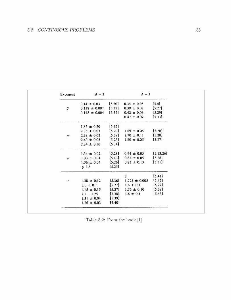
5.2. CONTINUOUS PROBLEMS 55
Table 5.2: From the book [1]

56 CHAPTER 5. PERCOLATION THEORY
where θ(V ) is the space fraction of the black sites, while F (V ) is the distribution functionof the quantity V . The percolation threshold then can be defined by equating the quantity
θc =∫ Vc
−∞F (V ) dV (5.15)
to the percolation threshold xc of the site problem. Physically it means that the distri-butions of black and white sites are now correlated according to the function V (r). Thisproposition is very important for practical calculation of θc.
Along with the above mentioned “percolation through black”, one can define a “perco-lation through white” with some threshold V ′c . In the two-dimensional case Vc = V ′c = 0,and θc =0.5. The situation in 3 dimensions is more complicated. Only an inequalityVc ≤ V ′c does exist, so the following 3 situations are possible:
1. V < Vc and there is percolation through white, but not through black;
2. Vc ≤ V < V ′c and there is percolation through both black and white;
3. V ≥ V ′c and there is percolation through black, but not through white.
It the potential is statistically symmetric, then
Vc ≤ 0 , V ′c ≥ 0 , and θc ≤ 0.5 . (5.16)
The quantity θc has been extensively studied for various distribution functions of therandom potential. A typical value of θc for Gaussian potentials is θc=0.17.
5.3 Random site problems
The most important problems for hopping conductance are the so-called random-site prob-lems. Random sites are the sites chaotic distributed in space, the average number N ofsites per unit volume being known. If one introduced some function ξij(rij), the two sitesare considered bonded if, for some number ξ,
ξij ≤ ξ . (5.17)
Eq. (5.17) is referred to as the bonding criterion. If two sites are bonded either directly,or via some other sites, then they form a cluster. It is required to find the percolationthreshold ξc, i. e. the lowest bound of the parameter ξ which still permits an infinitecluster.
The simplest example of the bonding criterion is
rij ≤ r , (5.18)
which is met if the state j is located within the sphere of the radius r centered at the sitei. Consequently, the problem has a very simple geometric interpretation: spheres of radius

5.3. RANDOM SITE PROBLEMS 57
r are constructed around all the sites, and we must find the lowest value r = rc whichallows endless chain of sites in which each cite lies inside the sphere about the precedingsite, see Fig. 5.7 We will term the quantity rc the percolation radius. Occasionally it ismore convenient to construct spheres with radius r/2 and calculate the value that allowsfor an infinite cluster of overlapping spheres.
The percolation threshold rc depends solely on the concentration N and is must beproportional to N−1/3. In most cases people consider the threshold value
Bc = (4/3)πNr3c (5.19)
of the dimensionless parameter B = (4/3)πNr3 which corresponds to an average numberof bonds per site. This problem is often called the sphere problem, or the disk problem in2D case (where Bc = πNr2
c ).
A physical implementation of this problem is a ferromagnetism of a dilute crystallinemixture of magnetic and non-magnetic atoms, where the exchange forced between magneticatoms are modeled by a finite-radius interaction with the interaction radius rint. If rint ismuch greater than the lattice constant so that many sites fall into the sphere of interaction,then we arrive at the sphere problem. However, the problem is a reversed one: knowingrint we have to find N . If the number of sites that fall into the interaction sphere is Z thatfor the lattices of any dimensionality we obviously have
limZ→∞
Zxc = Bc . (5.20)
The critical indices for the random site problems can be introduced in the same way asfor the lattice model. Introducing ns as the number of clusters of size s in a given volumewe can rewrite scaling properties in a similar way in terms of ξ − ξc.
In some important cases the bonding criterion is fulfilled on a complex surface ratherthan on a sphere. Then it should be written in the form
ξij ≡ φ(rij) ≤ ξ . (5.21)
Here ξ > 0, and φ(r) is a monotonously increasing homogeneous function of xij, yij, andzij. The equation φ(rij) = ξ define a surface which replace the sphere in the constructionsdiscussed above. In particular, we can define Bc as NVξc . It can be shown that the valuesBc are the same for all the surfaces which can be obtained from each other via a linearcoordinate transformation,
x′k =∑`
Ak`x`
since such transformation does not change the topology of the system. Thus the thresholdvalues Bc for ellipsoids and spheres are the same.

58 CHAPTER 5. PERCOLATION THEORY
5.4 Electric conductivity of random networks of con-
ducting bonds. Infinite cluster topology
As we have mentioned for the case of lattice models, the electric conductivity of a latticeof conducting and non-conducting bonds behaves as
σ(x) ∼ (x− xc)t (x ≥ xc). (5.22)
The aim of this section is to discuss the critical exponent t. There are few ways to studythis problem: an experimental (by punching holes in a graphite paper, cutting bonds ina metallic grid, etc), computer simulations, etc. It appears that the results both for siteand bond problems are closed in value. It seems logical that these values will retain alsofor the continuum version. What we want to do now is to relate the conductivity to otherproperties of the infinite cluster, namely, with its density P (x) and the “period” L(x). Itis clear that these quantities do not contain the full necessary information about σ(x), andwe need some assumptions to relate the critical exponents.
Dead ends
Consider a large cube containing ` units per side. If the infinite cluster resembles a cubiclattice then 1/3 of the bonds form chains that connect the opposite edges of the cube, thenumber of bonds in these chains being ≈ (1/3)P (x)`3. Each chain has ` sites, thereforethe number of parallel chains is ≈ (1/3)P (x)`2. Since the resistance of each bond is ∝ `,the resistance R of the whole cube is ∝ `[P (x)`2]−1. Consequently,
σ(x) ∼ (R`)−1 ∼ P (x) ∼ (x− xc)β . (5.23)
We arrive at the conclusion that t = β. However, we know that t > β, see Table 5.2. Thatleads to a conclusion that almost all the “mass” of the infinite cluster is concentrated in itsdead ends, sii Fig. 5.8. These chains contribute to P (x), but not to σ(x). The insufficiencyof the infinite cluster can be also due to redundunt
The nodes and links model
This is the most used model (Skal-Shklovskii-De Gennes, SSDG) assumes that there is abackbone network with w mean size L ∼ (x−xc)−ν , and that this back bone cartries deadends. The part of the backbone is called the link. It is assumed that at least half of thelinks are not doubled. Each link can be twisted, so its length L is larger than L. It thisway we can write at x− xc � 1
L ∼ (x− xc)−ζ , where ζ ≥ ν . (5.24)
A schematic representation of the SSDG model is shown in Fig. 5.9. To proceed let us firstshow that ζ = 1. Let x > xc and cut each bond with the probability (x − xc)/x. As a

5.4. RANDOM NETWORKS.INFINITE CLUSTER TOPOLOGY 59
result, the fraction of unbroken bonds will become x[1 − (x − xc)/x] = xc. Consequently,we arrive at the percolation threshold for the original lattice. Now notice that to cut a linkwe must cut one of its constituent bonds (we have assume that the links are not doubled!).Thus, the probability for a link to be broken is proportional to L and equal L(x− xc)/x.We can assume the percolation threshold for a backbone to be equal to some yc. EquatingL(x− xc)/x = yc we find that ζ = −1. We note that in 2D case ν > 1, and it means thatSSDG model does not hold, and that duplication of links is crucially important. However,for d = 3 ν3 ≈ 0.9, and L ∼ L1.1. Note that the twistness appears very weak comparing tothe cases of the random walk, L ∼ L2 and of the self-avoiding random walk, L ∼ L5/3.
Now let us calculate σ(x) If resistance of each bond is R0 then the resistance of a cubewith side L is R0(L/`0) where `0 is the bond length. At the scales larger than L the infinitecluster is homogeneous. Therefore σ(x) can be calculated as an effective conductivity of acube with the side of the order of the correlation length. We get
σ(x) = R−1L2−d = R−10 (L/`0)−1L2−d = R−1
0 `2−d0 (x− xc)1+ν(d−2) . (5.25)
As a result,t = 1 + ν(d− 2) . (5.26)
For d = 3 we get t3 = 1 + ν3. Substituting ν3 = 0.9 we obtain t3 = 1.9 while the numericalvalue is 1.7. We conclude that SSDG model is not very accurate. However it is extensivelyused because it is simple and qualitatively correct. It has been extensively used in thetheory of dilute ferromagnets, granular superconductors, conductivity and Hall effect indisordered systems. The model has been also extended to take in some way into accountthe bond doubling. It makes the model more accurate.
The most important extension (Pike and Stanley) is to discriminate between red andblue backbone bonds. Breaking a red bond breaks the link itself. It was further suggestedthat blue bonds from blobs connected by singly connected chains. The number of red bondbetween the nodes has also be scaled as L′ ∼ (x− xc)−1. A finite size of the blobs removesthe limitation of the model for the cases when ν > 1, in particular in 2D case. It seemsthat the combined nodes-links-blobs model describes properly the structure of the infinitecluster.
Scaling hypothesis and calculation of σ(x)
Another way to estimate the exponent t is to suggest that the large-scale structure ofthe network remains self-similar as the system approaches the percolation threshold. Thesecond assumption to be maid is that the resistance is determined only by a large-scalestructure. The two assumptions allow one to relate t and ν in a simple way.
Let us denote τ = x−xc and examine the systems at two values of τ , such that τ2 < τ1.Since L ∼ |τ |−ν , the dimensions of the system will increase by the factor L(τ2)/L(τ1) =(τ1/τ2)ν . We assume that we also scale the distance between the contacts and the potentialdifference by the same factor. We conclude that the current distribution in the bond willnot be affected. Now consider an area element that is perpendicular to the average direction

60 CHAPTER 5. PERCOLATION THEORY
of the current. The number of channel piercing the area will decrease as L(τ1)/L(τ2) =(τ2/τ1)2ν . Thus the current and the conductivity will decrease by the factor (τ1/τ2)2ν . Asa result, in three dimensions t = 2ν, while in two dimensions t = ν. In this way we obtainthe values t3 = 1.80 and t2 = 1.33 close to the experimental ones. The scaling approachhas appeared extremely fruitful during last years and revealed fractal properties of theinfinite cluster.
5.5 Percolation theory and electric conductivity of
strongly inhomogeneous media
We have previously shown that calculation of hopping conductivity can be reduced toconductivity of a random network with an exponentially wide range of resistances. Thesimilar approach is valid also for a continuum.
Suppose that we have a medium in which local conductivity fluctuates as
σ(r) = σ e−ξ(r) , and (5.27)
〈[ξ(r)− 〈ξ〉]2〉 � 1 . (5.28)
For example, the source of fluctuation can be a band bending due to a random largepotential, and ξ(r) = ε(r)/kT . Here ε(r) is the distance between the Fermi level and thebottom of the conduction band. A similar problem can be also formulated on a resistorlattice with R = R0 e
ξ′ where the random quantity ξ′ is randomly distributed between −ξ0
and ξ0 � 1.To illustrate the method of conductivity calculation let us consider a cubic lattice. Let
us first derive the exponential factor in the effective conductivity. Then we will discussalso a pre-exponential factor, and finally compare the result with the SSDG model.
Consider a simple cubic lattice and select a value ξ in the interval (−ξ0, ξ0). Then letus replace all resistances with ξ′ > ξ by infinite resistances thus breaking the circuits. Letus call the so-obtained conductivity as σ(ξ). The chosen ξ determines the probability of arandom resistance not being broken:
x(ξ) =∫ ξ
−ξ0F (ξ′) dξ′ , (5.29)
where the distribution function F is defined as
F (ξ) =
{1/2ξ0, |ξ| ≤ ξ0
0, |ξ| > ξ0. (5.30)
From Eqs. (5.29),(5.30) we find
x(ξ) =ξ0 + ξ
2ξ0
. (5.31)
Now let us increase the value of ξ from −ξ0 till some value ξc corresponding to the per-colation threshold for the bond problem, xc(b), given by Eq. (5.31). If we that increase ξ

5.5. CONDUCTIVITY OF STRONGLY INHOMOGENEOUS MEDIA 61
from ξc to ξc + 1, the presence of infinite cluster will cause a rapid increase in conductivity.This happens because the correlation length rapidly diminishes as
L(ξ) ∼ `0[x(ξ)− xc(ξ)]−ν ∼ `0ξν0 (ξ − ξc)−ν . (5.32)
Therefore, the number of parallel conducting chains in the infinite cluster network will alsorapidly increase. On the other hand, the change in the individual resistance remains smallif ξ is changed less than 1. Than implies a rapid power-law increase in σ,
σ(ξ) ∼ (ξ − ξc)b , where b > 0 . (5.33)
Let the infinite cluster that is formed when ξ and ξc differ by about one be called the criticalsubnetwork. Its resistance is determined by the highest resistances because, by definitionthese resistances cannot be shunted by lower ones since that would allow for percolationat ξ < ξc. Consequently, for s critical subnetwork we have
σ(ξc + 1) ∼ σ0e−ξc . (5.34)
Further increase of ξ will not raise σ significantly, even though the density of infinite clusterwill rise. Indeed, if we continue to increase ξ we introduce exponentially large resistances.Thus, new chains will be shunted by the critical subnetwork. The expression
σ = σ−ξc0 (5.35)
is the foundation for the hopping conduction theory. According to the Table 5.2, xc(b) =0.25 for the simple cubic lattice. From (5.31) we find ξc = −ξ0/2, and
σ = σξ0/20 (5.36)
This formula is valid only if ξ0 � 1, when the concept of the critical subnetwork is valid.Numerical tests show that the model is practical at ξ0 ≥ 9.
Let us now discuss the pre-exponential factor σ0. From dimensional arguments,
σ0 = c(ξ0)(R0`0)−1 (5.37)
where c(ξ0) is a dimensionless factor which can contain only powers of ξ0. It can be shownthat this power equals to −ν where ν is the correlation length exponent.
To obtain the power, let us suggest another derivation of the conductivity. Considera cube with side ` cut from the infinite lattice. Let us break all the resistances and thenconnect them back in the ascending order until we reach the percolation between theopposite sides. Let the last (greatest) resistance be ξc`. Therefore,
R = R0 eξc` → → σ = (R0`)
−1e−ξc` .
The quantity ξc` is actually random, however for a large system its fluctuations are small.As we have seen, the fluctuations behave as
δξc`ξ0
∼(`0
`
)1/ν
.

62 CHAPTER 5. PERCOLATION THEORY
Now let us increase the cube size `. At some size the conductivity becomes `-independent.We can tell that it happens if the mean square fluctuation approaches unity, or at
` ≈ `0 ξν0 ≡ L0 .
L0 is just the infinite cluster correlation length. For such a cube the difference between ξc`and ξc is negligible. Thus,
σ(ξ0) ∼ (R0`0)−1 ξ−ν0 e−ξc .
A same expression can be easily derived from the node-link model of the infinite cluster.

5.5. CONDUCTIVITY OF STRONGLY INHOMOGENEOUS MEDIA 63
Figure 5.6:
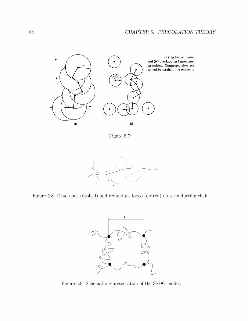
64 CHAPTER 5. PERCOLATION THEORY
Figure 5.7:
Figure 5.8: Dead ends (dashed) and redundunt loops (dotted) on a conducting chain.
L
Figure 5.9: Schematic representation of the SSDG model.

Chapter 6
Hopping conductance
6.1 Dependence on impurity concentrations
In this section, we shall apply the percolation theory to study the dependence of the ρ3
contribution on the impurity concentration.
6.2 The contribution ρ3 as a function of impurity con-
centrations
Let us concentrate on the simplest case of isotropic impurity wave function. In fact, wehave to calculate the resistance of the Abrahams-Miller network of random resistors,
Rij = R0ij e
ξij , (6.1)
where
ξij = 2rij/a+ εij/kT , (6.2)
R0ij = kT/e2γ0
ij , (6.3)
εij = (1/2) (|εi − εj|+ |εi − µ|+ |εj − µ|) . (6.4)
To calculate the resistance let us apply the percolation approach. First suppose that onlythe resistances with ξij < ξ are switched on. Let us gradually increase ξ until we reachthe condition of percolation over conducing resistances. That obviously occurs at ξ = ξc.Increasing ξ from ξc to ξc + 1 results in formation of the critical subnetwork of resistances.This subnetwork shunts all the resistors for which ξ ≥ ξc+1. Consequently, the exponentialpart of the hopping conductivity to the parameters of the problem is given by
ρ = ρ0 eξc . (6.5)
This is the starting point of the theory of hopping conductivity.
65
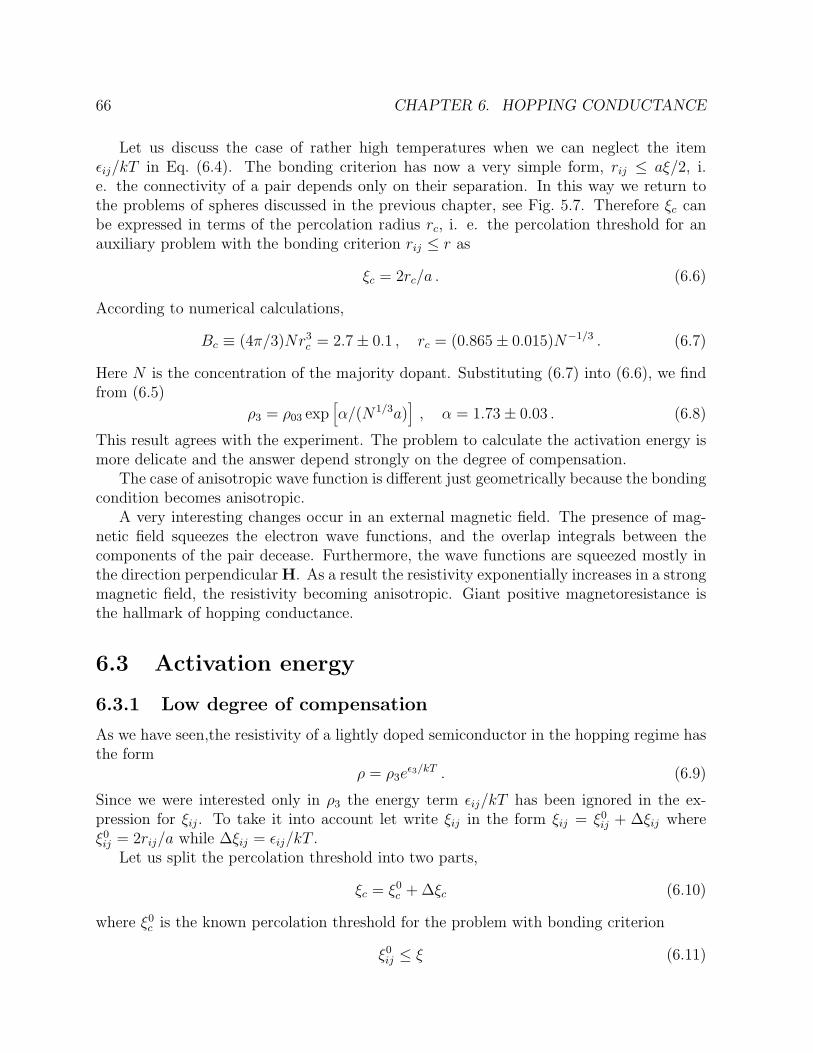
66 CHAPTER 6. HOPPING CONDUCTANCE
Let us discuss the case of rather high temperatures when we can neglect the itemεij/kT in Eq. (6.4). The bonding criterion has now a very simple form, rij ≤ aξ/2, i.e. the connectivity of a pair depends only on their separation. In this way we return tothe problems of spheres discussed in the previous chapter, see Fig. 5.7. Therefore ξc canbe expressed in terms of the percolation radius rc, i. e. the percolation threshold for anauxiliary problem with the bonding criterion rij ≤ r as
ξc = 2rc/a . (6.6)
According to numerical calculations,
Bc ≡ (4π/3)Nr3c = 2.7± 0.1 , rc = (0.865± 0.015)N−1/3 . (6.7)
Here N is the concentration of the majority dopant. Substituting (6.7) into (6.6), we findfrom (6.5)
ρ3 = ρ03 exp[α/(N1/3a)
], α = 1.73± 0.03 . (6.8)
This result agrees with the experiment. The problem to calculate the activation energy ismore delicate and the answer depend strongly on the degree of compensation.
The case of anisotropic wave function is different just geometrically because the bondingcondition becomes anisotropic.
A very interesting changes occur in an external magnetic field. The presence of mag-netic field squeezes the electron wave functions, and the overlap integrals between thecomponents of the pair decease. Furthermore, the wave functions are squeezed mostly inthe direction perpendicular H. As a result the resistivity exponentially increases in a strongmagnetic field, the resistivity becoming anisotropic. Giant positive magnetoresistance isthe hallmark of hopping conductance.
6.3 Activation energy
6.3.1 Low degree of compensation
As we have seen,the resistivity of a lightly doped semiconductor in the hopping regime hasthe form
ρ = ρ3eε3/kT . (6.9)
Since we were interested only in ρ3 the energy term εij/kT has been ignored in the ex-pression for ξij. To take it into account let write ξij in the form ξij = ξ0
ij + ∆ξij whereξ0ij = 2rij/a while ∆ξij = εij/kT .
Let us split the percolation threshold into two parts,
ξc = ξ0c + ∆ξc (6.10)
where ξ0c is the known percolation threshold for the problem with bonding criterion
ξ0ij ≤ ξ (6.11)
6.3. ACTIVATION ENERGY 67
while ∆ξc is the correction which we are going to find.In the case K � 1 let us first ignore the long-range potential. Then the most donor
levels are close to the unperturbed value (which according to our notations corresponds toε = 0) and well separated from the value of chemical potential. Then for overwhelmingmajority of donor pairs we can neglect εi and εj in comparison with µ. As a result,
∆ξij = µ/kT , (6.12)
and
ξc = ξ0c + µ/kT . (6.13)
As a result,
ρ = ρ03 eξ0c+µ/kT , ε3 = 0.99e2N1/3/κ . (6.14)
Since the long-range potential is small comparing to µ it produces only a small correctionto the activation energy,
ε3 = µ(1− 0.29K1/4) . (6.15)
6.3.2 High degree of compensation
Neglecting the long-range potential we can repeat all the estimates for the case K � 1and set εij = |µ| . In this way we arrive at the conclusion that
ε3 = |µ| = εD2−1/3(1−K)−1/3 . (6.16)
However, in most cases the long-range potential appears important. Since the long-rangepotential produces smooth distributions, in the vicinity of a point r the donor energy ismainly determined by the energy
V (r) = eφ(r) . (6.17)
The neighboring donors have almost the same energies (smooth potential!!). So, sinceV (r) ≥ µ, we get
ρ(r) = ρ3 e[V (r)−µ]/kT . (6.18)
Now we arrive at the problem to calculate effective resistance of the system with an ex-ponential spread of resistances, and we can apply the percolation theory for the secondtime.
Let us paint black the regions where V (r)/kT ≤ ξ leaving the remainder white. Supposethat only black regions are conducting while the white ones are insulating. Now beginincreasing ξ, thus including the regions with higher resistivity. At some ξ = ξc = Vc/kTthe black regions merge into an infinite cluster, and further increase in ξ does not effectivelychange the resistivity. Therefore the resistivity is determined by the critical subnetworkand given by the expression
ρ = ρ3 e(−µ+Vc)/kT , → ε3 = V−µ . (6.19)

68 CHAPTER 6. HOPPING CONDUCTANCE
The quantity Vc can be found by numerical calculations. It is of the order of a typicalfluctuation in the potential energy,
ε3 = C1 γ(rs) = C1 εD(1−K)−1/3 , C1 ∼ 1 . (6.20)
Form the above consideration we find the law
ε1 = ε3 + E0 (6.21)
which relates the activation energy to the conduction band to those in the impurity band.This relation has been confirmed by many experiments.
6.4 Variable range hopping
At low temperatures hopping occurs between the states whose energies are concentratednear the Fermi level. Because of the factor exp(εij)/kT in the expression for the resistanceRij, only the states within the narrow band near the Fermi level are important. Thequantity εij are given by Eq. (4.32). At sufficiently low temperature the density of statedin this band can be regarded as constant, g(ε) = g(µ), see Fig. 6.1. Similarly, we assume
µ+εο
µ−εο
(ε)gµ
ε
Figure 6.1: Construction of the band containing the states within the layer µ− ε0, µ− ε0.
that the localization radius is also energy-independent.Let us consider the contribution of a small energy band
|εi − µ| ≤ ε0 , (6.22)
which is symmetric about the Fermi level, see Fig. 6.1. The concentration of states in thisband is
N(ε0) = 2g(µ)ε0 . (6.23)
The typical resistance can be obtained by replacing the distance rij by the average one,[N(ε0)]−1/3, and εij → ε0. Then we have
ρ = ρ0 exp
[1
[N(ε0)]1/3a+
ε0kT
]= ρ0 exp
[1
[g(µ)ε0]1/3+
ε0kT
]. (6.24)

6.5. COULOMB GAP IN THE DENSITY OF STATES 69
Here we ignore numerical factors. Let us analyze the dependence ρ(ε0). It has a sharpminimum at
ε0 = ε0(T ) =(kT )3/4
[g(µ)a3]1/4. (6.25)
Substituting this value into Eq. (6.24) we get the famous Mott’s law.
ρ(T ) = ρ0e(T0/T )1/4
, T0 =β
kg(µ)a3, β ∼ 1 . (6.26)
The typical hopping length is then
r = a(T0/T )1/4 (6.27)
which is temperature dependent. This is why the conductance of the type discussed aboveis called the variable hopping conductance. The coefficient β can be found with the help ofpercolation theory and numerical calculations. For 3D case β ≈ 21.
For 2D case
ρ = ρoe(T0/T )1/2
, T0 =β
kg2(µ)a2, β ≈ 14 . (6.28)
Here g2 is the two-dimensional density of states. Note that the derivation is based uponthe assumption of a constant density of states at the Fermi level. We shall see that thisassumption can be violated if electron-electron interaction is taken into account.
6.5 Coulomb gap in the density of states
At zero temperature, the distribution of electron is given by the minimum of electrostaticenergy
H =e2
κ
1
2
don∑k
don∑k′ 6=k
(1− nk)(1− nk′)rkk′
−don∑k
acc∑i
(1− nkrik
+1
2
acc∑i
acc∑i′ 6=i
1
rii′
, (6.29)
under condition that∑k nk = const, or unconditional minimum of the functional
H = H− µ∑k
nk , (6.30)
where the Fermi energy µ should be then determined from the neutrality condition. Weshall consider the energy counted from the chemical potential µ,
εi ≡ εi − µ =e2
κ
− don∑k
(1− nkrik
+acc∑j
1
rij
− µ . (6.31)
The goal is to find the distributions {nk} and {εk} that is a complicated many-bodyproblem. We have discussed is previously for the limiting cases K � 1 and K � 1. Now

70 CHAPTER 6. HOPPING CONDUCTANCE
Figure 6.2:
we turn to the case K ∼ 1 and the only energy parameter is εD = e2/κrD, where rD is theaverage distance between the donors. The results of numerical simulations of the densityof states for different K is shown in Fig. 6.2. A gap at the Fermi level is clearly seen. Thereason of this gap can be explained as follows.
Consider a band (−ε/2,+ε/2) centered at the Fermi level. Let us estimate the energycost of the electron transfer from the occupied state i to the empty one, j. Since theelectron will be attracted to the donor, the energy cost is
∆ji = εj εi − e2/κrij . (6.32)
It must be positive if the system was in the ground state. In other words, any two donorsin this band having the energies in the opposite side of the Fermi level (εj · εi < 0) mustbe separated in space by a distance
rij ≥ e2/κε .
Consequently, the donor concentration, n(ε) in a band of width ε cannot exceed ε3κ3/e6.As a result, the density of states, g(ε) = dn(ε)/dε must vanish when ε→ 0, at least as fast

6.5. COULOMB GAP IN THE DENSITY OF STATES 71
as ε2. Because of that, the usually accepted formula for the density of states is
g(ε) =
{α3ε
2κ3/e6, d = 3α2|ε|κ2/e4, d = 2
. (6.33)
Here αi are numerical coefficients, d is the dimensionality (in 2D case the density of statesis calculated per unit area). It is important that the density of states has a universalcharacter. A sort of self-consistent treatment provides α2 = 2/π, α3 = 3/π.
The Coulomb gap modifies the variable range hopping conductance. In 3D case theMott’s law is modified as
σ ∝ exp(−√T1/T
), T1 ≈ 2.8e2/κa . (6.34)

72 CHAPTER 6. HOPPING CONDUCTANCE

Chapter 7
AC conductance due to localizedstates
As we have seen, at low temperatures dc conductance vanishes in the insulating phase, theelectronic states being localized. However, ac conductance remains finite. The reason isthat an electron (or hole) can hop between the adjacent localized states giving rise to afinite energy dissipation.
Deeply in the insulating phase the most probable is to find only pairs of localized stateswhich are separated by the distances much less than the average. To analyze the physicsof dissipation, let us consider such a pair. We used such a concept to discuss Andersonlocalization.
Consider a close pair of localized states. As we have seen, the quantum states of anelectron sharing the pair can be expressed through one-center wave functions as
ψ± = c1φ1 ± c2φ2 ,
which must satisfy matrix Schrodinger equation,(∆/2− E I
I∗ −∆/2− E
)(ψ+
ψ−
)= 0 .
Here the origin for energy is taken at (ε1 + ε2)/2, while ∆ ≡ ε1 − ε2. The secular equationis thus
E2 − (∆/2)2 − |I|2 = 0 → E± = ±√
(∆/2)2 + |I|2 .Consequently,
E+ − E− ≡ W =√
∆2 + 4|I|2 , (7.1)
c1
c2
=2I(r)
∆±W. (7.2)
Thus at ∆� I either c1 or c2 is close to 1, and collectivization does not occur.To find the dissipation one has to calculate the contribution of a single pair, and then
sum the contributions of different pairs.
73

74 CHAPTER 7. AC CONDUCTANCE DUE TO LOCALIZED STATES
Dissipation by an isolated pair
One can discriminate between two absorption mechanisms. The first one is resonant ab-sorption due to direct absorption of photons accompanied by transition between the statesψ+ and ψ−. The second mechanism is due to phonon-assistant transitions – an externalfield modulates the occupation numbers of close pairs. The modulation lags in phase com-paring to the filed due to relaxation. As a result, a finite dissipation appears. Below weconsider both mechanisms.
Resonant contribution
The resonant absorption is due to transition of an electron from the state with the energyE− to the state E+. The energy absorbed by a pair per unit time due to an electric field
E = E0 cosωt =1
2E0[exp(iωt) + exp(−iωt)] (7.3)
can be written as (Fermi golden rule!):
q =2π
h
hω
4|eE0〈−|r|+〉|2 δ (hω −W ) (n− − n+) , (7.4)
Occupation numbers
The occupation numbers n± are determined from the following considerations. Let us writedown a two-site Hamiltonian
H1,2 = ε1n1 + ε2n2 +e2
κrn1n2 + I(r)(a+
1 a2 + a+2 a1) . (7.5)
Here ni are the occupation numbers, while εi include Coulomb interaction with otherneighbors.
The Hamiltonian (7.5) describes 4 states of the pair:
1. The pair has no electrons. The energy E0 = 0.
2. The pair has 1 electron. There are two states with energies
E±1 =ε1 + ε2
2± W
2.
3. The pair has 2 electrons. There is one state with the energy
E2 = ε1 + ε2 +e2
κr.
75
Consequently, the probability to find a pair with 1 electron, the lower level to be occupiedis
n− =1
Zexp
(−E
−1 − µkT
),
Z = 1 + exp
(−E
−1 − µkT
)+ exp
(−E
+1 − µkT
)+ exp
(−E2 − 2µ
kT
).
The occupation number n+ = n− exp(−W/kT ), and we obtain finally,
q =2π
h
hω
4Z|eE0〈−|r|+〉|2 δ (hω −W ) exp
(−E
−1 − µkT
)[1− exp
(− hωkT
)], (7.6)
Relaxational contribution
To analyze this contribution one has to consider the balance equation, say for n+(t),
∂n+
∂t=n+ − n0(t)
τ. (7.7)
Here
n0(t) =1
exp[W (t)/kT ] + 1, W (t) =
√[∆ + eE(t) · r]2 + 4I(r)2 , (7.8)
while τ is the population relaxation time. Substituting
n+(t) = n0(t) + n1(t) , n1(t) ∝ [e−iωt + h.c.]
one easily obtains the relevant contribution to the absorbed energy as
q =ω
2π
∫ 2π/ω
0dt W (t)n1(t) .
We get
q =|eE0 · r|2
2
(∆
W
)2 ω2τ(W, r)
1 + [ωτ(W, r)]21
4kT cosh(W/2kT ). (7.9)
The last factor is just −(∂n0/∂W ).To calculate the dissipation one has to specify the relaxation time, which depends in
general on W and r. To do that let us specify the Hamiltonian to describe couplingbetween localized electrons and phonons. To construct the Hamiltonian, let us start withthe unperturbed one,
H0 =1
2
(∆ 2I(r)
2I(r) −∆
)=
∆
2σ3 + I(r)σ1 . (7.10)
Here we introduce Pauli matrices,
σ1 =
(0 11 0
), σ2 =
(0 −ii 0
), σ3 =
(1 00 −1
).

76 CHAPTER 7. AC CONDUCTANCE DUE TO LOCALIZED STATES
Under influence of the phonon-induced strain the energy of each (j) component of the pairacquires the term proportional to the strain tensor,
uik(rj) =1
2
(∂ui(rj)
∂xk+∂uk(rj)
∂xi
).
Thus,
Hint =1
2
∑ik
[Λ
(1)ik uik(r1)− Λ
(2)ik uik(r2)
]σ3 , (7.11)
where Λ(j)ik are the component of the deformational potential tensor for each component.
Now we can make the transformation to a new basis which makes the Hamiltonian H0
diagonal. Technically, it is convenient to rewrite (7.11) in the form
H0 =W
2
(cosχ sinχsinχ − cosχ
), cosχ ≡ ∆
W.
Then one can represent the old basis through the new one as(φ1
φ2
)= T
(ψ+
ψ−
), T =
(cosχ − sinχsinχ cosχ
)= 1 cosχ− iσ2 sinχ .
Having in mind the algebra for Pauli matrices,
σ2i = 1, σ2σ3 = iσ1, σ3σ1 = iσ2, σ1σ2 = iσ3
we obtain the interaction Hamiltonian in a new basis,
Hint = T−1HintT =1
2
∑ik
[Λ
(1)ik uik(r1)− Λ
(2)ik uik(r2)
] (∆
Wσ3 −
2I(r)
Wσ1
). (7.12)
We are interested in the item proportional to σ1 which is responsible for phonon-assistedtransitions between the levels. Using Fermi golden rule to calculate the relaxation rate, weget
1
τ(W, r)=
1
τmin(W )
(2I(r)
W
)2
. (7.13)
Here we have extracted the coordinate-dependent factor (2I(r)/W )2 = 2I0 exp(−2r/a).The quantity τmin has a transparent physical meaning of the minimal relaxation time fora pair with given interlevel spacing W . It is dependent on several characteristics of theelectron-phonon interaction which we do not discuss now.
Summation over the relevant pairs.
Now we can proceed adding the contributions of different pairs that appears rather tricky.What we need is to find the so-called pair distribution function which is the probability tofind a pair with bare energy spacing W and spatial distance r.

77
E1-
E1+
E2 E1--
κ re2
µ
W
Figure 7.1: Energy scheme of absorption by a pair with the length r with allowance ofCoulomb interaction.
Resonant contribution
For simplicity, let us assume low temperatures, T ≤ hω/k. Then n− − n+ ≈ 1 at
E−1 − µ < 0 , E−1 − µ < E2 − 2µ .
It means that one can introduce the variables ∆ = ε1 − ε2 and E−1 = (ε1 + ε2 − W )/2instead of ε1 and ε2. One can show that P ≈ 1 at
− e2
κr−W < E−1 − µ < 0 ,
and ∫dE−1 (n− = n+) . . .→
(W +
e2
κr
). . .
One can explain qualitatively this factor as follows from Fig. 7. When the center of gravity(ε1 + ε2)/2 falls into the region of the width ∼ e2/κr below the Fermi level the pair remainssingly ionized and contains only 1 electron.
The full scheme of calculations can be described as follows. We define
σ(ω) =2∑i qiE2
0
=1
E20
∫dr∫dε2 g(ε2)
∫ε2dε1 g(ε1) q(ε1, ε2, r) . (7.14)
For the simplest (Anderson) model
g(ε) = g0Θ(A/2− |ε|).

78 CHAPTER 7. AC CONDUCTANCE DUE TO LOCALIZED STATES
Another important simplification arises from exponential decay of the overlap integral,I(r) ∝ exp(−r/a). As a result, the coupling matrix element in the case of resonantcontribution (as well as relaxation time in the case of the relaxational contribution) dependon r much stronger that other quantities. As a result, one can replace r apart fromexponential functions by a proper characteristic length rc (which is different for the resonantand the relaxational contributions).
Now we are ready to specify the results for low temperatures.. Substituting expression(7.15) for the contribution of a single pair we get (at T = 0)
σ(ω) =8π2e2g2
0
3h
∫ ∞rω
(hω +
e2
κr
)r4 I2(r) dr
[(hω)2 − 4I2(r)]1/2
=2π2
3e2g2
0aωr4ω
(hω +
e2
κrω
)(7.15)
where
rω = a ln(2I0/hω) . (7.16)
The case of finite temperatures is more complicated. At the region
hω � kT � e2/κrω
the width of integration over E−1 remains essentially the same. However the occupationnumbers of the states E±1 become very close, and
(n− − n+) ≈ tanh(hω/2kT ) .
This estimate is valid within all the region
hω, kT � e2/κrω .
The case of very large temperatures can be considered in a similar way. At
kT � e2/κrω, hω
both states E±1 fall into the layer ≤ kT around the Fermi level, the difference (n− − n+)being
(n− − n+) ≈ 1
4 cosh2[(E−1 − µ)/2kT ].
Thus.
σ(ω) =2
3π2e2ag2
0hω2r4ω .

79
Relaxational contribution
Let us start with expression (7.9) which assumes that there are only the pairs with oneelectron. Introducing the distribution function F (W, r) of the energy and spatial spacings(W and r) one obtains
σ(ω) =e2π
3kTω2∫ ∞
0r4 dr
∫ ∞0
F (W, r) dW
cosh2(W/2kT )
τ
1 + ω2τ 2. (7.17)
We will see later that F (W, r) is a smooth function of r comparing to
τ(W, r) ∝ exp(2r/a) .
Thus let us defineτ = τ0 exp(2r/a)
where τ0 is a smooth function of W and (in general) r. The properties of the ratio
G =ωτ
1 + ω2τ 2=
ωτ0 exp(2r/a)
1 + ω2τ 20 exp(4r/a)
depend strongly on the product ωτ0. At
ωτ0 ≥ 1 , r ≥ a
one has
G ≈ 1
ωτ0
exp(−2r/a) .
As a result,
σ(ω) =e2π
3kT
∫ ∞0
r4e−2r/a dr∫ ∞
0
F (W, r) dW
cosh2(W/2kT )
1
τ0(W, r). (7.18)
Thus, σ appears ω-independent, the temperature dependence being determined by theproperties of the functions F (W, r) and τ0(W, r). It is important that for the relevant pairsW ∼ kT , r = rT ∼ (a/2) ln(2I0/kT ).
Atωτ0 � 1
the ratio G has a sharp maximum at
r = rcω = (a/2) ln(1/ωτ0)
and we can express G as
G ≈ 4a
πδ(r − rcω) .
In this way we obtain
σ(ω) =4e2
3kTωar4
cω
∫ ∞0
F (W, rcω) dW
cosh2(W/2kT )∝ ω . (7.19)

80 CHAPTER 7. AC CONDUCTANCE DUE TO LOCALIZED STATES
Let us discuss a bit the distribution function F which is just the probability to find a single-electron pair with the energy distance W , spatial distance r. In the absence of Coulombinteraction,
F (W, r) =∫dε1 dε2 g(ε1)g(ε2) δ
(W −
√(ε1 − ε2)2 + 4I2(r)
)×{
[f0(E−1 )[1− f0(E+1 )] + f0(E+
1 )(1− f0(E−1 )]}.
Here f0 is the Fermi function. The integration is very simple for the Anderson model(g = g0 = const). In that case
F (W, r) = g20
[W 2 − 4I2(r)]1/2
tanh(W/2kT )∼ g2
0kT .
Coulomb interaction changes the situation, and one has to calculate the number of pairstaking into account electron repulsion at the same center. At low enough at kT � e2/κrcωthat leads to the result similar to the one discussed above,
F (W, r) = g20
[W 2 − 4I2(r)]1/2
W
(W +
e2
κr
).
Thus at kT � e2/κrcω the absorption is essentially temperature-independent at ωτ0 � 1.

Part II
Heavily Doped Semiconductors
81


Chapter 8
Interband light absorption
A typical experimental picture of frequency-dependent light absorption in heavily dopeddegenerate GaAs is shown in Fig. 8 The main features are:
• rapid decrease of absorption (4 orders of magnitude) inside the forbidden gap (1.51eV at 77 K).
• Shift towards short waves with increasing concentration (Moss-Burstein shift).
The last feature is due to Pauli principle which requires that the transitions should takeplace only into empty states (above the Fermi level). For indirect transitions the shift isequal to µ while for direct ones it is µ(1 + me/mh), see Fig. 8. This picture is relevant tovery low temperatures. At finite temperatures there is an absorption below the thresholdbecause one can find a hole in the conduction band with the energy µ−ε with the probabilityexp(−ε/kT ). Thus,
α ∝ exp[−(µ+ Eghω)/kT ] .
Another important source which we are going to discuss are transitions from fluctuationlevels above the top of valence gap, Fig. 8 We see that the absorption is proportional tothe probability to find a level with the energy εh = Eg +µ− hω which decays exponentiallywith εh. This probability must be multiplied by the transition probability which is notexponentially small in many important cases.
Thus, the frequency dependence of absorption in degenerate doped semiconductorsreproduces the DOS profile for minority carriers.
The situation is somewhat different in the case of non-degenerate materials where theFermi level is situated deep in the forbidden gap. The situation is realized at high temper-atures or degrees of compensation, as well as in indirect materials.
Assume that there are impurities of both signs, Nt = ND +NA. The impurity potentialis regarded as Coulombic at short distances r ≤ r0 and screened at large distances. Letr0 be large enough to consider the potential as classical; we also neglect the correlation indefect positions. Mathematically, that can be expressed as
h2
mer20
,h2
mhr20
� γ , γ =e2
κr0
(Ntr30)1/2 .
83

84 CHAPTER 8. INTERBAND LIGHT ABSORPTION
Figure 8.1: The absorption coefficient as a function of the energy of light quanta at 77 Kin n-GaAs. n · 10−17, cm−3: 1 – 0.02, 2 – 2.2, 3 – 5.3, 4 – 12, 5 – 16.2, 6 – 31.5, 6 – 65.
memh
µ
µ
Figure 8.2: Scheme of typical interband absorption processes.

85
Eg Eg
Figure 8.3: Scheme of interband transitions in a degenerate semiconductor at T = 0.
Egεh
ωh
εeA
B
∆
Figure 8.4: Absorption of a quantum of deficit ∆ in a non-degenerate semiconductor.
One can show that in such a case the DOS tail can be represented as
g(ε) = g(0) exp(−ε2/γ2) .
In such an important case the absorption behavior does not represent the behavior ofDOS, see Fig. 8 Suppose we are studying the transition which results in the formation ofan electron of energy εeand a hole of energy εh,
∆ = εh − εe
(here the energies are calculated from the non-perturbed band edges). We observe that theelectron and hole are spatially separated. Thus the matrix element involves overlap integralwhich has almost nothing to do with DOS. What we meet here, is the Franz-Keldysh effectin a random field.
To derive the result we use the conventional optimum fluctuation method. Here wedemonstrate a simplified version of the method.

86 CHAPTER 8. INTERBAND LIGHT ABSORPTION
Consider a volume with linear dimension R. Charge fluctuations in the volume createa uniform electric field E, determined by the condition
eER = ∆ .
The excess number Z of charge defects to create the field E = Ze2/κR2 must be
Z =EκR2
e=κR∆
e2. (8.1)
The contribution of such a fluctuation to the absorption coefficient is proportional to
1. the probability to find Z excess charges in the given volume,
exp(−Z2/NtR2)′ ,
2. the probability for an electron to tunnel the distance R to meet the hole,
exp(−R
√m2∆/h
)(we assume mh � m2).
Substituting Z from Eq. (8.1) we obtain the probability to be proportional to
exp
(− κ2∆2
e2NtR− R√me∆
h
).
Maximizing the exponent, we obtain
R = a(
∆
E0
)1/2 1
(Nta3)1/2.
Consequently,α(∆)
α(0)= exp
[−β
(∆
E0
)1/2 1
(Nta3)1/2
]where β is the number of the order 1. The derivation is valid at
R ≤ r0 .
In the opposite case, the probability to find the proper fluctuation decreases, and theoptimal cluster has the size r0. In that situation one has to substitute r0 instead of R toobtain
α(∆)
α(0)= exp
(−∆2
γ2
).

Bibliography
[1] B. I. Shklovskii and A. L. Efros, Electron Properties of Doped Semiconductors,Springer-Verlag, 1984.
[2] C. W. J. Beenakker and H. van Houten, in “Solid State Physics” (H. Ehrenreich andD. Turnbull, eds.), v. 44, p. 1. Academic Press, Inc., 1991.
[3] B. L. Altshuler, A. G. Aronov and B. Z. Spivak, JETP Lett. 33, 94 (1981).
[4] D. Yu. Sharvin and Yu. V. Sharvin, JETP Lett. 34, 272 (1981)
[5] D. E. Khmelnitskii, Physica 126b, 235 (1984).
87