Modeling between and within-subject variances usingmixed effects location scale models for intensive

longitudinal data

Donald HedekerUniversity of Chicago

hedeker@uchicago.edu

Supported by National Cancer Institute grant P01 CA98262 (Mermelstein, PI) andNational Heart Lung and Blood Institute grant R01 HL121330 (Hedeker & Dunton)

1

Ecological Momentary Assessment (EMA) dataexperience sampling and diary methods, intensive longitudinal data

• Subjects provide frequent reports on events and experiences oftheir daily lives (e.g., 30-40 responses per subject collected overthe course of a week or so)

– electronic diaries: palm pilots, personal digital assistants(PDAs), smart phones

• Capture particulars of experience in a way not possible with moretraditional designse.g., allow investigation of phenomena as they happen over time

• Reports could be time-based, following a fixed-schedule, randomlytriggered, event-triggered

2

Data are rich and offer many modeling possibilities!

• person-level and occasion-level determinants of occasion-levelresponses ⇒ potential influence of context and/or environmente.g., subject response might vary when alone vs with others

• allows examination of why subjects differ in variability ratherthan just mean level

– between-subjects variancee.g., subject heterogeneity could vary by gender or age

– within-subjects variancee.g., subject degree of stability could vary by gender or age

Carroll (2003) Variances are not always nuisance parameters,Biometrics.

3

Multilevel (mixed-effects regression) model formeasurement y of subject i (i = 1, 2, . . . , N) on occasion j(j = 1, 2, . . . , ni)

yij = x′ijβ + υi + εij

xij = p× 1 vector of regressors (including a column of ones)

β = p× 1 vector of regression coefficients

υi ∼ N(0, σ2υ) BS variance

εij ∼ N(0, σ2ε ) WS variance

4

Log-linear models for variances

BS variance σ2υij = exp(u′ijα) or log(σ2

υij) = u′ijα

WS variance σ2εij = exp(w′ijτ ) or log(σ2

εij) = w′ijτ

• uij and wij include covariates (and 1)

• subscripts i and j on variances indicate that these changedepending on covariates uij and wij (and their coefficients)

• exp function ensures a positive multiplicative factor, and soresulting variances are positive

5

How can WS variables influence BS variance?

σ2υij = exp(u′ijα)

• Do rainy days and Mondays get everyone down?

• Is Tuesday just as bad as Stormy Monday for all?

• Are all kids happy on the last day of school?

Example: strong positive effect of being alone on BS variance ofpositive and negative mood

⇒ being alone increases subject heterogeneity (or, subjects reportmore similar mood when with others)

6

WS variance varies across subjects

σ2εij = exp(w′ijτ + ωi) where ωi ∼ N(0, σ2

ω)

log(σ2εij) = w′ijτ + ωi

• ωi are log-normal subject-specific perturbations of WS variance

• ωi are “scale” random effects - how does a subject differ in termsof the variation in their data

• υi are “location” random effects - how does a subject differ interms of the mean of their data

7

Multilevel model of WS variance

log(σ2εij) = w′ijτ + ωi

Why not use some summary statistic per subject (say, calculatedsubject standard deviation Syi) in a second-stage model?

Syi = x′iβ + εi

latter approach

• treats all standard deviations as if they are equally precise(but some might be based on 2 prompts or 40 prompts)

• does not recognize that these are estimated quantities(underestimation of sources of variation)

• does not allow occasion-varying predictors

⇒ We use multilevel models for mean response, why not forvariance?

8

Model allows covariates to influence

• mean: level of solid line

• BS variance: dispersion of dotted lines

•WS variance: dispersion of points

additional random subject effects on: mean and WS variance

9

Estimation

• SAS PROC NLMIXED (slow and must provide starting values)

Hedeker, D., Mermelstein, R.J., & Demirtas, H. (2008). An application of a mixed-effectslocation scale model for analysis of Ecological Momentary Assessment (EMA) data.Biometrics, 64, 627-634, Supplemental Materials.

•MIXREGLS freeware (faster and no starting values); also DLL isaccessible via R

Hedeker, D. & Nordgren, R. (2013). MIXREGLS: A program for mixed-effects location scaleanalysis. Journal of Statistical Software, 52(12), 1-38.

•MIXREGLS via STATA

Leckie, G. runmixregls - A Program to Run the MIXREGLS Mixed-effects Location Scale

Software from within Stata. Journal of Statistical Software, Code Snippet, 1-41.

Forthcoming.

• Bayesian approach using WinBUGS or JAGS

Rast, P., Hofer, S. M., & Sparks, C. (2012). Modeling individual differences in within-person

variation of negative and positive affect in a mixed effects location scale model using

BUGS/JAGS. Multivariate Behavioral Research, 47, 177-200.

10

Ecological Momentary Assessment (EMA) Study ofAdolescent Smokers (Mermelstein)

• 461 adolescents (9th and 10th graders); former and currentsmoking experimenters, and regular smokers

• Carry PDA for a week, answer questions when prompted

average = 30 answered prompts (range = 7 to 71)

• ∑Ni ni = 14, 105 total number of observations

Outcomes: positive and negative affect

Interest: characterizing determinants of affect level, as well as BSand WS affect heterogeneity

11

Dependent Variables

• Positive Affect mood scale (mean=6.797 and sd=1.935)

– Before signal: I felt Happy

– Before signal: I felt Relaxed

– Before signal: I felt Cheerful

– Before signal: I felt Confident

– Before signal: I felt Accepted by Others

• Negative Affect mood scale (mean=3.455 and sd=2.253)

– Before signal: I felt Sad

– Before signal: I felt Stressed

– Before signal: I felt Angry

– Before signal: I felt Frustrated

– Before signal: I felt Irritable

⇒ items rated on 1 (not al all) to 10 (very much) scale

12

13

14

Subject-level Independent Variables

mean std dev min maxSmoker .508 .500 0 1Male .449 .498 0 1

• Smoker: gave at least one report of a smoking event in the weekof EMA measurement (about half of the subjects)

• Male: a bit more females than males in this sample

15

Positive Affect Negative Affectparameter estimate se p < estimate se p <MeanIntercept β0 6.741 .094 .001 3.609 .118 .001Male β1 .296 .114 .01 -.603 .136 .001Smoker β2 -.188 .115 .10 .283 .136 .04

WS varianceIntercept τ0 .706 .060 .001 .824 .077 .001Male τ1 -.276 .072 .001 -.453 .093 .001Smoker τ2 .078 .071 .27 .238 .092 .01

BS varianceIntercept α0 .292 .102 .004 .908 .067 .001Male α1 -.103 .121 .40 -.319 .113 .005Smoker α2 .198 .120 .10 .111 .110 .31

ScaleBS variance of scale σ2

ω .506 .039 .001 .908 .065 .001covariance συ ω -.361 .046 .001 .661 .073 .001

16

What about smoking?

• Smoker does not consider smoking level (just whether or not asubject provided at least one smoking event)

• 234 with smoking events: average=5, median=3, range = 1 to 42

• Perhaps, smoking level needs to be considered

• PropSmk = proportion of occasions (both random prompts andsmoking events) that were smoking events

PropSmk = n smk / (n smk + n random)

17

Model with Smoker and Psmk

PropSmk = n smk / (n smk + n random)

N=234 with n smk > 0 (and Smoker = 1)

min = .014, 25% quartile = .05, median = .08, 75% quartile = .18

Psmk = PropSmk - min(PropSmk)

Model: Moodij = β0 + β1Smoker + β2Psmk + . . . + υi + εij

subject Smoker Psmk mean (with other covariates = 0)non-smoker 0 0 β0min smoker 1 0 β0 + β1light smoker 1 .05 β0 + β1 + .036β2medium smoker 1 .08 β0 + β1 + .066β2high smoker 1 .18 β0 + β1 + .166β2

⇒ piecewise linear model for means

18

Similar models for BS and WS variance

BS Variance Model: exp(α0 + α1Smoker + α2Psmk + . . .)

WS Variance Model: exp(τ0 + τ1Smoker + τ2Psmk + . . . + ωi)

subject Smoker Psmk BS variance WS variancenon-smoker 0 0 exp(α0) exp(τ0 + ωi)min smoker 1 0 exp(α0 + α1) exp(τ0 + τ1 + ωi)light smoker 1 .036 exp(α0 + α1 + .036α2) exp(τ0 + τ1 + .036τ2 + ωi)med smoker 1 .066 exp(α0 + α1 + .066α2) exp(τ0 + τ1 + .066τ2 + ωi)high smoker 1 .166 exp(α0 + α1 + .166α2) exp(τ0 + τ1 + .166τ2 + ωi)

Note: other covariates set to zero

19

Positive Affect Negative Affectparameter estimate se p < estimate se p <MeanIntercept β0 6.740 .094 .001 3.607 .117 .001Male β1 .299 .114 .01 -.599 .135 .001Smoker β2 -.192 .141 .18 .462 .168 .007PSmk β3 .018 .742 .98 -1.530 .791 .054

WS varianceIntercept τ0 .704 .059 .001 .820 .077 .001Male τ1 -.272 .071 .001 -.444 .092 .001Smoker τ2 .157 .086 .07 .407 .112 .001Psmk τ3 -.693 .430 .11 -1.446 .554 .01

BS varianceIntercept α0 .293 .102 .004 .800 .100 .001Male α1 -.115 .123 .35 -.319 .115 .006Smoker α2 .157 .149 .30 .183 .135 .18Psmk α3 .370 .812 .65 -.657 .653 .31

ScaleBS variance of scale σ2

ω .503 .038 .001 .893 .064 .001covariance συ ω -.356 .047 .001 .647 .071 .001

20

• Previous analyses focused on one measurement wave and theeffect of smoking level on mood variance from random prompts(between-subjects or cross-sectional effect)

•What about as subjects change their own level of smoking?(within-subjects or longitudinal effect)

•What about smoking-attributable change in mood?(mood responses from smoking events)

21

EMA Study of Adolescents (Mermelstein, NCI)

• 461 adolescents (9th and 10th graders; 55% female); former andcurrent smoking experimenters, and regular smokers

• Carry PDA for a week, answer questions when randomlyprompted, or event-record when smoking (mutually exclusive)

• baseline, 6-month, 15-month, 2-year, and 5-year follow-ups

Interest: characterizing determinants of change in positive andnegative affect associated with smoking events, especially across time

⇒ analysis of 158 subjects with two or more waves, where at eachwave subject had two or more smoking events

22

158 subjects with two or more wavesat each wave subject had two or more smoking events

• total of 4,727 smoking events

• 65, 30, 33, 30 subjects had data at two, three, four and five waves

• number of subjects across waves:126 (baseline), 93 (6 mo), 95 (15 mo), 101 (2 yr), and 87 (5 yr)

• average number of smoking events across waves:6.90 (range = 2 to 42)7.53 (2 to 32)9.74 (2 to 43)10.14 (2 to 49)13.90 (2 to 64)

23

Dependent Variables - mood reports for smoking events

• Positive Affect (PA) mood scale (5 items)

– Before smoking I felt: Happy, Relaxed, Cheerful, Confident, Accepted byOthers

• Negative Affect (NA) mood scale (5 items)

– Before smoking I felt: Sad, Stressed, Angry, Frustrated, Irritable

• items rated on 1 (not al all) to 10 (very much) scale

• also rated for “Now after smoking: I feel”

• difference (now-before) is measure of reported mood changeassociated with smoking

• PA mood change averages = .75, .54, .34, .41, .41 across waves

• NA mood change averages = -.46, -.45, -.33, -.44, -.32 across waves

24

Mixed Model for the mood y of subject i (i = 1, 2, . . . , Nsubjects) at occasion j (j = 1, 2, . . . , ni smoking events):

yij = (β0 + υ0i) + (β1 + υ1i)Wavej + β2Malei+β3AvgRatei + β4DevRateij + εij

• Wavej (0=baseline, .5=6 mos, 1.25=15 mos, 2=2yrs, 5=5yrs)

• Malei (0=female, 1=male)

• Smoking level

* SmkRateij = per wave daily smoking rate (ln units)

* BS version AvgRatei = subject average of SmkRateij* WS version DevRateij = (SmkRateij − AvgRatei)

= per wave deviation in the daily smoking rate

25

Error variance model εij ∼ N(0, σ2ε ) WS variance

log(σ2εij) = τ0+τ1Wavej+τ2Malei+τ3AvgRatei+τ4DevRateij+ωi

log-linear model of within-subject variance, with subject-specificperturbation ωi ∼ N(0, σ2

ω)

•WS variance follow a log-normal distribution at the subject level

• skewed nonnegative nature of log-normal makes it a reasonablechoice for representing variances

• random scale effect ωi allowed to be correlated with randomintercept υ0i and trend υ1i

26

• population intercept and trend (solid line)

• random intercept and trend for 2 subjects (dotted lines)

• error variance varies across time and subjects (random scale)6

Smoking-related Positive and Negative Affect Changeestimates, standard errors (se), and p-values

Positive Affect Negative AffectMean Model est se p < est se p <Intercept β0 .691 .110 .001 -.432 .093 .001Wave β1 -.013 .017 .44 .004 .013 .78Male β2 .129 .083 .13 -.057 .070 .41AvgRate β3 -.169 .060 .006 .071 .053 .19DevRate β4 -.161 .030 .001 .059 .027 .03

Error Var Model est se p < est se p <Intercept τ0 .921 .172 .001 1.043 .210 .001Wave τ1 -.162 .017 .001 -.121 .018 .001Male τ2 .210 .153 .172 .215 .193 .27AvgRate τ3 -.226 .106 .034 -.337 .133 .012DevRate τ4 -.322 .049 .001 -.319 .055 .001

28

Smoking-related Positive and Negative Affect Changeestimates, standard errors (se), and p-values

Random effect Positive Affect Negative Affect(co)variances est se p < est se p <

Intercept σ2υ0

.284 .062 .001 .125 .040 .002

Wave σ2υ1

.014 .004 .001 .003 .002 .12

Scale σ2ω .752 .103 .001 1.26 .167 .001

Int, Wave συ0 υ1 -.043 .014 .003 -.010 .007 .18Int, Scale συ0 ω .213 .057 .001 -.208 .052 .001Wave, Scale συ1 ω -.004 .015 .77 .011 .013 .39

29

Second or third thoughts?

• analysis treats observations (level-1) within subjects (level-2)

yij = (β0 + υ0i) + (β1 + υ1i)Wavej + β2Malei + β3AvgRatei + β4DevRateij + εij

σ2εij

= (τ0 + τ1Wavej + τ2Malei + τ3AvgRatei + τ4DevRateij + ωi)

• however, observations (level-1) are nested within waves (level-2)within subjects (level-3)

30

3-level Model of Smoking-related Positive and NegativeAffect Change; estimates, standard errors (se), and p-values

Positive Affect Negative AffectMean Model est se p < est se p <Intercept β0 .708 .106 .001 -.447 .091 .001Wave β1 -.020 .016 .22 .002 .013 .90Male β2 .119 .082 .15 -.057 .069 .41AvgRate β3 -.174 .059 .004 .083 .050 .10DevRate β4 -.081 .052 .12 .071 .039 .08

Error Var Model est se p < est se p <Intercept τ0 .893 .174 .001 1.048 .211 .001Wave τ1 -.158 .017 .001 -.117 .018 .001Male τ2 .218 .156 .16 .235 .193 .22AvgRate τ3 -.229 .107 .034 -.361 .132 .007DevRate τ4 -.314 .049 .001 -.321 .055 .001

31

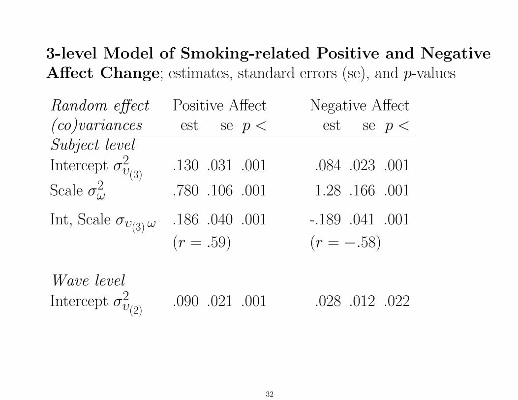
3-level Model of Smoking-related Positive and NegativeAffect Change; estimates, standard errors (se), and p-values

Random effect Positive Affect Negative Affect(co)variances est se p < est se p <Subject level

Intercept σ2υ(3)

.130 .031 .001 .084 .023 .001

Scale σ2ω .780 .106 .001 1.28 .166 .001

Int, Scale συ(3) ω .186 .040 .001 -.189 .041 .001

(r = .59) (r = −.58)

Wave level

Intercept σ2υ(2)

.090 .021 .001 .028 .012 .022

32

Mixed-effects Proportional Odds Model: ordinal responseYij of subject i (i = 1, 2, . . . , N) on occasion j (j = 1, 2, . . . , ni)

λijc = log

Pijc

1− Pijc

= γc −[x′ijβ + υi

]

Pijc = Pr(Yij ≤ c) cumulative probabilities for C categories of Y

xij = p× 1 vector of regressors (no 1 for the intercept)

β = p× 1 vector of regression coefficients

γ1 < γ2 < . . . < γC−1 strictly increasing thresholds

υi ∼ N(0, σ2υ) BS variance

33

Ordinal Response and Threshold Concept

Continuous yij - unobservable latent variable - related to ordinalresponse Yij via “threshold concept”

• threshold values γ1, γ2, . . . , γC−1 (γ0 = −∞ and γC =∞)

• C = number of ordered categories

Response occurs in category c, Yi = c if γc−1 < yij < γc

34

The Threshold Concept in Practice

“How was your day?”(what is your level of satisfaction today?)

• Satisfaction may be continuous, but we sometimes emit anordinal response:

35

Model for Latent Continuous Responses

Model with p covariates for the latent response strength yij:

yij = x′ijβ + υi + εij

where υi ∼ N(0, σ2υ), BS variance, and WS errors

• εij ∼ standard normal (mean 0 and σ2ε = 1)

mixed-effects ordinal probit regression

• εij ∼ standard logistic (mean 0 and σ2ε = π2/3)

mixed-effects ordinal logistic regression

36

Mixed-effects Ordinal Location Scale Model

λijc =γc − (x′ijβ + υi)

σεij

BS variance σ2υij = exp(u′ijα) or log(σ2

υij) = u′ijα

WS variance σ2εij = exp(w′ijτ + ωi) or log(σ2

εij) = w′ijτ + ωi

• uij and wij include covariates (and 1 only for ui)

• random location effects υi ∼ N(0, σ2υ)

• random scale effects ωi ∼ N(0, σ2ω)

37

Ecological Momentary Assessment (EMA) Study ofAdolescent Smokers (Mermelstein)

• 461 adolescents (9th and 10th graders); former and currentsmoking experimenters, and regular smokers

• Carry PDA for a week, answer questions when prompted

average = 30 answered prompts (range = 7 to 71)

• ∑Ni ni = 14, 105 total number of observations

Outcome: “I Felt Sad”

Interest: characterizing determinants of affect level, as well as BSand WS affect heterogeneity

38

I Felt Sad: marginal response frequencies and percentages

Sad Frequency Percent1 6087 43.152 2269 16.093 1716 12.174 813 5.765 439 3.116 671 4.767 773 5.488 579 4.109 292 2.07

10 466 3.30

⇒ items rated on 1 (not al all) to 10 (very much) scale

39

mean std dev min maxSubject-level independent variablesMale .449 .498 0 1Smoker .508 .500 0 1Psmk (234 smokers) .131 .117 .014 .583AloneBS .517 .196 .024 .950

Prompt-level independent variablesAloneWS 0 .461 -.950 .976

Smoker: gave at least one report of a smoking event in the week ofEMA measurement (about half of the subjects)

Psmk: proportion of occasions (random prompts and smoking events) thatwere smoking events = n smk / (n smk + n random)

For occasion-varying Alone, BS and WS decomposition:

Xij = X̄i + (Xij − X̄i)40

Proportional odds mixed modelestimates, standard errors (se), and p-values

parameter estimate se p <Male β1 -.716 .161 .0001Smoker β2 .477 .198 .017PSmk β3 -1.253 .942 .19AloneBS β4 1.082 .410 .009AloneWS β5 .527 .036 .0001BS variance α0 .965 .074 .0001

In terms of the BS variance, σ̂2υ = exp(.965) = 2.625

Intraclass correlation (ICC)ICC = 2.625/(2.625 + π2/3) = .44

41

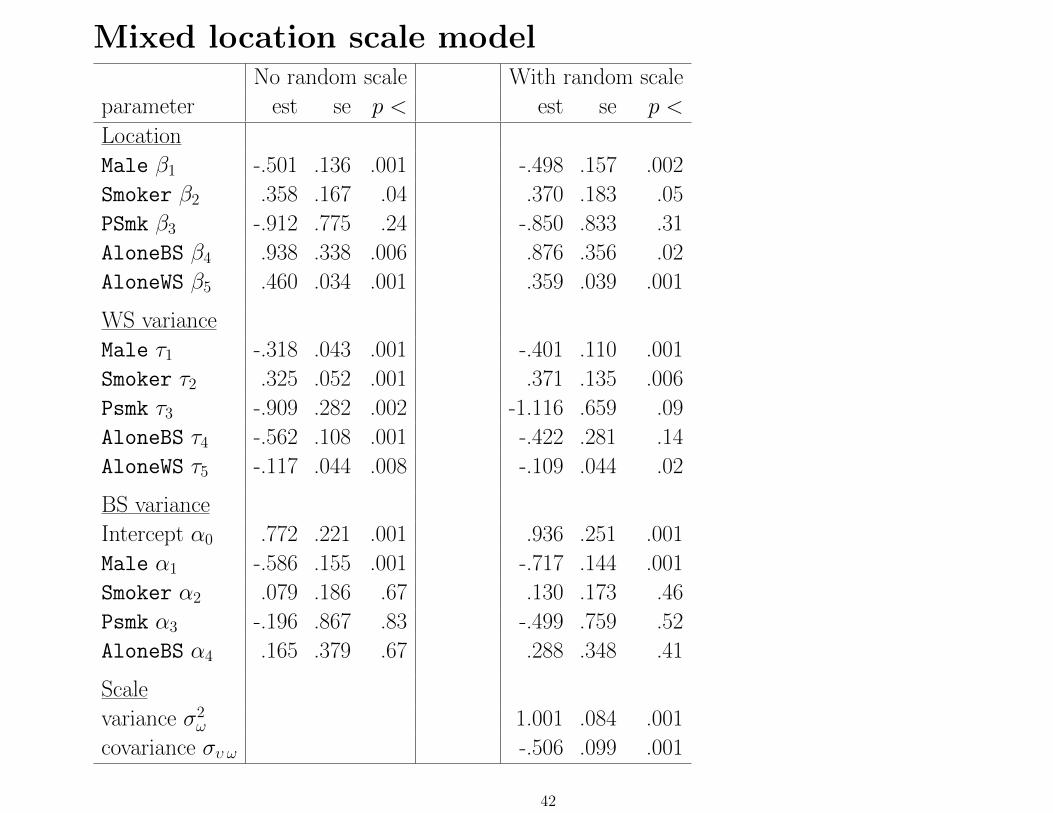
Mixed location scale modelNo random scale With random scale

parameter est se p < est se p <

Location

Male β1 -.501 .136 .001 -.498 .157 .002

Smoker β2 .358 .167 .04 .370 .183 .05

PSmk β3 -.912 .775 .24 -.850 .833 .31

AloneBS β4 .938 .338 .006 .876 .356 .02

AloneWS β5 .460 .034 .001 .359 .039 .001

WS variance

Male τ1 -.318 .043 .001 -.401 .110 .001

Smoker τ2 .325 .052 .001 .371 .135 .006

Psmk τ3 -.909 .282 .002 -1.116 .659 .09

AloneBS τ4 -.562 .108 .001 -.422 .281 .14

AloneWS τ5 -.117 .044 .008 -.109 .044 .02

BS variance

Intercept α0 .772 .221 .001 .936 .251 .001

Male α1 -.586 .155 .001 -.717 .144 .001

Smoker α2 .079 .186 .67 .130 .173 .46

Psmk α3 -.196 .867 .83 -.499 .759 .52

AloneBS α4 .165 .379 .67 .288 .348 .41

Scale

variance σ2ω 1.001 .084 .001

covariance συ ω -.506 .099 .001

42

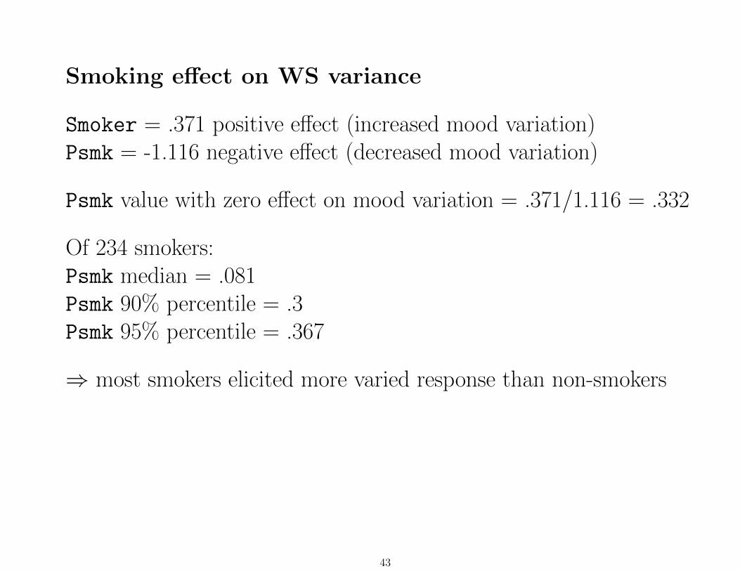
Smoking effect on WS variance

Smoker = .371 positive effect (increased mood variation)Psmk = -1.116 negative effect (decreased mood variation)

Psmk value with zero effect on mood variation = .371/1.116 = .332

Of 234 smokers:Psmk median = .081Psmk 90% percentile = .3Psmk 95% percentile = .367

⇒ most smokers elicited more varied response than non-smokers

43

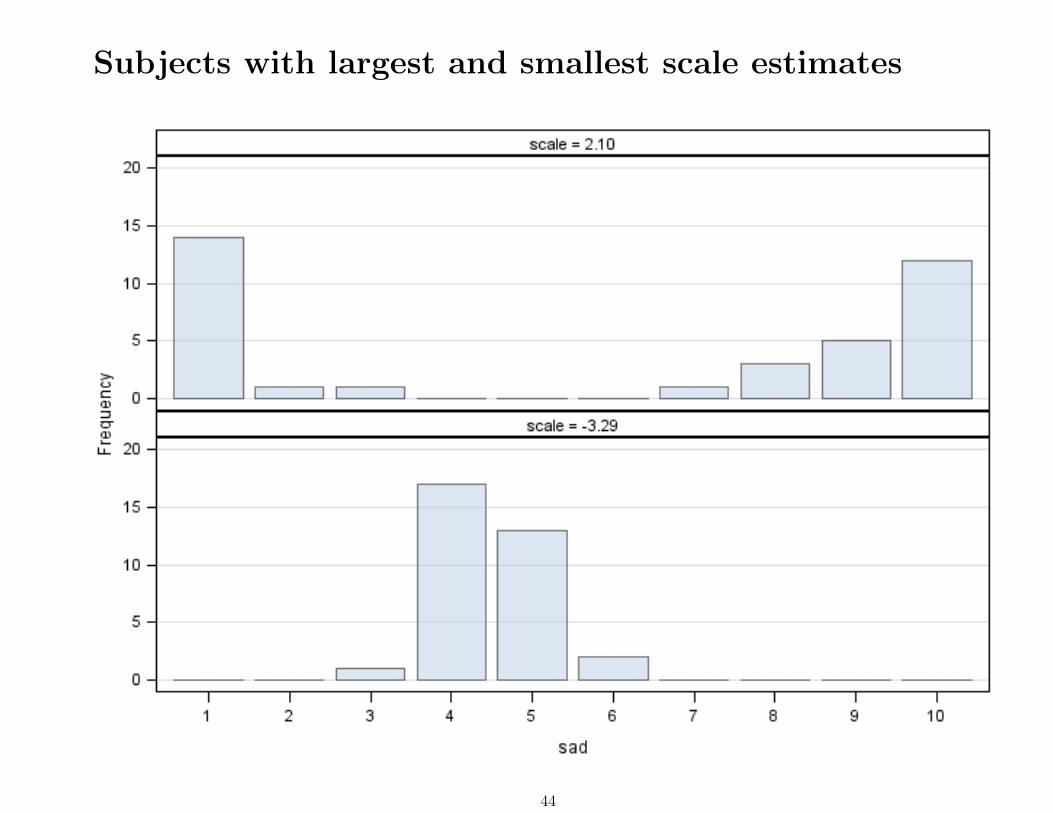
Subjects with largest and smallest scale estimates

44

Summary

•More applications where interest is on modeling varianceHedeker, D., Mermelstein, R.J., & Demirtas, H. (2008). An application of a mixed-effects location scalemodel for analysis of Ecological Momentary Assessment (EMA) data. Biometrics, 64, 627-634.

Hedeker, D., Mermelstein, R.J., & Demirtas, H. (2012). Modeling between- and within-subject variance inEMA data using mixed-effects location scale models. Statistics in Medicine, 31, 3328-3336.

Hedeker, D. & Mermelstein, R.J. (2012). Mood changes associated with smoking in adolescents: Anapplication of a mixed-effects location scale model for longitudinal EMA data. In G. R. Hancock & J.Harring (Eds.), Advances in Longitudinal Methods in the Social and Behavioral Sciences (pp. 59-79).Information Age Publishing, Charlotte, NC.

Hedeker, D. & Nordgren, R. (2013). MIXREGLS: A program for mixed-effects location scale analysis.Journal of Statistical Software, 52(12), 1-38.

Kapur, K., Li, X., Blood, E.A., & Hedeker, D. (2015). Bayesian mixed-effects location and scale modelsfor multivariate longitudinal outcomes: An application to ecological momentary assessment data.Statistics in Medicine, 34, 630-651.

Li, X. & Hedeker, D. (2012). A three-level mixed-effects location scale model with an application toEcological Momentary Assessment (EMA) data. Statistics in Medicine, 31, 3192-3210.

Pugach, O., Hedeker, D., Richmond, M.J., Sokolovsky, A., & Mermelstein, R.J. (2014). Modeling moodvariation and covariation among adolescent smokers: Application of a bivariate location-scalemixed-effects model. Nicotine and Tobacco Research, 16, Supplement 2, S151-S158.

• Ordinal outcomesHedeker, Demirtas, & Mermelstein (2009). A mixed ordinal location scale model for analysis of EcologicalMomentary Assessment (EMA) data. Statistics and Its Interface, 2, 391-402.

Hedeker, D., Mermelstein, R.J., Demirtas, H., & Berbaum, M.L. (under review). A mixed-effectslocation-scale model for ordinal questionnaire data.

45

More Examples of Variance Models in Health Studies

• Lin, Raz, & Harlow (1997) Linear mixed models with heterogeneous within-cluster variances,

Biometrics. Determinants of menstrual cycle length variability in women (which may be

associated with fertility and long-term risk of chronic disease).

• Carroll (2003) Variances are not always nuisance parameters, Biometrics. Drug assay

validation, measurement error in nutrient intake.

• Elliott (2007) Identifying latent clusters of variability in longitudinal data, Biostatistics.

Clusters based on within-subject variation in affect of recovering MI patients.

• Elliott, Sammel, & Faul (2010) Associations between variability of risk factors and health

outcomes in longitudinal studies, Statistics in Medicine. Residual variability in longitudinal

recall data associated with dementia risk in elderly.

• Rast & Zimprich (2011) Modeling within-person variance in reaction time data of older adults,

Journal of Gerontopsychology and Geriatric Psychiatry.

• Coffman, Allen, & Woolson (2012) Mixed-effects regression modeling of real-time momentary

pain assessments in osteoarthritis (OA) patients, Health Services and Outcomes Research

Methodology. Pain variability in patients with osteoarthritis.

• Breslin (2014) Five indices of emotion regulation in participants with a history of nonsuicidal

self-injury: A daily diary study, Behavior Therapy.

46

• Need a fair amount of BS and WS data, but modern datacollection procedures are good for this. Also, from analysis ofRiesby depression data (N = 66, ni = 4 to 6):

The data of the two highest and lowest scale estimates from analysis of the Riesby data

id θ̃2i hd0 hd1 hd2 hd3 hd4 hd5

606 1.585 19 33 12 12 3 1505 1.532 21 11 18 0 0 4

335 −1.317 21 21 18 15 12 10308 −1.365 22 21 18 17 12 11

• Simulations with small datasets (e.g., 20 subjects with 5 obs)often leads to non-convergence; this improves dramatically asnumbers increase (e.g., 100 subjects with 10 obs)

• Important to include random scale for correct inference of WSvariance covariates (Leckie et al., 2014, Jrn Educ Beh Stat)

47