DI

SC

US

SI

ON

P

AP

ER

S

ER

IE

S

Forschungsinstitut zur Zukunft der ArbeitInstitute for the Study of Labor

Does the Sector Experience Affect the Pay Gap for Temporary Agency Workers?

IZA DP No. 5837

July 2011

Elke JahnDario Pozzoli

Does the Sector Experience Affect the

Pay Gap for Temporary Agency Workers?

Elke Jahn IAB, Aarhus University and IZA

Dario Pozzoli

Aarhus University

Discussion Paper No. 5837 July 2011

IZA

P.O. Box 7240 53072 Bonn

Germany

Phone: +49-228-3894-0 Fax: +49-228-3894-180

E-mail: iza@iza.org

Any opinions expressed here are those of the author(s) and not those of IZA. Research published in this series may include views on policy, but the institute itself takes no institutional policy positions. The Institute for the Study of Labor (IZA) in Bonn is a local and virtual international research center and a place of communication between science, politics and business. IZA is an independent nonprofit organization supported by Deutsche Post Foundation. The center is associated with the University of Bonn and offers a stimulating research environment through its international network, workshops and conferences, data service, project support, research visits and doctoral program. IZA engages in (i) original and internationally competitive research in all fields of labor economics, (ii) development of policy concepts, and (iii) dissemination of research results and concepts to the interested public. IZA Discussion Papers often represent preliminary work and are circulated to encourage discussion. Citation of such a paper should account for its provisional character. A revised version may be available directly from the author.

IZA Discussion Paper No. 5837 July 2011

ABSTRACT

Does the Sector Experience Affect the Pay Gap for Temporary Agency Workers?*

It is a well-known fact that temporary agency workers have to accept high pay penalties. However, remarkably little is known about the remuneration of workers who are frequently employed in this sector or who are employed for a substantial length of time. Based on a rich administrative data set, we estimate the effects of the intensity of agency employment on the temp wage gap and post-temp earnings in Germany. Using a two-stage selection-corrected method in a panel data framework, we show that the wage gap for temps with low treatment intensity is high but decreases with exposure to the sector. It seems that temps are able to accumulate human capital while being employed in this sector. Temps who move to permanent jobs have to accept a sizeable wage disadvantage at first, indicating that temporary agency employment might stigmatise workers. However, agency employment does not seem to leave a long-lasting scar. JEL Classification: J30, J31, J42, J41 Keywords: temporary agency employment, treatment intensity,

dose response function approach, wages, Germany Corresponding author: Elke Jahn Institute for Employment Research (IAB) Regensburger Straße 148 90478 Nuremberg Germany E-mail: elke.jahn@iab.de

* We would like to thank Sylvie Blasco, Nabanita Datta Gupta, Boris Hirsch, Marie Paul, Regina T. Riphahn, Michael Rosholm, Claus Schnabel, Gesine Stephan, the participants of the IAB/LASER workshop “Increasing Labor Market Flexibility - Boon or Bane?” in March 2011 and the participants of the ASB/IAB workshop “Labor Markets and Trade in a Changing World” in May 2011 for helpful comments and suggestions.

1 Introduction

Investigating the working conditions and the remuneration of temporary agency workers

has become increasingly important as temporary agency employment has become a signif-

icant employment form in most OECD countries during the past decades.1 This trend has

particularly been observed in Western Europe and Japan. Germany, together with the

US and the UK, has become one of the largest markets in the world (CIETT, 2011). As

temporary agency jobs are often regarded as bad jobs, the expansion of this sector raises

concerns about labour market segmentation that traps particularly low-skilled workers in

jobs providing few career prospects and poor pay.

The empirical evidence for European countries indeed indicates that the average wage

of agency workers lags behind that of permanent workers. As a consequence, not only

most European governments but also the European Commission feel the need to intervene.

For example, the European Parliament approved a directive which stipulates equal pay

for permanent and agency workers in 2008. From 2012 onwards, member states can only

deviate from the principle of equal treatment if workers are paid either by a collective

agreement or by an agreement between the national social partners (Eurofound, 2008).

However, the literature so far has concentrated on the temp wage gap, neglecting the

fact that agency employment is a rather heterogenous phenomenon. While some workers

accept only one agency job during their employment career, for others it might be a

career choice, as they repeatedly accept temp jobs or are employed in this sector for a

considerable length of time. The latter group particularly may not perceive agency work

as flexible and unstable. On the contrary, their jobs might be more similar to regular

jobs.

1To ease readability, we use the terms temp job or agency employment interchangeably with temporaryagency employment and temp or agency worker instead of temporary agency worker.

1

The purpose of this article is to gather new evidence for Germany by estimating not

only the wage differentials between temp and non-temp workers as in previous literature,

but also to take into account the heterogeneity of this employment form. Perceiving

temp employment as a multi-valued treatment allows us to test directly whether higher

exposures to temporary agency employment result in an improvement in or a deterioration

of wages in the temp sector or in post-temp employment.

One of the most difficult issues in the literature is to control for self-selection of workers

by unobserved individual traits, like ability (Autor 2009). If one does not take into

account the individual’s endogenous contract decision, observed market wages for different

doses may still be the result of selection, even after controlling for individual worker and

job characteristics. In this case, parameter estimates might be inconsistent and biased

either upwards or downwards. To address the issue of selection into temporary agency

employment, in this paper we apply a two-stage selection-corrected method in a panel

data framework, using a rich administrative data set for Germany covering the period

2000-2008.

This study adds to the literature in this field in several respects. To the best of our

knowledge, this is the first time that a dose-response function approach has been applied

within a panel data setting. Second, combined with a suitable IV-type identification strat-

egy, our econometric model allows us to fill a gap in the literature by providing evidence

on the causal impact of agency employment intensity on wages. Third, to assess whether

agency workers are stigmatised once they leave the sector, we implement a propensity

score matching estimator to compare wages of workers who have been exposed to agency

employment in different ways with wages of individuals without agency experience.

Our estimations show that the wage gap decreases with the time a worker spends

2

in the sector at the same job or with different employers, after having controlled for

time invariant unobserved heterogeneity and self-selection. This indicates that workers

are able to accumulate human capital in the agency sector which pays off in terms of

remuneration. Temps who move to permanent jobs have to accept high pay differentials

at first, indicating that agency employment might stigmatise workers. However, agency

employment does not leave a long-lasting scar. After being employed for four quarters

outside the sector, all workers will have caught up to workers employed outside the sector.

The paper is organised as follows. Section 2 provides some background information on

temporary agency employment and presents the main hypothesis. Section 3 highlights key

facts about the temporary employment sector in Germany. Section 4 introduces the data

set and presents main descriptive statistics. Section 5 provides details on the empirical

strategy. Section 6 explains the results of our empirical analysis and Section 7 concludes.

2 The Debate on Temporary Agency Employment

Poor working conditions and the disproportionate concentration of disadvantaged workers

in the temporary employment sector are the main reasons why agency employment is of

key interest in the policy debate on labour market flexibility. Studies on the stepping stone

effect of agency employment stresses the acquisition of human capital as the main channel

through which agency employment can be a pathway to regular jobs (e.g. Abraham,

1990). The argument is that temporary agency work may not only improve workers’

human capital, due to their training within the sector and various assignments, but agency

workers might even be able to acquire more human capital than workers employed in other

sectors for a given period of time (Autor, 2001). Critics of this argument, however, claim

that these human capital effects cannot be strong, given the short job duration, low-skilled

3

content and low match quality (Segal and Sullivan, 1997).

So far the question of whether temp workers can indeed gain valuable skills which

ease the transition to regular employment has been an open one. While some studies find

that agency employment improves subsequent employment outcomes (Ichino et al., 2008;

Lane et al.,2003; Jahn and Rosholm, 2010), others find no evidence for the stepping stone

function of agency work (Amuedo-Dorantes et al., 2008; Autor and Houseman, 2011; De

Graaf-Zijl et al. 2011; Garcıa-Perez and Munoz-Bullon, 2005; Kvasnicka, 2009; Malo and

Munoz-Bullon, 2008). This literature suggests that for some unemployed people agency

jobs might be the only way to participate in the labour market. Therefore, the question

arises whether working in this sector can still have some benefits in terms of earnings.

Theoretically, the size of the temp wage gap is not clear cut: The theory of compen-

sating wage differentials claims that a competitive labour market rewards poor working

conditions (Rosen, 1986), such as a higher risk of unemployment. However, there are also

arguments justifying why temps should have to accept a wage penalty. First, temporary

agency employment has features of an investment. If agency workers can improve their

skills, than human capital theory would suggest that workers should also have to bear

the cost by accepting lower wages while employed in this sector (e.g. Becker 1964). Sec-

ond, temps may also gain from the placement activity of the labour market intermediary,

which decreases their search costs and improves match quality. The wage penalty can

then be seen as a compensation for this service (Jahn, 2010, Neugart and Storrie, 2006).

Third, compared to workers in other sectors temps may be less productive as they are less

motivated, invest less in firm-specific human capital, and are often employed below their

qualifications (Houseman et al., 2003). Finally, as Blank (1998) and Ransom and Oaxaca

(2005) point out, most workers accept agency jobs because of a lack of alternatives. This

4

might provide the basis for labour market segmentation as agencies are able to exercise

monopsony control over the wages of workers with low bargaining power. The empirical

evidence for continental European countries indicates that the average wage of temporary

agency workers lags behind those of permanent workers by between 2 percent in Portugal

(Boheim and Cardoso, 2009) and 15 percent in Germany (Jahn, 2010). However, the

temp wage gap is not only a continental European phenomenon. The results provided by

Segal and Sullivan (1998) and Addison et al. (2009) for the US, Booth et al. (2002) and

Forde and Slater (2005) for the UK and Cohen and Haberfeld (1993) for Israel confirm

that temps in those countries also have to accept a considerable wage penalty.

Regarding the size of the post-temp earnings, there are two main competing hypothe-

ses: Autor (2001) stresses that due to training inside the sector, agency workers might be

able to accumulate more human capital than their counterparts outside the sector. Such

training may result in an increase in wage in post-temp jobs. Alternatively, one might

argue that temp workers may be stigmatised in the sense that future employers may

perceive a previous temp job as being an indicator of a worker’s lower ability and motiva-

tion. This negative signal might result in fewer job offers and job offers with lower wages

than other workers would receive (Blanchard and Diamond, 1994). Regarding post-temp

wages, there are few studies available for the US which indicate that an unemployed per-

son accepting an agency job might be stigmatised as they have to accept lower, long-run

earnings than those who exit directly from unemployment to regular work (Andersson et

al., 2009; Autor and Houseman, 2011; Heinrich et al., 2009).

All studies on the relative earnings of agency workers so far assume that the agency

market is homogenous and have therefore focused on binary definitions of treatment.

However, if one looks at the duration of agency jobs and the number of agency jobs workers

5

accept during their employment career, it becomes apparent that agency employment is

a rather heterogeneous form of employment. While some workers accept agency jobs on

a regular basis and for a considerable length of time, other workers experience only one

temp job during their employment career. This heterogeneity of agency work compared

to other flexible employment forms like fixed-term contracts results from the numerous

motives as to why workers accept agency employment or why firms fall back on it.

We argue that the resulting variety in duration and the number of jobs accepted in the

sector manifest themselves in the temp wage gap. If agencies provide workers with free

training and agency workers are able to improve their human capital while assigned to

different employers, one might suspect that the wage gap for workers with an employment

career within the sector might be smaller or even dissipate. In this case longer agency

experience might be of equivalent value to an employment career outside the sector and

concerns about the quality of agency jobs may be unfounded for at least one part of the

flexible staff. On the other hand, if agency workers are employed below their skill level,

they will not be able to improve their human capital. It may even depreciate and agency

work may stigmatise workers. In this case, more exposure to the sector may deteriorate

current and future wages and agency employment may even foster the development of

dual labour markets in which low-wage workers move from one bad job to the next.

The intensity of temp experience may also affect post-temp wages. One would expect

that workers with low treatment intensities might not have had enough time or have

received any training, so that the interim job signals low ability and does not pay off.

Workers with higher exposure to agency employment, however, might be able to transfer

their work experience and human capital to jobs outside the sector. In this case it is

plausible to assume that these temps may also gain in terms of remuneration after leaving

6

the sector.

The exposure to agency employment depends inter alia on the motive for accepting

an agency job. Due to preferences for home production, flexible contracts might more

often be a career choice for women than the result of a lack of alternatives. Therefore,

it might be optimal for female workers to invest in general rather than specific human

capital and also to accept multiple agency jobs (Booth et al., 2002). We therefore expect

that longer experience in the sector or multiple temp jobs might affect female temps

differently. Their acquired human capital and flexibility might even be valued by firms

in terms of wages. Moreover, male temps are predominantly employed in the production

sector, where they accumulate firm or industry-specific human capital. This knowledge

can often not be transferred to other employers or between industries. Female temps,

however, are much more often assigned to office work and clerical jobs, where general

human capital is accumulated and can be transferred to a greater extent. Consequently,

we expect smaller temp wage gaps for women and also expect agency employment not to

harm or stigmatise this group of the labour force.

3 Temporary Agency Work in Germany

In Germany, agency employment is regulated by national legal statutes which only ap-

ply to temporary employment agencies. Compared to international standards, agency

employment was highly regulated until the end of 2003 (see Antoni and Jahn, 2009, for

details). In contrast to many other countries where temps are exempted from compulsory

social benefits, all workers in Germany have access to health insurance, holiday leave and

pension plans. Agency workers with a permanent employment contract lasting more than

six months are protected against dismissal by the rather strict employment protection

7

legislation. Consequently, temp workers are rarely employed for more than six months at

the same agency. Instead, they often move from one temp agency to the next.

The most recent reform, which came into effect in 2004, was intended to strengthen

the rights of temp workers by applying the principle of equal pay from the first day of

an assignment. The new law allows deviation from the principle of equal treatment if

the agency applies the conditions stipulated in a collective agreement to all its workers.

Therefore, wage gaps between temps and the permanent staff of a user firm are permissible

if the wages established in the user firm’s collective agreement are higher than those in

the temp industry’s collective agreement. In addition, by signing a collective agreement,

the agency can free itself of all other regulations. As a consequence, numerous collective

agreements were concluded in anticipation of this reform. By the end of 2003, nearly 97

percent of the agencies were paying their temps according to a collective agreement and

the principle of equal treatment and all other regulations have since lost any practical

meaning for the temporary employment industry.2

During our observation period, the share of agency workers increased tremendously.

In 2000, temporary agency employment constituted about one percent of the wage and

salary workforce. In 2008, about three percent of workers were employed in this sector. As

most temp jobs in Germany are full-time jobs, temps rarely hold multiple jobs. Blue-collar

occupations such as jobs in production, labourers and other low-skilled jobs are dominant

in this sector. The concentration of low-skilled workers in this sector in combination

with the assertion that the German metal industry (e.g. the automobile, shipping and

aircraft industries) uses temps to circumvent the high wages in the metal sector’s collective

agreements is one main reason why the remuneration of agency workers is of key interest

2However, Jahn (2010) has shown that this reform had no effect on the size of the temp wage gap.

8

in the German policy debate.

4 Data

4.1 Data Description

Our empirical analysis is based on a 5 percent random sample of temporary agency work-

ers and a 0.5 percent sample of remaining workers drawn from the Integrated Employment

Biography (IEB). The IEB contains daily information about employment periods subject

to social security contributions, unemployment periods, and socio-economic and job char-

acteristics at the individual level (see Dorner et al., 2010). Being of administrative nature,

the IEB also provides longitudinal information on the employment history. The IEB is

especially useful for analyses taking wages into account, since the wage information is

used to calculate social security contributions and is therefore highly reliable.

The daily wage, which is used in this analysis, is calculated by dividing the reported

earnings by the duration of the notification period in calendar days. Employers report the

gross earnings of their employees for the period in which the worker has been employed,

but at least once at the end of a year. This means that for longer spells changes in earnings

might be visible only at the beginning of the next calendar year. Moreover, as the median

job duration of temp workers is below 12 weeks this should only bias slightly downwards

our results for lower levels of exposure. Agencies have a high incentive to dismiss the

temp as soon as the assignment ends. Based on a panel data set of one of the largest

temporary employment agencies in Germany, Kvasnicka (2003) provides evidence that

the majority of temp workers have only one assignment, agencies rarely bridge periods

without assignment, and the number of actual hours worked on average slightly exceeds

9

that agreed contractually. Consequently, it is unlikely that differences in earnings will

be a consequence of the fact that temp workers only receive a basic wage during periods

without an assignment or that the number of hours worked weekly will be below the

number of hours contractually agreed.

Wages above the social security contribution ceiling are top-coded. To address this

issue we imputed top-coded wages using the heteroscedastic single imputation approach

developed by Buttner and Rassler (2008) for an earlier version of this data set. However,

as agency jobs are typically low-paid jobs, top-coding should not affect our results.3

Nevertheless, the IEB has some minor drawbacks. First, employment spells in tempo-

rary employment agencies are identified by an industry classification code. Consequently,

agency workers cannot be distinguished from agencies’ administrative staff, which ac-

counted for about five to seven percent of agency employees in 2003, depending on the

size of the agency (Antoni and Jahn, 2009). Note also, as the legal employer is the agency,

we do not observe how often and in which sectors a worker has been assigned.

Second, the IEB does not provide information on hours worked. We therefore exclude

part-time employees, interns and home workers from the sample since the wage infor-

mation is not comparable for these groups. As 91 percent of the temp workers during

our observation period were employed full-time, this decision should not affect our main

results. Trainees are excluded from the analysis as they are part of the agency staff.

Third, the information on education is provided by employers and is missing for about

19 percent of the employment spells. We therefore imputed the missing information

on education by employing a procedure developed by Fitzenberger et al. (2005) for an

earlier version of this data set, which also allows inconsistent information on education to

3As a robustness check we ran all estimations without imputed wages. It turns out that the tempgaps were only negligibly smaller.

10

be corrected over time. After applying this imputation procedure, we had to drop about

4 percent of the spells due to missing or inconsistent information on education.

The analysis is restricted to the period from 1995 to 2008 and to non-agricultural

employees between the ages of 18 and 60. We used the information for the 1995 to 1999

period to control for the employment career of the workers in the previous five years.

This allows estimating the wage equations for the 2000 to 2008 period. To estimate the

wage differentials, we constructed a quarterly panel data set, but we took advantage of

the daily spell structure to construct the workers’ employment history.

4.2 Variables and Descriptive Statistics

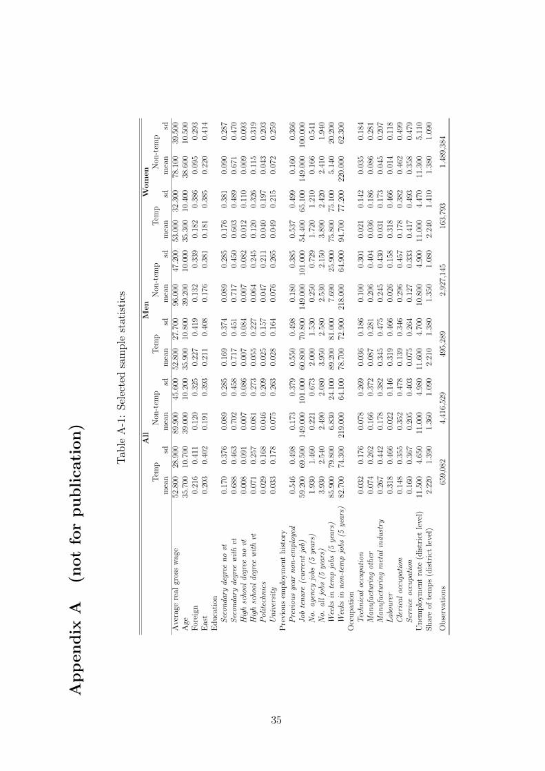
In our analysis we include 5.1 million spells, among them 659 thousand temp spells (see

Table 1). About 75 percent of the temps are male. The dependent variable is the log

gross daily wage of the worker, which has been deflated to 2005 levels using the CPI

deflator. Agency workers earn less than regular workers. The mean daily real gross wage

is 53 euros for temp workers and 90 euros for regular workers. In order to get a first idea

of the temp wage gap, we run OLS regressions by gender, which include only a dummy

for being a temp worker as a control. The first striking result is that the raw temp wage

gap is about 50 percent. Table 1 also reveals that the wage differential for women is

considerably smaller than that for men.

The multi-valued treatment is measured either as the number of agency jobs or the

cumulative number of weeks in temporary agency employment over the past five years.

The latter group of treatment indicators allows that workers switch agencies or have had

a period of regular employment in between.

Table 1 informs about the number of observations by treatment dose. Depending on

11

gender, about 53 percent of the agency spells show a previous temp experience of more

than 52 weeks and 15 percent an exposure of less than 12 weeks. However, the calculations

in Table 1 are cumulating the temp experience over the past five years. In practice, agency

jobs are rather short. About 50 percent of the agency jobs lasted for fewer than 12 weeks;

20 percent lasted between three and six months, 14 percent of the jobs had a duration

of between six months and one year, and another 16 percent lasted longer than one year.

Regarding the number of agency jobs, Table 1 reveals that 54 percent of the spells show

experience of only one temp job and about 11 percent had more than three agency jobs.

Table 1 also reveals that the employment career of temp workers is much more frag-

mented. On average, they changed jobs about four times and accepted two temp jobs five

years prior to their current temp job. In contrast, workers who are currently employed

outside the temporary employment sector switched jobs twice and barely have any temp

experience.

As socio-demographic controls the following variables are included: gender, age, age

squared, citizenship and education (six classes). The employment history is controlled for

by a dummy indicating whether or not the worker has experienced a period of unemploy-

ment or not being part of the labour force during the past 12 months, the number of jobs

during the past five years, the regular employment experience in weeks during the past

five years and its square, and job duration in weeks and its square. As far as the current

job is concerned, we differentiate between six occupational groups (see Jahn, 2010, for

more details).

To account for the heterogeneity among the agencies, we include the age of the firm,

the firm size (five classes), the share of female workers in the agency, the percentage of

employees with a university degree, and the share of workers with no vocational training.

12

Finally, as macroeconomic variables, we include the real annual growth rate of GDP,

the quarterly, regional unemployment rate (based on 413 districts), a dummy for East

Germany and three variables indicating whether a worker is employed in a metropolitan,

urban or rural area.

The average age of temp workers (36) is lower than in the comparison group (39).4

Workers without vocational training are overrepresented in temp employment (18 per-

cent), compared to their share in regular employment (10 percent). In contrast to most

European countries, service jobs and clerical occupations do not play an important role.

More than two-thirds of male temps are employed in manufacturing or as labourers.

Women more often work in clerical and service occupations. While about 55 percent of

the temps were unemployed during the past 12 months or were not part of the labour

force, this is only true for 17 percent of the non-temps.

5 Empirical Strategy

5.1 Wage Gap of Temporary Agency Workers

This section describes a consistent estimation procedure for the generalised sample selec-

tion model with panel data. The point of departure is the following endogenous switching

model:

w0it = α0

0 + X′itα

01 + µ0

i + τt + ε0it for t0i s.t. Dit = 0

w1it = α1

0 + X′itα

11 + µ1

i + τt + ε1it for t1i s.t. Dit = 1

(1)

4Selected sample statistics can be found in the Appendix and are available on request from the authors.

13

where wit is the log of the real daily wage for worker i in quarter t, X is a vector

of the observed worker and job characteristics described in the previous section, µ are

the time-invariant individual specific effects and τ includes the GDP growth rate, the

unemployment rate and a full set of quarter and year dummies. The binary indicator D

is the endogenous treatment variable, which is defined according to the following binary

response model:

D∗it = β0 + Z′

itβ2 + ηi + vit (2)

where the vector Z includes both a set of worker characteristics5, as age and education,

and the current value and the time mean of the shares of temporary agency workers at

district level, the latter being our exclusion restrictions. The districts are clusters of

municipalities, which are grouped based on commuting patterns that can be interpreted

as self-contained labour markets. In total, 413 local labour markets are identified. In

our opinion, they represent a more appropriate territorial configuration for examining the

interaction between workers and potential externalities than larger administrative areas,

such as federal states . The share of agency workers at the district level proxies the

local concentration of temporary work agencies and represents a suitable instrument for

the individual decision to be an agency worker which is not correlated with earnings. It

can be reasonably assumed that the share of agency workers within the commuting area

strongly influences the probability that a recently dismissed or unemployed individual,

for example, will end up being a temp, but that it will barely affects her wages.6

5Results obtained from using alternative specifications of the selection equation are qualitatively sim-ilar to those reported in the paper and are available on request.

6Note that we are able to exploit variation over time and district level: The average share of agencyworkers during our observation period is 1.5 percent; the regional interdecile range is 2.8 percent (firstdecile 0.2 and ninth decile 3.0 percent).

14

Following Mundlak (1978), we assume that the conditional expectation of the individ-

ual specific effects in the selection and the wage equation, µi and ηi, are linear in the time

means of variables included in the vector Z.

In the equations of interest we should take into account that when cov(εkit, vit) 6= 0,

then neither E(ε0it|s∗it ≤ 0) or E(ε1it|s∗it > 0) is expected to be zero. In order to control for

the endogenous selection problem, we estimate the parameters of the indicator equation

(2) and then, under the assumption of normality, which is not a crucial assumption for

the results to hold, we correct the equations of interest with corresponding time-varying

inverse Mills ratios or control functions.7 The control functions allow us to fully account

for the dependence of the time-varying, unobservable determinants of wages on the sector

assignment. Adding consistent estimates of the inverse Mills ratios, λ0i and λ1

i to equation

(1), we obtain:

w0it = α0

0 + X′itα

01 + µ0

i + ˆσ0λ0it + τt + e0

it for t0i s.t. Dit = 0

w1it = α1

0 + X′itα

11 + µ1

i + ˆσ1λ1it + τt + e1

it for t1i s.t. Dit = 1

(3)

We consistently estimate equations (3) using the pooled OLS estimator (Wooldridge,

1995; Semykina and Wooldridge, 2010). The variance and covariance matrix of the two-

step estimator is adjusted for the replacement of λit with λit by bootstrapping the se-

quential two-step estimator. Note that under the structure imposed on the model, the

estimated coefficients of the time varying inverse Mills ratios are informative on the pres-

ence and direction of the selection process (σ0 for the selection on unobserved ability or

productivity and σ1 for the selection on the basis of their unobserved gain or of an un-

7Following Wooldridge (1995) and Semykina and Wooldridge (2010), we estimate a reduced-formquarter by quarter probit model for the agency employment decision.

15

observed component in the treatment effect). Specifically, in the presence of an exclusion

restriction, as in our case, the null of no selection on unobservables can be tested directly.

In the framework above, this simply amounts to a test of the null hypothesis that σ0 and

σ1 are zero.

Compared to a single equation approach, the control function model described above

allows the temp effects to be heterogeneous across individuals in both observable and

unobservable dimensions. We argue that the latter model is more appropriate as it allows

us to test whether temp agency workers’ characteristics, like education and experience, are

remunerated and priced differently compared to regular workers. Under the assumption

that agency workers are mismatched in terms of skills to tasks, we expect the coefficients

α1 in the system of equations (3) to be heterogenous between temps and regular workers.

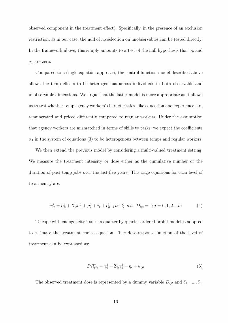
We then extend the previous model by considering a multi-valued treatment setting.

We measure the treatment intensity or dose either as the cumulative number or the

duration of past temp jobs over the last five years. The wage equations for each level of

treatment j are:

wjit = αj0 + X′

itαj1 + µji + τt + εjit for t

ji s.t. Dijt = 1; j = 0, 1, 2....m (4)

To cope with endogeneity issues, a quarter by quarter ordered probit model is adopted

to estimate the treatment choice equation. The dose-response function of the level of

treatment can be expressed as:

DR∗ijt = γj0 + Z′

itγj1 + ηi + uijt (5)

The observed treatment dose is represented by a dummy variable Dijt and δ1, ....., δm

16

are cut-off points for the different treatment levels. Hence the probability of having

treatment level j becomes:

prob(Dijt = 1) = Φ(δj − γj0 − Z′

itγj1)− Φ(δj−1 − γj0 − Z

′

itγj1) (6)

where Φ is a standard normal cumulative probability density function. Let ψij = σveσv

be the covariance matrix of error terms between treatment dose choice and wage equations

and

λijt = E(uσu| δj−1−γj0−Z

′itγ

j1

σu< u

σu<

δj−γj0−Z′itγ

j1

σu

)=

φ(δj−1−γ

j0−Z′itγ

j1

σu)−φ(

δj−γj0−Z

′itγ

j1

σu)

Φ(δj−γ

j0−Z′itγj1

σu)−Φ(

δj−1−γj0−Z′itγj1

σu)

, 1 < j < m

(7)

be the expected value of the control function term. Then equation (4) can be rewritten

as:

wjit = αj0 + X′

itαj1 + µji + ψijλijt + τt + ejit for t

ji s.t. Dijt = 1; j = 0, 1, 2....m (8)

As before we estimate equation (8) using a two-stage estimator.

The estimation results obtained from the previous selection-corrected wage equations

are used to calculate the implicit wage differential between different doses of agency

employment. The corrected differentials can generally be expressed as:

cdj =1

N

N∑i=1

T∑t=1

[E(wjit|Dijt = 1)− E(wj−1

it |Dij−1t = 1)]

(9)

where N is the number of individuals, wjit and wj−1it are predictions from the wage

equation (8), after substracting the selection terms.

17

5.2 Post-Temp Wages

In the next step we analyse whether different doses of agency employment affect post-temp

wages. The fact that we only observe post-temp wages for those who find a job outside

the sector implies that we are estimating the post-temp wage differentials for a rather

selected sample of workers. The lack of a reliable exclusion restriction, which explains

the transition out of the temp sector but does not affect individual post-temp wages,

does not allow us to estimate the sample selection model described above and to uncover

causal impacts of doses of agency employment on post-temp wages. In the following, we

instead compare wages for individuals who are currently employed as regular workers but

have been differently exposed to the temp sector in the previous five years with matched

individuals who were never exposed to agency employment in our sample period. The

fact that a worker never worked as a temp might still be a consequence of unobserved

heterogeneity for which we are not able to control. This means that the results of the

matching approach should also not be interpreted as causal, but they allow us to assess

to a certain degree whether workers are stigmatised when they leave the sector.

Following Lechner (2001), we instead calculate post-temp wage differentials by apply-

ing a multiple treatment matching model, where the exposure to M mutually exclusive

treatments is denoted by an assignment indicator D, D ∈ (0, ...,M). In our case, we as-

sume that an individual is observed in five alternatives D ∈ (0, ..., 4), which corresponds

to the levels of exposure to the agency sector as described in the previous sections. Lets

denote X as the set of matching variables8 and (W 0, ...,W 4) as the post-temp wages for

each level of previous exposure to the temp sector. Each individual is observed in one of

the treatments, therefore for each level of exposure only one component of (W 0, ...,W 5)

8The set of matching variables consists of the observed worker and job characteristics included in thewage equations of the main analysis.

18

can be observed in the data. The focus is on a pairwise comparison between the post-temp

wages of the treatment group m, with m 6= 0, compared to wages of the control group m,

with m = 0. More formally, the outcome of interest is:

θm0 = E(Wm −W 0|D = m) = E(Wm|D = m)− E(W 0|D = m) (10)

where θm0 denotes the expected average wage differential between individuals differ-

ently exposed to the temp sector before moving to the regular sector and those who have

never been exposed to the temp sector. The evaluation problem is a problem of miss-

ing data: one cannot observe the counterfactual E(W 0|D = m) since it is impossible

to observe the same individual in several states at the same time. Thus, the true wage

differential between the two groups can never be identified. However, the average wage

differential described by equation (10) can be identified under the conditional indepen-

dence assumption (CIA). To identify and estimate θm0, first of all we identify and estimate

E(Wm|D = m) by the sample mean. Exploiting the balancing property (Rosenbaum and

Rubin, 1983) and the CIA, we identify E(W 0|D = m) as follows:

E(W 0|D = m) = E[E[(W 0|Pm(X), D = 0)|D = m] (11)

where Pm is the probability that an individual with the set of characteristics X has

cumulated a certain level of work experience or number of jobs in the temporary employ-

ment sector before moving to the regular sector.9 For each level of previous exposure to

9The results reported in the paper are based on the propensities estimated from standard binomialmodels. One shortcoming of this approach may be that in each model only two treatment levels at atime are considered and consequently the choice is conditional on being in one of the two selected groups(Bryson et al., 2002). As a robustness check, we have also estimated the propensity scores from anordered probit and we have implemented a pairwise matching procedure based on the minimization ofthe mahalanobis distance of the corresponding vector of propensities (Imbens, 2000). The results arequalitatively similar to those discussed in the paper and are available on request.

19

the temp sector, the pairwise matching procedure is carried out four times: for the first,

second, fourth and eighth quarter after transition without any interruption by a temp job

in between.10 To avoid earnings of the control group being influenced by previous temp

jobs, we only select workers who had no agency experience during the observation period.

Both the control and treatment group are allowed to be unemployed or out of the labour

force between the observations as these periods are likely to affect wages of both groups

in the same way and these kinds of interruptions are controlled for by the employment

history.11

6 Results

6.1 Temp Pay Gaps

The estimated average treatment on the treated effects (ATT) from the control func-

tion model with endogenous switching is summarised in Table 2 for both the binary and

multi-valued treatments. In line with with the descriptive evidence, a negative effect of

temporary agency employment on wages is estimated. Interestingly, the earnings gap

decreases to about 20 percent for men and to 14 percent for women once the selection

on unobservables is taken into account. Binary treatment estimates also indicate that

women have to accept a considerably lower wage penalty.12 Table 3 shows that the selec-

tion adjustment terms or the standard inverse Mills ratios for both sectors are generally

10Each individual in the treated sub-sample m is matched with a comparison in the control group andthe criterion for finding the nearest possible match is based on a maximum propensity score distance(caliper) equal to 0.0001.

11As a robustness check, we have also estimated the post-temp wage differentials focusing on workerswho are employed in the regular sector for at least eight consecutive quarters. All in all, the results arequalitatively similar to those reported in Table 4.

12We ran all models separately for East and West Germany and for the pre- and post-reform period.Wage gaps in East Germany are slightly smaller than in West Germany. The same holds for the post-reform period. The full set of regression coefficients for each group is available from the authors.

20

significant and suggest a negative selection bias.13 This implies that the estimated wage

penalty is upward biased if the sample selection bias is not controlled for.

As pointed out in Section 5, the single equation approach assumes that agency em-

ployment affects all individuals equally. The endogenous switching model relaxes this

assumption and allows the effect to be heterogeneous in both observable and unobserv-

able characteristics. Table 3 presents the estimated wage equations for the treated and

non-treated separately. The coefficients on most of the observable characteristics differ

considerably across temp and non-temp workers. If we look at the education variables, for

example, it is immediately apparent that the regression coefficients imply very different

magnitudes depending on the employment contract. These findings warn against uncriti-

cal aggregation by sector and indicate the presence of observable heterogeneity, which we

need to take into consideration when the relevant treatment effects are estimated. All in

all, the results reported in Table 3 stress the need to allow for observable heterogeneous

returns in addition to selection on unobservables in our application.

Table 2 also summarises the estimated effects of the multi-valued treatments. If the

treatment is measured in weeks spent in agency employment over the last five years, we

find evidence that the estimated earning gaps decrease with treatment intensity.14 A male

temp worker who acquires more than 52 weeks of agency employment has a negative wage

gap of about 19 percent compared to a regular worker. The wage penalty rises to about

28 percent if a temp worker with fewer than 12 weeks of agency employment is considered.

Women with low temp experience also have to accept a surprisingly high wage differential

13As mentioned before, the current value and the time mean of the shares of temps at the district levelwhere individuals works are used as instruments. Besides the economic motivation for the instrumentspresented above, their statistical validity is largely confirmed by the F-statistics. The F-statistics arealways above 70, which allow us to clearly reject the null of weak instrument (Stock and Yogo, 2005).

14The detailed estimation results are available from the authors. In alternative specifications, we alsolook at the number of weeks spent in the current temp job. Results are qualitatively similar to thosereported in the paper.

21

of about 26 percent. However, considerably lower temp wage differentials are estimated

for women with more than 52 weeks’ temp experience. They have to accept a pay penalty

of about six percent only.

When we look at the number of temp jobs as treatment, only small differences in

the wage penalties are found across different numbers of treatments for men. Women,

however, even benefit from multiple temp jobs. Their wage gap decreases from 19 percent

if they have received one treatment to seven percent after having received at least four

treatments. Our results point out that agency workers are able to gain or improve their

human capital while being assigned which leads to better wages. Multiple temp jobs also

do not seem to stigmatise workers, at least if they stay in the sector.

Why must temp workers still accept a sizable wage gap despite being employed as

temps for a considerable length of time? Client firms recruit agency workers as leave

replacements, buffer stock, or to react immediately to economic fluctuations. In these

cases, the probability of moving to permanent contracts is low and it might be rational

for temps to defer investments in specific human capital. Consequently, agency workers

could show lower productivity than those who start in regular jobs, even when taking

into account the endogeneity of the contract decision. Only if workers are aware that the

assignment may be of longer duration do they have an incentive to invest in firm-specific

human capital. This is particularly the case if they hope that the client firm will take

them on in the future.

A second explanation could be that most temps work in the metal industry. The

metalworkers’ union is the largest and most powerful in Germany and wages there are

particularly high compared to other industries. The temporary employment industry

presents a stark contrast. Collective agreements have only played a role since the reform

22

in 2003. However, the main purpose of these agreements was to avoid the principle of equal

pay, and unions in this sector are rather weak. To investigate this issue we estimated the

wage gaps after excluding those working in the metal industry according to the industrial

classification code. Interestingly, the treatments measuring both the temp exposure in

weeks and the number of jobs drop for all treatment doses by about 4 percent for men

and 2 percent for women.

One reason why the wage gap for men reacts less strongly to the treatment intensity

could be that men are able to transfer accumulated human capital between different

employers to a lesser extent. It seems that the work experience they gain is more firm

or industry specific. Women, however, work more often as white-collar workers. It is

reasonable to surmise that they use and acquire more general skills during their temp

jobs than men and that they are more able to transfer skills they have learned to the

next temp job. To examine this issue to some extent we excluded workers with service or

clerical occupations from our analysis. Our results confirm our surmise: The wage gap for

women jumps up to the levels for men for all doses once we exclude service and clerical

occupations.

As pointed out in Section 4, we are not able to exclude the permanent staff of tempo-

rary employment agencies from our analysis. One might surmise that women are overrep-

resented here, which might be one reason why the wage gap for women with the highest

dose is small. The permanent staff might be overrepresented in the group with the high-

est sector experience in weeks. To investigate this issue, we divided the highest dose in

terms of experience into three further intervals: 52 weeks to 104 weeks, 104 to 156 weeks,

and over 156 weeks. The estimation results show that the wage gap for women increases

slightly to about eight percent for both the first sub-treatment (52 to 104 weeks) and

23

the second sub-treatment (104 to 156 weeks) and it decreases to five percent for the last

sub-treatment (more than 156 weeks). These results might indicate that the wage gap for

women in the highest treatment interval are only slightly biased downwards due to the

inclusion of the agencies’ permanent staff in the analysis.

Taken together, our results reinforce the idea that human capital can only be accumu-

lated or transferred if the worker is employed for a longer period of time or has experienced

multiple treatments.

6.2 Post-Temp Pay Gaps

The question that arises immediately is whether accepting an agency job has an impact

on wages once workers leave the sector. If agency workers are able to improve their human

capital to a greater extent than workers outside the sector, we would expect workers with

longer experience in the sector receive higher wages after they leave the sector. The main

counterargument here is that agency employment might stigmatise workers. In this case

one would expect agency workers to receive lower wages when they move to a regular job,

at least initially.

During our observation period only about 24 percent of the agency workers immedi-

ately find a follow-up job outside the sector. About 10 percent accept another agency job,

41 percent enter unemployment, 18 percent leave the labour force and 7 percent of the

observations are right-censored. As the share of workers who move to regular employment

is rather small, the results regarding post-earnings should be interpreted with caution.

Moreover, this subpopulation likely consists of the most able of the agency workers. How-

ever, although our results on post-earnings cannot be interpreted as causal, they might

be suitable to assess whether agency employment might stigmatise workers.

24

Table 4 presents the results for our multiple treatment model.15 Irrespective of the

treatment level, all former agency workers have to accept a wage gap in the first quarter

after leaving the sector. Turning first to the temp experience in weeks, Table 4 shows that

male and female workers with the lowest treatment level have to accept 9 to 16 percent

lower earnings, respectively, compared to workers who have never been exposed to agency

employment. The pay disadvantage decreases with the time the worker has accumulated

human capital in the agency sector. This is in line with our previous findings that agency

workers are able to improve their working skills with exposure.

Our results also show that men, who spend fewer than 26 weeks in the sector are

never able to catch up entirely. Male temps with more than 26 weeks’ experience in the

sector catch up after four quarters and former male temps with more than 52 weeks’

experience even have a small wage advantage of four percent compared to the control

group. Despite having a much bigger wage disadvantage immediately after transition to

regular employment, all women catch up after eight quarters. The wage disadvantage

even turns into a considerable wage advantage for women with high exposure who stay

in the labour market for eight quarters. As previously argued, we believe that this result

is mainly driven by the different types of human capital which women gain in the sector,

which can likely be cumulated to a greater extent than the possible experience gained by

men, who are more often assigned to blue-collar jobs.

Regarding the number of jobs as treatment level, Table 4 shows that the wage gap

increases the more often individuals have been exposed to agency employment. However,

as in the case of temp experience in weeks, male workers do not have to accept any

15Following Lechner (2001), the match quality is judged by the mean absolute standardised biases ofcovariates. Our results presented in Table A2, which will be available on request, show that a satisfactorymatching is achieved in general for the reported model specifications and for the different subsamples, asthe bias falls significantly in all comparisons.

25

wage disadvantage after four to eight quarters and former female temps even benefit in

terms of remuneration when compared to their reference group. At first glance these

results are even more surprising, as Table 2 has shown that the temp wage gap decreases

with the number of jobs. We take the negative post-wage gaps at the first job after

transition together with the fact that the wage increases with the number of temp jobs

as confirmation that agency employment attaches some sort of negative stigma to the

worker. However, agency employment does not seem to hurt workers in the long run. If

workers stay in the labour market, the stigma disappears for all types of workers.

7 Conclusion

So far the empirical literature estimating the wage differential for agency workers has

entirely failed to take into account that temporary agency employment is a rather het-

erogeneous phenomenon. While some workers only take up a job in the agency sector for

a short period during their professional career, for others it might be closer to a regular

job as they spend a considerable length of time in the sector or accept temp jobs on a

frequent basis. Using a two-stage selection-corrected method in a panel data framework,

this paper investigates the effects of temporary agency employment on wages in Germany.

Contrary to previous empirical studies, which focused on binary definitions of treatment

and neglected any selection issue, this article gathers new evidence by estimating not only

the temp wage differential but also the effects of the intensity or dose of temporary agency

employment on wages. Perceiving agency employment as a multi-valued treatment allows

us to test directly whether workers experiencing higher exposure can indeed acquire more

skills which may result in an increase in wages.

In line with previous studies, the results show that on average German agency workers

26

have to accept considerably lower wages. However, when the treatment is measured in

terms of the number of weeks spent in agency employment, we find evidence that the

estimated earning gaps decrease with treatment intensity. Latter effect is particularly

pronounced for women. Moreover, in terms of remuneration, temps with higher experience

in the sector who move to permanent jobs quickly catch up with workers who started in

regular jobs.

Both results indicate that workers are able to accumulate human capital in the agency

sector, which pays off in terms of remuneration. However, former temps have to accept

a wage gap immediately after leaving the sector. We take the pay penalty at the very

beginning together with the fact that most workers catch up quickly as an indication that

agency employment stigmatises workers at first.

The boost in temporary agency employment in Germany during the past decade has

increased labour market flexibility. However, it seems that this comes at some cost. Our

estimations indicate that a two-tier labour market has evolved where an increasing part

of the workforce has to accept poorly paid jobs. This study shows that temporary agency

workers are not compensated for accepting higher employment risks. It confirms instead

the popular perception that agency jobs are generally not desirable in comparison to

permanent jobs, at least in terms of remuneration. This also holds for workers who are

employed in this sector for a considerable length of time, as the wage gap for most of

the workers is still of an alarming size. However, if the next best alternative for agency

workers is unemployment, then working in this sector might still provide them with some

benefits.

27

References

[1] Abraham, K. (1990), ”Restructuring the employment relationship: The growthof market-mediated work arrangements.” In K. Abraham and R. McKersie, eds.,New developments in the labour market: Toward a new institutional paradigm.Cambridge, MA: MIT Press, 85-119.

[2] Addison, J.; Cotti, C. and Surfield, Ch. (2009), ”Atypical Work: Who Gets It, andWhere Does It Lead? Some U.S. Evidence Using the NLSY79”. IZA DiscussionPaper No. 4444, Bonn.

[3] Amuedo-Dorantes, C.; Malo, M. and Muoz-Bulln, F. (2008), ”The Role of Tempo-rary Help Agency Employment on Temp-to-Perm Transitions,” Journal of LaborResearch 29: 138-161.

[4] Andersson, F.; Holzer, H. and Lane J. (2009), ”Temporary Help Agencies and theAdvancement Prospects of Low Earners.” In David Autor, ed., Studies in LaborMarket Intermediation, Chicago: The University of Chicago Press, 373-398.

[5] Antoni, M. and Jahn, E. (2009), ”Do Changes in Regulation Affect EmploymentDuration in Temporary Work Agencies?” Industrial and Labor Relations Review 62:226-251.

[6] Autor, D. (2001), ”Why Do Temporary Help Firms Provide Free General SkillsTraining?. The Quarterly Journal of Economics 116: 1409-1448.

[7] Autor, D. (2009), ”Studies of Labor Market Intermediation: Introduction.” In D.Autor, (ed.), Studies of Labor Market Intermediation, Chicago: The University ofChicago Press, 1-23.

[8] Autor, D. and Houseman, S. (2011), ”Do Temporary Help Jobs Improve LaborMarket Outcomes for Low-Skilled Workers? Evidence from Work First. AmericanEconomic Journal: Applied Economics, forthcoming.

[9] Becker, G. (1964), Human Capital. Chicago: University of Chicago Press.

[10] Blanchard, O. and Diamond, P. (1994), ”Ranking, Unemployment Duration, andWages”. Review of Economic Studies 61: 417-434.

[11] Blank, R. M. (1998) ”Contingent work in a changing labour market”. in R. B.Freeman and P. Gottschalk (eds), Generating Jobs. How to Increase Demand forLessSkilled Workers, New York: Russell Sage Foundation.

[12] Boheim, R. and Cardoso, A. (2009), ”Temporary help services employment inPortugal. 1995-2000”. In David Autor, ed., Studies in Labor Market Intermediation.Chicago: The University of Chicago Press, 1-23.

[13] Booth, A.; Francesconi, M. and Frank J. (2002), ”Temporary Jobs: Stepping Stonesor Dead Ends?”. Economic Journal 112: F189-F213.

[14] Bryson, A.; Dorsett, R. and Purdon, S. (2002), ”The use of propensity scorematching in the evaluation of active labour market policies”. Department for Workand Pensions Working Paper No.4

28

[15] Buttner, T. and Rassler, S. (2008), ”Multiple imputation of right-censored wages inthe German IAB employment register considering heteroscedasticity”. In: UnitedStates, Federal Committee on Statistical Methodology, (eds.), Federal Committee onStatistical Methodology Research Conference 2007, Arlington.

[16] CIETT (2011), Agency work indicators. Online available: http://www.ciett.org.

[17] Cohen, Y. and Haberfeld, Y. (1993), ”Temporary Help Service Workers: Employ-ment Characteristics and Wage Determination.” Industrial Relations 32: 272-287.

[18] De Graaf-Zijl, M.; Van den Berg, G. and Hemya, A. (2011), ”Stepping Stones for theUnemployed: The Effect of Temporary Jobs on the Duration until Regular Work,”Journal of Population Economics 24: 107-139.

[19] Dorner, M.; Heining, J.; Jacobebbinghaus, P. and Seth, S. (2010), ”Sample ofIntegrated Labour Market Biographies (SIAB) 1975-2008”. FDZ Datenreport01/2010. Institute for Employment Research, Nuremberg, Germany.

[20] Eurofound (2008), ”Temporary agency work directive approved. eiro-online”. Novem-ber 2008. http://www.eurofound.europa.eu/eiro/2008/11/articles/eu0811029i.html.

[21] Forde, C. and Slater G. (2005), ”Agency work in Britain: character, consequencesand regulation”. British Journal of Industrial Relations 43: 249-271.

[22] Fitzenberger, B.; Osikominu, A. and Volter, R. (2005), ”Imputation Rules to Im-prove the Education Variable in the IAB Employment Subsample”. ZEW DiscussionPaper No 05-10; Mannheim.

[23] Garcıa-Perez, J. and Munoz-Bullon, F. (2005), ”Are Temporary Help AgenciesChanging Mobility Patterns in the Spanish Labour Market?” Spanish EconomicReview 7: 43-65.

[24] Heinrich, C.; Mueser, P. and Troske, K. (2009), ”The Role of Temporary HelpEmployment in Low-wage Worker Advancement.” In David Autor, ed., Studies inLabor Market Intermediation, Chicago: The University of Chicago Press, 399-436.

[25] Houseman, S.; Kalleberg, A. and Erickcek, G. (2003), ”The Role of TemporaryAgency Employment in Tight Labor Markets”. Industrial and Labor RelationsReview 57: 105-127.

[26] Ichino, A.; Mealli, F. and Nannicini, T. (2008), ”From Temporary Help Jobs toPermanent Employment: What can we learn from matching estimators and theirsensitivity?”. Journal of Applied Econometrics 23: 305-327.

[27] Imbens, G. (2000) ”The role of the propensity score in estimating dose-responsefunctions”. Biometrika, 87: 706-710.

[28] Jahn, E. (2010), ”Reassessing the Pay Gap for Temps in Germany”. Journal ofEconomics and Statistic 230: 208-233.

[29] Jahn, E. and Rosholm, M. (2010), ”Looking beyond the bridge: How temporaryagency employment affects labor market outcomes”. IZA Discussion Paper No. 4973,Bonn.

[30] Kvasnicka, M. (2003), ”Inside the Black Box of Temporary Help Agencies”, Discus-sion Paper Nr. 43, Sonderforschungsbereich 373, Humboldt-Universitt zu Berlin.

29

[31] Kvasnicka, M. (2009), ”Does Temporary Agency Work Provide a Stepping Stone toRegular Employment?”. In D. Autor, (ed.), Studies of Labor Market Intermediation,Chicago: The University of Chicago Press, 335-372.

[32] Lane, J.; Mikelson, K.; Sharkey, P. and Wissoker, D. (2003), ”Pathways to Workfor Low-Income Workers: The Effect of Work in the Temporary Help Industry,”Journal of Policy Analysis and Management 22: 581-598.

[33] Lechner M. (2001), ”Identification and estimation of causal effects of multipletreatments under the conditional independence assumption”. In Lechner M. andPfeiffer F. (eds) Econometric Evaluation of Labour Market Policies, Heidelberg:Physica-Verlag.

[34] Malo, M. and Munoz-Bullon, F. (2008), ”Temporary help agencies and participationhistories in the labour market: a sequence-oriented approach.” Estadstica Espaola50: 25- 65.

[35] Mundlak, Y. (1978), ”On the pooling of time series and cross-sectional data.”Econometrica 46: 69-86.

[36] Neugart, M. and Storrie, D. (2006). ”The emergence of temporary work agencies.”Oxford Economic Papers 58: 137-156.

[37] Ransom, M. R., and R. L. Oaxaca (2005), Sex Differences in Pay in a ”NewMonopsony” Model of the Labor Market. IZA Discussion Papers 1870, Institute forthe Study of Labor (IZA).

[38] Rosen, S. (1986), The Theory of Equalizing Differences. In O. Ashenfelder, R.Layard. R. (eds.), Handbook of Labor Economics. Vol. I., Amsterdam, 641-692.

[39] Rosenbaum P.R., and Rubin D.B. (1983), ”The Central Role of the PropensityScore in Observational Studies for Causal Effects”. Biometrika 70: 41-55.

[40] Segal, L. and Sullivan, D. (1997), ”The Growth of Temporary Services Work.”Journal of Economic Perspectives 11: 117-136.

[41] Segal, L. and Sullivan, D. (1998), ”Wage Differentials for Temporary Services Work:Evidence from Administration Data.” Federal Reserve Bank of Chicago. WorkingPaper Series. No. WP-98-23. Chicago.

[42] Semikyna, A. and Wooldridge, J. M. (2010), ”Estimating panel data methods inthe presence of endogeneity and selection: theory and application”. Journal ofEconometrics, 157(2): 375-380.

[43] Stock, J. H. and Yogo M. (2005), ”Testing for weak instruments in linear IVregression”. In D.W.K. Andrews and J.H. Stock (eds.), Identification amd inferencefor econometric models: Essays in honour of Thomas Rothenberg, Cambridge MA:Cambridge University Press.

[44] Wooldridge, J. M. (1995), ”Selection corrections for panel data models underconditional mean independence assumptions”. Journal of Econometrics 68: 115-132.

30

Tables and Figures

Table 1: Real daily wages and multi-valued treatment variables

All Men WomenTemporary agency work contracts (N) 659,082 495,289 163,793

Mean real daily wages (EUR)

Permanent contract 90 96 78

Agency contract 53 53 53

Raw wage gap - binary treatment1 -0.51 -0.58 -0.39

Multi-value treatment (past 5 years)2

Total agency experience in weeks (%)< 12 15.26 14.42 17.8012-26 13.68 13.15 15.3026-52 18.04 17.68 19.14> 52 53.01 54.75 47.76

Number of agency jobs (%)1 53.68 51.55 60.092 23.87 24.26 22.693 11.29 11.86 9.60> 3 11.16 12.33 7.62

Number of (agency) jobs (past 5 years)

Permanent contract 2.49 (1.93) 2.53 (2.00) 2.410 (1.72)

Agency contract 3.93 (0.22) 3.95 (0.25) 3.89 (0.17)

Observations 5,075,611 3,422,434 1,653,177

Notes: Source: IEB, 1995-2008. 1Based on a simple OLS which includes only adummy for being a temp worker; 2Based on temporary agency work spells.

31

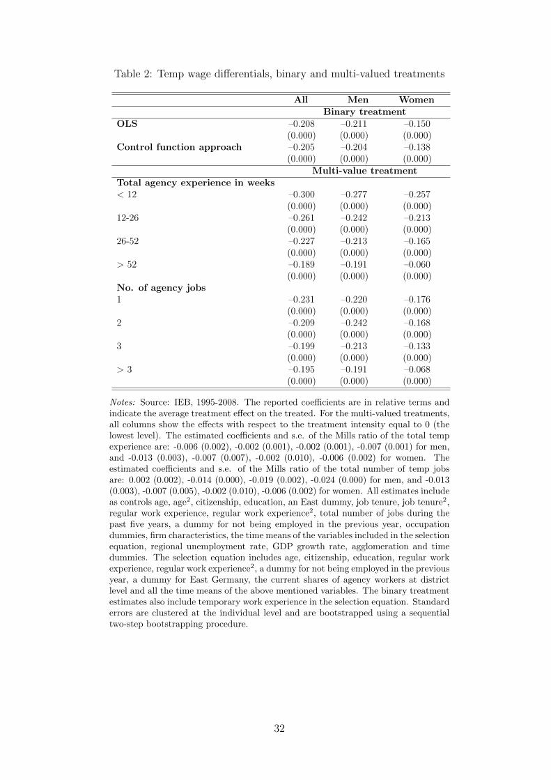
Table 2: Temp wage differentials, binary and multi-valued treatments

All Men WomenBinary treatment

OLS –0.208 –0.211 –0.150(0.000) (0.000) (0.000)

Control function approach –0.205 –0.204 –0.138(0.000) (0.000) (0.000)

Multi-value treatmentTotal agency experience in weeks< 12 –0.300 –0.277 –0.257

(0.000) (0.000) (0.000)12-26 –0.261 –0.242 –0.213

(0.000) (0.000) (0.000)26-52 –0.227 –0.213 –0.165

(0.000) (0.000) (0.000)> 52 –0.189 –0.191 –0.060

(0.000) (0.000) (0.000)No. of agency jobs1 –0.231 –0.220 –0.176

(0.000) (0.000) (0.000)2 –0.209 –0.242 –0.168

(0.000) (0.000) (0.000)3 –0.199 –0.213 –0.133

(0.000) (0.000) (0.000)> 3 –0.195 –0.191 –0.068

(0.000) (0.000) (0.000)

Notes: Source: IEB, 1995-2008. The reported coefficients are in relative terms andindicate the average treatment effect on the treated. For the multi-valued treatments,all columns show the effects with respect to the treatment intensity equal to 0 (thelowest level). The estimated coefficients and s.e. of the Mills ratio of the total tempexperience are: -0.006 (0.002), -0.002 (0.001), -0.002 (0.001), -0.007 (0.001) for men,and -0.013 (0.003), -0.007 (0.007), -0.002 (0.010), -0.006 (0.002) for women. Theestimated coefficients and s.e. of the Mills ratio of the total number of temp jobsare: 0.002 (0.002), -0.014 (0.000), -0.019 (0.002), -0.024 (0.000) for men, and -0.013(0.003), -0.007 (0.005), -0.002 (0.010), -0.006 (0.002) for women. All estimates includeas controls age, age2, citizenship, education, an East dummy, job tenure, job tenure2,regular work experience, regular work experience2, total number of jobs during thepast five years, a dummy for not being employed in the previous year, occupationdummies, firm characteristics, the time means of the variables included in the selectionequation, regional unemployment rate, GDP growth rate, agglomeration and timedummies. The selection equation includes age, citizenship, education, regular workexperience, regular work experience2, a dummy for not being employed in the previousyear, a dummy for East Germany, the current shares of agency workers at districtlevel and all the time means of the above mentioned variables. The binary treatmentestimates also include temporary work experience in the selection equation. Standarderrors are clustered at the individual level and are bootstrapped using a sequentialtwo-step bootstrapping procedure.

32

Table 3: Wage equations by treatment status, binary treatment

Men WomenAgency Regular Agency Regular

Foreign 0.013 –0.061 –0.020 –0.029(0.000) (0.001) (0.003) (0.001)

Age 0.025 0.044 0.054 0.069(0.001) (0.001) (0.001) (0.000)

Age squared/1000 –0.320 –0.384 –0.509 –0.524(0.000) (0.009) (0.020) (0.002)

Secondary degree with vt 0.002 0.037 –0.012 0.009(0.004) (0.002) (0.004) (0.002)

High school degree no vt –0.008 –0.101 –0.050 –0.114(0.030) (0.015) (0.004) (0.011)

High school degree with vt 0.005 0.030 –0.026 0.023(0.009) (0.000) (0.003) (0.001)

Polytechnics 0.026 0.067 –0.012 0.019(0.020) (0.007) (0.001) (0.008)

University degree 0.082 0.111 0.063 0.083(0.018) (0.002) (0.004) (0.002)

East –0.109 –0.102 –0.130 –0.080(0.000) (0.002) (0.004) (0.003)

Number of regular jobs (past 5 years) –0.005 –0.003 –0.003 –0.003(0.000) (0.000) (0.000) (0.000)

Work experience 0.001 0.051 0.029 0.065(0.000) (0.001) (0.002) (0.002)

Work experience squared/1000 – 3.657 5.776 –2.908 –7.366(0.190) (0.134) (0.197) (0.285)

Previously unemployed –0.052 –0.012 –0.067 0.019(0.002) (0.001) (0.002) (0.011)

Mills ratio –0.008 –0.000 –0.006 –0.012(0.002) (0.000) (0.000) (0.001)

N 495,289 2,927,145 163,793 1,489,384

Notes: Source: IEB, 1995-2008. The dependent variable in all estimations is thelog gross daily wage. All wage regressions also include as controls job tenure, jobtenure2, occupation dummies, firm characteristics, the time means of the variablesincluded in the selection equation, regional unemployment rate, GDP growth rate,agglomeration and time dummies. The selection equation includes age, citizenship,education, regular work experience, regular work experience2, a dummy for not beingemployed in the previous year, a dummy for East Germany, the current shares ofagency workers at district level and all the time means of the mentioned variables.Standard errors are clustered at the individual level and are bootstrapped using asequential two-step bootstrapping procedure.

33

Table 4: Post-temp earnings

Total agency experience in weeks No. of agency jobs< 12 12-26 26-52 > 52 1 2 3 > 3

All1 quarter –0.109 –0.076 –0.055 –0.053 –0.052 –0.081 –0.074 –0.087

(0.008) (0.006) (0.006) (0.028) (0.005) (0.008) (0.010) (0.011)2 quarters –0.106 –0.067 –0.015 –0.019 –0.023 –0.023 –0.046 –0.047

(0.007) (0.006) (0.006) (0.028) (0.004) (0.006) (0.010) (0.011)4 quarters –0.074 –0.020 –0.008 0.039 0.004 0.021 –0.017 –0.057

(0.009) (0.006) (0.006) (0.006) (0.004) (0.007) (0.010) (0.012)8 quarters –0.053 –0.011 0.029 0.070 0.026 0.036 0.030 –0.028

(0.010) (0.007) (0.007) (0.007) (0.005) (0.008) (0.013) (0.017)Men1 quarter –0.092 –0.055 –0.027 –0.030 –0.025 –0.041 –0.042 –0.049

(0.008) (0.006) (0.007) (0.026) (0.005) (0.007) (0.010) (0.011)2 quarters –0.079 –0.048 –0.014 –0.009 –0.006 –0.022 –0.041 –0.047

(0.008) (0.006) (0.006) (0.008) (0.005) (0.007) (0.010) (0.012)4 quarters –0.059 –0.033 –0.005 0.024 0.010 0.002 –0.016 –0.057

(0.009) (0.007) (0.007) (0.007) (0.005) (0.007) (0.011) (0.013)8 quarters –0.053 –0.028 –0.005 0.041 0.001 0.002 –0.027 –0.004

(0.011) (0.008) (0.008) (0.007) (0.005) (0.009) (0.014) (0.019)Women1 quarter –0.164 –0.084 –0.093 –0.090 –0.085 –0.087 –0.129 –0.139

(0.016) (0.012) (0.013) (0.016) (0.009) (0.015) (0.024) (0.031)2 quarters –0.121 –0.051 –0.044 –0.033 –0.046 –0.042 –0.059 –0.077

(0.016) (0.012) (0.012) (0.016) (0.008) (0.014) (0.024) (0.032)4 quarters –0.094 –0.012 0.030 0.103 0.038 0.050 0.027 –0.009

(0.019) (0.013) (0.013) (0.013) (0.009) (0.015) (0.026) (0.036)8 quarters 0.003 0.047 0.102 0.166 0.096 0.062 0.076 0.106

(0.022) (0.015) (0.014) (0.014) (0.009) (0.017) (0.031) (0.043)

Notes: Source: IEB, 1995-2008. The propensity score is estimated using a probitof treatment status on age, age2, citizenship, education, a dummy for not beingemployed in the previous year, a dummy for East Germany, job tenure, job tenure2,regular work experience, regular work experience2,total number of jobs during thepast five years, occupation dummies, firm characteristics, regional unemploymentrate, GDP growth rate, agglomeration, and time dummies. Caliper, δ = 0.0001.

34

App

endix

A(n

ot

for

publica

tion)

Tab

leA

-1:

Sel

ecte

dsa

mple

stat

isti

cs

All

Men

Wom

en

Tem

pN

on-t

emp

Tem

pN

on-t

emp

Tem

pN

on-t

emp

mea

nsd

mea

nsd

mea

nsd

mea

nsd

mea

nsd

mea

nsd

Ave

rage

real

gros

sw

age

52.8

0028

.900

89.9

0045

.600

52.8

0027

.700

96.0

0047

.200

53.0

0032

.300

78.1

0039

.500

Age

35.7

0010

.700

39.0

0010

.200

35.9

0010

.800

39.2

0010

.000

35.3

0010

.400

38.6

0010

.500

For

eign

0.21

60.

411

0.12

00.

325

0.22

70.

419

0.13

20.

339

0.18

20.

386

0.09

50.

293

Eas

t0.

203

0.40

20.

191

0.39

30.

211

0.40

80.

176

0.38

10.

181

0.38

50.

220

0.41

4E

du

cati

onS

econ

dary

degr

een

ovt

0.17

00.

376

0.08

90.

285

0.16

90.

374

0.08

90.

285

0.17

60.

381

0.09

00.

287

Sec

onda

ryde

gree

wit

hvt

0.68

80.

463

0.70

20.

458

0.71

70.

451

0.71

70.

450

0.60

30.

489

0.67

10.

470

Hig

hsc

hool

degr

een

ovt

0.00

80.

091

0.00

70.

086

0.00

70.

084

0.00

70.

082

0.01

20.

110

0.00

90.

093

Hig

hsc

hool

degr

eew

ith

vt0.

071

0.25

70.

081

0.27

30.

055

0.22

70.

064

0.24

50.

120

0.32

60.

115

0.31

9P

olit

echn

ics

0.02

90.

168

0.04

60.

209

0.02

50.

157

0.04

70.

211

0.04

00.

197

0.04

30.

203

Un

iver

sity

0.03

30.

178

0.07

50.

263

0.02

80.

164

0.07

60.

265

0.04

90.

215

0.07

20.

259

Pre

vio

us

emp

loym

ent

his

tory

Pre

viou

sye

arn

on-e

mpl

oyed

0.54

60.

498

0.17

30.

379

0.55

00.

498

0.18

00.

385

0.53

70.

499

0.16

00.

366

Job

ten

ure

(cu

rren

tjo

b)59

.200

69.5

0014

9.00

010

1.00

060

.800

70.8

0014

9.00

010

1.00

054

.400

65.1

0014

9.00

010

0.00

0N

o.ag

ency

jobs

(5ye

ars)

1.93

01.

460

0.22

10.

673

2.00

01.

530

0.25

00.

729

1.72

01.

210

0.16

60.

541

No.

all

jobs

(5ye

ars)

3.93

02.

540

2.49

02.

080

3.95

02.

580

2.53

02.

150

3.89

02.

420

2.41

01.

940

Wee

ksin

tem

pjo

bs(5

year

s)85

.900

79.8

006.

830

24.1

0089

.200

81.0

007.

690

25.9

0075

.800

75.1

005.

140

20.2

00W

eeks

inn

on-t

emp

jobs

(5ye

ars)

82.7

0074

.300

219.

000

64.1

0078

.700

72.9

0021

8.00

064

.900

94.7

0077

.200

220.

000

62.3

00O

ccu

pat

ion

Tec

hnic

aloc

cupa

tion

0.03

20.

176

0.07

80.

269

0.03

60.

186

0.10

00.

301

0.02

10.

142

0.03

50.

184

Man

ufa

ctu

rin

got

her

0.07

40.

262

0.16

60.

372

0.08

70.

281

0.20

60.

404

0.03

60.

186

0.08

60.

281

Man

ufa

ctu

rin

gm

etal

indu

stry

0.26

70.

442

0.17

80.

382

0.34

50.

475

0.24

50.

430

0.03

10.

173

0.04

50.

207

Lab

oure

r0.

318

0.46

60.

022

0.14

60.

319

0.46

60.

026

0.15

80.

318

0.46

60.

014

0.11

8C

leri

cal

occu

pati

on0.

148

0.35

50.

352

0.47

80.

139

0.34

60.

296

0.45

70.

178

0.38

20.

462

0.49

9S

ervi

ceoc

cupa

tion

0.16

00.

367

0.20

50.

403

0.07

50.

264

0.12

70.

333

0.41

70.

493

0.35

80.

479

Un

emp

loym

ent

rate

(dis

tric

tle

vel)

11.5

004.

650

11.0

004.

980

11.6

004.

700

10.8

004.

900

11.0

004.

470

11.3

005.

110

Sh

are

ofte

mp

s(d

istr

ict

leve

l)2.

220

1.39

01.

360

1.09

02.

210

1.38

01.

350

1.08

02.

240

1.41

01.

380

1.09

0

Ob

serv

atio

ns

659,

082

4,41

6,52

949

5,28

92,

927,

145

163,

793

1,48

9,38

4

35

Table A-2: Covariate balancing indicators before and after matching

N1 Median Bias Median Bias N1 off support N1 Median Bias Median Bias N1 off supportTotal agency experience After Before After No. of agency jobs After Before After

1 QuarterMen< 12 6,345 11.11 1.93 168 1 24,239 8.87 1.90 4,41412-26 11,820 9.41 2.15 510 2 9,360 11.02 1.34 3,43226-52 13,205 10.40 2.24 1,700 3 4,410 12.98 2.28 1,655> 52 13,367 12.50 5.66 8,597 > 3 3,704 15.77 5.17 2,018N0 2,019,616 N0 2,019,616

Women< 12 2,444 11.98 3.33 39 1 9,769 13.66 3.58 2,17612-26 4,501 12.55 3.49 223 2 3,180 15.49 3.07 1,05126-52 4,393 15.42 3.54 625 3 1,140 14.34 2.88 507> 52 3,040 16.69 2.18 3,710 > 3 707 18.38 4.95 445N0 1,149,028 N0 1,149,028

2 QuartersMen< 12 5,287 9.78 1.27 44 1 22,457 7.93 2.25 2,75212-26 9,825 9.00 1.46 200 2 8,707 10.96 3.22 2,38426-52 9,886 10.34 2.84 1,421 3 3,664 11.54 3.66 1,212> 52 9,782 11.79 1.41 8,920 > 3 2,827 14.51 6.37 1,362N0 1,780,655 N0 1,780,655

Women< 12 2,089 11.79 1.51 11 1 9,201 13.98 3.17 1,47512-26 4,126 13.39 2.28 53 2 2,899 15.34 3.53 75226-52 3,744 15.83 4.01 651 3 970 17.30 2.05 410> 52 2,724 16.18 2.11 3,206 > 3 594 18.37 4.61 303N0 1,011,421 N0 1,011,421

4 QuartersMen< 12 4,021 11.26 1.84 31 1 4,021 11.26 1.84 3112-26 7,488 9.38 3.01 193 2 7,488 9.38 3.01 19326-52 7,866 7.95 3.03 639 3 7,866 7.95 3.03 639> 52 10,698 10.34 2.10 3,374 > 3 10,698 10.34 2.1 3374N0 1,544,083 N0 1,544,083

Women< 12 1,,613 11.23 2.98 3 1 8,049 15.78 4.25 56812-26 3,196 15.12 4.25 95 2 2,525 15.89 4.05 29226-52 3,178 15.97 4.40 303 3 801 18.92 3.37 165> 52 3,414 17.6 2.73 1,137 > 3 445 18.44 4.96 94N0 875,087 N0 875,087

8 QuartersMen< 12 2,551 13.06 1.57 16 1 13,231 8.44 1.25 25912-26 4,679 10.11 1.53 46 2 4,512 11.73 1.71 15926-52 5,123 8.81 1.59 105 3 1,490 12.28 1.79 65> 52 7,537 11.21 1.89 606 > 3 867 16.93 3.20 80N0 1,314,057 N0 1,314,057

Women< 12 1,011 11.83 2.17 2 1 5,675 16.43 1.43 6812-26 2,016 14.88 2.36 17 2 1,627 17.84 2.23 4426-52 2,244 18.57 1.51 27 3 485 19.51 2.81 18> 52 2,588 18.44 2.41 148 > 3 213 15.91 3.25 13N0 709,127 N0 709,127

Notes: Source: IEB, 1995-2008. N1 indicates treated sample and N0 the control sample. N1 off support indicates the number ofobservations not in the common support. Median absolute standardised bias before and after matching, with median taken over all the 52regressors. Following Rosenbaum and Rubin (1985), for a given covariate X, the standardised difference before matching is the differenceof the sample means in the full treated and non-treated subsamples as a percentage of the square root of the average of the samplevariances in the full treated and non-treated groups. The standardised difference after matching is the difference of the sample means inthe matched treated (i.e. falling within the common support) and matched non-treated subsamples as a percentage of the square root

of the average of the sample variances in the full treated and non-treated groups. Hence Bbefore(X) = 100X1−X0√

(V (X1)−V (X2))/2and

Bafter(X) = 100X1−X0√

(V (X1)−V (X2))/2

.

36