Does Relationship Specific Investment Depend

on Asset Ownership? Evidence from a Natural

Experiment in the Housing Market

Georg GebhardtUniversity of Munich∗

May 2010

Abstract

In this paper, I test the most basic prediction of Grossman and Hart

(1986): Allocations of asset ownership that expose a party to ex-post ex-

propriation reduce this party’s ex-ante relationship specific investments. In

the empirical context of the German housing market, I find that relationship

specific investments, such as bathroom renovations, are more frequent if the

occupant is protected against expropriation because he owns his home. To

avoid the endogeneity of the homeownership allocation, I rely on the natu-

ral experiment of the German reunification: Under the communist regime,

ownership existed but was economically meaningless; yet after reunifica-

tion, ownership unexpectedly reacquired legal force.

Keywords: Relationship Specific Investment, Hold-Up, Natural Experi-

ment

JEL-Classification: D23, D86, C23

∗Department of Economics, University of Munich, Ludwigstr.28 (Rgb.), D-80539 Munich,Tel.: +49 89 2180 2876, e-mail: Georg.Gebhardt@LRZ.uni-muenchen.de. I would like to thankKlaus Schmidt, Tomaso Duso, Florian Englmaier, Nicola Fuchs-Schündeln, Roland Ismer, NicoKlein, Tymofyi Mylovanov, Arno Schmöller, Matthias Schündeln, Ferdinand von Siemens, Kon-rad Stahl, Christina Strassmair, Daniel Sturm, and Jean Tirole. Financial support by DeutscheForschungsgemeinschaft through grant SFB TR 15 is gratefully acknowledged.

1

1 Introduction

If the parties to a contract have to make relationship specific investments, they

face a hold-up problem (Williamson 1975) that induces them to underinvest. In a

classic paper, Grossman and Hart (1986) argue that the parties can mitigate this

problem through the allocation of ownership rights. Ownership of an asset im-

proves investment incentives because it improves the bargaining position of the

investor when he negotiates his share of the surplus from theinvestment. A large

theoretical literature explores the implications of this argument, but it is difficult

to empirically test its most basic prediction that asset ownership affects invest-

ment decisions. The reason is an endogeneity problem: The hold-up model not

only predicts asset ownership to determine investment, butalso investment oppor-

tunities to determine asset ownership, as the parties allocate assets to mitigate un-

derinvestment. In this paper, I address this problem by using the exogenous vari-

ation of homeownership that resulted from the abrupt fall ofcommunism in East

Germany and the subsequent reunification with West Germany.Under commu-

nism, private ownership of property existed but was devoid of economic content;

after reunification, however, homeownership unexpectedlyre-acquired its full le-

gal force. I show that households who became homeowners during communism

undertake more relationship specific investments, such as bathroom renovations,

than households who became tenants.

I apply the argument of Grossman and Hart (1986) to the context of the hous-

ing market. The model predicts underinvestment in dwellingspecific fixtures

(bathrooms, kitchens) in rental housing but not in owner occupied housing.1 Of-

ten landlords let houses largely unfurnished, as they anticipate that tenants will

overuse leased furniture. But there should be no inefficiency as tenants can buy

their own furniture. Similarly landlords let houses with a varying degree of kitchen,

bathroom, and other fixtures. As in the case of furniture, landlords should be ex-

1Why there is rental housing even though it induces underinvestment is beyond the scope of thispaper; most likely, the allocation of ownership serves morethan one role in the housing markets;e.g., financial market imperfections may require that ownership sometimes rests with the landlord.

2

pected to underinvest as they anticipate a moral hazard problem. But, unlike in

the case of furniture, tenants may not make up for the lack of investment by the

landlord because they fear that the landlord will expropriate them. Under Ger-

man tenancy law, the tenant is protected against expropriation by rent control and

eviction protection laws as long as he stays in the dwelling;if he has to move

out, however, the tenant is not entitled to compensation. Typically the landlord

chooses the new tenant, who then negotiates with the old tenant to buy the in-

vestment. Because the old tenant has a low threat point (removing the investment

and selling it separately), he will receive only a share of the surplus. Anticipating

this outcome, he should underinvest.2 In contrast, an owner occupier is protected

by his asset ownership; he can always sell or rent the apartment on a competitive

market.

To establish empirically that owner occupancy causes an increase in the reno-

vation frequency, I instrument homeownership in later years by home ownership

immediately after the reunification of the East German “German Democratic Re-

public” (GDR) and the West German “Federal Republic of Germany” (FRG). The

instrument induces an exogenous variation of the ownershipstructure because the

East German state diluted ownership rights to a degree that homeownership was

acquired quasi randomly as a by-product of dwelling choice.Only after the Ger-

man reunification, the full range of ownership rights of the West German legal

system was suddenly and unexpectedly awarded to East Germanhomeowners.

Using the natural experiment of the German reunification is by now a well estab-

lished practice in economics; see e.g., Fuchs-Schündeln and Schündeln (2005),

Alesina and Fuchs-Schündeln (2007) or Redding and Sturm (2008).

Using data on home renovations in East Germany for the years 1997–2002

from the German Socioeconomic Panel (GSOEP), a rich household panel data

set, I find an effect of ownership on investment that is both statistically significant

2It is in the interest of the landlord to first choose a new tenant, who then negotiates with theold tenant. In this way, the new tenant can acquire the fixtures at a lower price. Because the newtenant anticipates this outcome, he has a higher willingness to pay for the dwelling. The landlordcan extract this willingness to pay by relying on competition between potential new tenants.

3

and large. The yearly renovation probability for bathroomsdrops by approxi-

mately 6 percentage points if a household rents, controlling for many household

and building characteristics. I add controls for potentialalternative effects of GDR

homeownership on the investment probability, such as the fact that owners are

wealthier or anticipate to stay longer in their home. The introduction of these

controls has little effect on the size or statistical significance of the coefficient of

ownership. I apply three robustness checks: (1) I use as dependent variables TV-

set and car purchases; i.e., not dwelling specific investments, on which ownership

should not have a positive effect. This is exactly what I find in the data. (2) I

confirm that a comparable relationship between ownership and investment exists

in the West German housing market. (3) I replicate the analysis for the early years

after the reunification (1992–1996) and get almost exactly the same coefficient on

ownership.

There is a small but growing literature that tests comparative static predic-

tions of applied hold-up models for contract and organizational forms in different

industries. These papers, by and large, confirm the predictions in several indus-

tries such as trucking (Baker and Hubbard 2003, Baker and Hubbard 2004), de-

fense (Crocker and Reynolds 1993), footwear (Woodruff 2002), and biotechnol-

ogy (Lerner and Malmendier 2005). A related literature (Besley 1995, Jacoby and

Mansuri 2008) studies the role of property rights in developing countries. Most

closely related is Field (2005, 2007) who studies the impactof property rights

on investment in urban housing. In contrast to these papers,I focus on a large

and mature market in an industrialized country and I do not study contracts or

organizational forms but directly the impact of asset ownership on investment.

4

2 A Theoretical Framework

2.1 The German Housing Market

In Germany landlords and tenants are bound by rent control and eviction protec-

tion laws. In a new lease as well as in an ongoing tenancy, tenants and land-

lords can set the rent essentially at any level by mutual agreement. Unilaterally,

however, the landlord can adjust the rent only within very tight limits. She is con-

strained, according to Section 558 of the German Civil Code (Lützenkirchen 2003,

pp. 540–594), by the average rent paid for comparable dwellings; moreover, she

must not increase the rent by more than 20 percent within three years (Lützen-

kirchen 2003, p. 543). If the landlord upgrades the dwelling, she can charge a

markup over the comparison rent according to Section 559 of the German Civil

Code (Lützenkirchen 2003, pp. 594–620). Unless the tenant is in breach of con-

tract, it is nearly impossible for the landlord to unilaterally terminate the lease

(Lützenkirchen 2003, pp. 1281–1383). The landlord may evict the tenant if she

moves in herself, but such owner move-ins are difficult in practice.

The legal default leaves investments by tenants largely unregulated. To invest,

the tenant must obtain the permission of the landlord, but the tenant owns the

investment and can decide to remove it. The landlord can try to expropriate the

tenant by raising the rent, but typically she cannot do so as long as the tenant

stays in the dwelling due to rent control and eviction protection. If the tenant

moves out, however, he is not entitled to a compensation under the legal default

(Lützenkirchen 2003, pp. 964–968).

The tenant and the landlord can conclude a standard contractthat protects the

tenant against expropriation. In such a contract, called modernization agreement

(Lützenkirchen 2003, pp. 968–973), the tenant agrees to undertake a specific in-

vestment, and the landlord gives her permission. The landlord can forego, for a

fixed period of time, the right to rent increases according toSections 558 and 559

of the German Civil Code and the right to terminate the lease.In particular, she

can give up the right to move into the dwelling herself. The landlord can commit

5

to pay a redemption sum to the tenant if the latter moves out. Usually this sum de-

clines over time, but there is no mechanism to condition the transfer on the actual

value of the investment at the time of the move.

To analyze the investment incentives in the housing market,I develop a model

that reflects the stylized facts of German tenancy law. I assume that the landlord

fails to make at least some investments that an owner occupier would make, e.g.,

because she anticipates moral hazard problems. I only modelthe additional in-

vestments by the occupant, comparing owner occupiers with tenants. Assuming

that the landlord underinvests seems plausible; still, I will test this assumption as

part of a joint null hypothesis in the empirical part. The null hypothesis will be

that investment in rented and owner occupied dwellings is the same. This hypoth-

esis includes the case that landlords have the same investment incentives as owner

occupiers to begin with. The only contract I consider in my model is the standard

modernization agreement. This restriction can be justifiedbecause the modern-

ization agreement is the only contract found in standard legal texts; however, this

assumption, too, will be tested as part of the null hypothesis. If there are other

contracts, unknown to me, that solve the hold-up problem, investment will be the

same in owner occupied and rental housing. In this case I willnot be able to reject

the null hypothesis that asset ownership does not matter forinvestment.

2.2 Setup

An occupant of a dwelling, which either he or a landlord owns,has to decide on an

investment that is specific to the dwelling; e.g, a new kitchen or bathroom. With

some probability, the occupant has to move out of his home before he can enjoy

the investment. In this case a new occupant moves in, and the original occupant

must decide whether to leave the investment in the dwelling or not.

The exact timing is as follows: At time 1, the original occupant must decide

whether to invest or not.3 His investment decision is expressed by the indicator

3In the case of a rental unit, legally the landlord has to consent. But without additional ex-ante contracting that increases consensually the rent, shecannot hold-up the tenant by denying

6

variableI ∈ {0,1}, whereI equals 1 if the original occupant invests. In this case

he incurs an investment cost ofK. At time 2, a state of the worldθ ∈ {θS,θM}

is realized, which indicates whether the occupant stays (θS) or moves out of the

dwelling (θM). The probability that the original occupant moves out is denoted by

q. In stateθM, the original occupant can remove the investment (if there is one).

His removal decision is expressed by the indicator variableR∈ {0,1}, whereR

equals 1 if the occupant removes the investment.

All agents are risk neutral, have quasi linear (in money) utility functions, and

do not discount. If the original occupant has invested and stays (θ = θS), he

enjoys a utility ofxS from the investment. The utility from no investment is 0. If

the original occupant moves out (θ = θM), he can remove the investment and take

it with him, which gives him a utility ofxM; in the case of a bathroom or kitchen

xM is likely to be small and may be zero. Alternatively, the original occupant can

leave the investment in the dwelling; in this case there is a competitive rental or

housing market market, on which potential new occupants arewilling to payy for

the investment. Asy> xM, efficiency requires that the original occupant leave the

investment in the dwelling.

2.3 Results

Owner Occupancy vs. Tenancy

In this section, I compare the investment incentives of an owner occupier with

those of a tenant. An owner occupier can always extract all the surplus generated

by the investment. Thus, he takes the investment and removaldecisionIO andRO

permission because she cannot extract payments. The landlord may, on the other hand, profit fromthe investment if the tenant has to move out; therefore, the landlord would always consent, and Imodel investment directly as the tenant’s choice.

7

given by

IO(q,xS,y) =

{

1 if K ≤ (1−q)xS+qy;0 if K > (1−q)xS+qy; and

RO = 0.

If the original occupant is a tenant and the dwelling is ownedby a landlord, the

occupant’s investment incentives are different. Suppose that the landlord cannot

extract a share of the surplus generated by the investment aslong as the tenant

stays in the dwelling;4 then the tenant enjoys a utility ofxS from the investment

in stateθS. If he moves out, he can get a utility ofxM if he takes the investment

with him, while the landlord could gety if the investment remains in the dwelling.

To induce the tenant not to remove the investment, the landlord can offer him a

transferT. I assume that the landlord and the tenant negotiateT at time 2, after

they have learnedθ , but before the tenant decides on removal. To model the

negotiation process, I use a Nash bargaining solution in which each party gets

half of the surplus.5

If the tenant stays, he keeps the whole return on his investment. If the tenant

has to move, he prefers to take the investment with him unlessthe landlord com-

pensates him. Because this decision is inefficient, the tenant negotiates a transfer

with the landlord and leaves the investment in the dwelling.According to my

assumption on the bargaining outcome, the transfer equals the tenant’s outside

option plus half of the surplus; i.e.,

T =y+xM

2.

4This assumption reflects that the tenant is protected by rentcontrol and eviction protectionlaws so that the landlord can neither raise the rent unilaterally nor force the tenant to accept ahigher rent by threat of eviction. The main result of this section, that the tenant underinvests, holdsa fortiori if the landlord extracts a share of the surplus while the tenant stays in the dwelling.

5For simplicity, I assume that the tenant negotiates with thelandlord, who then sells the in-vestment under competition to the new occupant. In reality,the old occupant is more likely tonegotiate directly with the new occupant, while the landlord extracts the surplus beforehand. Theresulting payment streams are identical.

8

Because he does not get the whole surplus in stateθM, the tenant sometimes does

not invest even though an owner occupier would invest in the same situation; i.e.,

the tenant takes the following investment and removal decisionsIT andRT :

IT(q,xS,y) =

{

1 if K ≤ (1−q)xS+qy+xM2 ;

0 if K > (1−q)xS+qy+xM2 ;

and

RT = 0.

I obtain the following proposition:

Proposition 1 (Owner occupancy vs tenancy)If

(1−q)xS+qy+xM

2< K < (1−q)xS+qy,

the investment does not pay off for a tenant, but it is profitable for an owner

occupier. For any other value of K, a tenant takes the same investment decision

as an owner occupier.

The Modernization Agreement

So far, I have assumed that the parties cannot write an ex-ante contract to mitigate

the hold up problem. There is, however, a standard ex-ante contract in German

tenancy law, the modernization agreement. In a short theoretical analysis, I high-

light what could be the main drawback of this contract.

In contrast to the last section, the landlord now can make a contract offer to the

tenant at time 0 before the tenant can invest. In line with thestylized facts of the

modernization agreement, the landlord can commit himself to pay a compensation

for any investment if the tenant moves out.6 Furthermore, the parties can contract

any ex-ante transfer; this assumption reflects the fact thatthe parties can always

set the rent consensually at any level.

6The landlord may also contractually forego any remaining right to unilateral rent increases ortermination by notice. But for my analysis these options do not matter, as I anyway abstract frompotential expropriation while the tenant stays.

9

Referring toy as the market value of the investment, I get the following result:

Proposition 2 (Modernization agreement) Suppose the parties can ex-ante con-

dition the transfer upon the market value of the investment.Then there exists a

modernization agreement that replicates the investment incentives of an owner

occupier.

If the parties can tie the compensation to the ex-post marketvalue of the in-

vestment, they can solve the hold-up problem. The landlord offers the tenant a

modernization agreement that allows the tenant to decide whether to invest and

stipulates that the landlord must redeem the investment according to its market

value. Such a contract replicates an owner’s payment streamand implements an

owner’s investment and removal decisions.7

Thus, there is a simple solution to the hold-up problem if thecontract can

condition on the market value of the investment. Yet the standard modernization

agreement does not seem to provide a mechanism to do so. If landlords and tenants

do not use more comprehensive contracts, even though there is underinvestment,

it must be because it is difficult to contract on the market value of an investment.

As the market value of investment is an observable variable,the contracting par-

ties seem to face an instance of the of the observable-but-unverifiable-information

problem.

In the next section, I study empirically how the investment probability depends

on ownership allocation. I compare the yearly investment probability in owner

occupied houses and in rental houses. The null hypothesis isthat landlords and

tenants manage to solve the hold-up problem by means of formal or informal

contracting; hence asset ownership does not play a role in protecting investment

incentives and there is no difference in investment probabilities between rental

and owner occupied housing.8 The alternative hypothesis is that the landlords and

7This result is robust to an uncertainy or anxS that is private information of the old occupant.Even if removal was efficient in some states of the world, or the moving choice was endogenous,the tenant would always choose efficiently given the suggested contract.

8The null also includes the hypothesis that there is no contracting problem in the first place,e.g., because landlords have enough incentives to renovate.

10

tenants fail to solve the hold-up problem by formal or informal contracts so that

they have to rely on asset ownership to protect investment incentives. In this case I

should observe an investment probability that is higher in owner occupied housing

than in rental housing.

3 Institutional Setting and Data

In this section, I present the data that I use to investigate whether homeownership

increases the probability of relationship specific investments or not. To establish a

causal relationship, I must deal with the potential endogeneity of homeownership.

An unobservable omitted variable could drive a positive correlation of investment

probability and homeownership; e.g., many households thathave secure and stable

employment prospects in one place may find it worthwhile and can afford to incur

the fixed costs associated with buying a house. For the same reason, they may be

able and willing to customize their home by investing in renovations. Even if there

is a contracting problem, the coefficient in a regression analysis could exaggerate

its size due to reverse causality; e.g., if households anticipate the contracting prob-

lems in rental housing, households with a preference for frequent renovations will

be more inclined to buy.

To obtain an exogenous variation of homeownership, I use thehomeownership

allocation in East Germany immediately after the fall of thewall as an instrument

for the homeownership allocation in later years. To justifymy choice of instru-

ment, I present an outline of the legal situation and the historic development of

the housing market in the GDR.

3.1 Housing in the GDR

Tenancy and Real Estate Law in the GDR

For the whole of its existence, the communist regime of the GDR pursued the goal

of abolishing private property. In the 1970s the GDR implemented property leg-

11

islation that abolished private ownership of investment goods but allowed private

ownership of consumption goods, including owner occupied housing (Bundes-

ministerium für innerdeutsche Beziehungen 2000, entry “Eigentum”). Privately

owned rental housing continued to exist in a legal grey area:Regulations diluted

the property rights of landlords to a degree that ownership became meaningless for

all practical purposes, while it raised the rights of tenants to a level that equalled

those of owner occupants.

Once an East German had signed a lease, he was almost completely protected

against interference by the landlord. The landlord needed acourt order to evict

a tenant, which was near to impossible to obtain (Buck 2004, p. 363). De jure,

the state could evict owners and tenants alike if they occupied too much space

(Hoffmann 1972, p. 323). De facto, in the 1980s tenants oftenpaid rents for

apartments but left them empty to retain control over them for future use; they did

so without consequences (Herbst, Ranke, and Winkler 1994, entry “Wohnraum-

lenkung”).

East Germans could conclude a (standardized) rental contract only if they had

a permit from the government (Buck 2004, p. 363). If an East German bought a

vacated dwelling or if her tenant moved out, she still neededa government permit

to move in (Hoffmann 1972, p. 319). To build a home, GDR citizens needed a

permit as well (Buck 2004, p. 160). Permits allocated East Germans to dwellings

because government regulation had dismantled the price mechanism in all but in

name. In all markets, East Germans faced prices that were setby the state; often

the state set prices too low to reflect scarcity. Rents and real estate prices were

frozen at the levels of the year 1936 (Häußermann, Glock, andKeller 2000, p.7).

Prices for new construction and building materials were regulated as well. The

state subsidized the construction of owner occupied homes by cheap credit and

tax reductions for those who managed to get a permit (Buck 2004, pp. 159–164).

At such low prices, East Germans demanded more housing than the communist

economy could deliver: In 1989, East Germans paid only 3 percent of their net

income for housing (Buck 2004, p. 372), but 778,352 households were waiting for

12

a unit (Buck 2004, p. 361).

Under the permit system households fared better if they conformed to explicit

and implicit, political and social criteria (Herbst, Ranke, and Winkler 1994, en-

try “Wohnraumlenkung”); e.g., the state used permits to reward citizens who were

loyal to the communist regime (Buck 2004, pp. 367–369). Suchhouseholds were

able to secure themselves systematically better housing than others. Whether

housing quality was correlated with ownership remains a priori unclear. East Ger-

mans prized suburban single family homes, which were often owner occupied, but

also newly built high rise apartments, which were always rented.

Most private landlords were unable to pay for renovations and let the houses

decay (Buck 2004, pp. 365–366) because they received only the government set

low rents. The state and cooperatives did hardly better because the communist

regime focused on industrial scale new construction and neglected reconstruction

(Buck 2004, p. 351).

Historic Development of Homeownership in the GDR

Private ownership of real estate continued to exist until reunification. Owners of

real estate, unlike entrepreneurs or farmers, were never expropriated. They always

owned whole buildings; i.e., either apartment buildings orsingle family homes.

Condominiums did not exist in Germany before World War II andthe GDR never

introduced them. The regime did not allow private owners theconstruction of new

rental buildings (Hoffmann 1972, p. 347). Private owners ofexisting apartment

buildings had no effective control over their property, received the low government

fixed rent payments, but had to maintain the buildings. As a consequence many

owners gave away their houses to the state (Buck 2004, p. 245), which introduced

permits to control the unwanted donations (Hoffmann 1972, p. 349 and pp. 352–

353).

In the immediate post-war period, East Germans were allowedto build owner

occupied single family homes; however, over time the state brought this construc-

tion to a virtual standstill (Buck 2004, p. 245). In a policy reversal starting from

13

the mid 1970s and lasting until reunification, the communistregime did not only

allow but even subsidized the private construction of owneroccupied homes if

it decided to grant a permission; however, the permissions were granted within

strict limits (Häußermann, Glock, and Keller 2000, p. 7, Buck 2004, p. 331).

The regime granted most permits on the countryside, where itcould not construct

housing on an industrial scale. With none of these initiatives, however, the com-

munist regime halted the increase of public ownership of thehousing stock in the

GDR.

Summary

For all practical matters, there was little difference between owning or renting a

house in the GDR. As the reunification and its implications for property rights

was unforeseen, East Germans are unlikely to have cared whether they owned or

rented. Given the notorious shortage of dwellings, few if any East Germans ever

had the choice between two equivalent houses, one of them forrent the other one

for sale. East Germans simply looked for the type of housing best suited to their

needs no matter if it was for rent or for sale. Thus, the homeownership allocation

in 1990 is independent of omitted variables that would simultaneously influence

investment behavior and homeownership in a market economy.

3.2 The German Socioeconomic Panel

The data come from the German Socioeconomic Panel (GSOEP).9 The SOEP is

a representative longitudinal study of private householdsin Germany. It started in

1984 in what was then the Federal Republic of Germany (FRG) and was extended

in 1990 (after the fall of the wall but before reunification) to the area of the former

German Democratic Republic (GDR). Each year the the fieldwork organization

TNS Infratest Sozialforschung returns to the same households. The sample is

very stable: Of the 2 179 households with 4 453 members that were randomly

9See Wagner, Frick, and Schupp (2007) for a description.

14

selected for the “SOEP East” sample in 1990, 1 592 householdswith 2 892 still

participated 18 years later.

In its questionnaire the survey records on household level whether there have

been certain renovations, e.g., of the bathroom or the kitchen, and whether the

household rents or owns. In addition the survey contains information on a number

of characteristics of the dwelling (e.g., condition, type,and building year) as well

as on the household (e.g., income). Some of these variables the survey records on

the person level. In this case I use the characteristics of the head of household as

a proxy for the characteristics of the whole household.

For my analysis I use information on different household related investments.

For my main results I use yearly data on bathroom renovations. The data is binary;

i.e., it indicates whether the household reports a bathroomrenovation in a partic-

ular year or not. It includes all renovations no matter whether owner, tenant, or

landlord paid for them. Furthermore I have information on renovations of kitchens

and data on household related investments that are not relationship specific to the

dwelling, such as TV-set or car purchases.

I use the years from 1997 until 2002 in my main analysis. Afterreunification

East German homeowners often faced restitution claims by former owners who

were forced to sell houses when they left the GDR. For the years before 1997

I cannot rule out that the ownership of a house was disputed. Still I report the

results for the years 1992–1996 in Section 4.4 as a robustness check; the results

are virtually identical. I need the data of the years from 2002 to 2007 to construct

a variable that indicates whether a particular household still lives in the same

dwelling after five years.

In 1990, 2179 Households formed the East German sample of theGSOEP.

They were interviewed beginning in June, 1990, one month before the currency

union and four months before the reunification with West Germany. Only a few

months earlier, on November 9, 1989, they had witnessed the fall of the wall

but they still lived in the German Democratic Republic, a state separate from the

Federal Republic of Germany. Of these households 626 or 28.8percent owned

15

the unit they lived in.

Comparing owners and tenants, I find no indication that either group on av-

erage was favoured by the communist regime. To determine thecloseness to the

regime, I consider whether the household had a telephone. The East German state

was unable to provide even a majority of households with phone connections.

Typically households favoured by the regime were more likely to obtain a phone.

In my data, I find that 22.5 percent of homeowners have a phone connection com-

pared to 21.5 percent of tenants.

Because I instrument homeownership in later years by homeownership in

1990, I can use only households that were in the East German sample in 1990.

(2179 households). I cannot include households that split from an existing house-

hold, e.g., because married couples divorce or children move out. Over the six

years from 1997–2002 I should obtain a maximum of 13074 observations, but

due to panel attrition and missing values I only have 8351 observations for which

I have information on ownership and bathroom renovations.

In the data I observe an increase in homeownership that reverses the depressed

homeownership levels in the GDR. In 1997, already 36 percentof East German

households owned their home, and until 2002 this percentagerises to almost 42

percent. On average around 40 percent of households in my sample own the unit

they live in.

For bathroom renovations, I observe a decrease over time in the data, which

suggests that initially East German households were still in the process of upgrad-

ing their homes to Western standards. In 1997, around 10 percent of households

renovated their bathrooms, equalling one renovation every10 years. In 2002, only

slightly more than 3 percent of households renovated their bathrooms, equalling

one renovation every 31 years. On average around 6 percent ofhouseholds in my

sample renovate their bathrooms in any given year (once every 17 years).

16

4 Evidence from Regressions

4.1 Impact of Homeownership on Bathroom Renovations

For my regression analysis, I pool data from the years 1997–2002. An observation

indexed byi is one household in one year. I compare households that own their

home (owni = 1) to households that do not (owni = 0) and consider the impact of

homeownership on bathroom renovations. The dependent variable is the binary

variablerenovi, which takes the value 1 if a particular household has reported

that its bathroom has been renovated in a particular year. The variable indicates

renovations by the tenant as well as the landlord or an owner occupier. I estimate

the following linear probability model with pooled OLS:10

renovi = α +βowni +Θ′yeari +Γ′BCi,B+Γ′

WCi,W +Γ′NCi,N + εi (1)

In all specifications, I include a vector of year dummies (yeari) and a vector of

baseline controlsCi,B including income. In four specifications, I instrument own-

ership in a particular year by ownership in 1990. In three of the instrumental

variable specifications, I control for wealth differencesCi,W. In one of these spec-

ifications, I add controls for other non-contracting effects of ownership in 1990

Ci,N. All standard errors are robust and clustered at the household level. See Table

A-1 in the appendix for summary statistics of all variables.

OLS Regression

I first implement an OLS regression of equation (1), including only baseline con-

trols Ci : dummies for new buildings (built after reunification), measures of the

refurbishment need of the house11 and the distance from the next city center (on a

10The results are essentially identical with the probit specification reported in the appendix. SeeTable A-2 for the regressions and Table A-3 for the marginal effects of ownership on bathroomrenovations.

11Refurbishment need contains the answer to the questionnaire question “What is the conditionof your house?” on a scale from 1 (“in good condition”) to 4 (“is ready for demolition”). I use the

17

scale from 1 to 6, 6 being the most distant), and household income (ΓW = ΓN = 0,

column (1) in Table 2).

I calculate household income to include income from labor, government trans-

fers (or taxes) and wealth, in particular an imputed rent forowner occupied hous-

ing. I use the yearly household income after taxes and government transfers pro-

vided by the survey and add to this income an imputed rental value if the house-

holds owns its home. The imputed rental values is provided inthe SOEP and

consists of a rent estimate minus operating costs. The rent estimates are derived

from the information on tenant households in the panel. I usethe consumer price

index provided by the SOEP to to calculate year 2000 Euros andadjust the income

for household size by dividing by the square root of the number of household

members.

In the first line of Table 1, I report summary statistics of themy income vari-

able for households that owned in 1990 and for those that rented. Households

that owned have an income that is approximately 2000 Euros higher per year.

This difference is almost entirely due to income from wealth, which I report in

the second line. Income from wealth contains interest, dividends, asset flows and

rental income and the imputed rental value. The difference in income from wealth

plausibly results from the high return real estate owners derived from their invest-

ment in the GDR compared to other investments. Households who managed to

buy or keep a house incidentally made the best investment choice possible, given

that the reunification occurred. East Germans had only low return financial in-

vestment opportunities and, in 1990, they could convert only a limited amount of

financial wealth into Deutsche Mark at a favorable exchange rate. If they invested

in durable consumption goods like cars, they almost completely lost their money

upon reunification when better products became available. But if they bought,

built, or did not sell a house at the artificially low prices inthe planned economy

of the GDR, they should have earned a considerable return on their investment.

value of the preceding year to avoid endogeneity. I have confirmed that the effect of this variableis almost perfectly linear so that I include the numerical value rather than three dummy variables.

18

Table 1: Descriptive Statistics Yearly Income and Wealth East German House-holds 1997–2002 (1000e).

Tenant 1990 Homewoner 1990Mean St. Dev. Mean St. Dev.

Income 16.1 6.8 18.2 7.0Income from wealth 0.7 1.7 2.7 3.0

Wealth 29.8 58.4 88.7 71.2

Notes: An observation is one household in one year for which data on bath renovations is non-missing. All values in year 2000 Euros.

With these baseline controls homeownership increases the probability of a

bathroom renovation in any given year by 5.7 percentage points. The standard

error is 0.007; I am able to reject the null hypothesis that homeownership does not

influence bathroom renovations at the 0.1 percent level. Thesize of the effect of

homeownership is economically relevant — it roughly equalsthe sample mean of

the renovation probability of 6 percent.

The sign and magnitude of the covariates in the regression seem sensible. A

new dwelling, built after reunification, decreases the renovation probability by 1.9

percentage points. A one unit increase in the refurbishmentneed increases the

renovation probability by 3 percentage points.12

Income has no significant effect on the renovation probability. As income

does, however, have a significant positive effect on the purchase of cars and TV-

sets (see Table 7) and, in most specifications, on kitchen renovations (see Table

5), the insignificance is unlikely to be due to measurement error, but rather reflects

the preferences of East Germans in those years: They prefer to spend additional

12One might be worried that refurbishment need is correlated with lagged bathroom renovations,which, in the presence of residual autocorrelation, could lead to biased estimates. To address thisconcern, I report in column (2) of Table A-4 in the appendix a specification that explicitly containslagged renovations. The coefficient on ownership is highly significant and almost the same sizeas in the baseline specification. This specification is estimated consistently if it is dynamicallycomplete (Wooldridge 2002, pp. 173–177). To verify that it is dynamically complete, I regresslagged residuals on residuals in column (3); the lagged residuals are not significant; there is noresidual autocorrelation.

19

income on goods such as cars, TV-sets and kitchens rather than new bathrooms.

Instrumental Variable Regression — Baseline

I instrument homeownership in the years from 1997 to 2002 by homeownership in

1990, i.e., before reunification. In Table 3, I report the results of the first stage re-

gression. These results indicate that homeownership in 1990 has strong predictive

power for homeownership in the years 1997 to 2002. In the firstthree specifica-

tions a household that owned in 1990 is around 60 percentage points more likely

to own in the years 1997 to 2002. Homeowners are wealthier andhave higher

incomes, too.

In the fourth specification the effect of ownership in 1990 shrinks to almost

40 percentage points; this decrease is driven almost completely by the inclusion

of a dummy variable for single family homes that is highly correlated with both,

ownership in 1990 and in 1997–2002; i.e. this is an importantdimension, in

addition to wealth, in which households that happened to ownin the GDR differ

from those who did not, and I need to control for it. Homeowners are more likely

to stay for five more years in their house and to have children under the age of

18. Yet the coefficient on ownership in 1990 is hardly affected if I include these

variables, as they are only weakly correlated with ownership in 1990.

The F-Statistic which tests the hypothesis that the instrument does not enter the

first stage regression is above 10 — the threshold suggested by Staiger and Stock

(1997) to rule out a weak instrument problem in the case of a single endogenous

variable. This holds for all instrumental variable specifications that I implement.

The high predictive power of homeownership in 1990 for homeownership in

later years suggests that households face sizable costs of switching from tenancy

to ownership or vice versa. These switching costs result in alot of persistance:

In 2002, 53 percent of households live in the same unit as in 1990 and 80 percent

have not changed ownership status.

In the baseline instrumental variable regression (ΓW = ΓN = 0, column (2) of

Table 2), the estimate of the ownership coefficient increases slightly to 0.062.

20

Table 2: Estimates of the Probability of a Bathroom Renovation between 1997 and 2002; OLS and IV estimates

OLS IV 1 IV 2 IV 3 IV 4(1) (2) (3) (4) (5)

Homeownership 0.057 0.062 0.066 0.065 0.068(0.0068)∗∗∗ (0.011)∗∗∗ (0.012)∗∗∗ (0.014)∗∗∗ (0.028)∗

Refurbishment 0.030 0.031 0.031 0.027 0.026need (0.0051)∗∗∗ (0.0051)∗∗∗ (0.0051)∗∗∗ (0.0054)∗∗∗ (0.0058)∗∗∗

Built −0.019 −0.019 −0.020 −0.020 −0.021after reunification (0.0068)∗∗ (0.0067)∗∗ (0.0068)∗∗ (0.0073)∗∗ (0.0088)∗

Income −0.0005 −0.0005 −0.0004 −0.0006 −0.0004(0.0004) (0.0004) (0.0004) (0.0005) (0.0005)

Income −0.002 −0.002from wealth (0.001) (0.001)

Wealth −0.00007(0.00006)

Single −0.001family home (0.02)

Distance −0.0010from city center (0.002)

Stay for −0.001five more years (0.010)

Age head −0.001of household (0.002)

Age head 0.00001of household2 (0.00002)

Children 0.005under 18 (0.005)

Year Dummies X X X X X

N.obs. 8210 8195 8195 7334 6303R2 0.029 0.029 0.029 0.029 0.029

Notes: An observation in the regression is one household in one year. The dependent variable is a binary variable that is 1if the household reported that its bathroom wasrenovated in a given year. In columns (2)—(5) homeownershipis treated as endogenous and instrumented by homeownershipin 1990. Robust standard errors clustered byhousehold in parenthesis.* significant at 5%; ** significant at 1%; *** significant at 0.1%;

21

Table 3: Estimates of the Probability of Homeownership between 1997 and 2002 (First Stage Regressions).

IV 1 IV 2 IV 3 IV 4(1) (2) (3) (4)

Homeownership 0.673 0.635 0.573 0.386in 1990 (0.0200)∗∗∗ (0.0235)∗∗∗ (0.0339)∗∗∗ (0.0308)∗∗∗

Refurbishment −0.061 −0.056 −0.048 −0.035need (0.010)∗∗∗ (0.010)∗∗∗ (0.013)∗∗∗ (0.0095)∗∗∗

Built 0.149 0.155 0.165 0.0396after reunification (0.0345)∗∗∗ (0.0341)∗∗∗ (0.0332)∗∗∗ (0.0335)

Income 0.01 0.008 0.005 0.005(0.001)∗∗∗ (0.001)∗∗∗ (0.002)∗ (0.001)∗∗∗

Income 0.02 0.01from wealth (0.008)∗∗ (0.007)∗

Wealth 0.0020(0.00049)∗∗∗

Single 0.397family home (0.0306)∗∗∗

Distance 0.004from city center (0.005)

Stay for 0.145five more years (0.0154)∗∗∗

Age head 0.006of household (0.005)

Age head −0.00009of household2 (0.00005)∗

Children 0.027under 18 (0.012)∗

Year Dummies X X X X

F-Statistic 1133.06 732.80 285.56 157.21N.obs. 8195 8195 7334 6303R2 0.460 0.469 0.514 0.625

Notes: An observation in the regression is one household in one year. The dependent variable is a binary variable that is 1if the householdreported that it owns its home in a given year. Robust standard errors clustered by household in parenthesis. The F-Statistic tests the nullhypothesis that instrument (Homeownership in 1990) has a zero coefficient.* significant at 5%; ** significant at 1%; *** significant at 0.1%;

22

Its standard error is 0.011, and it remains significant at the 0.1 percent level.

A Durbin-Wu-Hausman test cannot reject the hypothesis thatownership in later

years is exogenous at any reasonable level; it yields a P-value of 0.58.

While the bias is not significant, its direction is not consistent with a model

in which households become homeowners to protect their relationship specific in-

vestments. In such a model, households with a large desire for renovations own

more often, and the OLS estimate overestimates the effect ofownership. Rather

these results suggest that owner households want or need to renovate less. This

could result from unobserved household characteristics: Suppose some house-

holds are more diligent or self disciplined; these households probably take better

care of their interior decoration and exhibit a lower renovation frequency. If these

households have to pay the same rents as the average tenant, they may prefer to

become owner occupiers.

In Table A-5 in the appendix, I report the results of all specifications for a

reduced sample that contains only households that remainedin 2002 in the same

unit as in 1990 and that kept their ownership status. The results are almost the

same as the instrumental variable specifications for the full sample.

Instrumental Variable Regression — Controls for Wealth

Homeowners are wealthier than tenants; they may be less financially constraint

than less wealthy tenants with the same income; hence, they may invest more

frequently and this liquidity effect may not be captured by the income variable.

To control for differences in wealth, I use two different measures provided

in the survey. For both measures, I use the consumer price index provided by the

SOEP to to calculate year 2000 Euros and adjust the income forhousehold size by

dividing by the square root of the number of household members: First, I Ãnclude

income from wealth, including the imputed rental value for owner occupiers. This

is a component of the income variable, which remains in the regression. Like

the other income components, this variable is collected every year. Second, I

use household wealth in 2002 into the regression, the only year for which I have

23

comprehensive wealth data — this wealth variable is constant over time. For the

2002 wealth questionnaire all households reported not onlyfinancial assets but

also their real estate holdings. For real estate, the surveycontains the values given

by the owners.

The two wealth measures are constructed in different ways: One measures a

flow, the other one a stock; one contains an estimate of the imputed rental value,

the other one self reported real estate wealth; one is a yearly measure, the other one

is collected only once every few years. Yet, the two measuresare consistent: As

reported in Table 1, households that owned in 1990 are 59000 Euros (adjusted for

household size) wealthier than those who rented, while their income from wealth

is 2000 Euros higher. From these numbers I can calculate a 3 percent per year

return for homeowners and a 2.4 percent return for households that rent. This

seems plausible given that most of the wealth of non homeowners should be in

very liquid, low interest paying assets.

In both specifications (ΓN = 0, columns (3) and (4) of Table 2), the ownership

coefficient changes little; it increases slightly to 0.066 and 0.065 respectively and

the coefficient estimates are still significant at the 0.1 percent level. The effect

neither of wealth nor of income from wealth is significant. Wealth, independent

of the measure, has no effect beyond the income increase. That suggests that

households do not face important financing constraints; they are able to borrow

against their labor income.

Instrumental Variable Regression — Additional Controls

A household’s ownership status in 1990, even if randomly assigned, may have ef-

fects on the renovation probability other than the contracting problem that I want

to isolate. The history of the allocation of housing suggests that owner occupiers

more often lived in single family homes and on the country side; this could also

imply a different age structure and family composition of homeowners with asso-

ciated different tastes for dwelling specific investment. In this section, I control

for these potential alternative channels of homeownershipon investment.

24

Although tenants are well protected against eviction by German tenancy law,

a few tenants might expect to be evicted. Homeowners, on the other hand, face

higher moving costs than tenants. Thus owners may expect to reside longer in

a dwelling than tenants. A shorter expected duration of residence in a dwelling

reduces investment if investment is customized and if markets are too thin to al-

locate the dwelling to new tenants with a similar taste. To control for differences

in the expected length of stay, I include a dummy that is 1 if the household re-

sides in the same dwelling five years later. I construct this dummy from the data

for the years up to 2007. If households have rational expectations regarding their

duration of residence, this dummy proxies for the expectation.

I include controls for other potential differences betweenhouseholds that own

or rented in 1990. There are controls for single family homesand distance from

the city center, as well as for family characteristics, suchas the age of the head of

household and the number of children under the age of 18 that live in the house-

hold.

Again the ownership coefficient remains almost unchanged (see column (5) of

Table 2), it is 0.068; it is significant at the 5 percent level. Non of the covariates

has a significant effect.

To investigate wether the dummy variable for the expected length of stay is

insignificant only because its horizon is too short, I restrict my sample to the

years from 1997 until 1999. For these years, I can extend the horizon of my

residence dummy to eight years. In column (1) of Table 4, I repeat the regression

of column (3) of Table 2 but only for the years 1997–1999. The coefficient on

ownership remains significant at the 5 percent level and evenincreases to 0.088.

This increase corresponds to a higher sample mean of the renovation probability

(8 percent for 1997–1999 compared to 6 percent for 1997–2002), which reflects

the more vigourous construction activity during those years. In column (2) of

Table 4, I extend the horizon of the dummy to eight years; the dummy still is

not significant; the size and significance of the coefficient of ownership remains

virtually unchanged (0.087).

25

Table 4: Estimates of the Probability of a Bathroom Renovation between 1997 and1999; IV estimates with additional controls for the expected duration of residence.

Stay 5 Years Stay 8 Years Self-Reported(1) (2) (3)

Homeownership 0.088 0.087 0.088(0.040)∗ (0.041)∗ (0.038)∗

Refurbishment 0.032 0.031 0.038need (0.0078)∗∗∗ (0.0082)∗∗∗ (0.0071)∗∗∗

Built −0.013 −0.0073 −0.011after reunification (0.015) (0.016) (0.014)

Income −0.0001 −0.0001 −0.00009(0.0008) (0.0009) (0.0008)

Income 0.0005 0.0008 −0.00003from wealth (0.003) (0.003) (0.003)

Single 0.002 0.0006 −0.005family home (0.03) (0.03) (0.02)

Distance −0.002 0.0004 0.0007from city center (0.003) (0.003) (0.003)

Stay for −0.010five more years (0.01)

Stay for −0.02eight more years (0.01)

Self-reported 0.003relocation probability (0.007)

Age head −0.002 −0.004 −0.0010of household (0.003) (0.003) (0.003)

Age head 0.00002 0.00004 0.000010of household2 (0.00003) (0.00003) (0.00002)

Children 0.005 0.00002 0.004under 18 (0.007) (0.007) (0.007)

Year Dummies X X X

N.obs. 3466 3020 4197R2 0.031 0.029 0.031

Notes: An observation in the regression is one household in one year. The dependent variable is a binary variable that is1 if the household reported that its bathroom was renovated in a given year. Homeownership is treated as endogenous andinstrumented by homeownership in 1990. Robust standard errors clustered by household in parenthesis.* significant at 5%; ** significant at 1%; *** significant at 0.1%;

26

The insignificant effect of the expected duration of stay on investment in rental

housing is most likely a consequence of rent control. If the landlord invests, she

typically cannot increase the rent by much in an ongoing tenancy; if, however, she

concludes a new lease, she can freely negotiate the rent. Thus, landlords have an

additional incentive to renovate in dwellings with a lot of turnover. This effect

countervails investment incentives from customizing bathrooms, which reduces

incentives to invest in dwellings with a lot of turnover and short durations of resi-

dence.

As an additional robustness check, I include a direct measure of expected du-

ration of residence, which is only available for the years 1992–1996. The realized

duration of residence is a good proxy for the expectation if households form ex-

pectations rationally and if they can forecast reasonably well for how much longer

they are going to reside in their homes. If they are rational but cannot forecast,

the duration of residence cannot be relevant for renovationdecisions. House-

holds may, however, form non-rational expectations of their duration of residence,

which I cannot proxy by the realized duration of residence. To cover this case, I

include a direct measure of the expected duration of residence: the answer to the

question “Can you imagine moving away for family or professional reasons?”.

Households answer this question on a scale from 1 to 3: Yes (1), It depends (2),

No, not at all, not even conceivable (3). In column (4) of Table 4, I report a re-

gression that includes this measure; the coefficient is not significant; the size and

significance of the coefficient of ownership remains unchanged (0.088).

All in all, the estimates of the effect of homeownership on the investment

probability are around 6 percentage points for the years 1997–2002 in all specifi-

cations. If anything, the effect grows with instrumentation and additional controls.

4.2 Kitchens, TV-Sets, and Cars

In this section, I analyze the effect of homeownership on three additional types

of household investments: Kitchen renovations, TV-sets, and cars. These invest-

ments differ in how specific they are to the dwelling. Kitchenrenovations are

27

specific but less so than bathroom renovations; a built-in kitchen can be removed

at lower costs than bathroom fixtures, and there are freestanding kitchen appli-

ances, too.13 Neither TV-sets nor cars are specific to a dwelling. If a hold-up

problem drives my results, homeownership should increase kitchen renovations,

albeit less than bathroom renovations; but homeownership should not increase

purchases of TV-sets or cars. If, however, unobserved preference differences re-

garding interior decorations drive my results, I should findan increase for TV-sets

as well. If unobserved differences in financing ability drive my results, I should

find an increase for car purchases, too, as cars are investments on the same order

of financial magnitude as bathroom or kitchen renovations.

Table 5: Estimates of the Probability of a Kitchen Renovation between 1997 and2002.

OLS IV 1 IV 2 IV 3(1) (2) (3) (4)

Homeownership 0.025 0.018 0.020 0.019(0.0059)∗∗∗ (0.0092)∗ (0.010) (0.012)

Refurbishment 0.012 0.010 0.010 0.0095need (0.0044)∗∗ (0.0045)∗ (0.0045)∗ (0.0048)∗

Built −0.0084 −0.0089 −0.0092 −0.0070after reunification (0.0077) (0.0077) (0.0078) (0.0083)

Income 0.0010 0.001 0.001 0.0009(0.0004)∗∗ (0.0004)∗∗ (0.0004)∗∗ (0.0004)∗

Income −0.0006from wealth (0.001)

Wealth 0.00004(0.00006)

Year Dummies X X X X

N.obs. 8210 8195 8195 7334R2 0.010 0.010 0.010 0.011

Notes: An observation in the regression is one household in one year. The dependent variable is a binary variable that is1 if the household reported that its kitchen was renovated ina given year. In columns (2)–(4) homeownership is treated asendogenous and instrumented by homeownership in 1990. Robust standard errors clustered by household in parenthesis.* significant at 5%; ** significant at 1%; *** significant at 0.1%;

13Indeed anecdotal evidence suggests that German tenants sometimes own kitchens while theyessentially never own bathroom fixtures.

28

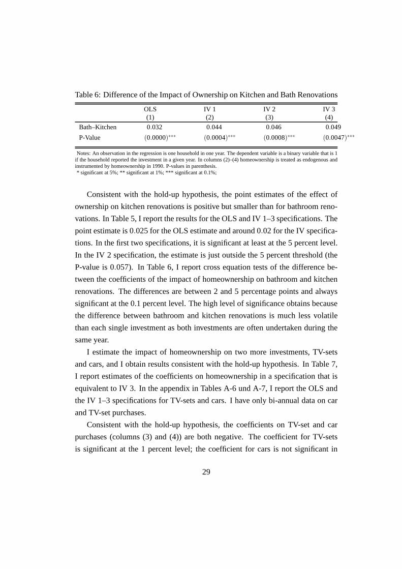
Table 6: Difference of the Impact of Ownership on Kitchen andBath Renovations

OLS IV 1 IV 2 IV 3(1) (2) (3) (4)

Bath–Kitchen 0.032 0.044 0.046 0.049

P-Value (0.0000)∗∗∗ (0.0004)∗∗∗ (0.0008)∗∗∗ (0.0047)∗∗∗

Notes: An observation in the regression is one household in one year. The dependent variable is a binary variable that is 1if the household reported the investment in a given year. In columns (2)–(4) homeownership is treated as endogenous andinstrumented by homeownership in 1990. P-values in parenthesis.* significant at 5%; ** significant at 1%; *** significant at 0.1%;

Consistent with the hold-up hypothesis, the point estimates of the effect of

ownership on kitchen renovations is positive but smaller than for bathroom reno-

vations. In Table 5, I report the results for the OLS and IV 1–3specifications. The

point estimate is 0.025 for the OLS estimate and around 0.02 for the IV specifica-

tions. In the first two specifications, it is significant at least at the 5 percent level.

In the IV 2 specification, the estimate is just outside the 5 percent threshold (the

P-value is 0.057). In Table 6, I report cross equation tests of the difference be-

tween the coefficients of the impact of homeownership on bathroom and kitchen

renovations. The differences are between 2 and 5 percentagepoints and always

significant at the 0.1 percent level. The high level of significance obtains because

the difference between bathroom and kitchen renovations ismuch less volatile

than each single investment as both investments are often undertaken during the

same year.

I estimate the impact of homeownership on two more investments, TV-sets

and cars, and I obtain results consistent with the hold-up hypothesis. In Table 7,

I report estimates of the coefficients on homeownership in a specification that is

equivalent to IV 3. In the appendix in Tables A-6 und A-7, I report the OLS and

the IV 1–3 specifications for TV-sets and cars. I have only bi-annual data on car

and TV-set purchases.

Consistent with the hold-up hypothesis, the coefficients onTV-set and car

purchases (columns (3) and (4)) are both negative. The coefficient for TV-sets

is significant at the 1 percent level; the coefficient for carsis not significant in

29

Table 7: Probability of Investment; IV Estimates for Different Investments

Bath Kitchen Car TV-Set(1) (2) (3) (4)

Homeownership 0.063 0.032 −0.031 −0.047(0.016)∗∗∗ (0.015)∗ (0.018) (0.018)∗∗

Refurbishment 0.023 0.011 −0.00031 0.0081need (0.0067)∗∗∗ (0.0065) (0.0080) (0.0081)

Built −0.023 −0.012 0.024 0.055after reunification (0.0088)∗ (0.010) (0.016) (0.017)∗∗

Income −0.0004 0.0003 0.002 0.002(0.0005) (0.0005) (0.0009)∗ (0.0009)∗

Income −0.001 0.0005 −0.002 0.004from wealth (0.001) (0.002) (0.002) (0.002)

Year Dummies X X X X

N.obs. 4007 4007 3923 3893R2 0.024 0.013 0.003 0.009

Notes: An observation in the regression is one household in one year. The dependent variable is a binary variable thatis 1 if the household reported the investment in a given year.Data on purchases of TV-Sets and cars are available onlybi-annualy; to make the results comparable columns (1) and (2) include only even years for which data on TV-sets and carsis available, too. Homeownership is treated as endogenous and instrumented by homeownership in 1990. Robust standarderrors clustered by household in parenthesis.* significant at 5%; ** significant at 1%; *** significant at 0.1%;

this specification. In the fuller set of specifications, which I report in the ap-

pendix in Tables A-6 und A-7, I find that all point estimates for cars and TV-sets

are negative; the estimates are each significant in two out offour specifications.

The negative coefficients plausibly obtain because households face budget and fi-

nancing constraints. Homeowners spend more on the dwellingspecific parts of

the interior decoration (e.g. bathroom fixtures) but less onmovable items (TV-

sets). They also finance more dwelling specific durables (kitchens) but less other

durables (cars).

As a comparison, I include the data on bathroom and kitchen renovations only

for the (even) years for which I have car and TV-set purchase data. The reduced

sample estimates for bathroom renovations (column (1) of Table 7) are essentially

identical to the full sample results (column (2) of Table 2).The estimate of the

effect of homeownership on kitchen renovations (column (2)of Table 7) is 3.2

percentage points. It is significant at the 5 percent level. This point estimate is

30

somewhat higher than the full sample specifications reported in Table 5.

4.3 East-West Comparison

In this section, I compare the effect of homeownership on relationship specific

investments in East Germany and West Germany. I cannot replicate the natural

experiment for West Germany, but I can compare the OLS estimates with the

significant baseline controls. I construct the West German sample in the same

way as the original sample: I include all households that were in the West German

sample in 1990 and follow them until 2002; i.e., a household that resided in West

Germany in 1990 but moved to East Germany before 1997 is included in the West

German sample. As in the East German sample, I do not include later expansions

of the panel.

The coefficient estimate for West Germany (Table 8 column (2)) is positive and

significant at the 1 percent level. Its magnitude of 1.9 percentage points is smaller

than in the East German sample but still economically significant given that the

mean renovation probability in the West Germany sample (3.2percent) is only

half the mean renovation probability in the East German sample (6.1 percent).

The different mean renovation probabilities reflect the East German catch-up to

West German housing standards.

4.4 The Years 1992–1996

In this section, I repeat my analysis of the effect of homeownership on relation-

ship specific investments in East Germany for the years 1992–1996.14 In these

years, homeownership may have been disputed in some cases. Yet I should find,

nevertheless, some effect of ownership on investment. I include all controls that

were significant in one of the main specifications with the exception of the dummy

for construction after reunification. I cannot construct such a dummy for the early

14I start my analysis with the year 1992 because the questionnaire in 1991 did not record whetherthere was a bathroom renovation.

31

Table 8: Probability of Investment; OLS Estimates for East and West Germany

East Germany West Germany(1) (2)

Homeownership 0.059 0.019(0.0071)∗∗∗ (0.0036)∗∗∗

Refurbishment 0.030 0.016need (0.0051)∗∗∗ (0.0030)∗∗∗

Built −0.020 −0.014after reunification (0.0068)∗∗ (0.0041)∗∗∗

Income −0.0003 0.0003(0.0004) (0.0002)

Income −0.001 −0.0004from wealth (0.001) (0.0005)

Year Dummies X X

N.obs. 8210 17318R2 0.029 0.007

Notes: An observation in the regression is one household in one year. The dependent variable is abinary variable that is 1 if the household reported that its bathroom was renovated in a given year.Robust standard errors clustered by household in parenthesis.* significant at 5%; ** significant at 1%; *** significant at 0.1%;

years because the most recent category of the variable “yearof construction” is

“after 1981”. I include a dummy for these years to control fornew buildings.

In column (2) of Table 9, I present the regression results. The coefficients are

essentially the same as in column (1), i.e., the same relationship between own-

ership and investment holds for the earlier years. The mean yearly renovation

probability (6.8 percent) is also similar for this period compared to the later years.

5 Conclusion

In this paper, I have applied the canonical model of Grossmanand Hart (1986)

to the housing market. Under the assumption that landlords and tenants rely on

ex-post negotiation to share the surplus of relationship specific investments, the

32

Table 9: Probability of Investment; IV Estimates for the years 1997–2002 and1992–1996

1997–2002 1992–1996(1) (2)

Homeownership 0.066 0.062(0.012)∗∗∗ (0.012)∗∗∗

Refurbishment 0.031 0.019need (0.0051)∗∗∗ (0.0049)∗∗∗

Built −0.020after reunification (0.0068)∗∗

Built −0.028after 1981 (0.0067)∗∗∗

Income −0.0004 0.001(0.0004) (0.0007)

Income −0.002 0.006from wealth (0.001) (0.004)

Year Dummies X X

N.obs. 8195 8438R2 0.029 0.027

Notes: An observation in the regression is one household in one year. The dependent variable is abinary variable that is 1 if the household reported that its bathroom was renovated in a given year.Homeownership is treated as endogenous and instrumented byhomeownership in 1990. Robuststandard errors clustered by household in parenthesis.* significant at 5%; ** significant at 1%; *** significant at 0.1%;

model predicts that renovations of fixtures should be less frequent in rented hous-

ing than in owner occupied housing. Empirically, this prediction is borne out by

data from the German housing market. Bathroom renovations are less likely in

rental than in owner occupied housing. I interpret this as evidence for a hold-up

problem in the housing market: Tenants fear that they lose part of the return if

they undertake relationship specific investments. I conclude that, at least in the

German housing market, asset ownership determines relationship specific invests

— just as Grossman and Hart’s (1986) model predicts.

Thus, even though the German housing market is large and mature, mar-

33

ket participants seem to have failed to develop a contract that remedies under-

investment. The modernization agreement solves the hold-up problem only if

the transfer to the tenant can be conditioned on the market value of his invest-

ment. Yet modernization agreements do not routinely include mechanisms that

allow the parties to do just that. As the market value of the investment can be

observed by outsiders, I would argue that this is an instanceof the observable-but-

unverifiable-information problem often cited in support ofthe incomplete con-

tracting paradigm (Bolton and Dewatripont 2005, p. 553).

34

Appendix

Table A-1: Descriptive statistics East German Households 1997–2002.

N. Obs. Mean Std. Dev, Min. Max.

Bath renovation 8351 0.061 0.24 0 1

Kitchen renovation 8351 0.055 0.23 0 1

TV-set purchase 3962 0.11 0.31 0 1Car purchase 3993 0.12 0.32 0 1

Homeownership 8351 0.40 0.49 0 1

Homeownership in 1990 8335 0.29 0.45 0 1

Refurbishment need 8263 1.54 0.66 1 4

Built after reunification 8291 0.12 0.33 0 1

Income 8351 16.7 6.95 0.036 165.5

Income from wealth 8351 1.27 2.33 0 55.0

Wealth 7463 47.1 67.9 −98.0 941.0

Single family home 8300 0.42 0.49 0 1

Distance from city center 7929 3.30 1.49 1 6

Stay for five more years 6725 0.83 0.38 0 1

Age head of household 8351 53.7 13.7 19 97

Children under 18 8351 0.52 0.84 0 5

Notes: An observation is one household in one year for which data on bath renovations is non-missing.

35

Table A-2: Estimates of the Probability of a Bathroom Renovation between 1997 and 2002. Probit and BivariateProbit Estimates.

Probit Bivariate Probit 1 Biv. Probit 2 Biv. Probit 3 Biv. Probit 4(1) (2) (3) (4) (5)

Homeownership 0.48 0.51 0.48 0.53 0.52(0.056)∗∗∗ (0.079)∗∗∗ (0.10)∗∗∗ (0.084)∗∗∗ (0.16)∗∗

Refurbishment 0.25 0.25 0.22 0.25 0.22need (0.038)∗∗∗ (0.039)∗∗∗ (0.041)∗∗∗ (0.039)∗∗∗ (0.044)∗∗∗

Built −0.28 −0.28 −0.29 −0.28 −0.28after reunification (0.091)∗∗ (0.091)∗∗ (0.096)∗∗ (0.091)∗∗ (0.11)∗∗

Income −0.004 −0.004 −0.005 −0.003 −0.003(0.004) (0.004) (0.004) (0.004) (0.005)

Income −0.01 −0.01from wealth (0.01) (0.02)

Wealth −0.0003(0.0005)

Single 0.02family home (0.1)

Distance −0.008from city center (0.02)

Stay for −0.01five more years (0.09)

Age head −0.01of household (0.02)

Age head 0.0001of household2 (0.0002)

Children 0.05under 18 (0.04)

Year Dummies X X X X X

N.obs. 8210 8195 7334 8195 6303R2

Notes: An observation in the regression is one household in one year. The dependent variable is a binary variable that is 1if the householdreported that its bathroom was renovated in a given year. In columns (2)–(5) the effect of homeownership in later years onrenovations inthose years is estimated jointly in a bivariate probit with the effect of homeownership in 1990 on homeownership in lateryears. Robuststandard errors clustered by household in parenthesis.* significant at 5%; ** significant at 1%; *** significant at 0.1%;

36

Table A-3: Estimates of the Marginal Effects of Homeownership on the Probability of a Bathroom Renovationbetween 1997 and 2002. Probit and Bivariate Probit Estimates.

Probit Bivariate Probit 1 Biv. Probit 2 Biv. Probit 3 Biv. Probit 4(1) (2) (3) (4) (5)

Homeownership 0.055 0.058 0.054 0.062 0.060(0.0067)∗∗∗ (0.0100)∗∗∗ (0.012)∗∗∗ (0.011)∗∗∗ (0.021)∗∗

Notes: An observation in the regression is one household in one year. The dependent variable is a binary variable that is 1if the householdreported that its bathroom was renovated in a given year. In columns (2)–(5) the effect of homeownership in later years onrenovations inthose years is estimated jointly in a bivariate probit with the effect of homeownership in 1990 on homeownership in lateryears. Robuststandard errors clustered by household in parenthesis.* significant at 5%; ** significant at 1%; *** significant at 0.1%;

37

Table A-4: Estimates of the Probability of a Bathroom Renovation between 1997and 2002. OLS Estimates with lagged dependent variable.

Bath Residuals

(1) (2) (3)OLS OLS Lag OLS Lag

Homeownership 0.059 0.052 −0.0039(0.0071)∗∗∗ (0.0064)∗∗∗ (0.013)

Refurbishment 0.030 0.032 0.0040need (0.0051)∗∗∗ (0.0048)∗∗∗ (0.0064)

Built −0.020 −0.016 −0.0018after reunification (0.0068)∗∗ (0.0061)∗ (0.0064)

Income −0.00031 −0.00029 −0.00039(0.00042) (0.00038) (0.00038)

Income −0.0013 −0.0013 −0.00013from wealth (0.0010) (0.00096) (0.00098)

Renovationst−1 0.13 −0.071(0.017)∗∗∗ (0.18)

Residualst−1 0.039(0.18)

Residualst−2 0.039(0.028)

Year Dummies X X X

N.obs. 8210 8210 7994R2 0.029 0.048 0.003

Notes: An observation in the regression is one household in one year. In columns (1)–(2) the dependent variable is a binaryvariable that is 1 if the household reported that its bathroom was renovated in a given year. In column (3) the dependentvariable is the residual of the regression in column (2). Robust standard errors clustered by household in parenthesis.* significant at 5%; ** significant at 1%; *** significant at 0.1%;

38

Table A-5: Estimates of the Probability of a Bathroom Renovation between 1997 and 2002 — Only Householdsthat neither moved nor changed their Ownership Status between 1990 and 2002 ; OLS estimates

OLS 1 OLS 2 OLS 3 OLS 4(1) (2) (3) (4)

Homeownership 0.060 0.062 0.059 0.054(0.0086)∗∗∗ (0.0088)∗∗∗ (0.0096)∗∗∗ (0.012)∗∗∗

Refurbishment 0.024 0.024 0.023 0.024need (0.0075)∗∗ (0.0075)∗∗ (0.0075)∗∗ (0.0079)∗∗

Built −0.026 −0.028 −0.023 −0.027after reunification (0.013)∗ (0.013)∗ (0.014) (0.016)

Income −0.0009 −0.0007 −0.001 −0.0005(0.0005) (0.0006) (0.0006) (0.0006)

Income −0.001 −0.001from wealth (0.001) (0.001)

Wealth 0.00003(0.00008)

Single 0.02family home (0.01)

Distance −0.003from city center (0.003)

Stay for −0.03five more years (0.02)

Age head 0.001of household (0.003)

Age head −0.00001of household2 (0.00003)

Children 0.010under 18 (0.007)

Year Dummies X X X X

N.obs. 4882 4882 4751 4185R2 0.027 0.027 0.026 0.028

Notes: An observation in the regression is one household in one year. The dependent variable is a binary variable that is 1if the household reported that its bathroom wasrenovated in a given year. Robust standard errors clusteredby household in parenthesis.* significant at 5%; ** significant at 1%; *** significant at 0.1%;

39

Table A-6: Estimates of the Probability of a TV-set purchasebetween 1998 and 2002 — Bi-annual data.

OLS IV 1 IV 2 IV 3(1) (2) (3) (4)

Homeownership −0.0011 −0.037 −0.047 −0.034(0.010) (0.016)∗ (0.018)∗∗ (0.021)

Refurbishment 0.012 0.0080 0.0081 0.011need (0.0080) (0.0081) (0.0081) (0.0086)

Built 0.054 0.053 0.055 0.060after reunification (0.017)∗∗ (0.017)∗∗ (0.017)∗∗ (0.018)∗∗

Income 0.002 0.002 0.002 0.003(0.0008)∗ (0.0009)∗∗ (0.0009)∗ (0.0009)∗∗

Income 0.004from wealth (0.002)

Wealth 0.00006(0.0001)

Year Dummies X X X X

N.obs. 3900 3893 3893 3568R2 0.013 0.010 0.009 0.014

Notes: An observation in the regression is one household in one year. The dependent variable is a binary variable that is 1if thehousehold reported that it bought a new TV-set in a given year. Data on purchases of TV-sets are available only bi-annualy. In columns(2)–(4) Homeownership is treated as endogenous and instrumented by homeownership in 1990. Robust standard errors clustered byhousehold in parenthesis.* significant at 5%; ** significant at 1%; *** significant at 0.1%;

40

Table A-7: Estimates of the Probability of a car purchase between 1998 and 2002 — Bi-annual data.

OLS IV 1 IV 2 IV 3(1) (2) (3) (4)

Homeownership −0.0060 −0.035 −0.031 −0.040(0.011) (0.017)∗ (0.018) (0.023)

Refurbishment 0.0029 −0.00027 −0.00031 0.0054need (0.0079) (0.0080) (0.0080) (0.0084)

Built 0.026 0.025 0.024 0.030after reunification (0.016) (0.016) (0.016) (0.017)Income 0.001 0.002 0.002 0.002

(0.0008) (0.0008)∗ (0.0009)∗ (0.0009)∗

Income −0.002from wealth (0.002)

Wealth 0.00002(0.0001)

Year Dummies X X X X

N.obs. 3930 3923 3923 3594R2 0.004 0.002 0.003 0.002

Notes: An observation in the regression is one household in one year. The dependent variable is a binary variable that is 1if thehousehold reported that it bought a new car in a given year. Data on purchases of cars are available only bi-annualy. In columns (2)–(4)Homeownership is treated as endogenous and instrumented byhomeownership in 1990. Robust standard errors clustered byhousehold inparenthesis.* significant at 5%; ** significant at 1%; *** significant at 0.1%;

41

Table A-8: Estimates of the Probability of a Bathroom Renovation between 1997 and 2002. OLS Estimates.

(1) (2) (3) (4)OLS 1 OLS 2 OLS 3 OLS 4

Homeownership 0.057 0.059 0.059 0.057(0.0068)∗∗∗ (0.0071)∗∗∗ (0.0076)∗∗∗ (0.0098)∗∗∗

Refurbishment 0.030 0.030 0.026 0.026need (0.0051)∗∗∗ (0.0051)∗∗∗ (0.0053)∗∗∗ (0.0057)∗∗∗

Built −0.019 −0.020 −0.020 −0.021after reunification (0.0068)∗∗ (0.0068)∗∗ (0.0072)∗∗ (0.0087)∗

Income −0.0005 −0.0003 −0.0006 −0.0004(0.0004) (0.0004) (0.0005) (0.0005)

Income −0.001 −0.001from wealth (0.001) (0.001)

Wealth −0.00005(0.00005)

Single 0.004family home (0.009)

Distance −0.0008from city center (0.002)

Stay for 0.0006five more years (0.009)

Age head −0.001of household (0.002)

Age head 0.00001of household2 (0.00002)

Children 0.005under 18 (0.005)

Year Dummies X X X X

N.obs. 8210 8210 7346 6314R2 0.029 0.029 0.028 0.029

Notes: An observation in the regression is one household in one year. The dependent variable is a binary variable that is 1if the householdreported that its bathroom was renovated in a given year. Robust standard errors clustered by household in parenthesis.* significant at 5%; ** significant at 1%; *** significant at 0.1%;

42

References

ALESINA, A., AND N. FUCHS-SCHÜNDELN (2007): “Good Bye Lenin (or Not?):

The Effect of Communism on People’s Preferences,”American Economic Re-

view, 97(4), 1507–1528.

BAKER, G. P., AND T. HUBBARD (2003): “Make or Buy in Trucking: Asset

Ownership, Job Design and Information,”American Economic Review, 93,

551–572.

(2004): “Contractibility and Asset Ownership: On-Board Computers and

Governance un U.S. Trucking,”Quarterly Journal of Economics, 119, 1443–

1479.

BESLEY, T. (1995): “Property Rights and Investment Incentives: Theory and

Evidence from Ghana,”The Journal of Political Economy, 103(5), 903–937.

BOLTON, P., AND M. DEWATRIPONT (2005):Contract theory. MIT Press Cam-

bridge, Mass.

BUCK, H. F. (2004):Mit hohem Anspruch gescheitert — Die Wohnungspolitik

der DDR. Lit Verlag.

BUNDESMINISTERIUM FÜR INNERDEUTSCHE BEZIEHUNGEN (ed.) (2000):

DDR Handbuch. DIRECTMEDIA Publishing GmbH.

CROCKER, K. J., AND K. J. REYNOLDS (1993): “The Efficiency of Incomplete

Contracts: An Empirical Analysis of Air Force Engine Procurement,”Rand

Journal of Economics, 24, 126–146.

FIELD , E. (2005): “Property rights and investment in urban slums,” Journal of

the European Economic Association, 3(2-3), 279–290.

FIELD , E. (2007): “Entitled to Work: Urban Property Rights and Labor Supply

in Peru,”Quarterly Journal of Economics, 122(4), 1561–1602.

43

FUCHS-SCHÜNDELN, N., AND M. SCHÜNDELN (2005): “Precautionary Savings

and Self-Selection: Evidence From the German ReunificationExperiment,”

Quarterly Journal of Economics, 120, 1085–1120.

GROSSMAN, S. J.,AND O. D. HART (1986): “The Costs and Benefits of Owner-

ship: A Theory of Vertical and Lateral Integration,”Journal of Political Econ-

omy, 94(4), 691–719.

HERBST, A., W. RANKE , AND J. WINKLER (eds.) (1994):So funktionierte

die DDR. Lexikon der Organisationen und Institutionen.Rowohlt Taschenbuch

Verlag.

HOFFMANN, M. (1972):Wohnungspolitik der DDR — das Leistungs- und Inter-

essenproblem. Verlag Deutsche Wohnungswirtschaft GmbH.

HÄUSSERMANN, H., B. GLOCK, AND C. KELLER (2000): “Eigentumsstrukturen

zwischen Persistenz und Wandel: Zu den Folgen der Restitution in suburbanen

und innerstädtischen Gebieten,” Working Paper No.5. Plymouth: Media Ser-

vices.

JACOBY, H. G., AND G. MANSURI (2008): “Land Tenancy and Non-Contractible

Investment in Rural Pakistan,”Review of Economic Studies, forthcoming.

LERNER, J., AND U. MALMENDIER (2005): “Contractibility and the Design of

Research Agreements,” NBER Working Paper 11292.

LÜTZENKIRCHEN, K. (ed.) (2003):Anwaltshandbuch Mietrecht. Verlag Dr. Otto

Schmidt, Köln.

REDDING, S., AND D. STURM (2008): “The Costs of Remoteness: Evidence

from German Division and Reunification,”American Economic Review, forth-

coming.

STAIGER, D., AND J. STOCK (1997): “Instrumental Variables Regression with

Weak Instruments,”Econometrica, 65, 557–586.

44

WAGNER, G. G., J. R. FRICK, AND J. SCHUPP (2007): “The German Socio-

Economic Panel Study (SOEP) — Scope, Evolution and Enhancements,”

Schmollers Jahrbuch, 127, 139–169.

WILLIAMSON , O. (1975):Markets and Hierarchies: Analysis of Antitrust Impli-

cations. Free Press, New York.

WOODRUFF, C. (2002): “Non-contractible investments and vertical integration in

the Mexican footwear industry,”International Journal of Industrial Organiza-

tion, 20(8), 1197–1224.

WOOLDRIDGE, J. (2002): Econometric Analysis of Cross Section and Panel

Data. MIT Press.

45