does order matter - nato-us.orgnato-us.org/analysis2000/papers/korner.pdf · does order matter t....

103

Does Order Matter

T. W. Korner

DPMMS16 Mill LaneCambridge

[email protected]

ABSTRACT. I describe the work of Olevskiı, Tao and others on the rearrangement oforthogonal series. It turns out that arbitrary rearrangements produce trouble for allorthogonal and wavelet methods, that decreasing rearrangements produce trouble forFourier series, but that wavelet expansions continue to work well under decreasingrearrangement.

1. Introduction

In this paper we shall move without comment between the circle T = R=Z, the closedinterval [0; 1] and the half closed interval [0; 1) as seems most convenient. When our resultsdeal with almost everywhere behaviour this does not create any problems, when we wanteverywhere convergence readers may have to produce their own argument to deal with thepoint 1.

What do we mean when we consider1X

u=�1

f(u) exp 2�iut ?

Traditionally we take

limN!1

NXu=�N

f(u) exp 2�iut

and the only variations that we allow concern the mode of convergence (pointwise, Lp, etc). Asign that this may be too narrow an approach appears when we consider the two dimensionalcase of a function f : T2 ! C . The obvious way to proceed is to takeX

(u;v)2Z2

f(u; v) exp 2�i(ut+ vs) = limN!1

X(u;v)2�(N)

f(u; v) exp 2�i(ut+ vs)

104 T.W. Korner / Does Order Matter

with the �(N) finite subsets of Z2 such that �(1) � �(2) � : : : andS1

N=1 �(N) = Z2.

However, it is well known that, even when f is quite well behaved, different choices of thesequence �(N) give rise to different behaviour.

The question of ‘correct order’ also arises, even in the one dimensional case, from signalprocessing. If we seek to store and reconstruct a function f : T ! C by using its Fouriercoefficients it is natural to to use them in decreasing order of magnitude and to considerX

jf(u)j>�

f(u) exp 2�iut

rather than Xjuj6N

f(u) exp iut:

Any easy optimism about rearrangements is quenched by the following result.

THEOREM 1. There exists a real f 2 L2(T) and a bijection � : Z! Z such that

lim supN!1

��NX

u=�N

f(�(u)) exp i�(u)t

�� =1:

for almost all t 2 T.

This theorem was first stated by Kolmogorov. A proof of Kolmogorov’s statement wassketched by Zahorskiı, given in detail by Ulyanov and much simplified by Olevskiı. Thereader who consults [7] will find an excellent bibliography.

Polya says that sometimes the easiest way to prove a result is to generalise it and provethe generalisation. By the time Kolmogorov’s theorem reached Ulyanov and Olevskiı it hadtaken the following form.

THEOREM 2. Let �1, �2, �3, . . . form a complete orthonormal system in L2([0; 1)). Thenthere exists a real f 2 L2(T) and a bijection � : N ! N such that

lim supN!1

��NXu=0

f(�(u))��(u)(t)

�� =1:

for almost all t 2 [0; 1).

Here as usual we write

f(�r) = hf; �ri =

Z 1

0

f(t)�r(t) dt:

In fact Olevskiı improved Theorem 2 by replacing f 2 L2(T) by f continuous. We shallprove a result which includes this as Theorem 5.

In the years since Olevskiı published his result, more general systems than those of com-plete orthonormal type have assumed practical importance.

T.W. Korner / Does Order Matter 105

DEFINITION 3. We say that�1; �2; �3; : : :

form a Riesz basis for L2([0; 1)) if the linear span of the �n is dense in L2 and there exists anA with A > 1 such that

A�11Xn=0

janj26

1Xn=0

an�n

2

2

6 A1Xn=0

janj2:

We callA the Riesz constant of the system. Easy functional analysis reveals the followinglemma.

LEMMA 4. Let �1, �2, �3, . . . form a Riesz basis for L2([0; 1)). Then there exists a uniquesequence 1, 2, 3, . . . of bounded L2 norm such that

P1

n=0 jh n; fij2 <1 and

f =

1Xn=0

h n; fi�n

for every f 2 L2: If f =P

1

n=0 an�n then an = h n; fi for all n.

We write f(n) = h n; fi.As Olevskiı indicates very clearly his method can be extended to Riesz bases.

THEOREM 5. Let �1, �2, �3, . . . form a Riesz basis for L2([0; 1]). Then there exists a realcontinuous f and a bijection � : N ! N such that

lim supN!1

��NXu=0

f(�(u))��(u)(t)

�� =1:

for almost all t 2 [0; 1].

If we ask for which complete orthonormal system Theorem 2 is least plausible one answerwould be the Haar system. Set

�(N) = f(r; s) 2 Z2 : 0 6 s 6 2r � 1 and N > r > 0g

and � =S

N>0 �(N). Consider intervals of the form

E(r; s) = [s2�r; (s+ 1)2�r)

where (r; s) 2 �. We define

�r;s(t) = 1 if t 2 E(r + 1; 2s)

�r;s(t) = �1 if t 2 E(r + 1; 2s+ 1)

�r;s(t) = 0 otherwise

where, again, (r; s) 2 �. We call the �r;s together with the function 1 = ��1;0 the Haarsystem. We call the Tr;s = 2r=2�r;s together with the function 1 the normalised Haar system.


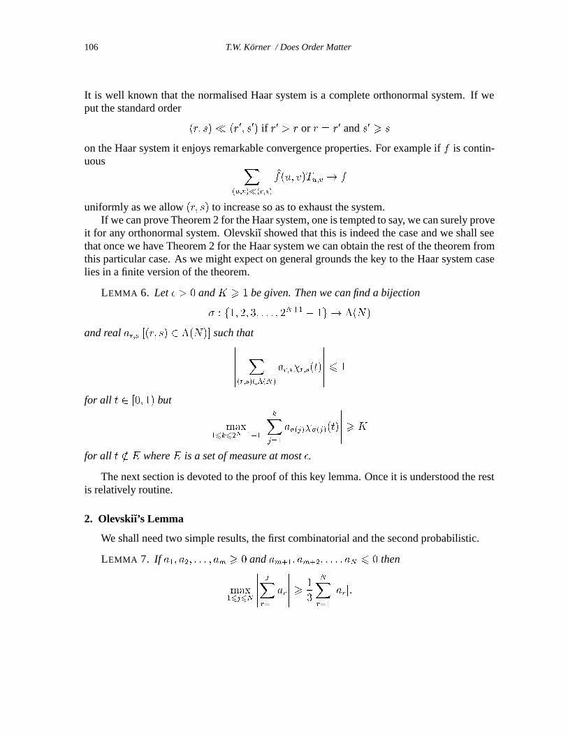
It is well known that the normalised Haar system is a complete orthonormal system. If weput the standard order

(r; s)� (r0; s0) if r0 > r or r = r0 and s0 > s

on the Haar system it enjoys remarkable convergence properties. For example if f is contin-uous X

(u;v)�(r;s)

f(u; v)Tu;v ! f

uniformly as we allow (r; s) to increase so as to exhaust the system.If we can prove Theorem 2 for the Haar system, one is tempted to say, we can surely prove

it for any orthonormal system. Olevskiı showed that this is indeed the case and we shall seethat once we have Theorem 2 for the Haar system we can obtain the rest of the theorem fromthis particular case. As we might expect on general grounds the key to the Haar system caselies in a finite version of the theorem.

LEMMA 6. Let � > 0 and K > 1 be given. Then we can find a bijection

� : f1; 2; 3; : : : ; 2N+1� 1g ! �(N)

and real ar;s [(r; s) 2 �(N)] such that��X

(r;s)2�(N)

ar;s�r;s(t)

�� 6 1

for all t 2 [0; 1) but

max16k62N+1�1

��kX

j=1

a�(j)��(j)(t)

�� > K

for all t =2 E where E is a set of measure at most �.

The next section is devoted to the proof of this key lemma. Once it is understood the restis relatively routine.

2. Olevskiı’s Lemma

We shall need two simple results, the first combinatorial and the second probabilistic.

LEMMA 7. If a1; a2; : : : ; am > 0 and am+1; am+2; : : : ; aN 6 0 then

max16j6N

��jX

r=1

ar

�� > 1

3

NXr=1

jarj:


PROOF. Observe thatNXr=1

jarj = 2

mXr=1

ar �NXr=1

ar 6 3 max16j6N

��jX

r=1

ar

�� :

LEMMA 8. Let X1, X2, . . . , XN be independent identically distributed random variableswith Pr(Xr = 1) = Pr(Xr = �1) = 1=2 and let K be an integer with K > 1. Then

(i) Pr�max16j6N

Pj

r=1Xr > K�6 2Pr

�PN

r=1Xr > K�:

(ii) Pr�max16j6N

��Pj

r=1Xr

�� > K�6 4Pr

��PN

r=1Xr

�� > K�:

(iii) Pr�max16j6N

��Pj

r=1Xr

�� > K�6 2NK�2:

PROOF. (i) This is the simplest form of the reflection principle. (See e.g. [2] Chap-ter 3.)

(ii) Use symmetry.

(iii) Use Chebychev’s inequality to bound Pr��PN

r=1Xr

�� > K�

.

Of course, we can get much better estimates in (iii) but the only use I can find for suchestimates is to study the Hausdorff dimension of the exceptional set of convergence in Theo-rem 2 when applied to Haar functions.

By using the standard interpretation of Haar functions in terms of coin tossing, Lemma 8gives the following result.

LEMMA 9. IfN andK are strictly positive integers then we can find ap;q taking the values0 or 1 [(p; q) 2 �(N)] and a set E of measure at most 4NK�2 such that��

X(p;q)2�(N)

ap;q�p;q(t)

�� 6 K

for all t 2 [0; 1), but X(p;q)2�(N)

jap;q�p;q(t)j = N

for all t =2 E.

PROOF. Consider [0; 1) with Lebesgue measure as a probability space. Let

Xj(t) = (�1)[2jt]


(where [2jt] is the integer part of 2jt). The Xj satisfy the conditions of Lemma 8. It followsby Lemma 8 (iii) that the set

E =

(t : max

16j6N

��jX

r=1

Xr

�� > K

)

has measure at most 4NK�2.To define ap;q we look at the interval E(p; q) = [p2�q; (p + 1)2�q) and observe thatP

j

r=1Xr(t) is constant on E(p; q) for all 1 6 j 6 q � 1. We may thus define ap;q = 1 if

max16j6N

��jX

r=1

Xr(t)

�� 6 K � 1

for t 2 E(p; q), and ap;q = 0 otherwise.If we now set

Y (t) =X

(p;q)2�(N)

ap;q�p;q(t)

then Y is the random variable defined by

Y (t) =NXr=1

Xr(t)

if jmax16j6NP

j

r=1Xr(t)j 6 K but

Y (t) =

j(t)Xr=1

Xr(t)

where j(t) is the smallest j with jP

j(t)r=1Xr(t)j = K. In more vivid terms, toss a fair coin

keeping track of the difference between the number of heads and tails thrown. If this evertakes the value K or �K stop and record the value as Y . If, after N throws this has nothappened, record the value after N throws as Y . By definition jY (t)j 6 K and if t =2 E (sowe complete the N throws) X

(p;q)2�(N)

jap;q�p;q(t)j = N

as required.

Now, instead of taking the sequence of heads and tails as chance presents them, we wishto take all the heads first and then all the tails. To do this we introduce the Olevskiı order on�

(p0; q0) � (p; q) if (2p0 + 1)2�q0

> (2p+ 1)2�q:


The Olevskiı order is more intricate than may at first appear and the reader should try orderingthe (p; q) with (p; q) 2 �(N) for N = 5 or N = 6. Observe that (p0; q0) � �(p; q) if the mid-point of supp�p0;q0 is to the right of (i.e. greater than or equal to) the mid-point of supp�p;q.We observe that �p;q(t) > 0 if t is strictly to the left of (i.e. strictly less than) the mid-pointof supp�p;q and �p;q(t) 6 0 if t is to the right of (i.e. greater than or equal to) the mid-pointof supp�p;q. It follows that for each t 2 [0; 1) there is a �(t) 2 �(N) such that

�p;q(t) 6 0 for� � (p; q); �p;q(t) > 0 for(p; q) � ��:

Using this observation we easily arrive at the result we require.

LEMMA 10. Suppose that N and K are strictly positive integers and ap;q and E are as inLemma 9. Then

max�2�(N)

��X

��(p;q)

ap;q�p;q(t)

�� > N=3

for all t =2 E.

PROOF. By Lemma 7 and the last sentence of the previous paragraph

max�2�(N)

��X� � (p; q)ap;q�p;q(t)�� > 1

3

X(p;q)2�(N)

jap;q�p;q(t)j = N=3

for all t =2 E.

THEOREM 11. Let � > 0 and � > 1 be given. Then we can find an N > 1, 1 > b > 0,bp;q taking the values 0 or b [(p; q) 2 �(N)] and a set E such that

(i) jP

(p;q)2�(N) bp;q�p;q(t)j 6 1 for all t 2 [0; 1),(ii) max�2�(N) j

P��(p;q) ap;q�p;q(t)j > � for all t =2 E

(iii) jEj < �.

PROOF. Choose an integer M with M > 4��1 and M2 > 3�. Set N = M5, K = M3

and choose ap;q and E as in Lemma 9. If we now put bp;q = ap;q=K, b = 1=K then all theconclusions of the lemma with the exception of condition (ii) follow at once from Lemma 9.Condition (ii) itself follows from Lemma 10.

Standard ‘rolling hump’ (or ‘condensation of singularities’) methods now give the fol-lowing result.

EXERCISE 12. Let �n [n 2 N ] be the Haar system enumerated in some way. Then thereexists a real f 2 L1([0; 1)) and a bijection � : N ! N such that

lim supN!1

��NXu=0

f(�(u))��(u)(t)

�� =1:

for almost all t 2 [0; 1).


We leave it as an exercise for the reader because we shall prove stronger results. Howeverthese results will require extra complications in their proofs and the reader may find the morecomplex proofs easier to follow if he or she has worked through an easier case.

3. Extension To General Spaces

We have not yet exhausted the strength of Polya’s dictum. What happens if we seek toextend Theorem 2 to more general measure spaces? A moment’s reflection brings to mindthe the fact that, so far as measure theory is concerned, all nice measure spaces which arenot obviously different are the same. Recall that a measure space (X;F ; �) with positivemeasure � is non-atomic if givenE 2 F with �(E) > 0 we can find F 2 F with F � E and�(E) > �(F ) > 0. The following result is typical (see e.g. theorem 9, page 327 of [8]).

THEOREM 13. Let X be a complete separable metric space equipped with BX its �-algebra of Borel sets and � a non-atomic measure on BX . If I = [0; 1] is the unit intervalwith its usual metric, BI its �-algebra of Borel sets, and m is the usual Lebesgue measurethen there exists a bijective map F : I ! X such that F and F �1 carry Borel sets to Borelsets of the same measure.

We shall not use Theorem 13 but we shall use the lemma which underlies its proof andthe proof of results like it.

LEMMA 14. Let (X;F ; �) be a non-atomic probability space. If E 2 F and 1 > � > 0then we can find F 2 F with E � F and �(F ) = ��(E).

Lemma 17 follows easily from a lemma of Saks given as Lemma 7 of section IV.9.8 ofDunford and Schwartz [1]. There is a discussion of isomorphism theorems in Chapter VIII ofHalmos’s Measure Theory [3]. However before readers rush off to inspect the wilder shoresof measure theory they should note that all they will learn is that they could have stayed athome, since [0; 1] with Lebesgue measure is the type of all non-atomic measure spaces.

In view of the preceding discussion, it is natural to aim at the following generalisation ofTheorem 2. (The extension of Definition 3 to general probability spaces is obvious.)

THEOREM 15. Let (X;F ; �) be a probability space with � non-atomic. Let �1, �2, . . . bea Riesz basis in L2(X). Then there exists a real f 2 L2(X) and a bijection � : N ! N suchthat

lim supN!1

��NXu=0

f(�(u))��(u)(t)

�� =1:

for almost all t 2 X .

The result is clearly false if � is not non-atomic. Suppose E 2 F is an atom, that is�(E) > 0 and if F 2 F with F � E then �(F ) = �(E) or �(F ) = 0. Then if gn; g 2 L2(X)and jjgn � gjj2 ! 0 it follows that gn(t)! g(t) for �-almost all t 2 E.


It is not hard to obtain Theorem 15 from Theorem 2 by the standard argument used toprove results like Theorem 13. However, it is more interesting to ask how we might tackleTheorem 15 directly and, in particular, what we are to make of Theorem 11 in the generalcontext. If we do so we are rewarded with a key insight — Theorem 11 is a combinatorialtheorem.

THEOREM 16. Let (X;F ; �) be a probability space. Let � > 0 and � > 1 be given. Thenwe can find an N > 1, 1 > b > 0 and bp;q taking the values 0 or b [(p; q) 2 �(N)] with thefollowing property.

Suppose that we have a collection of sets En;r 2 F such that

(A) E(2r � 1; n+ 1) \ E(2r; n+ 1) = ;, E(2r� 1; n+ 1) [ E(2r; n+ 1) = E(r; n) forall (r; n) 2 �N .

(B) jE(r; n)j = 2�n for all (r; n) 2 �N+1.

Let us set

Hr;n(t) = 1 for t 2 E(2r � 1; n+ 1),

Hr;n(t) = �1 for t 2 E(2r; n+ 1),

Hr;n(t) = 0 otherwise.

whenever (r; n) 2 �N . Then(i) j

P(p;q)2�(N) bp;qHp;q(t)j 6 1 for all t 2 [0; 1),

and there is a set E 2 F such that(ii) max�2�(N) j

P��(p;q) bp;qHp;q(t)j > � for all t =2 E

(iii) jEj < �.

PROOF. This is just Theorem 11.

To see why this is indeed an insight let us return to the concrete case of Lebesgue mea-sure on [0; 1) and consider the most important Riesz basis of all, the exponentials en(t) =exp(2�int). If we try to convert Theorem 11 into a result on Fourier series we run into theproblem that different Haar functions do not ‘occupy different parts of the frequency spec-trum’. (Indeed the Fourier coefficients of the Haar functions �p;q with fixed p are all of sameamplitude differing only in phase.) However, if we ‘shuffle [0; 1)’ the Ep;q can be chosen sothat the Hp;q are, for practical purposes, in ‘different parts of the frequency spectrum’. Thatis, although we do not have the ideal outcome in which at most one of the Hp;q(j) is non-zerofor each j, we can arrange that at most one of the Hp;q(j) is large for each j.

Since there seems no further advantage in considering general measure spaces we shallstay within [0; 1) and [0; 1]. However, readers who wish to work more generally will find thatthey only need the following simple consequence of Lemma 14.

LEMMA 17. Let (X;F ; �) be a non-atomic probability space. If F 2 F and �(F ) > 0we can find a sequence ej of orthogonal functions and sets Fj 2 F with Fj � F such that


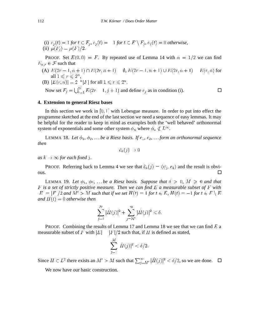
(i) ej(t) = 1 for t 2 Fj , ej(t) = �1 for t 2 F n Fj, ej(t) = 0 otherwise,(ii) �(Fj) = �(F )=2.

PROOF. Set E(0; 0) = F . By repeated use of Lemma 14 with � = 1=2 we can findEn;r 2 F such that

(A) E(2r � 1; n+ 1) \ E(2r; n+ 1) = ;, E(2r� 1; n+ 1) [E(2r; n+ 1) = E(r; n) forall 1 6 r 6 2n,

(B) jE(r; n)j = 2�njF j for all 1 6 r 6 2n.

Now set Fj =S2j

r=1E(2r � 1; j + 1) and define ej as in condition (i).

4. Extension to general Riesz bases

In this section we work in [0; 1] with Lebesgue measure. In order to put into effect theprogramme sketched at the end of the last section we need a sequence of easy lemmas. It maybe helpful for the reader to keep in mind as examples both the ‘well behaved’ orthonormalsystem of exponentials and some other system �n where �n =2 L1.

LEMMA 18. Let �1, �2, . . . be a Riesz basis. If e1, e2, . . . form an orthonormal sequencethen

ek(j)! 0

as k !1 for each fixed j.

PROOF. Referring back to Lemma 4 we see that ek(j) = h j; eki and the result is obvi-ous.

LEMMA 19. Let �1, �2, . . . be a Riesz basis. Suppose that Æ > 0, M > 0 and thatF is a set of strictly positive measure. Then we can find E a measurable subset of F withjEj = jF j=2 and M 0 > M such that if we set H(t) = 1 for t 2 E, H(t) = �1 for t 2 F n Eand H(t) = 0 otherwise then

MXj=1

jH(j)j2 +1X

j=M 0

jH(j)j2 < Æ:

PROOF. Combining the results of Lemma 17 and Lemma 18 we see that we can find E ameasurable subset of F with jEj = jF j=2 such that, if H is defined as stated,

MXj=1

jH(j)j2 < Æ=2:

Since H 2 L2 there exists an M 0 > M such thatP

1

j=M 0 jH(j)j2 < Æ=2, so we are done.

We now have our basic construction.


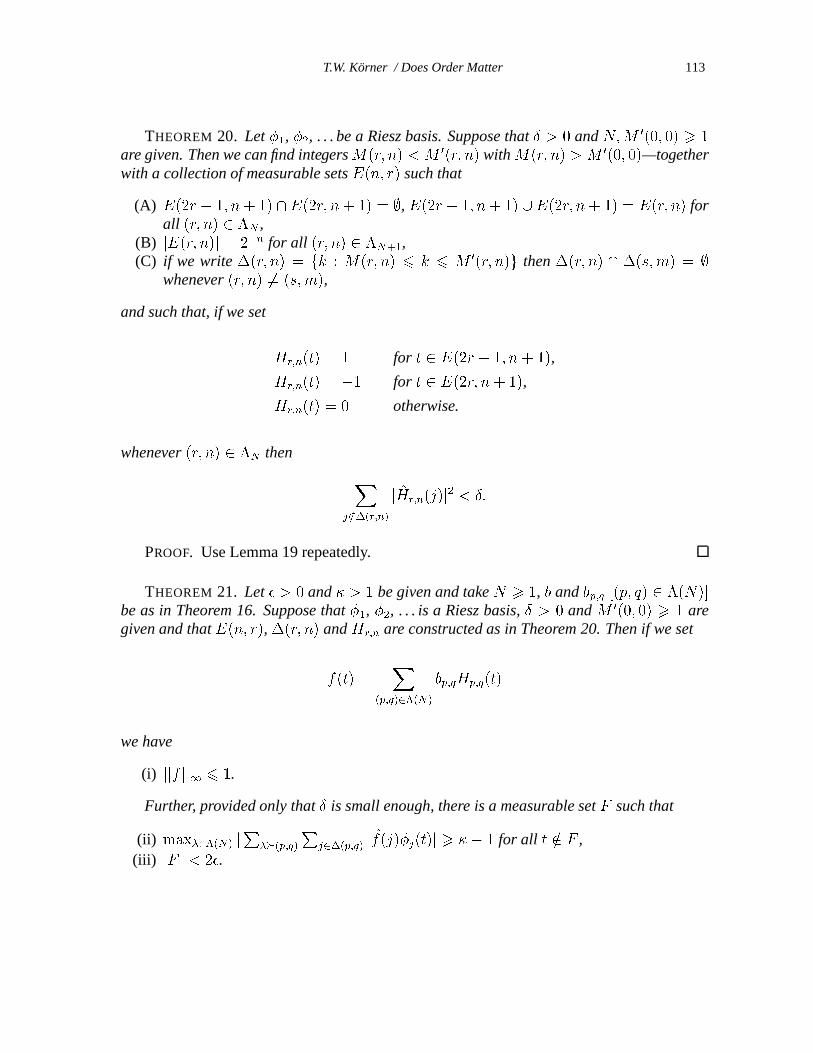
THEOREM 20. Let �1, �2, . . . be a Riesz basis. Suppose that Æ > 0 and N;M 0(0; 0) > 1are given. Then we can find integersM(r; n) < M 0(r; n) with M(r; n) > M 0(0; 0)—togetherwith a collection of measurable sets E(n; r) such that

(A) E(2r � 1; n+ 1) \ E(2r; n+ 1) = ;, E(2r� 1; n+ 1) [ E(2r; n+ 1) = E(r; n) forall (r; n) 2 �N ,

(B) jE(r; n)j = 2�n for all (r; n) 2 �N+1,(C) if we write �(r; n) = fk : M(r; n) 6 k 6 M 0(r; n)g then �(r; n) \ �(s;m) = ;

whenever (r; n) 6= (s;m),

and such that, if we set

Hr;n(t) = 1 for t 2 E(2r � 1; n+ 1),

Hr;n(t) = �1 for t 2 E(2r; n+ 1),

Hr;n(t) = 0 otherwise.

whenever (r; n) 2 �N then

Xj =2�(r;n)

jHr;n(j)j2 < Æ:

PROOF. Use Lemma 19 repeatedly.

THEOREM 21. Let � > 0 and � > 1 be given and take N > 1, b and bp;q [(p; q) 2 �(N)]be as in Theorem 16. Suppose that �1, �2, . . . is a Riesz basis, Æ > 0 and M 0(0; 0) > 1 aregiven and that E(n; r), �(r; n) and Hr;n are constructed as in Theorem 20. Then if we set

f(t) =X

(p;q)2�(N)

bp;qHp;q(t)

we have

(i) jjf jj1 6 1.

Further, provided only that Æ is small enough, there is a measurable set F such that

(ii) max�2�(N) jP

��(p;q)

Pj2�(p;q) jf(j)�j(t)j > �� 1 for all t =2 F ,

(iii) jF j < 2�.


PROOF. Conclusion (i) is just conclusion (i) of Theorem 20. To obtain (ii) and (iii) weproceed as follows. Observe that

X��(p;q)

Xj2�(p;q)

f(j)�j �X

��(p;q)

bp;qHp;q

2

6X

��(p;q)

jbp;qjX

j2�(p;q)

Hp;q �X

j2�(p;q)

f(j)�j

2

6X

��(p;q)

Xj2�(p;q)

Hp;q �X

j2�(p;q)

f(j)�j

2

:

But, for each (p; q) 2 �(N), Hp;q �X

j2�(p;q)

f(j)�j

2

6

X

j =2�(p;q)

Hp;q(j)�j

2

+X

(r;s)6=(p;q)

X

j2�(p;q)

Hr;s(j)�j

2

6

X

j =2�(p;q)

Hp;q(j)�j

2

+X

(r;s)6=(p;q)

X

j =2�(r;s)

Hr;s(j)�j

2

=X

(r;s)2�(N)

X

j =2�(r;s)

Hr;s(j)�j

2

:

But, writing A for the Riesz constant of the basis, Theorem 20 tells us that X

j =2�(r;s)

Hr;s(j)�j

2

2

6 AX

j =2�(r;s)

jHr;s(j)j2 < AÆ:

Thus, retracing our steps, Hp;q �X

j2�(p;q)

f(j)�j

2

< 2N(AÆ)1=2


and X

��(p;q)

Xj2�(p;q)

f(j)�j �X

��(p;q)

bp;qHp;q

2

< 22N(AÆ)1=2

for all � 2 �(N).If we now write

F� =

8<:t :

��X

��(p;q)

Xj2�(p;q)

f(j)�j �X

��(p;q)

bp;qHp;q

�� > 1

9=; ;

then Chebychev’s inequality and the last inequality of the preceding paragraph tell us that

jF�j < 24NAÆ:

Thus if we set F = E [S

�2�(N) F� conclusion (ii) follows from conclusion (ii) Theorem 20whilst conclusion (iii) Theorem 20 tells us that

jF j < � + 25NAÆ;

and (iii) holds provided only that Æ is small enough.

Theorems 20 and 21 give us what we want. However, we have accumulated a fair amountof notation in the course of the construction which we can now jettison to provide a simplerconclusion.

THEOREM 22. Let �1, �2, . . . be a Riesz basis. Given K > 1 we can find an integerM(K) > 1 with the following properties. Given any integer m > 1 and any � > 0 we canfind a function f 2 L1([0; 1]), an integer m0 > m, a bijection � : N ! N with �(r) = rfor 1 6 r 6 m and for r > m0, integers m 6 p(1) 6 p(2) 6 p(3) : : : p(M) 6 m0 and ameasurable set E such that

(i) jjf jj1 6 1,(ii)

Pm

j=1 jf(j)j2 6 �,

(iii) max16k6M jP

p(k)j=1 f(�(j))��(j)j > K for all t 2 E,

(iv) jEj > 1�K�1.

The distance from L1([0; 1]) to C([0; 1]) is usually not very great. The present case is noexception.

THEOREM 23. In Theorem 22 we may take f continuous.

PROOF. This is entirely routine. Let the M(K) of our new Theorem 23 be chosen to bethe M(2K + 2) of the old Theorem 22. Then, by Theorem 22, given any m > 1 and any� > 0 we can find a function f 2 L1([0; 1)), an integer m0 > m, a bijection � : N ! N with�(r) = r for 1 6 r 6 m and for r > m0, integers m 6 p(1) 6 p(2) 6 p(3) : : : p(M) 6 m0

and a measurable set E 0 such that


(i) 0 jjf jj1 6 1,(ii) 0

Pm

j=1 jf(j)j2 6 �,

(iii) 0 max16k6M jP

p(k)j=1 f(�(j))��(j)(t)j > K + 1 for all t 2 E,

(iv) 0 jE 0j > 1�K�1=2.

Let Æ > 0 be a small number to be determined and choose f 2 C([0; 1)) such that f satisfiescondition (i) and jjf � gjj2 6 Æ=A2. Automatically

1Xj=1

jf(j)� g(j)j2

!1=2

6 Æ=A

so condition (ii) is satisfied provided only that we choose Æ small enough.Next we observe that

p(k)Xj=1

f(j)�j �

p(k)Xj=1

g(j)�j

2

6 A

0@p(k)X

j=1

jf(j)� g(j)j2

1A

1=2

6 A

1Xj=1

jf(j)� g(j)j2

!1=2

6 Æ:

Thus writing

Ek =

8<:t 2 [0; 1) :

p(k)Xj=1

f(j)�j �

p(k)Xj=1

g(j)�j

> 1

9=; ;

we have, by Chebychev’s inequality,

jEkj 6

p(k)Xj=1

f(j)�j �

p(k)Xj=1

g(j)�j

2

= Æ:

Thus, setting E = E 0 nS

N

k=1, we see that (iii) holds automatically and

jEj > jE 0j �

NXk=1

jEkj > (1� �=2)�NÆ

so that (iv) holds provided only that we choose Æ small enough.

The remainder of the construction follows a standard rolling hump (condensation of sin-gularities) pattern using Chebychev’s inequality in the same way as in the two previousproofs. In view of the amount of notation involved readers will probably prefer to do itthemselves rather than follow my proof.

It is easy to put the bricks of Theorem 23 together.


LEMMA 24. Let �1, �2, . . . be a Riesz basis with constant A. Let m0(0) = 1 We can con-struct inductively positive integers M(n), m(n), m0(n) with m0(n � 1) < m(n), continuousfunctions fn, bijections �n : N ! N with �n(r) = r for 1 6 r 6 m0(n�1) and form0(n) 6 r,integers m 6 p(1; n) 6 p(2; n) 6 p(3; n) : : : p(n;M(n)) 6 m0 and a measurable set E suchthat

(i) n jjfnjj1 6 2�n,(ii) n

Pm(n)r=1 jfn(r)j

2 6 A�12�4n�4m(n)2,(iii) n max16k6M(n) j

Pp(k;n)j=1 fn(�(j))��n(j)(t)j > 2n for all t 2 E,

(iv) n jEnj > 1� 2�n,(v) n

Pn

j=1

P1

r=m0(n) jfj(r)j2 6 A�12�2n�4M(n + 1)�2.

PROOF. Conditions (i)n to (iv)n come directly from Theorem 23. The key point is thatTheorem 23 allows us to define M(n+ 1) before we define m0(n) in such a way as to satisfycondition (v)n.

PROOF OF THEOREM 5. As I said above, this is routine. It is easy to check that �(r) =�n(r) for m0(n � 1) 6 r 6 m0(n) gives a well defined bijection � : N ! N . By theconditions (i)n gn =

Pn

r=1 fr converges uniformly to a continuous function f as n ! 1.Trivially

��p(k;n)Xj=1

f(�(j))��(j)(t)�

p(k;n)Xj=1

fn(�(j))��(j)(t)

�� 6 kgn�1k1 + jGk;n(t)j

6 1 + jGk;n(t)j;

where

Gk;n(t) =n�1Xr=1

1Xj=p(k;n)+1

fr(�(j))��(j)(t) +1X

r=n+1

p(k;n)Xj=1

fr(�(j))��(j)(t):


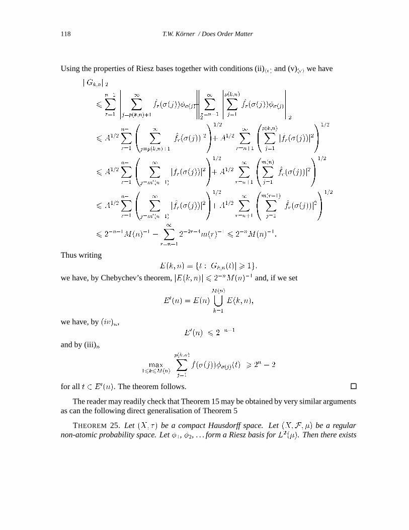
Using the properties of Riesz bases together with conditions (ii)(r) and (v)(r) we have

kGk;nk2

6

n�1Xr=1

1X

j=p(k;n)+1

fr(�(j))��(j)

2

+

1Xr=n+1

p(k;n)Xj=1

fr(�(j))��(j)

2

6 A1=2

n�1Xr=1

0@ 1X

j=p(k;n)+1

jfr(�(j))j2

1A

1=2

+ A1=2

1Xr=n+1

0@p(k;n)X

j=1

jfr(�(j))j2

1A

1=2

6 A1=2

n�1Xr=1

0@ 1X

j=m0(n�1)

jfr(�(j))j2

1A

1=2

+ A1=2

1Xr=n+1

0@m(n)X

j=1

jfr(�(j))j2

1A

1=2

6 A1=2

n�1Xr=1

0@ 1X

j=m0(n�1)

jfr(�(j))j2

1A

1=2

+ A1=2

1Xr=n+1

0@m(r�1)X

j=1

jfr(�(j))j2

1A

1=2

6 2�n�1M(n)�1 +1X

r=n+1

2�2r�4m(r)�1 6 2�nM(n)�1:

Thus writingE(k; n) = ft : jGk;n(t)j > 1g;

we have, by Chebychev’s theorem, jE(k; n)j 6 2�nM(n)�1 and, if we set

E 0(n) = E(n)

M(n)[k=1

E(k; n);

we have, by (iv)n,jE 0(n)j 6 2�n+1

and by (iii)n

max16k6M(n)

��p(k;n)Xj=1

f(�(j))��(j)(t)

�� > 2n � 2

for all t 2 E 0(n). The theorem follows.

The reader may readily check that Theorem 15 may be obtained by very similar argumentsas can the following direct generalisation of Theorem 5

THEOREM 25. Let (X; �) be a compact Hausdorff space. Let (X;F ; �) be a regularnon-atomic probability space. Let �1, �2, . . . form a Riesz basis for L2(�). Then there exists


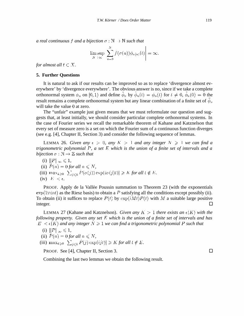
a real continuous f and a bijection � : N ! N such that

lim supN!1

��NXu=0

f(�(u))��(u)(t)

�� =1:

for almost all t 2 X .

5. Further Questions

It is natural to ask if our results can be improved so as to replace ‘divergence almost ev-erywhere’ by ‘divergence everywhere’. The obvious answer is no, since if we take a completeorthonormal system �n on [0; 1) and define ~�n by ~�n(t) = �n(t) for t 6= 0, ~�n(0) = 0 theresult remains a complete orthonormal system but any linear combination of a finite set of ~�nwill take the value 0 at zero.

The “unfair” example just given means that we must reformulate our question and sug-gests that, at least initially, we should consider particular complete orthonormal systems. Inthe case of Fourier series we recall the remarkable theorem of Kahane and Katznelson thatevery set of measure zero is a set on which the Fourier sum of a continuous function diverges(see e.g. [4], Chapter II, Section 3) and consider the following sequence of lemmas.

LEMMA 26. Given any � > 0, any K > 1 and any integer N > 1 we can find atrigonometric polynomial P , a set E which is the union of a finite set of intervals and abijection � : N ! Z such that

(i) jjP jj1 6 1,(ii) P (n) = 0 for all n 6 N ,

(iii) maxk>0 jP

j6k P (�(j)) exp(i�(j)t)j > K for all t =2 E.(iv) jEj < �.

PROOF. Apply de la Vallee Poussin summation to Theorem 23 (with the exponentialsexp(2�int) as the Riesz basis) to obtain a P satisfying all the conditions except possibly (ii).To obtain (ii) it suffices to replace P (t) by exp(iMt)P (t) with M a suitable large positiveinteger.

LEMMA 27 (Kahane and Katznelson). Given any K > 1 there exists an �(K) with thefollowing property. Given any set E which is the union of a finite set of intervals and hasjEj < �(K) and any integer N > 1 we can find a trigonometric polynomial P such that


(iii) maxk>0 jP

j6k P (j) exp(ijt)j > K for all t =2 E.

PROOF. See [4], Chapter II, Section 3.

Combining the last two lemmas we obtain the following result.


LEMMA 28. Given any � > 0, any K > 1 and any integer N > 1 we can find atrigonometric polynomial P and a bijection � : N ! Z such that


(iii) maxk>0 jP

j6k P (�(j)) exp(2�i�(j)t)j > K for all t 2 T.

It is now easy to prove the desired result.

THEOREM 29. We can find a continuous function f : T ! C with f(n) = 0 for n < 0

and a bijection � : N ! N such that

supk>0

j

Xj6k

f(�(j)) exp(2�ijt)j =1

for all t 2 T.

If instead of considering complex valued functions and the orthonormal system exp 2�int,we wish to consider real valued functions and the orthonormal system formed by sin 2�ntand cos 2�nt then we can replace the P of Lemma 28 by <P + =P and first sum thecos 2��(j)t terms and then the sin 2��(j)t terms. The existence of a continuous functionwhose rearranged Fourier series diverges everywhere was first proved by L. V. Taıkov [10]using Olevskiı’s theorem in a different way.

So far as I know the general question remains open. In particular we may ask the follow-ing question.

QUESTION 30. Consider the Haar system on [0; 1) ordered in some way. Does there exista continuous function f : [0; 1]! C and a bijection � : N ! N such that

supk>0

��kX

j=0

a�(j)��(j)(t)

�� =1

for all t 2 [0; 1)?

We remark that a similar proof to the one above (replacing the non-trivial lemma of Ka-hane and Katznelson by a trivial parallel lemma) gives the following.

LEMMA 31. Consider the Haar system on [0; 1) ordered in some way. There exists a realf 2 L2 and a bijection

� : N ! N

such that

supk>1

��kX

j=1

f(��(j))��(j)(t)

�� =1

for all t 2 [0; 1).


The method of proof applies to any ‘well behaved’ system (though the ‘unfair example’with which we began the section shows that it can not apply to all Riesz bases).

6. Hard summation

The reader with more practical interests will observe that striking as Kolmogorov’s the-orem and its generalisations may be, they do not answer the question in the case of any par-ticular rearrangement. Let us return to the question we started with but apply it to a generalothonormal system �1, �2, . . . . If f 2 L2 we consider

SÆ(t) =X

jf(n)j>Æ

f(n)�n(t)

where f(n) = hf; �ni is the usual Fourier coefficient for the given system. This method offorming a sum is called ‘hard summation’ and, as we said at the beginning of the talk, is avery natural one to use.

(The reader may well ask what ‘soft summation’ is. Here we consider something like

�ÆX

jf(n)j>Æ

f(n)�n(t) +X

Æ>jf(n)j>Æ=2

jf(n)j � Æ=2

Æ=2f(n)�n(t):

I suspect that the idea of soft summation derives from the use of Cesaro sums and similarfiltering techniques to improve the behaviour of Fourier sums. I also suspect that the anal-ogy is false since I know of no reason why soft summation should behave better than hardsummation. However, this is merely opinion, and like all opinion liable to be disproved byfact.)

In [5] I constructed the following example.

THEOREM 32. There exists a f 2 L2(T) such that

lim sup�!0+

��X

jf(u)j>�

f(u) exp 2�iut

�� =1:

for almost all t 2 T.

Later in [6] I showed that we could take f continuous.It therefore came as a great surprise to me to learn that Tao had proved the following

theorem

THEOREM 33. hard summation works for well behaved (rapidly decreasing) wavelets.

Still more surprising was the simple nature of his proof. In order to show how it works Iwill prove it in a special case where the argument is particularly clean.


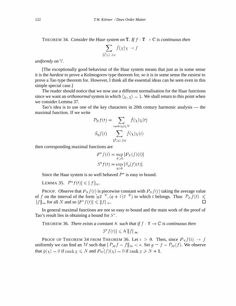
THEOREM 34. Consider the Haar system on T. If f : T ! C is continuous thenXjf(�)j>�

f(�)�! f

uniformly on T.

[The exceptionally good behaviour of the Haar system means that just as in some senseit is the hardest to prove a Kolmogorov type theorem for, so it is in some sense the easiest toprove a Tao type theorem for. However, I think all the essential ideas can be seen even in thissimple special case.]

The reader should notice that we now use a different normalisation for the Haar functionssince we want an orthonormal system in which h�; �i = 1. We shall return to this point whenwe consider Lemma 37.

Tao’s idea is to use one of the key characters in 20th century harmonic analysis — themaximal function. If we write

PNf(t) =X

rank(�)6N

f(�)�(t)

S�f(t) =X

jf(�)j>�

f(�)�(t)

then corresponding maximal functions are

P �f(t) = supN>0

jPN(f)(t)j

S�f(t) = sup�>0

jS�(f)(t)j:

Since the Haar system is so well behaved P � is easy to bound.

LEMMA 35. jP �f(t)j 6 kfk1.

PROOF. Observe that PNf(t) is piecewise constant with PNf(t) taking the average valueof f on the interval of the form [q2�N ; (q + 1)2�N) to which t belongs. Thus jPNf(t)j 6kfk1 for all N and so jP �f(t)j 6 kfk1.

In general maximal functions are not so easy to bound and the main work of the proof ofTao’s result lies in obtaining a bound for S�.

THEOREM 36. There exists a constant K such that if f : T ! C is continuous then

jS�f(t)j 6 Kkfk1:

PROOF OF THEOREM 34 FROM THEOREM 36. Let � > 0. Then, since PNf(t) ! funiformly we can find an M such that kPMf � fk1 < �. Set g = f � PM(f). We observethat g(�) = 0 if rank� 6 N and ^PM(f)(�) = 0 if rank� > N + 1.


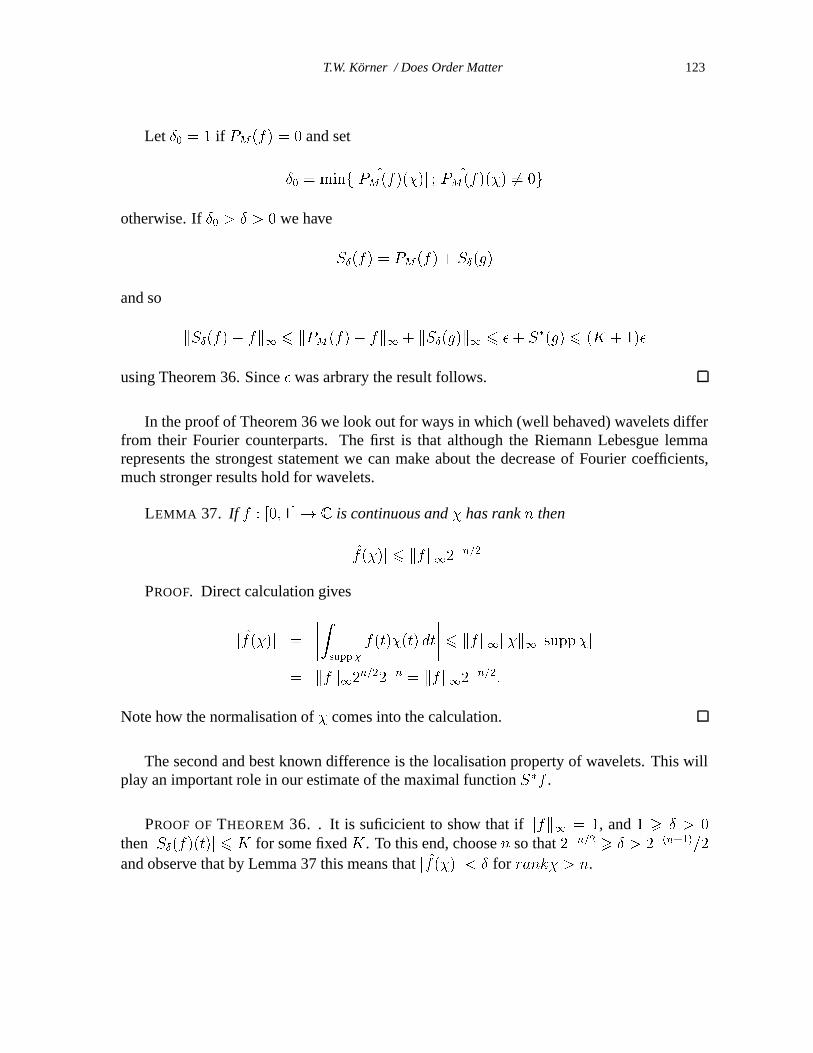
Let Æ0 = 1 if PM(f) = 0 and set

Æ0 = minfj ^PM(f)(�)j ; ^PM(f)(�) 6= 0g

otherwise. If Æ0 > Æ > 0 we have

SÆ(f) = PM(f) + SÆ(g)

and so

kSÆ(f)� fk1 6 kPM(f)� fk1 + kSÆ(g)k1 6 � + S�(g) 6 (K + 1)�

using Theorem 36. Since � was arbrary the result follows.

In the proof of Theorem 36 we look out for ways in which (well behaved) wavelets differfrom their Fourier counterparts. The first is that although the Riemann Lebesgue lemmarepresents the strongest statement we can make about the decrease of Fourier coefficients,much stronger results hold for wavelets.

LEMMA 37. If f : [0; 1]! C is continuous and � has rank n then

jf(�)j 6 kfk12�n=2

PROOF. Direct calculation gives

jf(�)j =

��Zsupp�

f(t)�(t) dt

�� 6 kfk1k�k1j supp�j

= kfk12n=22�n = kfk12�n=2:

Note how the normalisation of � comes into the calculation.

The second and best known difference is the localisation property of wavelets. This willplay an important role in our estimate of the maximal function S �f .

PROOF OF THEOREM 36. . It is suficicient to show that if kfk1 = 1, and 1 > Æ > 0

then jSÆ(f)(t)j 6 K for some fixed K. To this end, choose n so that 2�n=2 > Æ > 2�(n+1)=2

and observe that by Lemma 37 this means that jf(�)j < Æ for rank� > n.


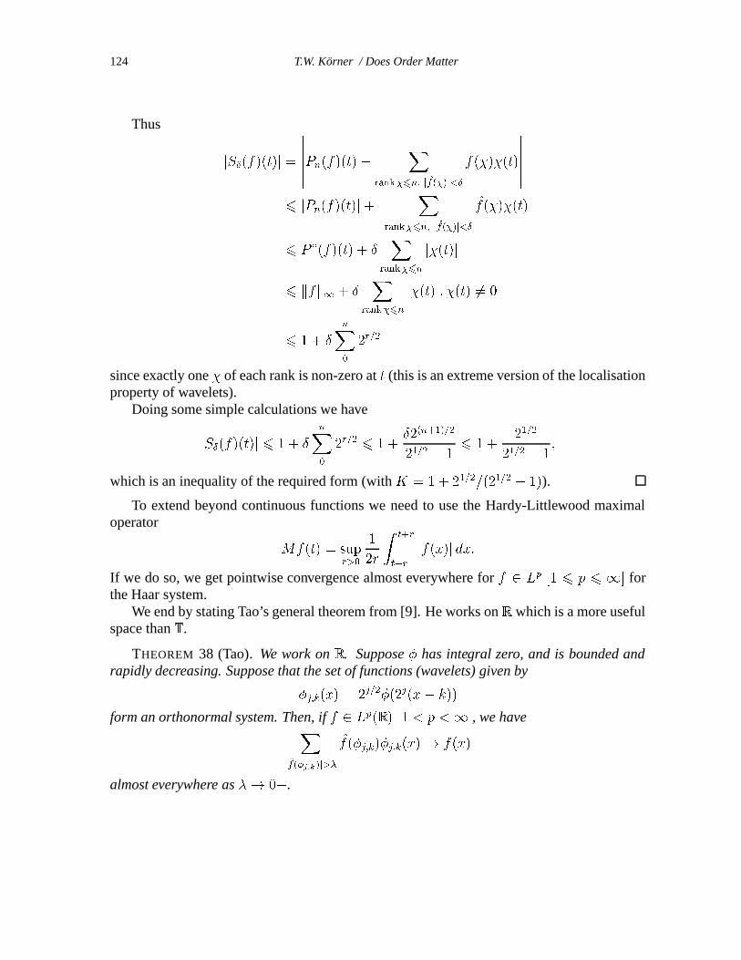
Thus

jSÆ(f)(t)j =

��Pn(f)(t)�X

rank�6n; jf(�)j<Æ

f(�)�(t)

��6 jPn(f)(t)j+ j

Xrank�6n; jf(�)j<Æ

f(�)�(t)j

6 P �(f)(t) + ÆX

rank�6n

j�(t)j

6 kfk1 + ÆX

rank�6n

j�(t)j; �(t) 6= 0

6 1 + ÆnX0

2r=2

since exactly one � of each rank is non-zero at t (this is an extreme version of the localisationproperty of wavelets).

Doing some simple calculations we have

jSÆ(f)(t)j 6 1 + ÆnX0

2r=2 6 1 +Æ2(n+1)=2

21=2 � 16 1 +

21=2

21=2 � 1;

which is an inequality of the required form (with K = 1 + 21=2=(21=2 � 1)).

To extend beyond continuous functions we need to use the Hardy-Littlewood maximaloperator

Mf(t) = supr>0

1

2r

Zt+r

t�r

jf(x)j dx:

If we do so, we get pointwise convergence almost everywhere for f 2 Lp [1 6 p 6 1] forthe Haar system.

We end by stating Tao’s general theorem from [9]. He works on R which is a more usefulspace than T.

THEOREM 38 (Tao). We work on R. Suppose � has integral zero, and is bounded andrapidly decreasing. Suppose that the set of functions (wavelets) given by

�j;k(x) = 2j=2�(2j(x� k))

form an orthonormal system. Then, if f 2 Lp(R) [1 < p <1], we haveXjf(�j;k)j>�

f(�j;k)�j;k(x)! f(x)

almost everywhere as �! 0+.


References

[1] N. Dunford and J. T. Schwartz, Linear Operators (Part I) (2nd Ed), Wiley, 1957.[2] W. Feller, An Introduction to Probability Theory and its Applications, (3rd Ed) Wiley, 1968.[3] P. R. Halmos Measure Theory, Van Nostrand, 1950.[4] Y. Katznelson An Introduction to Harmonic Analysis Wiley, 1968.[5] T. W. Korner, Divergence of decreasing rearranged Fourier series Ann. of Math. 144, no. 1, 167–180

(1996).[6] T. W. Korner Decreasing rearranged Fourier series J. Fourier Anal. Appl. 5 , no. 1, 1–19 (1999).[7] A. M. Olevskiı, Fourier Series with Respect to General Orthogonal Systems Springer 1975.[8] H. L. Royden, Real Analysis (2nd Ed), MacMillan, New York, 1968.[9] T. Tao On the almost everywhere convergence of wavelet summation methods Appl. Comput. Harmon.

Anal. 3, no. 4, 384–387 (1996).[10] L. V. Taıkov, The divergence of Fourier series of continuous functions with respect to a rearranged trigono-

metric system, Dokl. Akad. Nauk SSSR, 150, 262–265 (1963).

does order matter - nato-us.orgnato-us.org/analysis2000/papers/korner.pdf · does order matter t....

Documents