does non-farm sector employment reduce rural poverty and...
TRANSCRIPT
Economics Discussion Paper Series EDP-1226
Does non-farm sector employment reduce rural poverty and vulnerability? Evidence from
Vietnam and India
Katsushi S. Imai Raghav Gaiha Woojin Kang
Samuel Annim Ganesh Thapa
October 2013
Economics School of Social Sciences
The University of Manchester Manchester M13 9PL

Does non-farm sector employment reduce rural poverty and vulnerability?
Evidence from Vietnam and India
Katsushi S. Imai *
School of Social Sciences, University of Manchester, UK
Raghav Gaiha
Faculty of Management Studies, University of Delhi, India
Woojin Kang
Crawford School of Economics & Government, Australian National University, Australia
Samuel Annim
University of Cape Coast, Ghana & University of Central Lancashire, UK
Ganesh Thapa
International Fund for Agricultural Development, Rome, Italy
First Draft: 3
rd September 2012
First Draft: 8th October 2012
Abstract
The present study examines whether participation in the rural non-farm sector
employment or involvement in activity in rural non-farm economy (RNFE) has any poverty-reducing or vulnerability-reducing effect in Vietnam and India. To take account
of sample selection bias associated with RNFE, we have applied treatment-effects
model, a variant of Heckman sample selection model. It is found that log per capita
consumption or log mean per capita expenditure (MPCE) significantly increased as a result of access to RNFE in 2002 and 2004 for Vietnam and in 1993-4 for India. This is
consistent with poverty reducing role of accessing RNFE. However, in more recent
years, this consumption poverty reducing effect disappeared. That is, it was no longer statistically significant in 2006 for Vietnam and MPCE slightly reduced due to access to
RNFE in 2004-5 for India. Access to RNFE significantly reduces vulnerability in India,
implying that diversification of household activities into non-farm sector would reduce such risks. However, in Vietnam, RNFE increased vulnerability in 2002, but the effect
vanished in 2004 and 2006.
Key Words: Poverty, Vulnerability, Non-farm sector, Treatment Effects Model, Vietnam, India
JEL Codes: C21, C31, I32, O15
Contact Address
Katsushi S. Imai (Dr) Economics, School of Social Sciences, University of Manchester,
Arthur Lewis Building, Oxford Road, Manchester M13 9PL, UK; Telephone:
+44-(0)161-275-4827, Fax: +44-(0)161-275-4812 Email: [email protected].
Acknowledgements
This project is has been funded by IFAD. We acknowledge valuable comments and advice
from Armando Barrientos, Takahiro Sato, Md. Azam, and Md. Faruq Hassan. The views
expressed are, however, those of the authors’ and do not necessarily represent those of the
organisations to which they are affiliated.
2
Does non-farm sector employment reduce poverty and vulnerability?
Evidence from Vietnam and India
1. Introduction
Across the developing world, it is well recognized that rural economies are not purely
agricultural and farm households earn an increasing share of their income from non-farm
activities. Traditionally, rural non-farm economy (RNFE) was considered to be a
low-productivity sector diminishing over time where agricultural households simply
supplement their income. But, since the late 1990s, its role in economic growth and poverty
reduction began to be increasingly recognised given the increasing share of RNFE across
developing countries (e.g. Lanjouw and Lanjouw, 2001, Haggblade, et al., 2010). The share
of income from RNFE in total rural income varies - from 34% in Africa, to 47% in Latin
America and 51% in Asia, but it is recognised that RNFE is becoming increasingly important
in terms of its share and growth as well as potential roles in poverty reduction in Asia,
particularly in emerging countries, such as China and India. Although most of the low and
middle-income Asian countries traditionally relied on agriculture, they have undergone
structural changes in recent years, due to industrialisation and globalisation as well as
commercialisation of agriculture.
Within Asia, the share of income from RNFE varies from over 70% for the Philippines
and Sri Lanka to below 40% for China, India and Nepal. With constraints on farm expansion
and continuing growth of rural population, greater attention is thus being given to non-farm
activities. Policy interest in RNFE arises not just because of its significance in generating
incomes, but also because of its increasing importance in creating employment, especially for
rural women and the poor.
Among Asian countries, the present study focuses on two countries – Vietnam and
India, both of which experienced spectacular economic growth rate as well as poverty

3
reduction in recent years. These two countries are characterised by high average GDP per
capita growth rate in 1990-2010 (Vietnam 5.8%; India 4.9%) and a decreasing share of
agricultural value added in GDP (Vietnam 39% to 20%; India 29% to 16%). Poverty indices
have declined during this period, but there is a variation in the speed of poverty reduction.
While Vietnam experienced a faster poverty reduction in terms of headcount ratio based on
US$1.25 (64% in 1993 to 21% in 2006, further down to 13% in 2008), the speed of poverty
reduction has been relatively slow in India (49% in 1994 to 42% in 2005). As shown by Imai
et al. (2012a, b) and Gaiha et al. (2012 a, b), the speed of improvement in nutritional
indicators has been slow in India in recent years despite the country's economic growth.
There is a need for investigating the reasons for diverse progress in income and non-income
poverty focusing on household's livelihood strategies, including the choice of farm and
non-farm employment. The present study will aim to provide insights into different pace of
poverty reduction and vulnerability in these two countries.
The main hypothesis we examine is whether access to RNFE reduces poverty in rural
areas in Vietnam and India. We focus only on rural areas because rural economy is distinct
from urban economy in its structure and rural poverty is still predominant in these countries.
We will use Vietnam Household Living Standards Survey (VHLSS) in 2002, 2004 and 2006
for Vietnam as well as National Sample Survey Data in 1993-4 and 2004-5 for India. Given
the sample selection bias associated with access to RNFE or non-farm sector employment
and the data structure where only large cross-sectional data are available and the panel data
are not available1, we will apply treatment effects model, a variant of Heckman two-step
sample selection model (Heckman, 1979).
1 It is possible to construct a panel based on the intersections of different rounds of household
cross-sectional data of VHLSS in Vietnam, but attrition bias is serious. See Imai et al. (2011) for
details.

4
While the farm or agricultural sector has played a central role in these countries, the
share of non-farm activities has increased significantly in recent years. However, detailed
empirical studies estimating the direct and/or indirect effects of rural non-farm income or
employment on poverty remain limited and the present study seeks to fill this gap. The rest of
the paper is organised as follows. The next section reviews extant studies on the effects of
non-farm sector on poverty in Vietnam and India. Section 3 briefly summarises the data sets
we will use. Sections 4 and 5 discuss the specification of econometric models and results,
respectively. Concluding observations are offered in the final section.
2. The Literature
While the farm or agricultural sector has played a central role in Vietnam and India, the share
of non-farm has increased significantly in recent years. However, formal empirical studies to
estimate the direct and/or indirect effects of income or employment in non-farm sector
employment on poverty are still few. On the direct effects, van de Walle and Cratty (2004)
using VLSS data on Vietnam in 1993 and 1998 found significant effects of non-farm
employment in reducing poverty. While van de Walle and Cratty (2004) claim that they
consider the endogeneity of non-farm sector in reducing poverty, they simply estimated the
share of hours worked in non-farm sector in total (or the probability of participating in
non-farm sector) and poverty separately and compared the signs and statistical significance
of coefficient estimates of explanatory variables without taking account of simultaneity. Thus
their results are only suggestive of different covariates of non-farm employment and poverty.
Informal evidence from India and Bangladesh suggests that indirect effects also matter, for
example, the labour market tightening, or expansion of casual non-farm employment is
strongly correlated with growth in agricultural wages. While building upon van de Walle and

5
Cratty (2004), our proposed research applies improved methodologies to take account of the
endogeneity issues to more comprehensive and recent data sets.
RNFE would be potentially important for breaking the poverty traps through various
routes - such as lack of education and/or nutrition. For example, people who are educated at
secondary school or higher are likely to have a higher probability of finding a job in rural
non-farm sector (e.g. in trading, manufacturing office works) and their children tend to be
more educated, which causes a 'virtuous' circle (e.g. Knight et al., 2009, 10). However, those
who are not educated tend to be trapped in a 'vicious' circle. Likewise, undernourished people
tend to be trapped in poverty as low nutritional levels imply low efficiency and high
probability of being unemployed as predicted by the efficiency-wage hypothesis (e.g. Bliss
and Stern, 1978, Dasgupta and Ray, 1986, 87). The poverty-nutrition hypotheses have been
recently examined by Jha et al (2009) and Imai et al. (2012a) in the context of rural India.
Reardon et al. (2000) also emphasises the barriers faced by poor households that prevent
them from investing in non-farm assets, suggesting the existence of the poverty trap. That is,
it is not an automatic process for poor agricultural households to enter into the non-farm
sector. Unlike agricultural jobs, rural non-farm employment tends to be less physically
intensive and requires lower calories, as the activity intensity determines the nutritional status
in rural India Imai et al. (2012b). Since RNFE tend to better promote food security to the
poor than farm employment (Owsu et al., 2011), the former has the potential to break the
poverty trap.
3. Data
Vietnamese Data
We will use Vietnam Household Living Standards Surveys (VHLSS) 2002, 2004, and 2006.
The VHLSSs were initially implemented in 2002 to collect detailed household and commune
level data. These are multi-topic household surveys with nationally representative household
6
samples. They commonly cover a wide range of issues, including household composition and
characteristics (e.g. education and health); detailed record on expenditure for both food and
non-food items, health and education; employment and labour force participation (e.g.
duration of employment and the precise categories of occupations); income by sources (e.g.
salary/wage, payment in cash and in kind, farm and non-farm production etc.); housing,
ownership of assets and durable goods; and participation of households in anti-poverty
programs. Commune level surveys collect data on demography, economic conditions,
agricultural production, and non-farm employment, local infrastructure, public services such
as education and health facilities.
Indian Data2
The NSS, set up by the Government of India in 1950, is a multi-subject integrated sample
survey conducted all over India in the form of successive rounds relating to various aspects
of social, economic, demographic, industrial and agricultural statistics. We use the data in the
‘Household Consumer Expenditure’ schedule, quinquennial surveys in the 50th round,
1993–94 and in the 61st round, 2004-05.
3 These form repeated cross-sectional data sets, each
of which contains a large number of households across India.4 The consumption schedule
contains a variety of information related to mean per capita expenditure (MPCE),
disaggregated expenditure over many items together with basic socio economic
characteristics of the household (e.g., sex, age, religion, caste, and land-holding). To derive
wages at the level of NSS region, we supplement the consumption schedule by Employment
2 This sub-section draws upon Imai (2011).
3 We are not using 55
th round in 1999-2000 as the consumption data in 55
th round are not comparable
with those in 50th or 61
st round because of the change in recall periods. The consumption data are
comparable between 50th
round and 61st round.
4 After dropping the households with missing observations in one of the explanatory variables, the
number of households used for the estimation is 69206 and 78999 respectively for 50th and 61
st
rounds, respectively.
7
and Unemployment schedule because the consumption survey and the employment survey
collect data on different households and can be linked only at the aggregate level (e.g. NSS
region level).5
4. Methodologies
(1) Treatment Effects Model
To estimate the effect of non-farm sector employment on poverty and vulnerability, we
employ a version of treatment effects model. The main idea of treatment effects is to estimate
poverty defined by household consumption per capita for two different regimes (de Janvry et
al., 2005) - households participating only in the farm labour market and those participating in
both farm and non-farm labour markets. It is a version of the Heckman sample selection
model (Heckman, 1979), which estimates the effect of an endogenous binary treatment. This
would enable us to take account of the sample selection bias associated with access to
non-farm sector. In the first stage, access to non-farm sector is estimated by the probit
model.6 In the second, we estimate log of household consumption or vulnerability measure
after controlling for the inverse Mills ratio which reflects the degree of sample selection bias.
The merit of treatment effects model is that sample selection bias is explicitly
estimated by using the results of probit model. However, the weak aspects include (i) strong
assumptions are imposed on distributions of the error terms in the first and second stages; (ii)
the results are sensitive to choice of the explanatory variables and instruments; and (iii) valid
instruments are rarely found in non-experimental data and if the instruments are invalid, the
results will depend on the distributional assumptions.
5 Definitions of the variables of VHLSS and NSS data are provided in Appendix 1.
6 For Vietnam we estimate access to non-farm sector by the probit model at individual levels and
then estimate poverty (or log per capita real consumption or vulnerability) in the second. On the other
hand, only household-level estimations are possible for India because of the data constraint. That is, we run the probit model at household levels for whether any household members have access to
non-farm sector and then estimate the poverty equation in the second stage.

8
The selection mechanism by the probit model for accessing rural non-farm economy
(RNFE) can be more explicitly specified as (e.g., Greene, 2003):
iii uXD
* (1)
and 01**
iii XDifD
otherwiseDi 0*
where )(1Pr iii XXD
)(10Pr iii XXD
*D is a latent variable. In our case, D takes the value 1 if an ith individual has access to
RNFE (non-farm employment or non-farm activity) and 0 otherwise and X is a vector of
individual, household and regional characteristics and other determinants at commune or
community levels.7 denotes the standard normal cumulative distribution function.
Since available variables are different for Vietnam and India, we assume different
specifications (or the choice of explanatory variables) for individual access to RNFE for iX .
Vietnam:
),,,,,(*
RLHEMWDD hhiiiii (1)’
iW : Real average hourly wage rate for the ith
individual.
We assume here that the labour productivity proxied by average hourly wage rate is an
important determinant of RNFE. That is, only high productivity worker with higher
agricultural wages rate can participate in RNFE as an analogy of theory of workfare where
only high productivity workers can participate in workfare scheme or higher waged workers
7 The estimation for (1) is made at individual levels, but we omit subscript for simplicity.

9
can afford exercising the ‘real option’ of switching from the agriculture labour marker to
workfare or the non-farm labour market given the switching costs (Scandizzo et al., 2009).8
iM : Whether the ith individual is male.
iE : A set of dummy variables of educational attainment of the individual (whether he or she
has no education; whether completed primary education; whether completed lower secondary
education; whether completed upper secondary education; whether completed technical
education; whether completed higher education).
hH : Household compositions/ characteristics (household size; the share of female members;
dependency burden (the share of household members below 15 years or above 65 years;
whether a household belongs to ethnic majority) for the hth
household.
hL : Size of land (in hectare) owned by the household and its square for the hth
household.
R : A set of regional dummy variables (whether a household is located in red river delta
region; northeast region; northwest region; north central coast region; south central coast
region; central highlands region; north east south region; Mekong river delta region; central
coast region; low mountains; and high mountains).
India:
Because of data limitations, a different set of explanatory variables is chosen as determinants
of accessing RNFE.
),,,,,(*
RBLEHWDD hhhhhh (1)’’
iW : Wage rate estimated using employment data and aggregated for NSS region.9
8 Two issues should be discussed regarding the effects of wage rates on participation in RNFE. First,
access to non-farm sector employment is likely to have an indirect effect of reducing consumption
poverty of an agricultural household through increased agricultural wage rates. This would require the disaggregated non-farm and farm wages data (possibly over time), which neither VHLSS nor NSS
data have. Second, related to the first point, the wage rate is endogenous. Due to the lack of
instrument, we use the raw wage rate for VHLSS. While acknowledging the possibility that the potential endogeneity could potentially bias the coefficient estimates, we estimated the same model
without wage rate, but the final results did not change. For NSS data, we use the estimated wage rate
aggregated at NSS region level.

10
hH : A set of variables indicating household composition, such as whether a household is
headed by a female member, number of adult male or female members, dependency burden:
the share of household members under 15 years old or over 60 years old).10
hE : A set of variables on the highest level of educational attainment of household members
(e.g. whether completed primary school, secondary school, or higher education).
hL : Owned land as a measure of household wealth.
hB : Social backwardness of the household in terms of (i) whether a household belongs to
Scheduled Castes (SCs) and (ii) whether it belongs to Scheduled Tribes (STs).
R : A vector of state dummy variables.
The linear outcome regression model in the second stage is specified below to
examine the determinants of poverty – as proxied by household consumption (log of MPCE
for the Indian NSS data and log of per capita real household consumption for the Vietnamese
VHLSS data) or vulnerability derived by Chaudhuri’s (2003) method which captures the
probability of household falling into poverty in the next period.11
It is noted here that
non-farm labour marker participation is estimated at individual level in the first stage of the
treatment effects model, while poverty is estimated at household level (proxied by log per
capita household consumption or household vulnerability) in the second stage. Two reasons
justify this: one is limited individual earning data, and, the second is likely pooling of
individual earnings. We use log household consumption and vulnerability measure as a
measure of poverty because treatment effects model assumes that the dependent variable in
the second stage is continuous and the standard binary measure of poverty (0 or 1) cannot be
9 The results for wage equations (based on NSS50-10 and NSS61-10) are given in Appendix 2.
However, we have used wage rates only for NSS50. For NSS61, we have used the regional price
because aggregate wage rate is automatically dropped due to the collinearity problem. 10
Female headedness was dropped in all the regressions based on NSS50, because it consistently
shows a counter-intuitive sign. 11
The methodology will be discussed in the next subsection.

11
used. Moreover, as suggested by previous literature, households in India and Vietnam tend to
be vulnerable to shocks (e.g. Imai et al, 2011; Gaiha and Imai, 2009). We denote household
poverty – either log per capita household consumption or vulnerability - asiW .
iihi DZW (2)
12
,u ~ bivariate normal ,,1,0,0 .
where is the average net effect of access to RNFE. In case log per capita household
consumption is estimated, the positive estimate for implies that accessing RNFE increases
consumption and thus decreases poverty. In the case of vulnerability, the negative estimate
for implies that RNFE decreases vulnerability.
Here hZ is a vector of determinants ofW . For Vietnam this is estimated by:
),,,( RLHIZZ hhhhh (2)’
where hI is a vector of household head characteristics (educational attainment – defined the
same way as in the equation (1); sex; married). hH (a vector of household
characteristics), hL (land), and R (a vector of regional characteristics) are same as those for
equation (1)’.
For India, equation (2) is estimated by the same set of explanatory variables as in
equation (1)’’ exceptW .
),,,,( RBLEHZZ hhhhhh (2)’’
Using a formula for the joint density of bivariate normally distributed variables, the
expected poverty for those with access to RNFE is written as:
i
i
i
iiiii
X
XZ
DEZDWE
11
(3)
12
For India equation (2) is hhhh DZW as the estimation is done at household level.
12
where is the standard normal density function. The ratio of and is called the inverse
Mill’s ratio.
Expected poverty (or undernutrition or vulnerability) for non-participants is:
i
i
i
iiiii
X
XZ
DEZDWE
1
00
(4)
The expected effect of poverty reduction associated with RNFE is computed as
(Greene, 2003, 787-789):
ii
i
iiiiXX
XDWEDWE
101
(5)
If is positive (negative), the coefficient estimate of using OLS is biased upward
(downward) and the sample selection term will correct this. Since is positive, the sign
and significance of the estimate of (usually denoted as ) will show whether there
exists any selection bias. To estimate the parameters of this model, the likelihood function
given by Maddala (1983, 122) is used where the bivariate normal function is reduced to the
univariate function and the correlation coefficient . The predicted values of (3) and (4) are
derived and compared by the standard t test to examine whether the average treatment effect
or poverty reducing effect is significant.
The results of treatment effects model will have to be interpreted with caution
because the results are sensitive to the specification of the model or the selection of
explanatory variables and/or the instrument. Also important are the distributional
assumptions of the model. Despite these limitations, the model is one of the few available
methods to control for sample selection bias and capable of yielding insights into whether
access to RNFE leads to poverty reduction.

13
(2) Vulnerability Measure
It would be ideal to use panel data to derive household’s vulnerability measures, but, in its
absence, we can derive a measure of ‘Vulnerability as Expected Poverty’ (VEP), an ex ante
measure, based on Chaudhuri (2003) and Chaudhuri, Jalan and Suryahadi (2002) who
applied it to a large cross-section of households in Indonesia13
and defined vulnerability as
the probability that a household will fall into poverty in the future after controlling for the
observable household characteristics. Accordingly, it takes the value from 0 to 1, and the
higher the value of vulnerability measure, the higher is the probability of a household falling
into poverty in the next period. Imai et al. (2011) derived and analysed Chaudhuri’s
vulnerability measure using the VHLSS data for Vietnam, and Imai (2011) derived it using
the Indian NSS data. We will use these cross-sectional vulnerability measures subject to the
caveat of estimating vulnerability from a single cross-section that cannot captures the effect
of aggregate shocks affecting all the households in the sample area. The details of derivation
of Chaudhuri’s vulnerability measure is found on Appendix 3. Imai et al. (2011) and Imai
(2011) provide a full set of results of vulnerability for Vietnam and India.
4. Econometric Results
This section summarises the results of treatment effects model which are applied to estimate
the effects of participation in RNFE (Rural Non-farm Economy) or non-farm sector
employment. Vulnerability estimates based on VHLSS and NSS data are reported in Imai et
al. (2011) and Imai (2011) and we highlight only the results of treatment-effects model.
Table 1 gives the results of treatment effects model applied to VHLSS data in 2002,
2004 and 2006. For each year, two different proxies for poverty have been tried as a
13 See a summary by Hoddinott and Quisumbing (2003a, b) of methodological issues in
measuring vulnerability.

14
dependent variable - log of per capita consumption and vulnerability. The second panel
reports the results of the first stage probit model for whether an individual participates in the
non-farm sector labour market and the first panel gives the results for OLS whereby log per
capita consumption or vulnerability is estimated.
The second panel of Table 1 suggests that individual and household characteristics (e.g.
individual productivity, individual education attainment, household composition, location)
affect the probability of an individual participating in the non-farm sector labour market. For
example, real hourly wage rate significantly increases the probability of participating in
RNFE. Other variables show more or less expected results (e.g. lower educational attainment
tends to decrease the probability of participating in RNFE (except 2006); belonging to ethnic
majorities increase the probability (except 2006); locations affect the probability). or
in the equation (3) is statistically significant only in the case of vulnerability in 2002. A
relatively high estimate of (0.233) implies the high correlation between the first stage
and the second stage equations in case of log per capita consumption in 2004 where is
not significant, but with a relatively high z value of 1.57. Use of treatment effects model is
justified in these cases. Sample selection term is not significant in other cases.
The first panel of Table 1 shows the results of determinants of per capita consumption
and vulnerability for 2002, 4 and 6. For example, size of household significantly decreases
consumption in all the years and significantly decreases vulnerability in 2004 and 6. A
household headed by an older head tends to have higher per capita consumption and lower
vulnerability with non-linear effects. Higher dependency burden is associated with lower
consumption and higher vulnerability. Education and location are important determinants of
both consumption and vulnerability.
At the bottom of the table, ATE (average treatment effects) as well as ANF (average
net effects) associated with the individual participation in RNFE are reported. The former is

15
the difference of the expected outcome for participants in RNFE and for non-participants
after controlling for sample selection (as in equation (5), sum of ANF and sample selection
term). The latter is the net effect which is purely associated with access to RNFE without
controlling for sample selection. In order to evaluate the effect of access to RNFE on poverty
after taking account of sample selection, we need to base our discussion on the former, not
the latter (Imai, 2011).
In 2002, per capita consumption is significantly higher by 1.3% for participants in the
non-farm labour market14
than for non-participants after taking account of sample selection,
which is consistent with the poverty reducing role of RNFE. Average net effect is 2.9% and
significant (Column 1 of Table 1). In the same year, however, whilst RNFE significantly
reduces vulnerability by 2.3% as a net effect, it increases the vulnerability by 0.16% on
average after taking account of sample selection (Column 1). Admittedly, this is not large. In
2004, per capita consumption is significantly higher by 3.8% for non-farm labour market
participants than for non-participants after controlling for sample selection, while
vulnerability is also higher for non-farm labour market participants by 0.9%. In 2006, there
are no statistically significant effects of access to RNFE either for consumption or
vulnerability. However, these effects were weak or weaker in 2006.
14
It is noted that those self-employed are excluded from the sample.
16
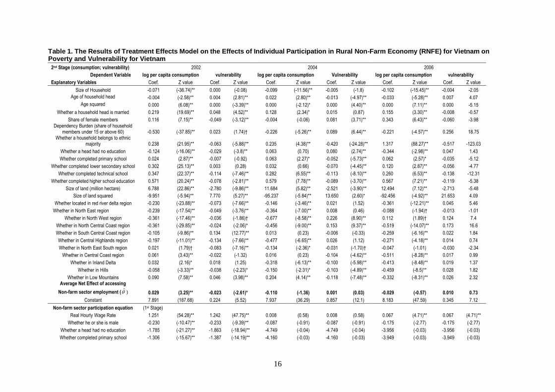
Table 1. The Results of Treatment Effects Model on the Effects of Individual Participation in Rural Non-Farm Economy (RNFE) for Vietnam on Poverty and Vulnerability for Vietnam
2nd Stage (consumption; vulnerability) 2002 2004 2006
Dependent Variable log per capita consumption vulnerability log per capita consumption Vulnerability log per capita consumption vulnerability
Explanatory Variables Coef. Z value Coef. Z value Coef. Z value Coef. Z value Coef. Z value Coef. Z value
Size of Household -0.071 (-36.74)** 0.000 (-0.08) -0.099 (-11.56)** -0.005 (-1.8) -0.102 (-15.45)** -0.004 -2.05
Age of household head -0.004 (-2.58)** 0.004 (2.81)** 0.022 (2.80)** -0.013 (-4.97)** -0.033 (-5.28)** 0.007 4.07
Age squared 0.000 (6.08)** 0.000 (-3.39)** 0.000 (-2.12)* 0.000 (4.40)** 0.000 (7.11)** 0.000 -5.15
Whether a household head is married 0.219 (19.69)** 0.048 (4.52)** 0.128 (2.34)* 0.015 (0.87) 0.155 (3.30)** -0.008 -0.57
Share of female members 0.116 (7.15)** -0.049 (-3.12)** -0.004 (-0.06) 0.081 (3.71)** 0.343 (6.43)** -0.060 -3.98
Dependency Burden (share of household members under 15 or above 60) -0.530 (-37.85)** 0.023 (1.74)† -0.226 (-5.26)** 0.089 (6.44)** -0.221 (-4.57)** 0.256 18.75
Whether a household belongs to ethnic majority 0.238 (21.95)** -0.063 (-5.88)** 0.235 (4.38)** -0.420 (-24.28)** 1.317 (88.27)** -0.517 -123.03
Whether a head had no education -0.124 (-16.06)** -0.029 (-3.8)** 0.063 (0.70) 0.080 (2.74)** -0.344 (-2.98)** 0.047 1.43
Whether completed primary school 0.024 (2.87)** -0.007 (-0.92) 0.063 (2.27)* -0.052 (-5.73)** 0.062 (2.57)* -0.035 -5.12
Whether completed lower secondary school 0.302 (25.13)** 0.003 (0.28) 0.032 (0.66) -0.070 (-4.45)** 0.120 (2.87)** -0.056 -4.77
Whether completed technical school 0.347 (22.37)** -0.114 (-7.46)** 0.282 (6.55)** -0.113 (-8.10)** 0.260 (6.53)** -0.138 -12.31
Whether completed higher school education 0.571 (20.24)** -0.078 (-2.81)** 0.579 (7.78)** -0.089 (-3.70)** 0.567 (7.21)** -0.119 -5.38
Size of land (million hectare) 6.788 (22.86)** -2.780 (-9.86)** 11.684 (5.82)** -2.521 (-3.90)** 12.494 (7.12)** -2.713 -5.48
Size of land squared -9.951 (-5.94)** 7.770 (5.27)** -95.237 (-5.84)** 13.650 (2.60)* -92.456 (-4.92)** 21.653 4.09
Whether located in red river delta region -0.230 (-23.88)** -0.073 (-7.66)** -0.146 (-3.46)** 0.021 (1.52) -0.361 (-12.21)** 0.045 5.46
Whether in North East region -0.239 (-17.54)** -0.049 (-3.76)** -0.364 (-7.00)** 0.008 (0.46) -0.088 (-1.94)† -0.013 -1.01
Whether in North West region -0.361 (-17.46)** -0.036 (-1.86)† -0.677 (-8.58)** 0.226 (8.90)** 0.112 (1.89)† 0.124 7.4
Whether in North Central Coast region -0.361 (-29.85)** -0.024 (-2.06)* -0.456 (-9.00)** 0.153 (9.37)** -0.519 (-14.07)** 0.173 16.6
Whether in South Central Coast region -0.105 (-9.86)** 0.134 (12.77)** 0.013 (0.23) -0.006 (-0.33) -0.259 (-6.16)** 0.022 1.84
Whether in Central Highlands region -0.197 (-11.01)** -0.134 (-7.66)** -0.477 (-6.65)** 0.026 (1.12) -0.271 (-4.18)** 0.014 0.74
Whether in North East South region 0.021 (1.79)† -0.083 (-7.16)** -0.134 (-2.36)* -0.031 (-1.70)† -0.047 (-1.01) -0.030 -2.34
Whether in Central Coast region 0.061 (3.43)** -0.022 (-1.32) 0.016 (0.23) -0.104 (-4.62)** -0.511 (-8.28)** 0.017 0.99
Whether in Inland Delta 0.032 (2.16)* 0.018 (1.25) -0.318 (-6.13)** -0.100 (-5.98)** -0.413 (-8.48)** 0.019 1.37
Whether in Hills -0.058 (-3.33)** -0.038 (-2.23)* -0.150 (-2.31)* -0.103 (-4.89)** -0.459 (-8.5)** 0.028 1.82
Whether in Low Mountains 0.090 (7.58)** 0.046 (3.98)** 0.204 (4.14)** -0.118 (-7.48)** -0.332 (-8.31)** 0.026 2.32 Average Net Effect of accessing
Non-farm sector employment ( ) 0.029 (3.25)** -0.023 (-2.61)* -0.110 (-1.36) 0.001 (0.03) -0.029 (-0.57) 0.010 0.73
Constant 7.891 (187.68) 0.224 (5.52) 7.937 (36.29) 0.857 (12.1) 8.183 (47.59) 0.345 7.12
Non-farm sector participation equation (1st Stage)
Real Hourly Wage Rate 1.251 (54.28)** 1.242 (47.75)** 0.008 (0.58) 0.008 (0.58) 0.067 (4.71)** 0.067 (4.71)**
Whether he or she is male -0.230 (-10.47)** -0.233 (-9.39)** -0.087 (-0.91) -0.087 (-0.91) -0.175 (-2.77) -0.175 (-2.77)
Whether a head had no education -1.785 (-21.27)** -1.863 (-18.94)** -4.749 (-0.04) -4.749 (-0.04) -3.956 (-0.03) -3.956 (-0.03)
Whether completed primary school -1.306 (-15.67)** -1.387 (-14.19)** -4.160 (-0.03) -4.160 (-0.03) -3.949 (-0.03) -3.949 (-0.03)

17
Whether completed lower secondary school -0.949 (-11.33)** -1.012 (-10.31)** -3.709 (-0.03) -3.709 (-0.03) -3.515 (-0.03) -3.515 (-0.03)
Whether completed upper secondary school -0.598 (-6.75)** -0.693 (-6.69)** -3.402 (-0.03) -3.404 (-0.03) -3.123 (-0.03) -3.123 (-0.03)
Whether completed technical school -0.092 (-0.93) -0.195 (-1.71)** -3.167 (-0.02) -3.166 (-0.02) -2.853 (-0.03) -2.853 (-0.03)
Whether completed higher school education -
- -2.600 (-0.02) -2.600 (-0.02) -3.055 (-0.03) -3.055 (-0.03)
Size of household -0.009 (-1.34) -0.006 (-0.81) -0.016 (-0.34) -0.015 (-0.33) -0.012 (-0.27) -0.012 (-0.27)
Share of female members -0.036 (-0.64) -0.050 (-0.77) 0.985 (2.65)* 0.984 (2.65)* -0.134 (-0.37) -0.134 (-0.37)
Dependency Burden -0.111 (-2.39)* -0.125 (-2.37)* 0.191 (0.79) 0.189 (0.79) 0.014 (0.05) 0.014 (0.05)
Whether belongs to Majorities 0.127 (3.17)** 0.113 (2.45)* 0.048 (0.14) 0.048 (0.14) 0.017 (0.19) 0.017 (0.19)
Whether in Red River Delta 0.004 (0.11) -0.037 (-0.96) 0.058 (0.28) 0.058 (0.28) -0.106 (-0.64) -0.106 (-0.64)
Whether in North East region 0.045 (0.9) 0.026 (0.47) 0.643 (2.15)* 0.644 (2.15)* 0.377 (1.14) 0.377 (1.14)
Whether in North West region 0.210 (2.69)** 0.133 (1.56) 0.267 (0.55) 0.267 (0.55) -0.236 (-0.58) -0.236 (-0.58)
Whether in North Central Coast region 0.017 (0.4) 0.008 (0.16) 0.086 (0.31) 0.086 (0.31) 0.283 (1.08) 0.283 (1.08)
Whether in South Central Coastal region -0.012 (-0.3) -0.036 (-0.8) 0.517 (1.61) 0.517 (1.61) 0.279 (0.92) 0.279 (0.92)
Whether in Central Highlands region 0.069 (1.03) 0.015 (0.2) 0.163 (0.37) 0.163 (0.37) -0.186 (-0.36) -0.186 (-0.36)
Whether North East South region 0.083 (1.92)† 0.053 (1.03) 0.326 (1.03) 0.320 (1.01) 0.346 (0.96) 0.346 (0.96)
Size of land (million hectare) 0.407 (0.36) 0.028 (0.02) 29.663 (2.03)* 29.492 (2.02)* -0.634 (-0.05) -0.634 (-0.05)
Size of land squared -4.980 (-0.75) -4.335 (-0.63) -227.254 (-2.28)* -226.173 (-2.27)* -34.848 (-0.30) -34.848 (-0.30)
Whether Central Coast Region -0.039 (-0.59) -0.066 (-0.89) -0.330 (-0.80) -0.329 (-0.80) -0.133 (-0.25) -0.133 (-0.25)
Whether Inland Delta Region 0.039 (0.69) 0.018 (0.28) -0.167 (-0.50) -0.168 (-0.50) -0.438 (-1.05) -0.438 (-1.05)
Whether in Hills -0.028 (-0.43) -0.073 (-0.98) -0.503 (-1.27) -0.510 (-1.29) -0.523 (-1.16) -0.523 (-1.16)
Whether in Low Mountains 0.020 (0.45) 0.003 (0.06) -0.220 (-0.68) -0.220 (-0.68) -0.546 (-1.59) -0.546 (-1.59)
Constant 0.538 (4.68) 0.673 (5.04) 4.338 (0.03) 4.339 (0.03) 5.116 (0.04) 5.116 (0.04)
-0.009 (-1.27) 0.0124 (1.92)† 0.072 (1.57) 0.004 (0.26) 0.021 0.74 -0.004 -0.55
-0.021
0.0365 0.233
0.038 0.082
-0.062
No. of Observations 20848 16031 1427 1426 3136 3136
Wald Chi2(44) 12604** 1010** 1275** 3030** 24293** 37998**
Average Treatment Effect (ATE)
Variable log per capita consumption Vulnerability log per capita consumption Vulnerability log per capita consumption vulnerability
Treat With RNFE 7.789 0.216 8.129 0.058 8.207 0.230
Control Without RNFE 7.776 0.215 8.092 0.049 8.193 0.229
ATE (
ii
i
XX
X
1)
0.013 0.0016 0.038 0.009 0.014 0.001
t value ( ) (4.17)** (1.99)** (3.45)** (1.57) (0.78) (0.22)
Does RNFE Reduce Poverty (or Vulnerability) Significantly?
(based on ANF)
0.029
(3.25)**
-0.023
(2.61)*
-0.110
(1.36)
0.001
(0.03)
-0.029
(0.57)
0.010
(0.73)
Does RNFE Reduce Poverty (or Vulnerability) Significantly? (based on ATE) YES NO YES NO NO NO

18
In sum, we confirm that RNFE reduced consumption poverty in 2002 and 2004, but at
the same time, consumption vulnerability (as a probability of falling into consumption
poverty) slightly increased in these years. The results may suggest that RNFE opens up a
new set of consumption bundles which others could not avail of.
Table 2 gives the results of treatment effects model for the Indian NSS data. As
before, the second panel presents the results of participation equation (probit model). Female
headedness negatively affects participation in NSS61 (in 2004-5).15
Dependency burden is
negative and significant, that is, the household with higher dependency burden is less likely
to participate in the rural non-farm sector employment. Household headed by older head is
more likely to participate in RNFE, with the non-linear effects. A household with more
educated members tends to participate in RNFE. If the household has a larger land, the
probability of participating in RNFE is smaller. Belonging to Scheduled Caste and Scheduled
Tribes is also associated with lower probability of participating in RNFE. For NSS50, higher
wages significantly lead to higher probability of participating in RNFE. The coefficient
estimate for regional price is positive, but not statistically significant. The coefficient
estimate of or is significant in all the cases except ‘log MPCE’ in 2004-5. There is a
statistically significant sample selection bias in these cases.
The first panel of Table 2 reports the regression results of the first stage equation for
log MPCE or vulnerability. We report the regression results only selectively. For instance, in
contrast to Vietnam, dependency burden significantly increases log MPCE, but decreases
vulnerability. In India, higher dependency seems to imply that households need to earn more
per person, and thus they tend to consume more and to be less vulnerable. In 1993-4, a
household with an older head tends to consume less, but is less vulnerable (with a strong
non-linear effect in both cases). The signs of coefficient estimate are reversed in 2004-5. In
15
Because female headedness measured with error in NSS50, it was not used in the regression.
19
general, a household with a more educated household consumes more and is less vulnerable.
As expected, the larger the size of the land a household owns, it consumes more and is less
vulnerable. Belonging to Schedule Castes or Scheduled Tribes is associated with a lower
level of consumption as well as a higher level of vulnerability.
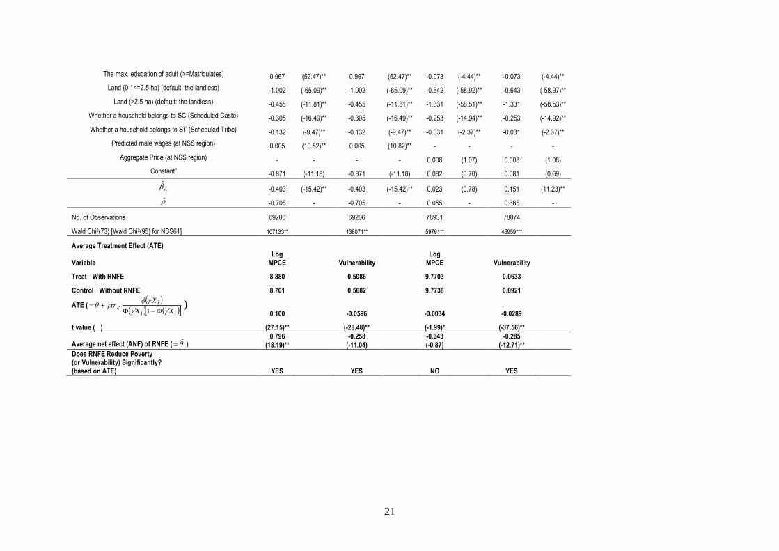
We have summarised the results of ATE at the bottom of Table 2. It is confirmed that
access to RNFE increases per capita consumption by 10% in 1993-4 on average, whilst it is
reduced by 0.34 % in 2004-5. That is, the consumption increasing effect (or the effect of
reducing consumption poverty) has weakened in recent years, which is consistent with
evidence from Vietnam. However, contrary to the results of Vietnam, vulnerability was
significantly reduced by participation in RNFE – by 5.96% in 1993-4 and by 2.89% (in terms
of the probability of falling into poverty in the next period). This is a substantial reduction. It
can be concluded that in India participation in RNFE is likely to reduce household
vulnerability significantly.

20
Table 2. The Results of Treatment Effects Model on the Effects of Participation in Rural Non-Farm Economy (RNFE) for Vietnam on Poverty and Vulnerability for India
NSS 50 (1993-4) NSS 61 (2004-5)
log per capita MPCE Vulnerability
log per capita MPCE Vulnerability
Coef. Z value Coef. Z value Coef. Z value Coef. Z value
Whether a household is headed by a female member - - - - 0.002 (0.25) -0.048 (-12.13)
Number of adult female members -0.307 (-115.68)** 0.132 (99.62)** -0.128 (-56.3)** 0.053 (45.11)**
Number of adult male members -0.276 (-112.92)** 0.128 (105.21)** -0.108 (-41.53)** 0.052 (40.13)**
Dependency Burden (share of household members under 15 or above 60) 2.208 (218.74)** -1.403 (-277.95)** 0.611 (82.67)** -0.216 (-56.77)**
Age of household head -0.963 (-11.51)** 0.987 (23.59)** 0.596 (8.15)** -0.194 (-5.14)**
Age squared 0.978 (11.19)** -0.886 (-20.27)** -0.248 (-3.43)** -0.049 (-1.30)
The max. education of adult (Primary) 0.065 (7.73)** -0.050 (-11.81)** 0.098 (16.89)** -0.081 (-27.80)**
The max. education of adult (Middle) 0.120 (11.84)** -0.114 (-22.05)** 0.244 (46.1)** -0.148 (-55.67)**
The max. education of adult (>=Matriculates) 0.184 (11.59)** -0.205 (-24.51)** 0.508 (97.08)** -0.193 (-71.39)**
Land (0.1<=2.5 ha) (default: the landless) 0.407 (29.08)** -0.176 (-23.75)** 0.056 (4.63)** -0.115 (-20.71)**
Land (>2.5 ha) (default: the landless) 0.206 (12.08)** -0.104 (-12.18)** 0.277 (13.26)** -0.215 (-22.36)**
Whether a household belongs to SC (Scheduled Caste) -0.136 (-16.15)** 0.090 (20.97)** -0.172 (-26.01)** 0.112 (34.36)**
Whether a household belongs to ST (Scheduled Tribe) -0.128 (-20.43)** 0.075 (23.58)** -0.132 (-30.73)** 0.072 (32.58)**
Average net effect of household member participation in
non-farm sector employment ( ) 0.796 (18.19)** -0.258 (-11.04)** -0.043 (-0.87) -0.285 (-12.71)**
Constant 7.982 (231.37) 1.056 (60.83) 9.602 (278.11) 0.366 (22.28)
Whether a household is headed by a female member - - - - -0.389 (-22.36)** -0.389 (-22.35)**
Number of adult female members -0.020 (-3.15)** -0.020 (-3.15)** 0.021 (2.84)** 0.021 (2.87)**
Number of adult male members -0.019 (-3.23)** -0.019 (-3.23)** 0.091 (13.09)** 0.091 (13.07)**
Dependency Burden (share of household members under 15 or above 60) -0.091 (-3.81)** -0.091 (-3.81)** -0.097 (-4.25)** -0.098 (-4.27)**
Age of household head -0.514 (-2.57)* -0.514 (-2.57)* -0.476 (-2.05)* -0.476 (-2.05)*
Age squared 0.760 (3.64)** 0.760 (3.64)** -0.293 (-1.25) -0.293 (-1.25)
The max. education of adult (Primary) 0.267 (14.88)** 0.267 (14.88)** 0.182 (12.0)** 0.182 (11.98)**
The max. education of adult (Middle) 0.422 (22.00)** 0.422 (22.00)** 0.162 (11.46)** 0.162 (11.45)**
21
The max. education of adult (>=Matriculates) 0.967 (52.47)** 0.967 (52.47)** -0.073 (-4.44)** -0.073 (-4.44)**
Land (0.1<=2.5 ha) (default: the landless) -1.002 (-65.09)** -1.002 (-65.09)** -0.642 (-58.92)** -0.643 (-58.97)**
Land (>2.5 ha) (default: the landless) -0.455 (-11.81)** -0.455 (-11.81)** -1.331 (-58.51)** -1.331 (-58.53)**
Whether a household belongs to SC (Scheduled Caste) -0.305 (-16.49)** -0.305 (-16.49)** -0.253 (-14.94)** -0.253 (-14.92)**
Whether a household belongs to ST (Scheduled Tribe) -0.132 (-9.47)** -0.132 (-9.47)** -0.031 (-2.37)** -0.031 (-2.37)**
Predicted male wages (at NSS region) 0.005 (10.82)** 0.005 (10.82)** - - - -
Aggregate Price (at NSS region) - - - - 0.008 (1.07) 0.008 (1.08)
Constant” -0.871 (-11.18) -0.871 (-11.18) 0.082 (0.70) 0.081 (0.69)
-0.403 (-15.42)** -0.403 (-15.42)** 0.023 (0.78) 0.151 (11.23)**
-0.705 - -0.705 - 0.055 - 0.685 -
No. of Observations 69206 69206 78931 78874
Wald Chi2(73) [Wald Chi2(95) for NSS61] 107133** 138071** 59761** 45959***
Average Treatment Effect (ATE)
Variable
Log
MPCE Vulnerability
Log
MPCE Vulnerability
Treat With RNFE 8.880 0.5086 9.7703 0.0633
Control Without RNFE 8.701 0.5682 9.7738 0.0921
ATE (
ii
i
XX
X
1)
0.100 -0.0596 -0.0034 -0.0289
t value ( ) (27.15)** (-28.48)** (-1.99)* (-37.56)**
Average net effect (ANF) of RNFE ( ) 0.796
(18.19)**
-0.258
(-11.04)
-0.043
(-0.87)
-0.285
(-12.71)**
Does RNFE Reduce Poverty (or Vulnerability) Significantly?
(based on ATE) YES YES NO YES

22
5. Concluding Observations
The present study examines whether participation in the rural non-farm sector employment
or involvement in activity in rural non-farm economy (RNFE) has any poverty-reducing or
vulnerability-reducing effect in Vietnam and India. To take account of sample selection bias
associated with RNFE, we applied treatment-effects model, a variant of Heckman sample
selection model.
It is found that log per capita consumption or log mean per capita expenditure (MPCE)
significantly increased in 2002 and 2004 for Vietnam and in 1993-4 for India. This is
consistent with poverty reducing role of accessing RNFE. However, in later years, this
statistically significant consumption poverty reducing effect disappeared. That is, it was no
longer statistically significant in 2006 for Vietnam and MPCE slightly reduced due to access
to RNFE in 2004-5 for India.
Access to RNFE significantly reduces vulnerability in India. This is important as a
significant number of households in rural India were found to be vulnerable to shocks in the
future (e.g. weather shocks, illness of household members, macro-economic slowdown).
Diversification of household activities into non-farm sector would reduce such risks. In sharp
contrast, in Vietnam, RNFE significantly increased vulnerability in 2002, but the effect
became statistically non-significant in 2004 and 2006.
As the results are mixed, we cannot offer a definitive conclusion, but some of the results
on poverty and vulnerability are consistent with the recent views that non-farm sector plays a
key role in helping poor agricultural households escape poverty, as emphasised by Knight et
al. (2009, 2010) in the context of rural China. Policy interventions designed to help
agricultural households diversify into non-farm sector activities (e.g. skill training;
microfinance) would potentially reduce not only poverty but also vulnerability.

23
References
Bliss C. and Stern, N., (1978) ‘Productivity, wages and nutrition: Part I: The theory’. Journal
of Development Economics, 5 (4), 331-362
Chaudhuri, S. 2003. Assessing vulnerability to poverty: concepts, empirical methods and
illustrative examples. mimeo, New York: Columbia University.
Chaudhuri, S., J. Jalan and A. Suryahadi. 2002. Assessing Household Vulnerability to
Poverty: A Methodology and Estimates for Indonesia. Columbia University Department
of Economics Discussion Paper No. 0102-52, New York: Columbia University.
Dasgupta, P. 1997. Nutritional status, the capacity for work, and poverty traps. Journal of
Econometrics 77, no.1 :5–37.
Dasgupta, P., and D. Ray, (1986) ‘Inequality as a determinant of malnutrition and
unemployment: Theory’, Economic Journal, 96: 1011–1034.
Dasgupta, P., and D. Ray, (1987) ‘Inequality as a determinant of malnutrition and
unemployment: Policy’, Economic Journal, 97: 177–188.
de Janvry, A., Sadoulet, E., and Nong, Z., (2005) ‘The role of non-farm incomes in reducing
rural poverty and inequality in China’, CUDARE Working Paper Series 1001, University
of California at Berkeley.
Foster, A. 1995. Household Savings and Human Investment Behaviour in Development,
Nutrition and Health Investment. The American Economic Review 85 :148–152.
Gaiha, R., and Imai, K., (2009) ‘Measuring Vulnerability and Poverty in Rural India’ in W.
Naudé, A. Santos-Paulino and M. McGillivray (Eds.), Vulnerability in Developing
Countries, United Nations University Press.
Gaiha, R., R. Jha and Vani S. Kulkarni (2012a) Diets, Malnutrition and Disease in India,
Oxford University Press. Forthcoming

24
Gaiha, R., Kaicker, N., Imai, K. and Thapa, G. (2012b) “Demand for Nutrients in India: An
Analysis Based on the 50th, 61st and 66th Rounds of the NSS”, IFAD, Rome, mimeo.
Greene, William H., (2003) Econometric Analysis 5th edition, Upper Saddle River, NJ:
Prentice-Hall.
Haggblade, S., Hazell, P., and Reardon, T., (2010) ‘The Rural Nonfarm Economy: Prospects
for Growth and Poverty Reduction’, World Development, 38(10), 1429–1441.
Heckman, J., (1979) ‘Sample selection bias as a specification error’, Econometrica 47, 153
Hoddinott, J. and A. Quisumbing. 2003a. Data Sources for Microeconometric Risk and
Vulnerability Assessments. Social Protection Discussion Paper Series No.0323, Washington
D.C.: The World Bank.
Hoddinott, J. and A. Quisumbing. 2003b. Methods for Microeconometric Risk and
Vulnerability Assessments. Social Protection Discussion Paper Series No.0324, Washington
D.C.: The World Bank.
Imai, K., (2011) ‘Poverty, undernutrition and vulnerability in rural India: Role of rural public
works and food for work programmes’, International Review of Applied Economics,
25(6), 669–691.
Imai, K., Gaiha, R. and Kang, W., (2011) ‘Poverty Dynamics and Vulnerability in Vietnam’ ,
Applied Economics, 43(25), pp. 3603-3618.
Imai, K., Annim, S., Gaiha, R., and Kulkarni, V., (2012a) ‘Nutrition, Activity Intensity and
Wage Linkages: Evidence from India’, DP2012-10, Kobe University.
Imai, K., Annim, S., Gaiha, R., and Kulkarni, V., (2012b) ‘Does Women’s Empowerment
Reduce Prevalence of Stunted and Underweight Children in Rural India?’, DP2012-11,
Kobe University.
Jha, R., Gaiha, R., and Sharma, A., (2009) ‘Calorie and Micronutrient Deprivation and
Poverty Nutrition Traps in Rural India’, World Development, 37(5): 982–991.
25
Knight, J., Shi, L. and Quhend, D,. (2009) ‘Education and the Poverty Trap in Rural China:
Setting the Trap’, Oxford Development Studies, 37(4), 311-332.
Knight, J., Shi, L. and Quhend, D., (2010) ‘Education and the Poverty Trap in Rural China:
Closing the Trap’, Oxford Development Studies, 38(1), 1-24.
Lanjouw, J., and Lanjouw, P., (2001) ‘The rural non-farm: sector: issues and evidence from
developing countries’, Agricultural Economics, 26, 1-23.
Maddala, G. S., (1983) Limited-dependent and Qualitative Variables in Econometrics.
Cambridge: Cambridge University Press.
Owusu, V., Abdulai, A., Abdul-Rahman, S., (2011) ‘Non-farm work and food security
among farm households in Northern Ghana’, Food Policy 36, 108–118.
Reardon, T., Stamoulis, K., Lanjouw, P., and Balisacan, A., (2000) ‘Effects of Non-Farm
Employment on Rural Income Inequality in Developing Countries: An Investment
Perspective’, Journal of Agricultural Economics, 51(2), 266-288.
Scandizzo, P, Gaiha, R. and Imai, K., (2009) ‘Option Values, Switches and Wages - An
Analysis of the Employment Guarantee Scheme in India’, Review of Development
Economics, 13(2), pp.248-263.
van de Walle, D., and Cratty, D. (2004) ‘Is the emerging non-farm market economy the route
out of poverty in Vietnam?,’ The Economics of Transition, 12(2), 237-274.
26
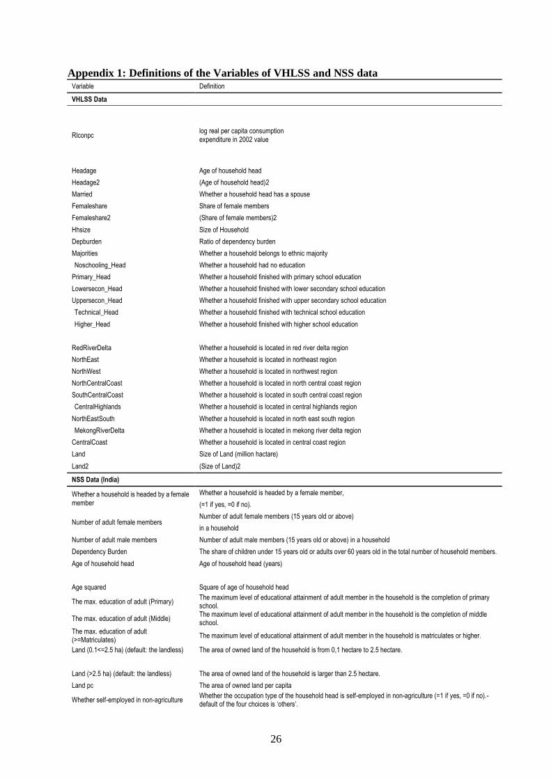
Appendix 1: Definitions of the Variables of VHLSS and NSS data Variable Definition
VHLSS Data
Rlconpc log real per capita consumption
expenditure in 2002 value
Headage Age of household head
Headage2 (Age of household head)2
Married Whether a household head has a spouse
Femaleshare Share of female members
Femaleshare2 (Share of female members)2
Hhsize Size of Household
Depburden Ratio of dependency burden
Majorities Whether a household belongs to ethnic majority
Noschooling_Head Whether a household had no education
Primary_Head Whether a household finished with primary school education
Lowersecon_Head Whether a household finished with lower secondary school education
Uppersecon_Head Whether a household finished with upper secondary school education
Technical_Head Whether a household finished with technical school education
Higher_Head Whether a household finished with higher school education
RedRiverDelta Whether a household is located in red river delta region
NorthEast Whether a household is located in northeast region
NorthWest Whether a household is located in northwest region
NorthCentralCoast Whether a household is located in north central coast region
SouthCentralCoast Whether a household is located in south central coast region
CentralHighlands Whether a household is located in central highlands region
NorthEastSouth Whether a household is located in north east south region
MekongRiverDelta Whether a household is located in mekong river delta region
CentralCoast Whether a household is located in central coast region
Land Size of Land (million hactare)
Land2 (Size of Land)2
NSS Data (India)
Whether a household is headed by a female
member
Whether a household is headed by a female member,
(=1 if yes, =0 if no).
Number of adult female members Number of adult female members (15 years old or above)
in a household
Number of adult male members Number of adult male members (15 years old or above) in a household
Dependency Burden The share of children under 15 years old or adults over 60 years old in the total number of household members.
Age of household head Age of household head (years)
Age squared Square of age of household head
The max. education of adult (Primary) The maximum level of educational attainment of adult member in the household is the completion of primary school.
The max. education of adult (Middle) The maximum level of educational attainment of adult member in the household is the completion of middle school.
The max. education of adult (>=Matriculates)
The maximum level of educational attainment of adult member in the household is matriculates or higher.
Land (0.1<=2.5 ha) (default: the landless) The area of owned land of the household is from 0,1 hectare to 2.5 hectare.
Land (>2.5 ha) (default: the landless) The area of owned land of the household is larger than 2.5 hectare.
Land pc The area of owned land per capita
Whether self-employed in non-agriculture Whether the occupation type of the household head is self-employed in non-agriculture (=1 if yes, =0 if no).- default of the four choices is ‘others’.

27
Whether agricultural labour Whether the occupation type of the household head is agricultural labour
(=1 if yes, =0 if no).
Whether non-agricultural labour Whether the occupation type of the household head is labour in non-agriculture (=1 if yes, =0 if no).
Whether self-employed in agriculture Whether the occupation type of the household head is self-employed in agriculture (=1 if yes, =0 if no).
Whether a household belongs to SC (Scheduled Caste)
Whether a household belongs to SC (Scheduled Caste) (=1 if yes, =0 if no).
Whether a household belongs to ST (Scheduled Tribe)
Whether a household belongs to ST (Scheduled Tribe) (=1 if yes, =0 if no).
RPW Whether a household has access to Rural Public Works.
FFW Whether a household has access to Food for Work Programme.
Predicted agricultural wage rate for males Agricultural Wage Rate for male workers averaged at NSS region.
Poor Whether the household per capita expenditure is under the national poverty line for rural areas.
poor (calorie based) Whether the household is undernourished in terms of calorie intakes.
poor (protein based) Whether the household is undernourished in terms of protein intakes.
Vulnerability Measure (based on 100% income poverty line)
Whether the household is vulnerable
(based on 100% of the national poverty line).
Vulnerability Measure (based on 80%
income poverty line) Whether the household is vulnerable (based on 80% of the national poverty line).
Vulnerability Measure (based on 120% income poverty line)
Whether the household is vulnerable (based on 120% of the national poverty line).

28
Appendix 2: Wage Equations for male and female workers in rural areas based on NSS
data in 1993 and 2004 1993 2004
Male
wage Female Wage
Male Wage
Female Wage
Coef. Coef. Coef. Coef.
(t value) (t value) (t value) (t value)
Land Owned 0.349 -0.324 0.00 -0.082
(0.98) (4.86)** (2.39)* (8.35)**
Scheduled Tribe (ST) dummy (ST=1, otherwise=0) -322.569 -1,018.14 -121.41 -108.96
(0.87) (4.08)** (9.13)** (7.53)**
Scheduled Caste (SC) dummy (SC=1, otherwise=0) -2,177.57 -381.166 - -
(7.95)** (1.89)
non-agricultural self employment dummy (non-agricultural
self employment=1 otherwise) 7,216.57 2,324.92 1,859.26 566.23
(10.27)** (5.49)** (68.44)** (21.97)**
agricultural self employment dummy (agricultural self employment=1 otherwise=0)
7,899.48 5,204.41 2,196.08 880.79
(15.13)** (14.37)** (69.07)** (22.83)**
Muslim dummy(Muslim=1, otherwise=0) 746.744 185.894 113.494 -330.9
(1.61) (0.46) (5.59)** (10.79)**
Age 662.822 204.695 139.625 49.933
(8.65)** (3.65)** (37.08)** (10.15)**
Age2 -4.072 -1.257 -1.638 -0.637
(4.17)** (1.69) (39.07)** (10.24)**
Whether is literate, but has not completed primary school 3,542.99 2,126.39 92.081 -205.98
(12.71)** (7.36)** (5.10)** (8.72)**
Whether mother completed primary school 7,518.66 3,208.70 175.043 -227.04
(23.01)** (7.49)** (9.45)** (9.53)**
Whether mother completed middle school 14,163.75 10,200.92 360.514 -192.21
(29.57)** (8.09)** (19.49)** (7.37)**
Whether completed secondary or higher secondary school 35,055.00 38,201.86 810.913 201.04
(56.87)** (26.88)** (33.86)** (5.63)**
Whether completed higher education 57,151.06 53,253.26 1,473.09 1,004.51
(47.65)** (17.32)** (64.15)** (20.43)**
Constant -2,171.00 4,216.78 -2,940.20 -1,749.97
(1.50) (4.18)** (34.97)** (16.65)**
Observations 33720 15849 67168 59221
Robust z-statistics in parentheses
* significant at 5% level; ** significant at 1% level

29
Appendix 3: Deriving Vulnerability Measure16
Vulnerability measure as an expected poverty is specified as:
zcPrVVEP 1t,iitit (A-1)
where vulnerability of household i at time t, itV , is the probability that the i-th household’s
level of consumption at time t+1, 1t,ic , will be below the poverty line, z.
Three limitations, amongst others, should be noted in our measure of vulnerability.
First, the present analysis is confined to a consumption (used synonymously with income)
threshold of poverty. Second, our measure of vulnerability in terms of the probability of a
household’s consumption falling below the poverty threshold in the future is subject to the
choice of a threshold. Third, while income/consumption volatility underlies vulnerability, the
resilience in mitigating welfare losses depends on assets defined broadly-including human,
physical and social capital. A household with inadequate physical or financial asset or
savings, for example, may find it hard to overcome loss of income. This may translate into
lower nutritional intake and rationing out of its members from the labour market (Dasgupta,
1997; Foster, 1995). Lack of physical assets may also impede accumulation of profitable
portfolios under risk and generate poverty traps.
The consumption function is estimated by the equation (A-2).17
iii eXc ln (A-2)
where ic is log of real per capita household consumption (for Vietnam) and mean per capita
consumption (MPCE) (i.e. food and non-food consumption expenditure) (for India) for the
household and X is a vector of observable household characteristics and other determinants
of consumption. It is further assumed that the structure of the economy is relatively stable
over time and, hence, future consumption stems solely from the uncertainty about the
16
This Appendix is based on Imai (2011) and Imai et al. (2011). 17
We have used White-Huber sandwich estimator to overcome heteroscedasticity in the sample.

30
idiosyncratic shocks, ie . It is also assumed that the variance of the disturbance term depends
on:
i
2
i,e X (A-3)
The estimates of and are obtained using a three-step feasible generalized least
squares (FGLS)18
. Using the estimates and , we can compute the expected log
consumption and the variance of log consumption for each household as follows.
ˆX]XC[lnE iii (A-4)
ˆX]XC[lnV iii (A-5)
By assuming icln as normally distributed and letting denote the cumulative density
function of the standard normal distribution, the estimated probability that a household will
be poor in the future (say, at time t+1) is given by:
ˆX
ˆXzlnXzlnclnrPvPEV
i
iiiii
(A-6)
This is an ex ante vulnerability measure that can be estimated with cross-sectional
data. Note that this expression also yields the probability of a household at time t becoming
poor at t+1 given the distribution of consumption at t.
A merit of this vulnerability measure is that it can be estimated with cross-sectional data.
However, it correctly reflects a household’s vulnerability only if the distribution of
consumption across households, given the household characteristics at time t, represents
time-series variation of household consumption. Hence this measure requires a large sample
in which some households experience positive shocks while others suffer from negative
18
See Chaudhuri (2003), Chaudhuri et al. (2002), and Hoddinott and Quisumbing (2003b) for
technical details.

31
shocks. Also, the measure is unlikely to reflect unexpected large negative shocks (e.g., Asian
financial crisis), if we use the cross-section data for a normal year.