does foreign debt contribute to economic growth? arxiv
TRANSCRIPT

Does Foreign Debt Contribute to Economic
Growth?∗
Tomoo Kikuchia and Satoshi Tobeb
aSchool of Asia-Pacific Studies, Waseda UniversitybSchool of Policy Studies, Kwansei Gakuin University
September 23, 2021
Abstract
We study the relationship between foreign debt and GDP growth using a panel
dataset of 122 countries from 1980 to 2015. We find that economic growth
correlates positively with foreign debt and that the relationship is causal in
nature by using the sovereign credit default swap spread as an instrumental
variable. Furthermore, we find that foreign debt increases investment and
then GDP growth in subsequent years. Our findings suggest that sovereign
default risks are responsible for “upstream” capital flows that contribute to
GDP growth in OECD countries.
Keywords: foreign debt; upstream capital flows; GDP growth; investment;
sovereign credit default swap
JEL Classification: F21; F34; O16
∗We would like to thank seminar participants at Korea University, Peking University,
Sichuan University, and Waseda University and acknowledge valuable comments from Wen-
tao Fu, Jinill Kim, Jong-Wha Lee, Cheolbeom Park, Kwanho Shin, Yong Wang, Lei Zhang
and Lijung Zhu, and financial support from Korea University (K2009811 and K1922081) and
BrainKorea21 Plus (K1327408 and T192201). Corresponding author: Tomoo Kikuchi. Email:
1
arX
iv:2
109.
1051
7v1
[ec
on.G
N]
22
Sep
2021

1 Introduction
Since financial globalization started accelerating in 1980’s, global imbalances have
emerged (see Mendoza et al., 2009). Between 1980 and 2020 the sum of current
account balances of the US amounts to –$12514 billion, which is the largest cumula-
tive deficit among all countries, while that of China amounts to $3725 billion.1 This
means that the US has imported while China has exported capital over the past
40 years. The law of diminishing returns implies that capital—ceteris paribus—
would flow from rich countries where the marginal product of capital is low to poor
countries where it is high. Therefore, in the neoclassical model poor countries are
supposed to import and rich countries are supposed to export capital. However,
Lucas (1990) observed that capital does not flow from rich to poor countries just as
the example of the US and China shows.
Since Lucas’ seminal work, the literature has decomposed capital flows in the finan-
cial account to examine the effects of each flow. It is well-established that foreign
direct investment (FDI) contributes to economic growth in developing countries with
a high level of human capital in Borensztein et al. (1998) or developed financial mar-
kets in Alfaro et al. (2004). The finding seems to be consistent with the neoclassical
model. On the other hand, several studies find that upstream capital flows are
caused by emerging economies that accumulate foreign reserves (e.g., Gourinchas
and Rey, 2007; Mendoza et al., 2009; Gourinchas and Jeanne, 2013; Alfaro et al.,
2014). However, the relationship between portfolio investment and economic growth
remains elusive.2
This paper investigates the relation between foreign debt—the debt instrument in
portfolio investment—and GDP growth using a panel dataset covering 122 countries
from 1980 to 2015. Figure 1 shows that net foreign debt of OECD countries largely
mirrors foreign reserve holdings of non-OECD countries.3 It is surprising to see
1Data of China’s current account balances are missing for 1980 and 1981.2In theoretical models with no FDI, financial frictions may limit domestic investment and lead
to upstream (portfolio investment) flows from “poor” countries to “rich countries” and sustain the
cross-country inequality when financial markets are integrated globally (e.g. Matsuyama, 2004;
Kikuchi and Stachurski, 2009; Kikuchi et al., 2018). If FDI is allowed, investors in rich countries
could circumvent host-country financial frictions and invest in poor countries.3The sum of net foreign debt across all countries in the world must be zero except for the
2
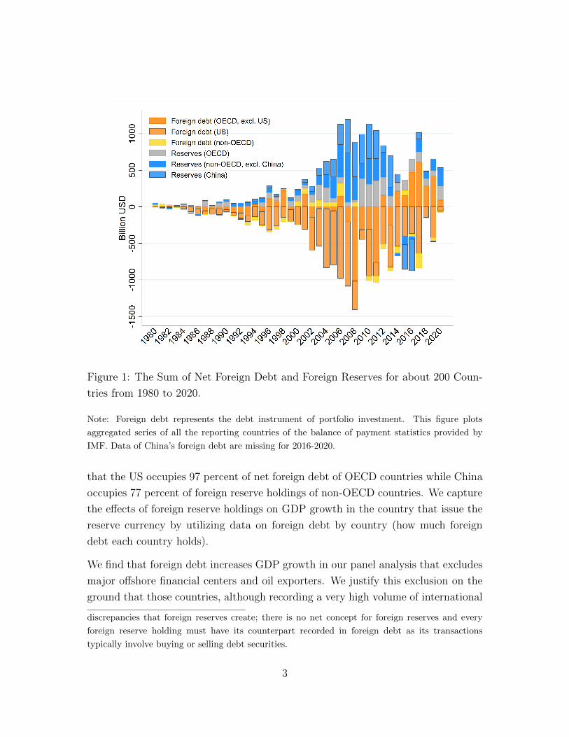
Figure 1: The Sum of Net Foreign Debt and Foreign Reserves for about 200 Coun-
tries from 1980 to 2020.
Note: Foreign debt represents the debt instrument of portfolio investment. This figure plots
aggregated series of all the reporting countries of the balance of payment statistics provided by
IMF. Data of China’s foreign debt are missing for 2016-2020.
that the US occupies 97 percent of net foreign debt of OECD countries while China
occupies 77 percent of foreign reserve holdings of non-OECD countries. We capture
the effects of foreign reserve holdings on GDP growth in the country that issue the
reserve currency by utilizing data on foreign debt by country (how much foreign
debt each country holds).
We find that foreign debt increases GDP growth in our panel analysis that excludes
major offshore financial centers and oil exporters. We justify this exclusion on the
ground that those countries, although recording a very high volume of international
discrepancies that foreign reserves create; there is no net concept for foreign reserves and every
foreign reserve holding must have its counterpart recorded in foreign debt as its transactions
typically involve buying or selling debt securities.
3

financial transactions, might distort our analysis because they channel a very small
portion of capital inflows into domestic investment - the channel we would like to
explore in this paper. In fact, we find that foreign debt increases investment and
then GDP growth in subsequent years by employing the local projection analysis
developed by Jorda (2005). This indicates that foreign debt contributes to GDP
growth through capital accumulation.
Using the sovereign credit default swap (CDS) spread as an instrumental variable
(IV) we find the relationship between foreign debt and GDP growth to be causal in
nature. (We refer to the sovereign credit default swap as the CDS throughout the
paper.) The CDS spread is the cost that investors pay to hedge against sovereign
default risks. Thus, the predicted values in the first stage of panel IV regression can
be interpreted as changes in foreign debt caused by exogenous supply-side shocks.
To the best of our knowledge we are the first to identify how sovereign CDS spreads
affect investment and GDP growth via foreign debt in a large panel dataset.
Lastly, we divide our sample into OECD and non-OECD countries to relate our
results to upstream capital flows and global imbalances as observed in Figure 1.
We find that the CDS spread is lower and foreign debt is higher in OECD than
non-OECD countries on average.4 Our model excluding foreign debt but including
common control variables used in the growth regression literature underestimates
GDP growth of OECD countries. The inclusion of foreign debt increases the ex-
planatory power of our model for GDP growth in OECD countries by 2.2 percent.
Hence, the novel channel between foreign debt and growth we identify via the CDS
spread points to the “real” effects of the “exorbitant privilege” the US and other
OECD countries have (c.f., Gourinchas and Rey, 2007). We conclude that sovereign
default risks are responsible for upstream capital flows that contribute to GDP
growth through capital accumulation in OECD countries.
The positive relationship between foreign debt and GDP growth we find is the
opposite of what many others find for developing countries. For example, Pattillo
et al. (2002) finds that the effect of foreign debt on per capita growth is negative
among average developing countries. Similarly, Clements et al. (2003) finds that high
levels of debt can depress economic growth in low-income countries. Those findings
4Demirguc-Kunt et al. (2013) finds that securities markets become more important than banks
as the economy develops.
4

are in line with debt overhang problems in low-income economies where a country’s
debt service burden to foreign lenders is so heavy that it creates disincentives to
invest in the country (see Krugman, 1988). We differ from this line of literature in
that 1) our sample covers a wide range of countries from low-income to high-income
countries; 2) our IV approach controls for the incentives to invest in a country; and
3) our battery of controls such as regulatory quality and the government debt to
GDP ratio accounts for the credibility of debtors. In other words, we control for
unfavorable conditions in countries that suffer from debt overhang problems and
analyze the effect of foreign debt on growth in a more general setup.
Our work may also be contrasted with the literature that finds a negative relation-
ship between public debt and growth (see Reinhart and Rogoff, 2010). Examining
different samples of countries and periods, most works in the literature confirm a
negative relationship between debt and growth (see Reinhart et al., 2012, for a sur-
vey). Our work differs from them as our main independent variable is foreign debt,
i.e., debt that a country owes to foreigners (both public and private entities). Given
home bias as in Feldstein and Horioka (1979) foreigners are more responsive to
shocks in international capital markets than domestic residents are. In other words,
investors are more selective when investing internationally than domestically, and
therefore issuing debt domestically is fundamentally different from issuing debt in-
ternationally. Those differences, which we capture implicitly through our controls
and IV approach, must be responsible for the positive relationship between foreign
debt and growth.
The rest of the paper is organized as follows. Section 2 describes the panel data
and reports the results of the baseline model. Section 3 investigates the investment
channel and Section 4 the dynamic effects of foreign debt. Section 5 relates our
findings to upstream capital flows and global imbalances. Section 6 concludes.
5

2 GDP Growth and Foreign Debt
2.1 Panel Data
We construct a country-level unbalanced panel dataset covering 122 countries from
1980 to 2015.5 The panel data used in the baseline analysis cover 95 percent of
world GDP on average throughout the sample period. In addition to the full sample,
we use two sub-samples. The first sub-sample, as discussed later, excludes outlier
countries from the full sample. This sub-sample covers 96 countries from 1980 to
2015 representing 81 percent of world GDP on average. The second sub-sample used
for instrumental variable regressions has a more limited sample size due to data
availability of the instrument and controls. The sample covers 50 countries from
1997 to 2015 representing 48 percent of world GDP on average. The robustness of
results using different samples shows the generality of our estimation results.
The baseline model uses real GDP growth as the key dependent variable. GDP is
measured in a constant local currency unit and provided in the World Development
Indicator (WDI) database by the World Bank. We also use investment growth as
a dependent variable in our additional analysis. Total investment is measured in a
constant local currency unit and provided in the WDI database. Total investment
can be decomposed into private and public investment, each measured in a constant
US dollar unit rather than a local currency unit due to data availability. The series
are provided by the IMF. 6
The key right-hand-side variable is foreign debt normalized by GDP. Throughout
this paper foreign debt denotes the debt instrument of portfolio investment, which
captures international transactions of corporate and government debt provided in
the International Financial Statistics by the IMF. The series measure net capital
inflows (gross inflows minus gross outflow). The balance of payments statistics
also reports the debt instrument in a sub-category of other investment flows. We
do not include the series in foreign debt as it mainly captures cross-border banking
5See Table 8 for the list of countries.6We confirmed that main results hold when we use real GDP or investment growth measured
in a constant US dollar unit. However, we mainly use the series measured in a local currency unit
to eliminate the valuation effects caused by changes in exchange rates as much as possible.
6
activities such as bank lending and deposit transactions, which is not directly related
to investment.
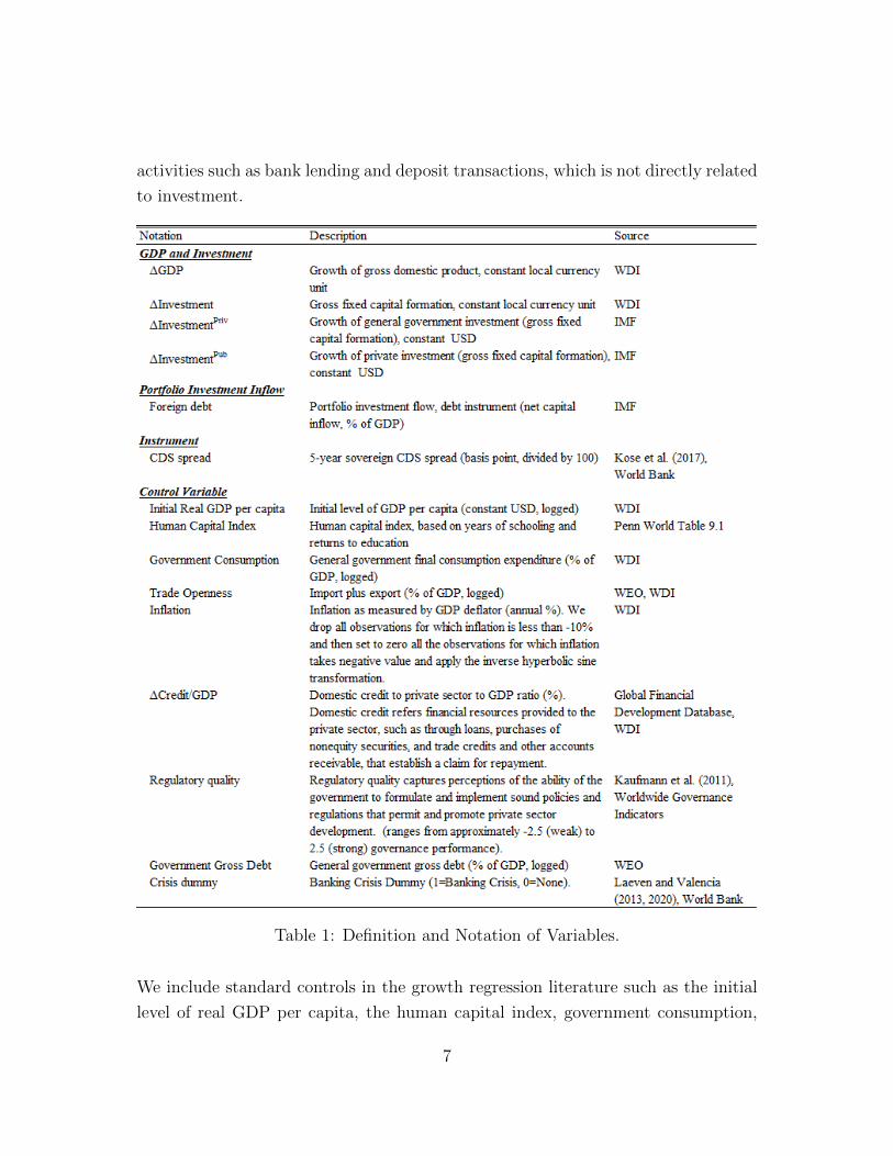
Table 1: Definition and Notation of Variables.
We include standard controls in the growth regression literature such as the initial
level of real GDP per capita, the human capital index, government consumption,
7

trade openness, and the inflation rate (e.g. Arcand et al., 2015; Durlauf et al., 2005).
The details are summarized in Table 1.
2.2 The Baseline Model
The baseline model investigates the relationship between foreign debt and GDP
growth. There are two groups of countries that require a special treatment. The
first group contains offshore financial centers that record large transactions in inter-
national financial markets but typically re-invest capital inflows in third countries.
The second group contains oil exporters that invest their oil revenues in foreign
equity or debt and record large current account surplus (i.e., net capital outflow).
For both groups, capital inflows are not a source for domestic investment, which is
the channel we would like to explore. We identify 14 countries as offshore financial
centers following Lane and Milesi-Ferretti (2018) and 13 countries as major oil ex-
porters, whose time-series average of the oil rents to GDP ratio exceeds 8 percent.
The identified countries are listed in Tables 8 and 9.
The summary statistics shows that the offshore financial centers and oil exporters
are indeed outliers in our sample. Table 2 reports the cross-sectional summary
statistics of FDI and portfolio investment. In the full sample reported in panel A,
the standard deviation, minimum and maximum of portfolio investment are much
larger than those of FDI. For example, the standard deviation of portfolio investment
is 18.444, which is over three times larger than that of FDI (=5.471). Panels B and
C show that the large values of portfolio investment are attributable to the offshore
financial centers and oil exporters, who can work as noisy observations and lead
to inaccurate results. Moreover, panel C shows that total portfolio investment and
foreign debt have similar mean, standard deviation, minimum and maximum that
are different from those of equity instrument. This corroborates our strategy to
focus on foreign debt as the key driver of portfolio investment.
The baseline model is
∆GDPi,t = β1Foreign debti,t + β2Foreign debti,t ×DumNormal
+ ΓXi,t−1 + δi + γt + εi,t (1)
8
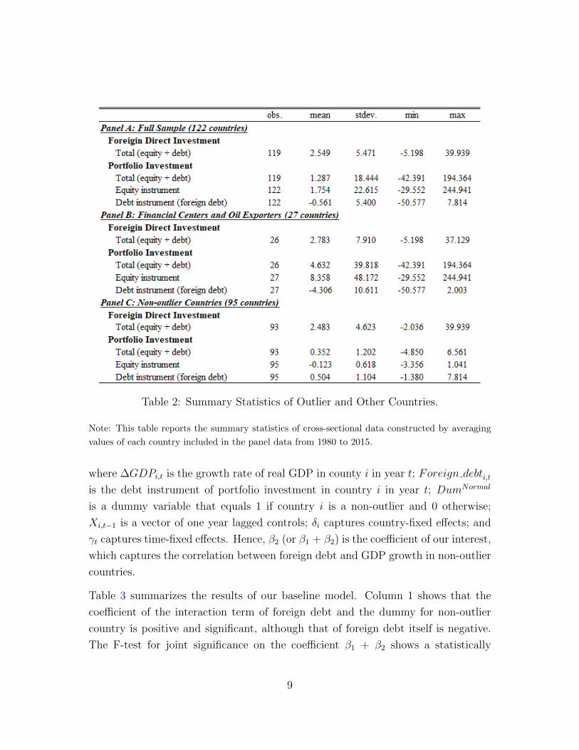
Table 2: Summary Statistics of Outlier and Other Countries.
Note: This table reports the summary statistics of cross-sectional data constructed by averaging
values of each country included in the panel data from 1980 to 2015.
where ∆GDPi,t is the growth rate of real GDP in county i in year t; Foreign debti,tis the debt instrument of portfolio investment in country i in year t; DumNormal
is a dummy variable that equals 1 if country i is a non-outlier and 0 otherwise;
Xi,t−1 is a vector of one year lagged controls; δi captures country-fixed effects; and
γt captures time-fixed effects. Hence, β2 (or β1 + β2) is the coefficient of our interest,
which captures the correlation between foreign debt and GDP growth in non-outlier
countries.
Table 3 summarizes the results of our baseline model. Column 1 shows that the
coefficient of the interaction term of foreign debt and the dummy for non-outlier
country is positive and significant, although that of foreign debt itself is negative.
The F-test for joint significance on the coefficient β1 + β2 shows a statistically
9

significant sign. This indicates that an increase in foreign debt is associated with
an increase in GDP growth for non-outlier countries. The result remains unchanged
when we exclude the outlier countries from the sample (column 2) or when we
include control variables (columns 3-4). Notably, the size of coefficients for non-
outlier countries is similar in columns 1 and 3 and in columns 2 and 4 suggesting
robustness of the results.
Table 3: Baseline Result Controlling Outlier Countries.
Note: The dependent variable is real GDP growth. The independent variable is foreign debt
(the debt instrument of portfolio investment divided by GDP) and its interaction term with the
non-outlier country dummy. Control variables are the lag of human capital index, government
consumption to GDP ratio (logged), trade openness (logged), the inflation rate, and initial level
of GDP per capita (logged). The sample used in columns 2 and 4 excludes 27 outlier countries.
Standard errors in parenthesis are clustered on country. *** p<0.01, ** p<0.05, * p<0.1
2.3 The Panel Instrumental Variable Approach
The baseline model in the previous section shows that higher foreign debt is asso-
ciated with higher GDP growth in non-outlier countries. This section employs an
instrumental variable (IV) approach to reduce concerns on endogeneity such as the
reverse causality between foreign debt and GDP growth. For example, higher GDP
10

growth may attract foreign capital because of higher demand for capital, which
would support a positive relation between GDP growth and foreign debt. This con-
cern arises as the baseline model may capture the effects of miscellaneous valuations
of foreign debt, instead of identifying exogenous shocks of foreign debt.
The panel IV analysis using an external instrument will help identify exogenous
shocks and reduce the endogeneity concerns. To this end, we require an instrument
that 1) correlates with foreign debt, but 2) is orthogonal to the error term. We
choose the sovereign credit default swap (CDS) spread as an instrument for foreign
debt. The data for the CDS spread are available from 1997 to 2015 provided by
Kose et al. (2017) and the World Bank. The CDS spread measures the cost for
investors to hedge against the sovereign default risk of a country. Hence, the CDS
spread naturally correlates with foreign debt. For example, an increase in the CDS
spread would lead to an decrease in foreign debt in a country because investors
would reduce demand for securities that are considered more risky. Regarding or-
thogonality to the error term, we might be concerned about a positive correlation
between fundamentals and the CDS spread. For example, an increase of current
GDP may reduce concerns on debt sustainability of a country decreasing the CDS
spread. If this were true, the CDS spread would correlate with the error term and
be an invalid instrument.
We present two arguments why we think that the CDS spread is orthogonal to the
error term. First, the CDS spread is a forward-looking variable, and therefore the
current economic variables including GDP growth must be irrelevant to the CDS
spread. For example, consider a case where GDP growth is caused by a positive
productivity shock. In this case GDP growth might increase or decrease the CDS
spread depending on how long the effects of the shock are expected to last. Second,
it is not GDP growth itself but the underlying causes for GDP growth that are
relevant to the CDS spread. For example, if GDP growth is caused by an increase
in government expenditure, investors might worry about the sustainability of debt
and the CDS spread might increase. This might be more likely for a country with a
high level of government debt. On the other hand, consider a country that is hit by
a permanent positive productivity shock. This may improve sustainability of debt
and decrease the CDS spread in the country. Hence, GDP growth, depending on its
underlying causes, can either increase or decrease the CDS spread. Therefore, we
11

assume that the CDS spread is randomly assigned to GDP growth across countries
and years guaranteeing orthogonality of the instrument to the error term.
With our IV estimation strategy we can identify supply-push effects of foreign debt
unrelated to demand factors in capital recipient countries. We employ two-stage
least squares (2SLS). In the first stage we regress foreign debt on the CDS spread
and controls to obtain the fitted values of foreign debt. The CDS spread is the cost
for investors to hedge against the sovereign risk, and thus contains supply-side infor-
mation such as willingness of investors to invest in a country. Therefore, the fitted
values estimated in the first stage can be interpreted as changes in foreign debt that
are caused by exogenous supply-side shocks. In the second stage, we regress GDP
growth on the fitted values. Hence, our panel IV regression identifies the supply-
push effects of foreign debt on GDP growth providing structural interpretation of
estimation results.
Figure 2 shows partial correlation between the CDS spread and foreign debt sketch-
ing the first stage regression. Both variables are residualized by the controls used in
Table 3 as well as country- and time-fixed effects. The scatter plots suggest that the
CDS spread predicts dynamics of foreign debt well: higher sovereign default risks,
which are not explained by observable factors and fixed effects, are associated with
smaller foreign debt. From the viewpoint of portfolio analysis investors are inclined
to reduce demand for securities that are considered more risky. We confirm this
negative relation in the formal analysis reported in Table 4.
Table 4 summarizes the results of the panel IV analysis. Here, we use the sub-
sample excluding the outlier countries because we can not set the instrument (the
CDS spread) for both foreign debt and the interaction term of foreign debt and
a dummy for non-outlier countries. Column 1 shows the results without control
variables. In the first stage, the coefficient of the CDS spread on foreign debt is
negative and significant suggesting that a lower sovereign default risk is associated
with higher foreign debt as expected. More importantly, the coefficient of foreign
debt on GDP growth is positive and significant in the second stage. One percentage
point increase in foreign debt leads to a 0.212 percentage point increase in real GDP.
The coefficient is over two times larger than the one estimated by the standard fixed-
effect estimation with the same sub-sample shown in column 2. The larger estimate
suggests that there is a downward bias in the baseline analysis possibly caused by
12
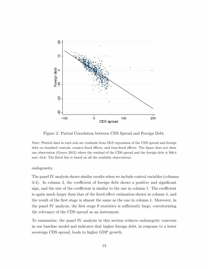
Figure 2: Partial Correlation between CDS Spread and Foreign Debt.
Note: Plotted data in each axis are residuals from OLS regressions of the CDS spread and foreign
debt on standard controls, country-fixed effects, and time-fixed effects. The figure does not show
one observation (Greece 2012) where the residual of the CDS spread and the foreign debt is 508.4
and -54.6. The fitted line is based on all the available observations.
endogeneity.
The panel IV analysis shows similar results when we include control variables (columns
3-4). In column 3, the coefficient of foreign debt shows a positive and significant
sign, and the size of the coefficient is similar to the one in column 1. The coefficient
is again much larger than that of the fixed-effect estimation shown in column 4, and
the result of the first stage is almost the same as the one in column 1. Moreover, in
the panel IV analysis, the first stage F-statistics is sufficiently large, corroborating
the relevance of the CDS spread as an instrument.
To summarize, the panel IV analysis in this section reduces endonegeity concerns
in our baseline model and indicates that higher foreign debt, in response to a lower
sovereign CDS spread, leads to higher GDP growth.
13

Table 4: Panel Instrumental Variable Approach (2SLS).
Note: The dependent variable is real GDP growth. The endogenous or independent variable is
foreign debt (the debt instrument of portfolio investment divided by GDP), instrumented with the
sovereign CDS spread in columns 1 and 3. Control variables are the lag of human capital index,
government consumption to GDP ratio (logged), trade openness (logged), inflation rate, and initial
level of GDP per capita (logged). Standard errors in parenthesis are clustered on country. ***
p<0.01, ** p<0.05, * p<0.1
2.4 Robustness
In the panel IV regression in Section 2.3 we might be concerned that the sovereign
CDS spread affects GDP growth through a channel other than foreign debt. In
that case, we must include the additional variable capturing the channel in our
specification. Financial crises might present such a channel. When a financial crisis
occurs, the sovereign default risk increases as GDP is expected to decrease, which in
turn decreases foreign debt. In such a case, the CDS spread is systematically related
to GDP growth. Therefore, we follow Laeven and Valencia (2013, 2020) to include
a banking crisis dummy in the following analysis. Similarly, the government debt
to GDP ratio might present another channel. Countries with higher government
debt tend to have a higher sovereign CDS spread and lower GDP growth due to
a debt overhang problem (e.g., Reinhart and Rogoff, 2010). Thus, we also include
14

the government gross debt to GDP ratio as an additional control. Furthermore,
to reduce concerns about omitted variable bias, we include the regulatory quality
index estimated by Kaufmann et al. (2011) and the growth of the private credit to
GDP ratio, both of which correlate with foreign debt and GDP growth as additional
controls.
Table 5: Robustness (2SLS).
Note: The dependent variable is real GDP growth. The endogenous variable is foreign debt (the
debt instrument of portfolio investment divided by GDP) instrumented with the sovereign CDS
spread (columns 1–4) or the sovereign rating (column 5). Control variables are the lag of human
capital index, government consumption to GDP ratio (logged), trade openness (logged), inflation
rate, initial level of GDP per capita (logged), banking crisis dummy, general government gross debt
to GDP ratio (logged), regulatory quality, and growth of private credit to GDP ratio. Standard
errors in parenthesis are clustered on country. *** p<0.01, ** p<0.05, * p<0.1
Table 5 summarizes the results of including the additional controls. The specification
in column 1 includes the banking crisis dummy and the government debt to GDP
15

ratio showing that our main results hold. The CDS spread is negatively correlated
with foreign debt in the first stage, and its coefficient is positive and significant in
the second stage. The results remain unchanged if we add the regulatory quality
index (column 2), the growth of the credit to GDP ratio (column 3), or both (column
4). The size of the coefficients is fairly stable across the specifications ranging from
0.165 to 0.185.
Similar to the CDS spread, the sovereign debt rating may be another valid instru-
ment for foreign debt. This is because the rating also captures the sovereign default
risk of a country and correlates with foreign debt of the country. We perform a
panel IV analysis using both the CDS spread and the sovereign rating as instru-
ments, which enables us to conduct an over-identification test. As shown in column
5 of Table 5, the main results hold. More importantly, the over-identification test
confirms that we can not reject the null hypothesis that the excluded instruments
are exogenous, although the first stage F-statistics becomes much smaller. This
result corroborates the validity of using the CDS spread as an instrument.
Next we perform the panel IV analysis including the outlier countries. Columns 1
and 2 of Table 10 present the results. The main findings hold. The coefficients of
foreign debt are positively significant in the second stage, and the CDS spread is
negatively associated with foreign debt in the first stage. However, the first stage
F-statistics is smaller compared to those in Tables 4 and 5. Specifically, in column
1, the F-statistics is below 10 indicating that the outlier countries may be noisy
observations even when foreign debt is instrumented with the CDS spread. Thus,
we regard the sub-sample excluding the outlier countries as the main data set as
before.
The US is by far the largest debtor (see Figure 1). To show that our results are
not driven by the US, columns 3 and 4 of Table 10 present results of a sample that
excludes the US confirming that our main results hold: The size of coefficients is
almost the same as those in column 3 of Table 4 or column 4 of Table 5. Exclusion
of the US does not change our main results even when we perform a fixed-effect
estimation using the sample used in Table 3. The additional analysis indicates that
we capture an empirical regularity across a wide range of countries. Furthermore,
we confirm robustness of our model by a dynamic panel GMM analysis developed
by Arellano and Bond (1991) (available on request).
16

3 The Investment Channel
This section explores the channel through which foreign debt contributes to GDP
growth. We focus on the investment channel, in which an increase in foreign debt
expands the production capacity of a country through accumulation of fixed capital.
Without data that decompose foreign debt into public and private debt, we con-
sider the following possible channels: 1) private debt owed to foreigners increases
private investment, 2) public debt owed to foreigners increases public investment,
and 3) public debt owed to foreigners increases private investment.7,8 Channels 1)
and 2) are straightforward. Channel 3) considers that public debt might crowd in
private investment. For example, private firms may be contracted to carry out a
public infrastructure project for which the government raises fund by issuing bonds.
Therefore, there might be a positive relation between public debt and private in-
vestment.
To investigate the investment channel, we perform a panel IV analysis that sets
real investment growth as the dependent variable. The specification is described as
follows:
∆Investmentki,t = β1Foreign debti,t + ΓXi,t−1 + δi + γt + εi,t (2)
where ∆Investmentki,t is the growth of gross fixed capital formation in country i
in year t with superscript k representing total, private, or public investment, and
Foreign debti,t indicates the debt instrument of portfolio investment as before. Total
investment is measured in a constant local currency unit and provided by the WDI
database. Private and public investments are provided by the IMF Investment and
Capital Stock Database and measured in a constant US dollar unit instead of a local
currency unit due to data availability. Following the panel IV analysis presented
in the previous section, foreign debt is instrumented with the CDS spread and the
sample period is from 1997 to 2015.
Table 6 summarizes the results. Column 1 shows that the coefficient of foreign debt
on total investment is positive and significant. One percentage point increase in
7We think that it is unlikely that private debt increases public investment, and therefore
exclude the possibility.8Alfaro et al. (2014) provides data that distinguish private and public debt but focus on
emerging economies that are a subset of our sample.
17

Table 6: Investment Channel (2SLS).
Note: The dependent variable is real GDP growth, real private investment growth, or real public
investment growth. The endogenous variable is foreign debt (the debt instrument of portfolio
investment divided by GDP) instrumented with the sovereign CDS spread. Control variables are
the lag of human capital index, government consumption to GDP ratio (logged), trade openness
(logged), inflation rate, initial level of GDP per capita (logged), banking crisis dummy, general
government gross debt to GDP ratio (logged), regulatory quality, and growth of private credit to
GDP ratio. Standard errors in parenthesis are clustered on country. *** p<0.01, ** p<0.05, *
p<0.1
foreign debt leads to a 0.779 percentage point increase in total investment growth.
The coefficient is much larger than that of GDP growth shown in columns 1 and
3 of Table 4. The result remains unchanged when we include additional controls
as shown in column 2. Hence, the results show that an increase in investment, in
response to an increase in foreign debt, leads to an increase in GDP growth. Columns
3–6 of Table 6 decompose the total investment into private and public investments.
The coefficients of foreign debt on private investment are positive and significant
(columns 3 and 4). This result is consistent with that of total investment growth
18

in columns 1 and 2. Moreover, it also supports the channel of a possible crowding
in of private investment when public debt increases. In contrast, the coefficients on
public investment are much smaller and insignificant (column 5 and 6) possibly due
to the counter-cyclical nature of fiscal stimulus packages.
To summarize, we show that foreign debt increases private investment. If foreign
debt is largely private, the link to private investment is straightforward. If it is
largely public, government procurement of goods and services may still increase
private investment.9 Moreover, even without this direct link, foreign debt might
increase private investment if foreign debt correlates positively with private debt.
4 The Dynamic Effects of Foreign Debt
The analysis presented in the previous sections focuses on the contemporaneous
effects of foreign debt on both GDP and investment growth. To investigate the
dynamic effects on the subsequent levels of both GDP and investment growth, this
section performs the local projection analysis (LP-OLS) developed by Jorda (2005).
The LP-OLS specification is described as follows:
∆hGDPi,t+h = lnGDPi,t+h − lnGDPi,t−1 = βhForeign debti,t + ΓhXi,t−1
+ δhi + γht + εhi,t+h (3)
where ∆hGDPi,t+h is the cumulative growth of real GDP in country i from year
t−1 to t+h (for h = 0, 1, 2, and 3). The sequence of coefficients βh will capture the
impulse response of GDP to an increase in foreign debt. In the local projections,
we fix foreign debt on the right-hand-side in year t, and estimate real GDP growth
on the left-hand-side into the future. For example, with h = 0, β0 is the effect of
an increase in foreign debt in year t on GDP growth from year t − 1 to t. Thus,
it captures the contemporaneous effect of foreign debt on GDP growth (estimated
coefficients are the same as those in column 4 in Table 3). Similarly, with h = 2,
β2 will capture the effect of an increase in foreign debt in year t on the cumulative
9It is well-known that companies such as Lockheed Martin for defense, Boeing for aircraft,
Amazon, IMB, and Microsoft for information technology, to just name a few, are large contractors
of the US government.
19

GDP growth from year t−1 to t+2. Here, we define the growth rate as a log change
in real GDP, so that the sequence of coefficients βh can be interpreted as the effect
of foreign debt on the log level of subsequent real GDP. 10
Figure 3: Impulse Response of Real GDP and Investment Growth (LP-OLS).
Note: The solid line represents the response of the dependent variable to an increase in foreign debt
for forecast horizon h=0, 1, 2, and 3. Dashed line represents the 95% confidence interval calculated
based on the standard error clustered on country. The horizontal axis represents the year after
an increase in foreign debt. The dependent variable is cumulative growth of real GDP (panel A),
total investment (panel B), private investment (panel C), or public investment (panel D) Control
variables are the lag of human capital index, government consumption to GDP ratio (logged), trade
openness (logged), inflation rate, initial level of GDP per capita (logged), country-fixed effects and
time-fixed effects. The sample excludes 27 outlier countries.
Panel A of Figure 3 shows the impulse response of GDP to an increase in foreign debt,
10The LP-IV analysis, where foreign debt is instrumented with the CDS spread, presents similar
results. In that analysis, we observe more persistent effects of foreign debt compared to the LP-
OLS analysis. However, there remains concern that the current CDS spread correlates with the
subsequent (future) error terms because the spread is a forward-looking variable. This may cause
violation of the orthogonal condition for a valid instrument.
20

using the sample excluding 27 outlier countries. The dynamic effect of foreign debt
is positive and significant over years. This result indicates that an increase in foreign
debt leads to an increase in the level of GDP in subsequent years, and the positive
effects remain over time. We can interpret the dynamic effect as a convergence
process to a new steady state in response to an increase in foreign debt. Panel B of
Figure 3 shows the impulse responses of total investment to an increase in foreign
debt. The dynamic effect is first positive and significant supporting the investment
channel but becomes smaller and insignificant as the forecast horizon gets longer.
We can interpret this as investment returning to its original steady state while GDP
converges to a new steady state as shown in panel A. Contrasting the dynamics of
GDP and investment we can see that foreign debt first increases domestic investment
and then GDP. The enhanced production capacity through capital accumulation
may expand GDP in subsequent years while domestic investment returns to its
original level.
Panels C and D of Figure 3 show the dynamic effect when total investment is decom-
posed into private and public investments. Panel C shows that the dynamic effect
on private investment is similar to that in panel B of Figure 3. The dynamic effect
of foreign debt is first positive and significant but becomes smaller and insignificant
as the forecast horizon gets longer. This result suggests that private investment
returns to its original steady state level as total investment in panel B. In contrast,
the dynamic effect on public investment is much smaller and insignificant (panel D
of Figure 3). Therefore, the LP-OLS analysis suggests that an increase in foreign
debt leads to an increase in private investment and then GDP growth in subsequent
years.
5 The Mechanism of Upstream Capital Flows
The main result of this paper is that an increase in foreign debt, in response to an
decrease in the sovereign default risk, leads to an increase in GDP growth through
capital accumulation. This section relates our findings to upstream capital flows and
global imbalances as discussed in Gourinchas and Jeanne (2013) and Alfaro et al.
(2014).
21

Table 7 reports the summary statistics of key variables using the panel IV sample as
in Table 4 for two groups of countries: OECD and non-OECD countries. Panel A
reports the summary statistics of the actual GDP growth. Column 1 shows that the
mean of actual GDP growth is higher in non-OECD than OECD countries. Panel B
reports predicted GDP growth, i.e., the fitted value of regressing actual GDP growth
on our controls (initial GDP, human capital index, government consumption, trade
openness, inflation rate, growth of credit to GDP ratio, regulatory quality, banking
crisis dummy, government debt to GDP ratio, country-fixed effects, and time-fixed
effects). Comparing actual and predicted GDP growth we find that our controls
underestimate actual GDP growth of OECD countries (column 1 of panels A and
B); the mean of predicted GDP growth of OECD countries (-0.137) is lower than
that of actual GDP (2.117). On the other hand, our controls overestimate actual
GDP growth of non-OECD countries. The whole sample (i.e., OECD + Non-OECD)
shows a reasonable predictive power of our growth regression in every period (top
rows of panels A and B). The results remain unchanged when we focus on the mean
of four sub-periods (column 2–5 of panels A–B). The results on actual and predicted
investment growth are similar (available on request).
How does the inclusion of foreign debt change the above analysis? First, we observe
that the mean of foreign debt of OECD countries is larger than that of non-OECD
countries (column 1 of Panel C). The average size of foreign debt of OECD countries
is 1.075 percent of GDP, while that of non-OECD countries is 0.716. Second, the
mean of the CDS spread of OECD countries is lower than that of non-OECD coun-
tries (column 1 of panel D). The results largely hold when we focus on the mean of
the four sub-periods (columns 2–5 of panels C and D) except for the period from
2012 to 2015 that includes Greece in 2012. Lastly, as shown in panel B of Table 11,
we find that the inclusion of foreign debt in our specification enhances the predictive
power (R square) of our model for GDP growth (investment) in OECD countries by
2.2 percent (2.9 percent).11 12
The above findings suggest that sovereign default risks are responsible for upstream
capital flows that increase GDP growth not explained by the standard fundamentals
11The enhancement of the predictive power by including foreign debt is more modest in the full
sample and non-OECD sample (panels A and C of Table 11).12The coefficients of foreign debt are statistically significant only in OECD sample (columns
4–5 of Table 10).
22
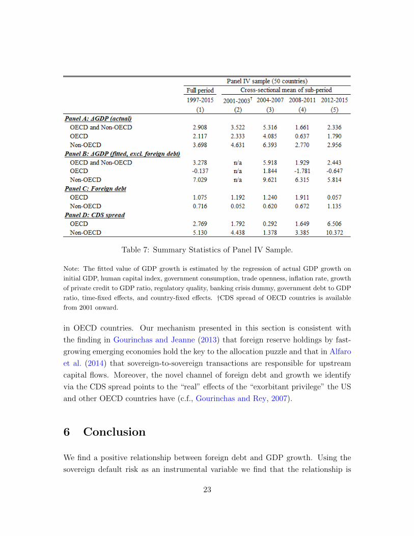
Table 7: Summary Statistics of Panel IV Sample.
Note: The fitted value of GDP growth is estimated by the regression of actual GDP growth on
initial GDP, human capital index, government consumption, trade openness, inflation rate, growth
of private credit to GDP ratio, regulatory quality, banking crisis dummy, government debt to GDP
ratio, time-fixed effects, and country-fixed effects. †CDS spread of OECD countries is available
from 2001 onward.
in OECD countries. Our mechanism presented in this section is consistent with
the finding in Gourinchas and Jeanne (2013) that foreign reserve holdings by fast-
growing emerging economies hold the key to the allocation puzzle and that in Alfaro
et al. (2014) that sovereign-to-sovereign transactions are responsible for upstream
capital flows. Moreover, the novel channel of foreign debt and growth we identify
via the CDS spread points to the “real” effects of the “exorbitant privilege” the US
and other OECD countries have (c.f., Gourinchas and Rey, 2007).
6 Conclusion
We find a positive relationship between foreign debt and GDP growth. Using the
sovereign default risk as an instrumental variable we find that the relationship is
23

causal in nature. Moreover, using a local projection analysis we find that an in-
crease in foreign debt leads to an increase in investment and then GDP growth in
subsequent years. On average, the sovereign default risk is lower and foreign debt
is higher in OECD than non-OECD countries. This suggests that sovereign default
risks are responsible for upstream capital flows that contribute to GDP growth in
OECD countries. Foreign debt accounts partially for growth not explained by stan-
dard controls in OECD countries. More comprehensive data that decompose the
debt instrument in portfolio investment by the type of issuers (public vs private)
would allow us identify the exact channel how foreign debt increases investment.
24
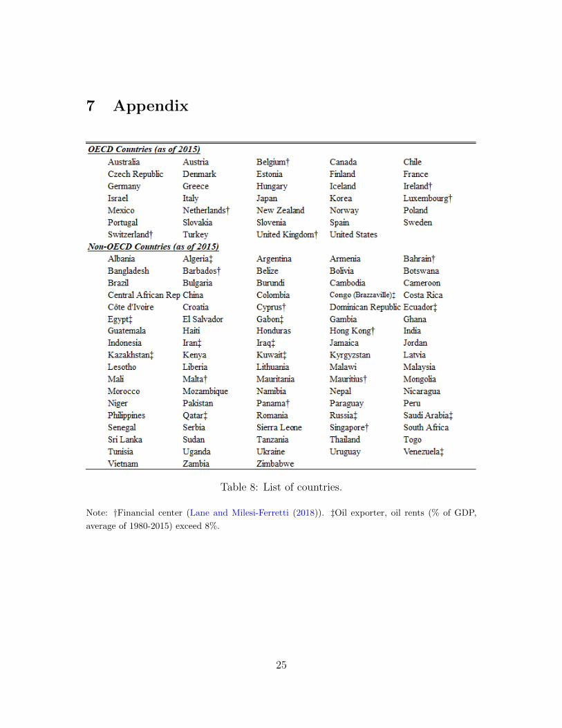
7 Appendix
Table 8: List of countries.
Note: †Financial center (Lane and Milesi-Ferretti (2018)). ‡Oil exporter, oil rents (% of GDP,
average of 1980-2015) exceed 8%.
25

Table 9: Ranking of Oil Rents (% of GDP)
Note: ‡Oil exporter. Oil rents are the difference between the value of crude oil production
at world prices and total costs of production
26

Table 10: Additional specification.
Note: The dependent variable is real GDP growth. The endogenous or independent variable is
foreign debt (the debt instrument of portfolio investment divided by GDP) instrumented with
sovereign CDS spread. Control variables are the lag of human capital index, government consump-
tion to GDP ratio (logged), trade openness (logged), inflation rate, initial level of GDP per capita
(logged), banking crisis dummy, general government gross debt to GDP ratio (logged), regulatory
quality, and growth of private credit to GDP ratio. Standard errors in parenthesis are clustered
on country. *** p<0.01, ** p<0.05, * p<0.1
27

Table 11: Comparison of predictive power.
Note: This table reports within R2. The dependent variable is real GDP growth, total investment
growth, private investment growth, or public investment growth. The independent variable is
foreign debt (the debt instrument of portfolio investment divided by GDP). Control variables are
the lag of initial GDP, human capital index, government consumption, trade openness, inflation
rate, growth of private credit to GDP ratio, regulatory quality, banking crisis dummy, government
debt to GDP ratio, time-fixed effects, and country-fixed effects.
28
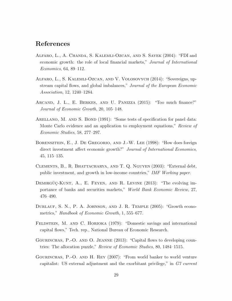
References
Alfaro, L., A. Chanda, S. Kalemli-Ozcan, and S. Sayek (2004): “FDI and
economic growth: the role of local financial markets,” Journal of International
Economics, 64, 89–112.
Alfaro, L., S. Kalemli-Ozcan, and V. Volosovych (2014): “Sovereigns, up-
stream capital flows, and global imbalances,” Journal of the European Economic
Association, 12, 1240–1284.
Arcand, J. L., E. Berkes, and U. Panizza (2015): “Too much finance?”
Journal of Economic Growth, 20, 105–148.
Arellano, M. and S. Bond (1991): “Some tests of specification for panel data:
Monte Carlo evidence and an application to employment equations,” Review of
Economic Studies, 58, 277–297.
Borensztein, E., J. De Gregorio, and J.-W. Lee (1998): “How does foreign
direct investment affect economic growth?” Journal of International Economics,
45, 115–135.
Clements, B., R. Bhattacharya, and T. Q. Nguyen (2003): “External debt,
public investment, and growth in low-income countries,” IMF Working paper.
Demirguc-Kunt, A., E. Feyen, and R. Levine (2013): “The evolving im-
portance of banks and securities markets,” World Bank Economic Review, 27,
476–490.
Durlauf, S. N., P. A. Johnson, and J. R. Temple (2005): “Growth econo-
metrics,” Handbook of Economic Growth, 1, 555–677.
Feldstein, M. and C. Horioka (1979): “Domestic savings and international
capital flows,” Tech. rep., National Bureau of Economic Research.
Gourinchas, P.-O. and O. Jeanne (2013): “Capital flows to developing coun-
tries: The allocation puzzle,” Review of Economic Studies, 80, 1484–1515.
Gourinchas, P.-O. and H. Rey (2007): “From world banker to world venture
capitalist: US external adjustment and the exorbitant privilege,” in G7 current
29

account imbalances: sustainability and adjustment, University of Chicago Press,
11–66.
Jorda, O. (2005): “Estimation and inference of impulse responses by local projec-
tions,” American Economic Review, 95, 161–182.
Kaufmann, D., A. Kraay, and M. Mastruzzi (2011): “The Worldwide Gov-
ernance Indicators: Methodology and Analytical Issues1,” Hague Journal on the
Rule of Law, 3, 220–246.
Kikuchi, T. and J. Stachurski (2009): “Endogenous inequality and fluctuations
in a two-country model,” Journal of Economic Theory, 144, 1560–1571.
Kikuchi, T., J. Stachurski, and G. Vachadze (2018): “Volatile capital flows
and financial integration: The role of moral hazard,” Journal of Economic Theory,
176, 170–192.
Kose, M. A., S. Kurlat, F. Ohnsorge, and N. Sugawara (2017): A cross-
country database of fiscal space, The World Bank.
Krugman, P. (1988): “Financing vs. forgiving a debt overhang,” Journal of De-
velopment Economics, 29, 253–268.
Laeven, L. and F. Valencia (2013): “Systemic banking crises database,” IMF
Economic Review, 61, 225–270.
——— (2020): “Systemic banking crises database II,” IMF Economic Review, 1–55.
Lane, P. R. and G. M. Milesi-Ferretti (2018): “The external wealth of
nations revisited: international financial integration in the aftermath of the global
financial crisis,” IMF Economic Review, 66, 189–222.
Lucas, R. E. (1990): “Why doesn’t capital flow from rich to poor countries?”
American Economic Review, 80, 92–96.
Matsuyama, K. (2004): “Financial market globalization, symmetry-breaking, and
endogenous inequality of nations,” Econometrica, 72, 853–884.
30

Mendoza, E. G., V. Quadrini, and J.-V. Rios-Rull (2009): “Financial inte-
gration, financial development, and global imbalances,” Journal of Political econ-
omy, 117, 371–416.
Pattillo, C. A., H. Poirson, and L. A. Ricci (2002): “External debt and
growth,” IMF Working Paper.
Reinhart, C. M., V. R. Reinhart, and K. S. Rogoff (2012): “Public debt
overhangs: advanced-economy episodes since 1800,” Journal of Economic Per-
spectives, 26, 69–86.
Reinhart, C. M. and K. S. Rogoff (2010): “Growth in a Time of Debt,”
American Economic Review, 100, 573–78.
31