does comparative advantage explain countries'...
TRANSCRIPT
1
Does comparative advantage explain countries' diversification level?
Asier Minondo
Deusto Business School Camino de Mundaiz, 50; 20012 San Sebastián (Spain)
Tel.: +34 943 326600; Fax: +34 943 273932 E-mail: [email protected]
Abstract
This paper analyses whether the products in which a country has comparative advantage can explain its exports' diversification level. We argue that specialisation endows countries with some specific skills and assets; in some cases those skills and assets can easily be redeployed in other products and facilitate diversification, whereas in other cases skills and assets are more difficult to redeploy and offer scant diversification possibilities. Based on countries' comparative advantage and an index of product proximity developed by Hidalgo et. al (2007), we construct a metric for countries diversification possibilities. Using non-parametric and parametric techniques, we show that this metric is a very strong and robust predictor of countries' actual diversification level, even when we control for differences in income across countries. These results point out that diversification may not be an automatic outcome of development. JEL Code: F10 Keywords: product proximity, export diversification, international trade, comparative advantage
Acknowledgements: I am grateful to Cesar Hidalgo and two anonymous referees for many helpful suggestions. Any errors or omissions remain the author's own responsibility.
2
1. Introduction
Export diversification has recently become a hot topic in the economic research agenda
(Carrère, Strauss-Kahn and Cadot, 2009; Newfarmer, Shaw and Walkenhorst, 2009). There
are old and new reasons that may explain this interest in export diversification. On the one
hand, diversification is considered a key policy objective for countries specialised in natural
resources (Sachs and Warner, 2001). On the other hand, countries seeking to accelerate
economic growth through exports should determine whether diversification, rather than the
intensive margin, is the best route to achieve this goal (Besedes and Prusa, 2007). In addition
to that, some models suggest that countries can increase their growth rate if they diversify into
products where learning by doing is larger (Matsuyama, 1992) or into rich-country products
(Hausmann, Hwang and Rodrik, 2007). In any case, other models warn that diversification
may be hampered due to the costs involved in discovering the new export products
(Hausmann and Rodrik, 2003).
If exports diversification has a positive effect on economic growth, a relevant question is what
determines its level. Some scholars show that diversification can be an outcome of the
development process. Imbs and Wacziarg (2003), Koren and Tenreyro (2007), Cadot, Carrère
and Strauss-Kahn (2009) and Klinger and Lederman (2009) find that countries grow through
two stages of diversification. At low levels of income growth is accompanied by an increase
in the level of diversification; however, once countries reach a certain level of income further
growth is accompanied by re-concentration. In contrast, Parteka and Tamberi (2008) and De
Benedictis, Gallegati and Tamberi (2009) conclude that growth is always accompanied by an
increase in the level of diversification.1
The contribution of this paper is to present and test an alternative explanation of the
differences in export diversification across countries. We argue that countries' diversification
levels may be determined by the products in which it has comparative advantage. The link
between comparative advantage and diversification is established through the concept of
product proximity developed by Hidalgo et al. (2007). These authors show that some
products, such as electronics, tend to be exported along with a large range of different
products; in contrast, other commodities, such as oil, tend to be exported alone. According to
1 It is important to indicate that there are differences across studies with respect to the diversification index used and its absolute or relative nature.

3
these authors, those differences are related to the skills and other assets, such as technology,
capital or institutions, needed to produce each product. For example, the manufacturing of
electronic products demand skills and assets that can easily be deployed in a large range of
additional manufactures (e.g. to master the logistics of the components that are assembled in a
factory); however, the extraction of oil demands skills and assets that are more difficult to
redeploy in other products (e.g. to master the operation of a drilling rig). Due to these
differences, countries that happen to develop comparative advantage in products that are close
to other products can diversify more easily than countries that happen to develop comparative
advantage in products that are in the periphery of the product space.
To test the validity of this explanation, we build an index of countries' diversification
possibilities based on the products in which they have comparative advantage and the
proximity of those products to the rest of commodities. Using non-parametric and parametric
techniques, we show that this index is a very strong and robust predictor of countries' actual
diversification levels, even when we control for differences in GDP per capita across
countries. These results point out that countries' diversification levels might not be an
automatic outcome of countries' development process. The conclusions of our paper are in
line with a recent study by Hidalgo and Hausmann (2009), who using network techniques
show that countries that have comparative advantage in products in which few countries also
have comparative advantage are endowed with a larger set of capabilities; this larger set of
capabilities, in turn, allows countries to export a larger set of products.
The rest of the paper is organised as follows. Section 2 explains in detail the relationship
between countries' comparative advantage and their exports diversification level. Section 3
presents the empirical analyses and Section 4 concludes.
2. The link between comparative advantage and diversification
To establish the link between the products in which a country has comparative advantage and
the diversification level we draw on the concept of product proximity developed by Hidalgo
et al. (2007). These authors argue that several dimensions may influence the degree of
relatedness between two products: similarities in the combination of productive factors, the
characteristics of the technology used in production, the use of a specific component, the

4
features of the final customers or the use of specific distribution channels. Due to the myriad
of factors that may determine the relatedness between products, they use an outcome measure
to calculate the degree of proximity between products. They argue that two products will be
close to each other if countries tend to have revealed comparative advantage in both products.
Based on this idea they calculate proximity (ϕ) between product i and product j at year t as:
{ })|(),|(min ,,,, titjtjtiijt xxPxxP=ϕ (1)
where P(xi,t | xj,t) is the conditional probability of having revealed comparative advantage in
product i given that the country has revealed comparative advantage in product j.
Based on this index and using network displaying techniques Hidalgo et al. (2007) are able to
draw a product space map. This map shows that products are not evenly distributed: there are
sections of the map with a high density of products, whereas other sections of the map are
sparsely populated. Our argument is that these discontinuities in the product map are very
important to determine countries' diversification opportunities. If a country happens to
develop comparative advantage in a product which is close to a large number of other
commodities, it will be easier for this country to diversify into new products. In contrast, if a
country happens to develop comparative advantage in a very sparsely populated zone of the
map, its diversification opportunities will be more scant. Hidalgo et al. (2007) provide
evidence that diversification is governed by the relatedness between products. They show that
countries tend to develop comparative advantage in those goods that are close to the products
in which they have comparative advantage. According to this model, changes in a country's
comparative advantage will lead to alterations in its diversification possibilities and, hence, on
its exports diversification level.
The concept of product proximity can be rephrased in the framework of cones of
diversification developed by Schott (2003) and Xian (2007). These authors argue that as
countries accumulate capital (and other productive factors) they move to new diversification
cones. In these models countries also shift from a product to a nearby product; however, in
this case the closeness between products is determined by how they combine the productive
factors in the production process. In Hidalgo et al. (2007) the proximity index encompasses
not only the similarity in the ratio in which factors of production are combined, but also other

5
features that may influence the relatedness between products. In addition to that, Hidalgo et
al. (2007) argue that some cones of diversification may encompass a larger number of goods
than others. Countries that end-up in diversification cones that cover a larger number of goods
will be able to diversify into more products than countries that end-up in diversification cones
with a smaller number of goods.2
To construct a metric for a country's diversification possibilities, we first, following
Hausmann and Klinger (2007), calculate an index of product centrality, which is defined as
the average proximity of a product to the rest of products:
JCentrality j
ijt
it
∑=
ϕ (2)
where J is the total amount of products. Second, based on this index, we calculate a country's
diversification possibilities as the average centrality of products in which the country has
revealed comparative advantage.
3. Empirical analyses
Data
We use data from the NBER World Trade Database to calculate product proximity indexes
(Feenstra et al., 2005). This database offers data for SITC Rev. 2, 4-digit classification, that
distinguishes 775 products. Countries diversification possibilities are calculated for the 1980-
2000 period. As we need to calculate countries' revealed comparative advantage to get
countries' diversification possibilities, the sample of countries should be the same for the
whole period. There are 91 countries that meet that criteria.3 Based on the same sample,
product proximity indexes are calculated at the beginning of the period: 1980. To avoid
reverse causality, we calculate a product proximity index set for each country. A country's
2 As Cadot, Carrère and Strauss-Kahn (2009) point out, the diversification level may increase, temporarily, even when a country moves to a new diversification cone that encompasses the same number of goods. This may occur if incumbency advantages make the phasing-out of old products slower than the addition of new products to the export basket. 3 We exclude from the sample countries with a population of less than 3 million.

6
product proximity index set is calculated by removing that country from the sample that is
used to calculate product proximity indexes. Data on countries GDP per capita in constant
PPP are obtained from the World Bank's World Development Indicators.
Exports diversification index
Following Cadot, Carrère and Strauss-Kahn (2009), the diversification of a country's export
structure is calculated using a Theil index:4
⎟⎟⎠
⎞⎜⎜⎝
⎛= ∑
= µµi
J
i
i xxJ
T ln11
where J
xJ
ii∑
== 1µ
where J is the total number of products and xi denotes the amount of exports of product i. The
Theil index is inversely related with a country's diversification level: the larger the index the
lower the diversification level. In addition to the Theil index, in the parametric estimations, to
asses the robustness of our results, we also use other concentration indexes, such as the
Herfindahl index and the Gini coefficient.
Non-parametric estimations
In the first set of estimations we use non-parametric techniques to analyse the relationship
between our relevant variables: diversification, countries' centrality and GDP per capita. The
advantage of non-parametric estimations is that they do not impose any prior functional form
on the estimated relationship. For our analyses we use a lowess smoothing function.
First, as in previous studies, we analyse the relationship between GDP per capita and
diversification.5 Figure 1 presents the relationship between GDP per capita and the Theil
index. As shown in the figure, we observe that the relationship between GDP per capita and
concentration follows a convex curve: there is sharp reduction in concentration when GDP
per capita rises from low income levels, but the slope becomes smoother when larger GDP
per capita levels are reached. The lowest concentration level happens at around 24000 PPP $,
similar to the turning-point level found by Cádot, Carrère and Strauss-Kahn (2009). From this 4 The Theil index is derived from Shannon's measure of information entropy. 5 Due its very large PPP GDP per capita, United Arab Emirates behaves as an outlier and, hence, is excluded from the sample.
7
GDP per capita onward there is almost a flat relationship between income and diversification.
This result is not in line with the re-concentration process found by Imbs and Wacziarg
(2003), Koren and Tenreyro (2007), Klinger and Lederman (2009) and Cádot, Carrère and
Strauss-Kahn (2009); however, it is in line with the results in Parteka and Tamberi (2008) and
De Benedictis, Gallegati and Tamberi (2009) who do not find either a two-stage process.6
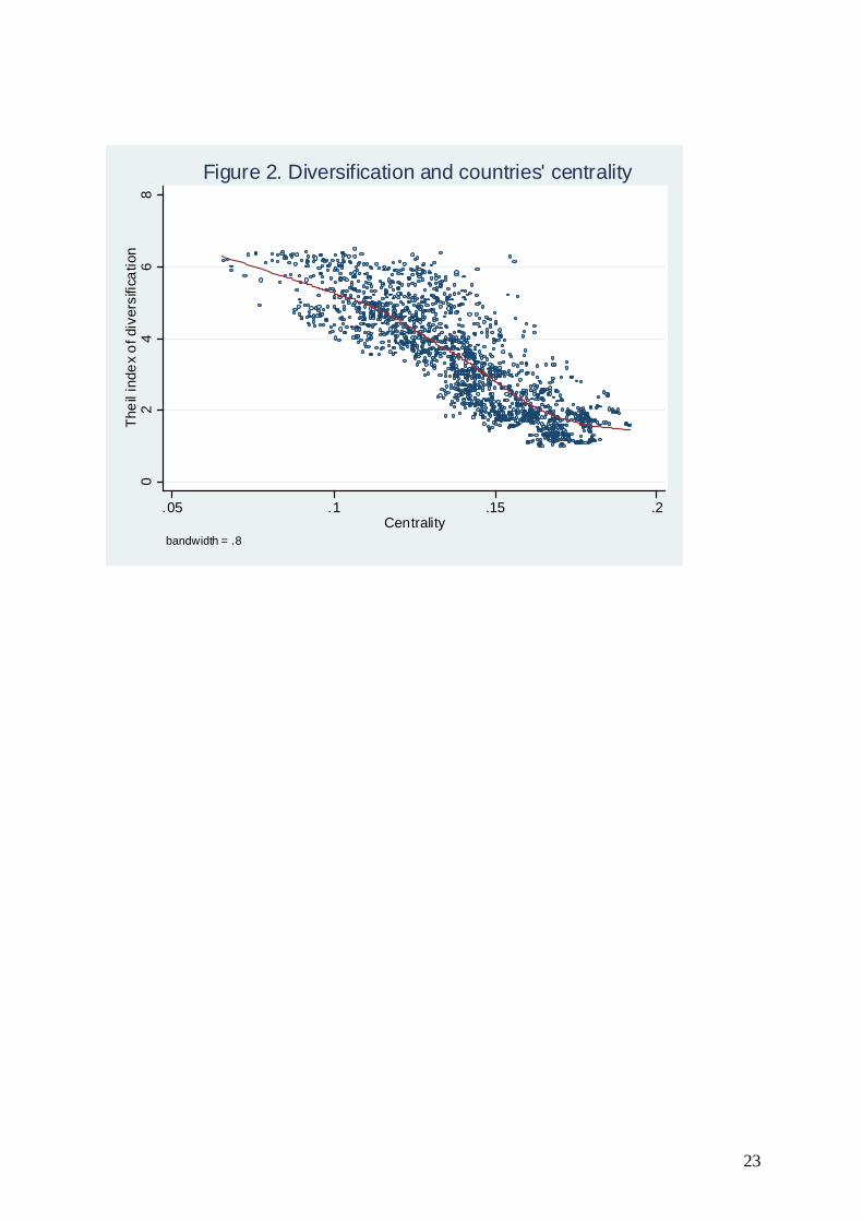
Figure 2 presents the relationship between our index of countries' diversification possibilities,
countries' centrality, and the Theil index. As expected, we find that countries with a larger
centrality index have a lower concentration level. This result confirms that countries with
revealed comparative advantage in goods that are close to a large number of other
commodities are able to export a larger range of goods than countries that have revealed
comparative advantage in goods that are in the periphery of the product space. To analyse
whether the positive relationship between countries' centrality and diversification is governed
by GDP per capita, Figure 3 presents the relationship between GDP per capita and centrality.
We can observe that there is, in fact, a positive relationship between both variables. However,
we can also see that there are large differences in the level of countries' centrality for the same
GDP per capita level. To sum up, non-parametric analyses show that both GDP per capita
and centrality may explain countries' diversification levels. Hence, to determine what is the
relative contribution of both variables to countries' diversification the next section presents the
results of parametric estimations.
Parametric estimations
Table 1 and Table 2 present the results of the parametric estimations. In Table 1, following
the re-concentration hypothesis, we assume a non-monotonic and non-linear relationship
between diversification and GDP per capita. In order to capture this non-monotonic and non-
linear relationship, following previous studies, we introduce GDP per capita and the square of
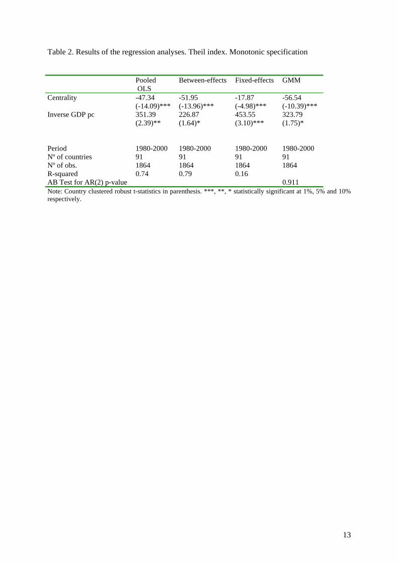
GDP per capita as independent variables. In Table 2, we assume that there is a monotonic
relationship between diversification and GDP per capita. In order to capture this monotonic
relationship we introduce the inverse of the GDP per capita as independent variable. This
functional form is non-linear, as in the previous case; however, contrary to the previous
functional form, it is monotonic. For each specification, we estimate four different models.
6 To analyse whether the differences in results were driven by the non-parametric technique used in the analyses, following these later authors, we also estimated a generalized additive regression model (GAM), with no changes in the shape of the fitted curves.

8
First, we pool all observations and estimate the model with simple OLS. Taking advantage of
the panel structure of our dataset, second, we estimate a between-effects model; third, a fixed-
effects model and fourth, to control for the possible endogeneity between the dependent and
independent variables, a GMM model.7 Finally, we estimate all the models with centrality as
the only independent variable and, then, we introduce the GDP per capita coefficient, in its
non-monotonic and monotonic specification, as an additional independent variable.
As there is much more variation in diversification across countries than within countries, the
pooled OLS and the between-effects models have a much larger R-square than the fixed-
effects model. We can observe that both in the non-monotonic (Table 1) and in the monotonic
specification (Table 2), centrality has a negative and statistically significant coefficient in all
models. These results point out that countries' diversification possibilities play a very strong
role in determining countries' exports diversity. We can see, as well, that centrality has a
negative coefficient and it is statistically significant even when we control for differences in
GDP per capita across countries. In Table 1, we observe that GDP per capita has a negative
coefficient and the square of GDP per capita has a positive coefficient, confirming the
predictions of a non-monotonic relationship between income and diversification. However,
GDP per capita and the square of GDP per capita are only statistically significant in the fixed-
effects model. In the monotonic specification, the inverse of GDP per capita is always
positive and statistically significant. As explained above, to control for endogeneity, in the
last columns of Table 1 and Table 2 we estimate a GMM model. The (System) GMM model
treats all covariates as potentially endogenous and include their lags and first-differences as
instruments. We observe that in all specifications, centrality remains negative and statistically
significant. Moreover, in all GMM estimations, we cannot reject the crucial assumption of no
second-order correlation of the residuals.
To further analyse the robustness of our results we perform additional regressions analyses.
First, previous studies, such as Parteka and Tamberi (2008) and Starosta de Waldemar (2010),
show that country size influences countries' diversification possibilities.8 If economies of
scale are prevalent, smaller countries will have less opportunities to develop a large range of
industries. Table 3a and Table 3b in the Appendix present the results of the estimations when 7 We do not present the results for the random-effects model because the Hausmann test rejects the null hypothesis of no correlation between the independent variables and country random effects. 8 Other less time-variant variables that may also influence diversification possibilities, such as rent-seeking or geography, are control for in the fixed-effects model estimation.

9
we introduce a variable for country size. We use two variables to proxy country size: GDP
and population. As expected, both population and GDP coefficients are negative, confirming
that larger countries have more diversification opportunities than smaller countries; however,
the population coefficient is not statistically significant in the non-monotonic specification's
between-effects model and the GDP coefficient is only statistically significant in the
monotonic-specification's pooled OLS model. The centrality coefficient has the correct sign
and remains statistically significant in all estimations.
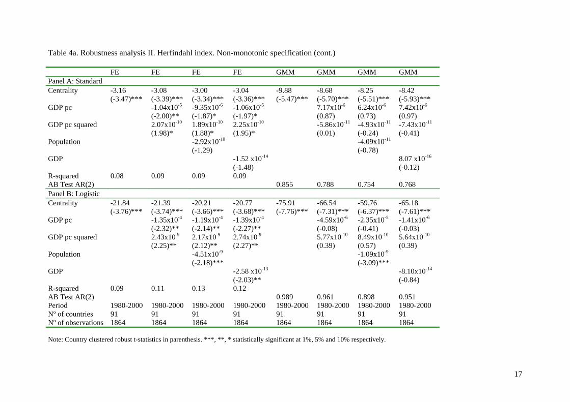
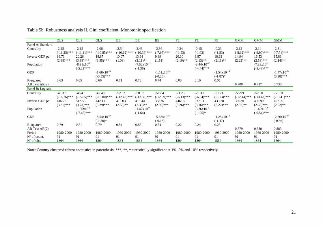
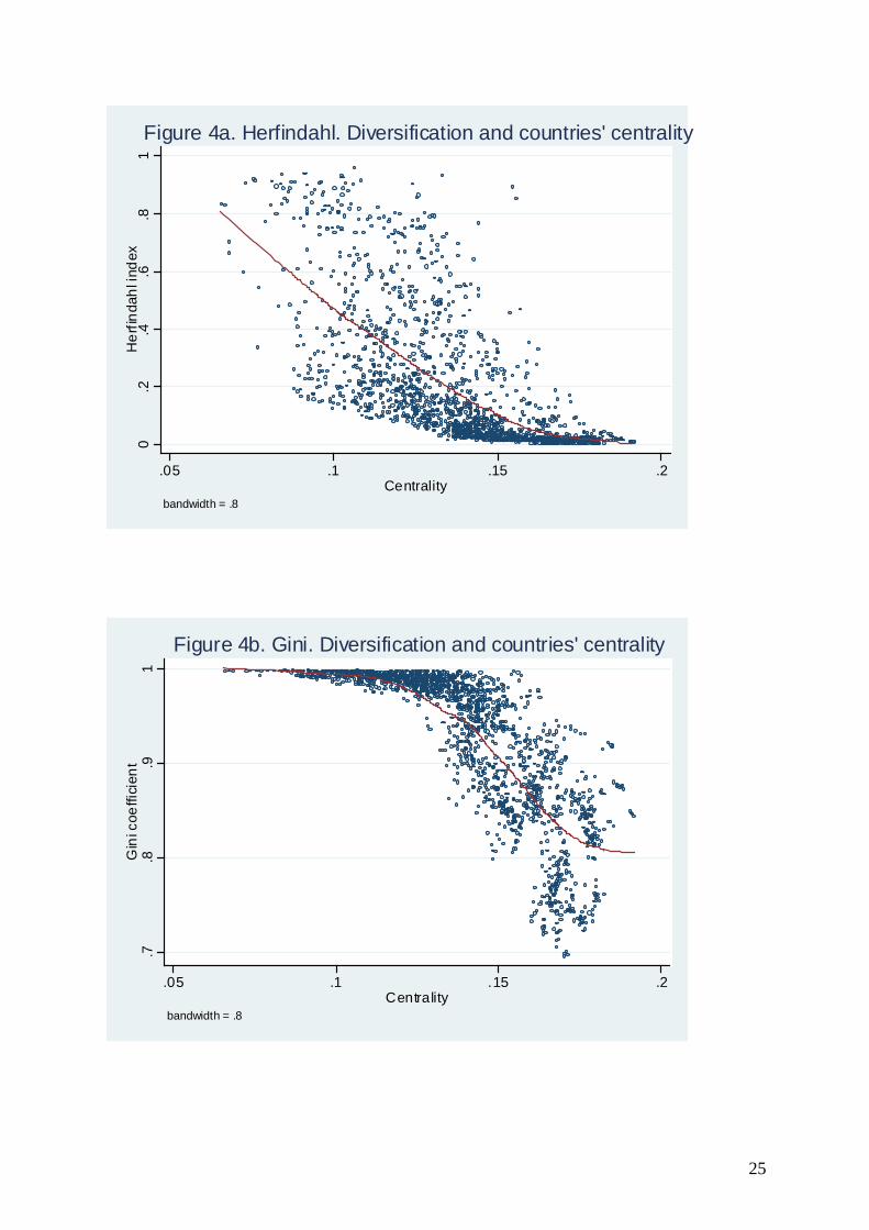
Second, we perform the econometric analyses using alternative measures for export
concentration: the Herfindahl index and the Gini coefficient. One limitation of these indexes
is that they are bounded between zero and one. Moreover, as shown in Figures 4a and 4b, in
our sample countries Herfindahl indexes are clustered around zero and Gini coefficients are
clustered around one. As the censoring of data may lead to biased estimations, following
Cádot, Carrère and Strauss-Kahn (2009), we also estimate the models using a logistic
transformation of the Herfindahl and Gini coefficients. In the case of the Herfindahl index
(Tables 4a and 4b in the Appendix), centrality has always a negative coefficient and is
statistically significant. We can observe that estimations with the logistic transformation
(Panel B) yield better results than estimations with the standard coefficient. First, the fit of the
model is always larger with the logistic transformation, specially in the non-monotonic
specification. Second, in the non-monotonic specification the logistic transformation yield the
expected coefficients on GDP per capita and the square of GDP per capita in all estimations.
When the Gini coefficient is used as the dependent variable, the centrality index has the
correct sign in all estimations. However, it is statistically not significant in five of the seven
estimations of the fixed-effects model with the standard coefficient (Table 5a and Table 5b in
the Appendix - Panel A). This results might be explained by the large degree of observations
that are clustered around the value 1 (Figure 4b). In fact, when we estimate the fixed-effects
model with the logistic transformation the centrality coefficient is always negative and
statistically significant.
10
4. Conclusions
In this paper we show that the products in which a country has comparative advantage may
play a very important role on countries' exports diversification level. We argue that countries
that develop comparative advantage in commodities that demand skills and assets that can be
easily redeploy in other products have more opportunities to diversify into new products than
countries that develop comparative advantage in goods that demand skills and assets that are
more difficult to redeploy. To test this hypothesis we calculate an index of countries
diversification possibilities that combines countries' comparative advantage and proximity
between products. Using non-parametric and parametric techniques we show that the
diversification possibilities index is a strong predictor of countries actual diversification level,
even when we control for differences in GDP per capita across countries. These results
indicate that the products in which a country has comparative advantage play a very important
role in explaining the level of export diversification; hence, export diversification might not
be an automatic outcome of the process of development.
References Besedes, T. and Prusa, T.J. (2007). “The Role of Extensive and Intensive Margins and Export Growth", NBER Working Paper 13268, National Bureau of Economic Research, Cambridge, MA. Cadot, O., Carrèrre, C. and Strauss-Kahn, V. (2009). "Export Diversification: What's Behind the Hump", CEPR Discussion Paper Series Nº 6590. Carrèrre, C., Strauss-Kahn, V. and Cadot, O. (2009). "Trade Diversification, Income and Growth: What Do We Know?", CERDI Working Paper E 2009.31 De Benedictis, L., Gallegati, L. and Tamberi, M. (2009). "Overall trade specialization and economic development: countries diversify", Review of World Economics, 145, 1, 37-55. Feenstra, R.C., Lipsey, R.E., Deng, H. Ma, A.C. y Mo, H. (2005). "World Trade Flows: 1962-2000", NBER Working Paper 11040, National Bureau of Economic Research, Cambridge, Massachusets. Hausmann, R. and Klinger, B. (2007): “The Structure of the Product Space and the Evolution of Comparative Advantage”, CID Working Paper No. 146 Hausmann, R., Hwang, J, and Rodrik, D. (2007). "What You Export Matters", Journal of Economic Growth, 12, 1, 1-25.
11
Hausmann, R. and Rodrik, D. (2003). "Economic development as self discovery", Journal of Development Economics, 72, 2, 602-633. Hidalgo, C.A. and Hausmann, R. (2009). "The building blocks of economic complexity", Proceedings of the National Academy of Sciences, 106, 26, 10570-10575. Hidalgo, C.A., Klinger, B., Barabási, A.L. y Hausmann, R. (2007). "The Product Space Conditions the Development of Nations", Science, 317, 5837, 482-487. Imbs, J. and Wacziarg, R. (2003). "Stages of Diversification", American Economic Review, 93, 1, 63-86. Klinger, B. and Lederman, D. (2009). "Diversification, Innovation, and Imitation of the Global Technological Frontier", in Newfarmer, R., Shaw, W. and Walkenhorst, P. (eds.) Breaking into New Markets. Emerging Lessons for Export Diversification, The World Bank, Washington D.C. Koren, M. and Tenreyro, S. (2007). "Volatility and Development", Quarterly Journal of Economics, 122, 1, 243-287. Matsuyama, K. (1992). "Agricultural Productivity, Comparative Advantage and Economic Growth", Journal of Economic Theory, 58, 2, 317-334. Newfarmer, R., Shaw, W. and Walkenhorst, P. (eds.) (2009). Breaking into New Markets. Emerging Lessons for Export Diversification, The World Bank, Washington D.C. Parteka, A. and Tamberi, M. (2008). "Determinants of Export Diversification: An Empirical Investigation", Quaderni di Ricerca nº 327, Università Politecnica delle Marche Sachs, J.D. and Warner. A.M. (2001). “The curse of natural resources”, European Economic Review, 45, 4-6, 827-838. Schott, P. K. (2003). "One Size Fits All? Heckscher-Ohlin Specialization in Global Production", American Economic Review, 93, 3, 686-708. Starosta de Waldemar, F. (2010). "How costly is rent-seeking to diversification: an empirical approach", CES Working Papers 2010.08. Xiang, C. (2007). "Diversification cones, trade costs and factor market linkages", Journal of International Economics, 71, 2, 448-466

12
Table 1. Results of the regression analyses. Theil index. Non-monotonic specification Pooled
OLS Pooled OLS
Between-effects Between-effects Fixed-effects Fixed- effects
GMM GMM
Centrality -52.32 (-21.84)***
-46.16 (-9.29)***
-55.46 (-24.18)***
-52.72 (-8.46)***
-17.83 (-4.42)***
-17.75 (-4.54)***
-62.62 (-9.43)***
-53.89 (-8.01)***
GDP pc -5.31x10⁻⁵
(-1.45) -3.79x10⁻⁵
(-0.74) -1.38x10⁻⁴
(-3.04)*** -3.59x10⁻⁵
(-0.84) GDP pc squared 1.23x10⁻⁹
(1.27) 1.26x10⁻⁹
(0.82) 2.30x10⁻⁹
(2.73)*** 1.03x10⁻⁹
(0.96) Period 1980-2000 1980-2000 1980-2000 1980-2000 1980-2000 1980-2000 1980-2000 1980-2000 Nº of countries 91 91 91 91 91 91 91 91 Nº of observations. 1864 1864 1864 1864 1864 1864 1864 1864 R-squared 0.72 0.77 0.79 0.80 0.12 0.18 AB Test for AR(2) p-value 0.851 0.854 Note: Country clustered robust t-statistics in parenthesis. ***, **, * statistically significant at 1%, 5% and 10% respectively.
13
Table 2. Results of the regression analyses. Theil index. Monotonic specification Pooled
OLS Between-effects Fixed-effects GMM
Centrality -47.34 (-14.09)***
-51.95 (-13.96)***
-17.87 (-4.98)***
-56.54 (-10.39)***
Inverse GDP pc 351.39
(2.39)** 226.87
(1.64)* 453.55
(3.10)*** 323.79 (1.75)*
Period 1980-2000 1980-2000 1980-2000 1980-2000 Nº of countries 91 91 91 91 Nº of obs. 1864 1864 1864 1864 R-squared 0.74 0.79 0.16 AB Test for AR(2) p-value 0.911 Note: Country clustered robust t-statistics in parenthesis. ***, **, * statistically significant at 1%, 5% and 10% respectively.

14
Appendix Table 3a. Robustness analysis I. Countries size included as independent variable. Non-monotonic specification Pooled
OLS Between- effects
Fixed- effects
GMM Pooled OLS
Between- effects
Fixed- effects
GMM
Centrality -41.85 (-7.96)***
-49.22 (-9.25)***
-16.80 (-4.55)***
-48.38 (-7.01)***
-45.65 (-9.18)***
-53.16 (-8.45)***
-17.48 (-4.50)***
-54.19 (-8.59)***
GDP pc -8.11x10⁻⁵
(-2.19)** -6.67x10⁻⁵
(-1.53) -1.25x10⁻⁴
(-2.90)*** -5.22x10⁻⁵
(-1.20) -5.73x10⁻⁵
(-1.59) -4.40x10⁻⁵
(-1.04) -1.39x10⁻⁴
(-2.98)*** -2.68x10⁻⁵
(-0.67) GDP pc squared 1.87x10⁻⁹
(1.98)** 1.94x10⁻⁹ (1.50)
2.09x10⁻⁹ (2.62)***
1.27x10⁻⁹ (1.19)
1.47x10⁻⁹ (1.56)
1.58x10⁻⁹ (1.26)
2.43x10⁻⁹ (2.65)***
8.70x10⁻¹⁰ (0.85)
Population -1.63x10⁻⁹ (-6.40)***
-1.41x10⁻⁹ (-1.43)
-3.57x10⁻⁹ (-2.33)**
-1.44x10⁻⁹ (-5.11)***
GDP -9.08x10⁻¹⁴ (-1.54)
-9.61x10⁻¹⁴
(-0.24) -1.08x10⁻¹³
(-1.52) -1.08x10⁻¹³
(-1.52) Period 1980-2000 1980-2000 1980-2000 1980-2000 1980-2000 1980-2000 1980-2000 1980-2000 Nº of countries 91 91 91 91 91 91 91 91 Nº of obs. 1864 1864 1864 1864 1864 1864 1864 1864 R-squared 0.76 0.82 0.20 0.74 0.80 0.18 AB Test for AR(2) p-value 0.873 0.852 Note: Country clustered robust t-statistics in parenthesis. ***, **, * statistically significant at 1%, 5% and 10% respectively.

15
Table 3b. Robustness analysis I. Countries size included as independent variable. Monotonic specification Pooled
OLS Between- effects
Fixed- effects
GMM Pooled OLS
Between- effects
Fixed- effects
GMM
Centrality -45.54 (-13.46)***
-49.98 (-13.39)***
-17.01 (-4.90)***
-52.63 (-11.08)***
-46.50 (-13.74)***
-51.35 (-11.58)***
-17.83 (-4.97)***
-54.56 (-11.29)***
Inverse GDP pc 412.20
(2.75)*** 294.82
(1.95)* 344.98
(2.85)*** 311.13
(1.82)* 347.48 (2.37)**
226.24 (1.36)
440.35 (3.05)***
331.07 (1.83)*
Population -1.43x10⁻⁹ (-7.62)***
-1.32x10⁻⁹ (-2.02)**
-3.27x10⁻⁹ (-1.94)*
-1.35x10⁻⁹ (-6.52)***
GDP -8.11x10⁻¹⁴ (-1.77)*
-5.12x10⁻¹⁴
(-0.15) -1.30x10⁻¹³
(-1.44) -1.75x10⁻¹⁴
(-0.36) Period 1980-2000 1980-2000 1980-2000 1980-2000 1980-2000 1980-2000 1980-2000 1980-2000 Nº of countries 91 91 91 91 91 91 91 91 Nº of obs. 1864 1864 1864 1864 1864 1864 1864 1864 R-squared 0.76 0.82 0.17 0.74 0.80 0.16 AB Test for AR(2) p-value 0.919 0.917 Note: Country clustered robust t-statistics in parenthesis. ***, **, * statistically significant at 1%, 5% and 10% respectively.

16
Table 4a. Robustness analysis II. Herfindahl index. Non-monotonic specification OLS OLS OLS OLS BE BE BE BE Panel A: Standard Centrality -6.43
(-9.07)*** -7.34 (-6.14)***
-7.14 (-5.51)***
-7.33 (-6.09)***
-6.74 (-8.16)***
-8.55 (-5.45)***
-8.44 (-5.66)***
-8.55 (-5.93)***
GDP pc 2.52x10⁻⁶
(0.37) 1.22x10⁻⁶
(0.16) 2.44x10⁻⁶
(0.35) 5.95x10⁻⁶
(0.72) 5.22x10⁻⁶
(0.66) 5.87x10⁻⁶
(0.65) GDP pc squared 3.08x10⁻¹¹
(0.18) 6.08x10⁻¹¹ (0.33)
3.54x10⁻¹¹ (0.21)
1.15x10⁻¹² (0.01)
1.83x10⁻¹¹ (0.09)
5.59x10⁻¹² (0.02)
Population -7.56x10⁻¹¹ (-1.52)
-3.57x10⁻¹¹ (-0.26)
GDP
-1.76 x10⁻¹⁵ (-0.28)
-1.35 x10⁻¹⁵ (-0.10)
R-squared 0.46 0.47 0.48 0.47 0.55 0.55 0.55 0.55 Panel B: Logistic Centrality -57.55
(-15.01)*** -54.89 (-7.75)***
-51.35 (-6.68)***
-54.30 (-7.70)***
-60.90 (-14.27)***
-64.06 (-7.66)***
-60.73 (-5.96)***
-63.44 (-6.42)***
GDP pc -3.73x10⁻⁵
(-0.77) -6.03x10⁻⁵
(-1.18) -4.23x10⁻⁵
(-0.89) -1.60x10⁻⁵
(-0.24) -3.73x10⁻⁵
(-0.51) -2.27x10⁻⁵
(-0.37) GDP pc squared 1.10x10⁻⁹
(0.82) 1.63x10⁻⁹ (1.20)
1.38x10⁻⁹ (1.04)
1.03x10⁻⁹ (0.51)
1.54x10⁻⁹ (0.70)
1.38x10⁻⁹ (0.74)
Population -1.34x10⁻⁹ (-4.17)***
-1.08x10⁻⁹ (-1.58)
GDP
-1.07 x10⁻¹³ (-1.17)
-1.06 x10⁻¹⁷ (-0.28)
R-squared 0.63 0.63 0.65 0.64 0.71 0.71 0.72 0.72 Period 1980-2000 1980-2000 1980-2000 1980-2000 1980-2000 1980-2000 1980-2000 1980-2000 Nº of countries 91 91 91 91 91 91 91 91 Nº of observations 1864 1864 1864 1864 1864 1864 1864 1864 Note: Country clustered robust t-statistics in parenthesis. ***, **, * statistically significant at 1%, 5% and 10% respectively.
17
Table 4a. Robustness analysis II. Herfindahl index. Non-monotonic specification (cont.) FE FE FE FE GMM GMM GMM GMM Panel A: Standard Centrality -3.16
(-3.47)*** -3.08 (-3.39)***
-3.00 (-3.34)***
-3.04 (-3.36)***
-9.88 (-5.47)***
-8.68 (-5.70)***
-8.25 (-5.51)***
-8.42 (-5.93)***
GDP pc -1.04x10⁻⁵
(-2.00)** -9.35x10⁻⁶
(-1.87)* -1.06x10⁻⁵
(-1.97)* 7.17x10-6
(0.87) 6.24x10⁻⁶
(0.73) 7.42x10⁻⁶
(0.97) GDP pc squared 2.07x10⁻¹⁰
(1.98)* 1.89x10-10 (1.88)*
2.25x10-10 (1.95)*
-5.86x10⁻¹¹ (0.01)
-4.93x10⁻¹¹ (-0.24)
-7.43x10⁻¹¹ (-0.41)
Population -2.92x10⁻¹⁰ (-1.29)
-4.09x10⁻¹¹ (-0.78)
GDP
-1.52 x10⁻¹⁴ (-1.48)
8.07 x10⁻¹⁶ (-0.12)
R-squared 0.08 0.09 0.09 0.09 AB Test AR(2) 0.855 0.788 0.754 0.768 Panel B: Logistic Centrality -21.84
(-3.76)*** -21.39 (-3.74)***
-20.21 (-3.66)***
-20.77 (-3.68)***
-75.91 (-7.76)***
-66.54 (-7.31)***
-59.76 (-6.37)***
-65.18 (-7.61)***
GDP pc -1.35x10⁻⁴
(-2.32)** -1.19x10⁻⁴
(-2.14)** -1.39x10⁻⁴
(-2.27)** -4.59x10⁻⁶
(-0.08) -2.35x10⁻⁵
(-0.41) -1.41x10⁻⁶
(-0.03) GDP pc squared 2.43x10⁻⁹
(2.25)** 2.17x10⁻⁹ (2.12)**
2.74x10⁻⁹ (2.27)**
5.77x10⁻¹⁰ (0.39)
8.49x10⁻¹⁰ (0.57)
5.64x10⁻¹⁰ (0.39)
Population -4.51x10⁻⁹ (-2.18)***
-1.09x10⁻⁹ (-3.09)***
GDP
-2.58 x10⁻¹³ (-2.03)**
-8.10x10⁻¹⁴ (-0.84)
R-squared 0.09 0.11 0.13 0.12 AB Test AR(2) 0.989 0.961 0.898 0.951 Period 1980-2000 1980-2000 1980-2000 1980-2000 1980-2000 1980-2000 1980-2000 1980-2000 Nº of countries 91 91 91 91 91 91 91 91 Nº of observations 1864 1864 1864 1864 1864 1864 1864 1864 Note: Country clustered robust t-statistics in parenthesis. ***, **, * statistically significant at 1%, 5% and 10% respectively.

18
Table 4b. Robustness analysis II. Herfindahl index. Monotonic specification OLS OLS OLS BE BE BE FE FE FE GMM GMM GMM Panel A: Standard Centrality -6.01
(-6.02)*** -5.86 (-5.70)***
-6.10 (-5.96)***
-6.58 (-5.88)***
-6.43 (-5.10)***
-6.73 (-5.30)***
-3.16 (-3.78)***
-3.12 (-3.75)***
-3.16 (-3.78)***
-8.82 (-5.97)***
-7.55 (-5.54)***
-7.92 (-5.95)***
Inverse GDP pc 29.55
(0.91) 34.52
(0.91) 29.97
(0.82) 10.14
(0.31) 15.37
(0.39) 10.29
(0.24) 60.93
(2.00)** 55.53
(1.72)* 60.38
(1.97)* 32.33
(0.72)** 22.76
(0.53) 32.32
(0.76) Population -1.17x10⁻¹⁰
(-3.21)*** -1.02x10⁻¹⁰
(-0.60) -1.63x10⁻¹⁰
(-0.67) -1.15x10⁻¹⁰
(-2.84)***
GDP
8.74 x10⁻¹⁵ (1.49)
1.26x10⁻¹⁴ (0.58)
-5.37x10⁻¹⁵ (-0.75)
2.33x10⁻¹⁴ (2.15)**
R-squared 0.47 0.47 0.47 0.52 0.53 0.53 0.10 0.10 0.10 AB Test AR(2) 0.753 0.664 0.686 Panel B: Logistic Centrality -53.45
(-10.11)*** -51.87 (-9.52)***
-52.74 (-9.78)***
-58.84 (-9.10)***
-57.19 (-8.55)***
-58.08 (-9.34)***
-21.89 (-4.21)***
-20.86 (-4.07)***
-21.83 (-4.20)***
-67.12 (-8.37)***
-61.26 (-8.47)***
-62.25 (-8.71)***
Inverse GDP pc 289.80 (1.43)
343.28 (1.64)
286.51 (1.41)
133.17 (0.49)
190.19 (0.70)
131.80 (0.66)
531.19 (2.51)**
401.04 (2.03)**
510.92 (2.45)**
303.67 (1.17)
258.00 (1.06)
314.94 (1.26)
Population -1.26x10⁻⁹ (-5.41)***
-1.11x10⁻⁹ (-1.45)
-3.92x10⁻⁹ (-1.79)*
-1.19x10⁻⁹ (-4.78)***
GDP -6.83 x10⁻¹⁴ (-1.02)
-3.06x10⁻¹⁴ (-0.09)
-1.99x10⁻¹³ (-1.39)
-1.26x10⁻¹⁴ (0.16)
R-squared 0.64 0.65 0.64 0.71 0.72 0.71 0.11 0.12 0.12 AB Test AR(2) 0.913 0.869 0.871 Period 1980-2000 1980-2000 1980-2000 1980-2000 1980-2000 1980-2000 1980-2000 1980-2000 1980-2000 1980-2000 1980-2000 1980-2000 Nº of count. 91 91 91 91 91 91 91 91 91 91 91 91 Nº of obs. 1864 1864 1864 1864 1864 1864 1864 1864 1864 1864 1864 1864 Note: Country clustered robust t-statistics in parenthesis. ***, **, * statistically significant at 1%, 5% and 10% respectively.

19
Table 5a. Robustness analysis II. Gini coefficient. Non-monotonic specification OLS OLS OLS OLS BE BE BE BE Panel A: Standard Centrality -2.49
(-13.12)*** -1.52 (-5.76)***
-1.20 (-4.82)***
-1.45 (-5.82)***
-2.70 (-6.80)***
-1.85 (-6.80)***
-1.50 (-4.31)***
-1.78 (-6.56)***
GDP pc -4.73x10⁻⁶
(-2.17)** -6.77x10⁻⁶
(-3.38)*** -5.27x10⁻⁶
(-2.67)*** -3.90x10⁻⁶
(-1.68)* -6.12x10⁻⁶
(-2.32)** -4.67x10⁻⁶
(-1.76)* GDP pc squared 4.91x10⁻¹¹
(0.71) 9.65x10⁻¹¹ (1.57)
8.02x10⁻¹¹ (1.32)
4.37x10⁻¹¹ (0.50)
9.60x10⁻¹¹ (1.08)
8.35x10⁻¹¹ (0.83)
Population -1.19x10⁻¹⁰ (-8.51)***
-1.09x10⁻¹⁰ (-1.05)
GDP
-1.18x10⁻¹⁴ (-2.11)**
-1.21x10⁻¹⁴ (-0.28)
R-squared 0.62 0.70 0.75 0.71 0.71 0.75 0.79 0.77 Panel B: Logistic Centrality -54.69
(-24.82)*** -46.20 (-10.19)***
-41.39 (-9.15)***
-45.74 (-10.24)***
-57.78 (-23.06)***
-52.92 (-10.75)***
-47.68 (-8.98)***
-52.38 (-8.49)***
GDP pc -6.79x10⁻⁵
(-2.10)** -9.91x10⁻⁵
(-3.13)*** -7.18x10⁻⁵
(-2.24)** -5.82x10⁻⁵
(-1.81)* -9.18x10⁻⁵
(-2.56)*** -6.41x10⁻⁵
(-1.73)* GDP pc squared 1.48x10⁻⁹
(1.82)* 2.21x10-9 (2.82)***
1.70x10--9 (2.12)**
1.66x10⁻⁹ (1.95)*
2.44x10-9 (2.50)**
1.96x10⁻⁹ (1.94)**
Population -1.82x10⁻⁹ (-6.82)***
-1.65x10⁻⁹ (-2.32)**
GDP
-8.37x10⁻¹⁴ (-1.45)
-9.30x10⁻¹⁴ (-0.16)
R-squared 0.77 0.78 0.81 0.78 0.83 0.83 0.86 0.84 Period 1980-2000 1980-2000 1980-2000 1980-2000 1980-2000 1980-2000 1980-2000 1980-2000 Nº of countries 91 91 91 91 91 91 91 91 Nº of observations 1864 1864 1864 1864 1864 1864 1864 1864 Note: Country clustered robust t-statistics in parenthesis. ***, **, * statistically significant at 1%, 5% and 10% respectively.

20
Table 5a. Robustness analysis II. Gini coefficient. Non-monotonic specification (cont.) FE FE FE FE GMM GMM GMM GMM Panel A: Standard Centrality -0.24
(-1.46) -0.28 (-2.06)**
-0.20 (-1.64)
-0.26 (-1.95)*
-2.39 (-7.35)***
-1.99 (-5.72)***
-1.60 (-4.44)***
-2.06 (-5.99)***
GDP pc -1.06x10⁻⁵
(-3.69)*** -9.46x10⁻⁶
(-3.51)*** -1.07x10⁻⁵
(-3.67)*** -3.88x10⁻⁶
(-1.58) -5.01x10⁻⁶
(-2.08)** -3.36x10⁻⁶
(-1.49) GDP pc squared 1.54x10⁻¹⁰
(3.17)*** 1.36x10⁻¹⁰ (3.02)***
1.63x10⁻¹⁰ (3.13)***
4.44x10⁻¹¹ (0.60)
6.03x10⁻¹¹ (0.86)
4.58x10⁻¹¹ (0.68)
Population -3.03x10⁻¹⁰ (-4.65)***
-1.06x10⁻¹⁰ (-6.76)***
GDP
-7.86x10⁻¹⁵ (-1.26)
-1.03x10⁻¹⁴ (-1.85)*
R-squared 0.01 0.17 0.23 0.17 AB Test AR(2) 0.679 0.721 0.708 0.711 Panel B: Logistic Centrality -21.20
(-5.54)*** -21.45 (-5.66)***
-20.53 (-5.69)***
-21.31 (-5.66)***
-61.98 (-10.40)***
-51.61 (-8.86)***
-47.08 (-7.94)***
-52.79 (-9.39)***
GDP pc -1.34x10⁻⁴
(-3.30)*** -1.21x10⁻⁴
(-3.14)*** -1.35x10⁻⁴
(-3.23)*** -5.69x10⁻⁵
(-1.53) -7.22x10⁻⁵
(-1.95)* -4.72x10⁻⁵
(-1.34) GDP pc squared 2.09x10⁻⁹
(2.65)*** 1.89x10⁻⁹ (2.52)**
2.16x10⁻⁹ (2.51)**
1.38x10⁻⁹ (1.52)
1.62x10⁻⁹ (1.84)*
1.23x10-9 (1.43)
Population -3.49x10⁻⁹ (-2.36)**
-1.65x10⁻⁹ (-5.82)***
GDP
-5.71x10⁻¹⁴ (-0.77)
-6.62x10⁻¹⁴ (-1.15)
R-squared 0.19 0.25 0.13 0.12 AB Test AR(2) 0.817 0.783 0.788 0.794 Period 1980-2000 1980-2000 1980-2000 1980-2000 1980-2000 1980-2000 1980-2000 1980-2000 Nº of countries 91 91 91 91 91 91 91 91 Nº of observations 1864 1864 1864 1864 1864 1864 1864 1864 Note: Country clustered robust t-statistics in parenthesis. ***, **, * statistically significant at 1%, 5% and 10% respectively.
21
Table 5b. Robustness analysis II. Gini coefficient. Monotonic specification OLS OLS OLS BE BE BE FE FE FE GMM GMM GMM Panel A: Standard Centrality -2.25
(-11.25)*** -2.15 (-11.11)***
-2.08 (-10.85)***
-2.54 (-10.62)***
-2.43 (-10.36)***
-2.36 (-7.65)***
-0.24 (-1.53)
-0.15 (-1.03)
-0.23 (-1.53)
-2.12 (-8.12)***
-2.14 (-9.90)***
-2.31 (-7.71)***
Inverse GDP pc 16.73
(2.68)*** 20.26
(3.38)*** 18.87
(3.35)*** 10.07 (1.08)
13.94
(2.11)** 9.89
(1.51) 20.30
(2.10)** 8.87
(2.13)** 18.63
(2.11)** 14.94
(2.22)** 16.53
(2.58)*** 15.83
(2.14)** Population -8.31x10⁻¹¹
(-5.21)*** -7.52x10⁻¹¹
(-1.36) -3.44x10⁻¹⁰
(-4.44)*** -7.32x10⁻¹¹
(-5.43)***
GDP
-1.68x10⁻¹⁴ (-3.35)***
-1.51x10⁻¹⁴ (-0.26)
-1.54x10⁻¹⁴ (-1.87)*
-1.47x10⁻¹⁴ (3.28)***
R-squared 0.63 0.65 0.66 0.71 0.73 0.74 0.03 0.10 0.05 AB Test AR(2) 0.700 0.717 0.730 Panel B: Logistic Centrality -48.37
(-16.26)*** -46.41 (-15.85)***
-47.48 (-16.00)***
-52.53 (-12.48)***
-50.33 (-12.38)***
-51.84 (-12.99)***
-21.25 (-6.13)***
-20.39 (-6.04)***
-21.21 (-6.13)***
-55.99 (-12.44)***
-52.50 (-13.48)***
-55.10 (-13.41)***
Inverse GDP pc 446.23 (3.31)***
512.56 (3.73)***
442.11 (3.29)***
415.03 (2.50)**
415.44 (2.35)**
338.97 (2.89)***
446.05 (3.26)***
337.91 (3.16)***
433.38 (3.22)***
386.91 (2.37)**
400.90 (2.66)***
407.09 (2.52)**
Population -1.56x10⁻⁹ (-7.45)***
-1.47x10⁻⁹ (-1.64)
-3.26x10⁻⁹ (-1.95)*
-1.48x10⁻⁹ (-6.54)***
GDP -8.54x10⁻¹⁴ (-1.80)*
-5.85x10⁻¹⁴ (-0.13)
-1.25x10⁻¹³ (-1.47)
-2.66x10⁻¹⁴ (-0.56)
R-squared 0.79 0.81 0.79 0.84 0.86 0.84 0.22 0.24 0.23 AB Test AR(2) 0.879 0.880 0.883 Period 1980-2000 1980-2000 1980-2000 1980-2000 1980-2000 1980-2000 1980-2000 1980-2000 1980-2000 1980-2000 1980-2000 1980-2000 Nº of count. 91 91 91 91 91 91 91 91 91 91 91 91 Nº of obs. 1864 1864 1864 1864 1864 1864 1864 1864 1864 1864 1864 1864 Note: Country clustered robust t-statistics in parenthesis. ***, **, * statistically significant at 1%, 5% and 10% respectively.

22
02
46
8Th
eil i
ndex
of d
iver
sific
atio
n
0 10000 20000 30000 40000GDP per capita
bandwidth = .8
Figure 1. Diversification and GDP per capita
23
02
46
8Th
eil i
ndex
of d
iver
sific
atio
n
.05 .1 .15 .2Centrality
bandwidth = .8
Figure 2. Diversification and countries' centrality

24
.05
.1.1
5.2
Cen
tralit
y
0 10000 20000 30000 40000GDP per capita
bandwidth = .8
Figure 3. Countries' centrality and GDP per capita
25
0.2
.4.6
.81
Her
finda
hl in
dex
.05 .1 .15 .2Centrality
bandwidth = .8
Figure 4a. Herfindahl. Diversification and countries' centrality
.7.8
.91
Gin
i coe
ffici
ent
.05 .1 .15 .2Centrality
bandwidth = .8
Figure 4b. Gini. Diversification and countries' centrality