does aid work for the poor?

ISSN 1178-2293 (Online)

University of Otago

Economics Discussion Papers No. 1114

December 2011

Does Aid Work for the Poor?*

Mark McGillivray Alfred Deakin Research Institute

Deakin University Geelong, Australia

David Fielding

Department of Economics University of Otago

Dunedin, New Zealand

Sebastian Torres School of African and Oriental Studies

University of London London, United Kingdom

Stephen Knowles

Department of Economics University of Otago

Dunedin, New Zealand

* Correspondence to: [email protected]

Abstract

This paper econometrically examines the impact of aid on the well-being

of population sub-groups within 48 developing countries. This is a radical

departure from previous empirical research of aid effectiveness at the

country level, which has looked mainly at the relationship between aid and

national aggregates, per capita GDP growth in particular. A specific

concern of the paper is the impact of aid on the wealth, education and

health of the poorest. Results indicate that while aid improves the well-

being of the poorest groups, it is the richer groups that benefit the most.

JEL Codes: F35, I31, I32, C31. Keywords: foreign aid, poverty, well-being, growth, wealth, health,

education, mortality, fertility.

- 1 -

Does Aid Work for the Poor?

1. Introduction

Does aid work? This question has been extensively researched, with the

economics literature on aid effectiveness dating back some 50 years. This literature has

been dominated by applied studies that look at the impact of aid on GDP per capita in

recipient countries. This research has come a long way in recent years owing to better

theory, data and empirical techniques. Aid works, according to this research, if per

capita GDP growth would have been lower in its absence. Most studies conducted over

the last ten to 12 years conclude that aid has worked in this regard, including the well

known and highly influential study of Burnside and Dollar (2000). Burnside and Dollar

found, however, that the positive impact of aid on growth was contingent on the quality

of recipient country economic policies. This specific finding has been challenged by

many studies, including Easterly et al. (2004) Hansen and Tarp (2001). Others doubt

whether aid has any positive impact on growth, irrespective of the quality of recipient

country policies (Easterly, 2003 and Rajan and Subramanian, 2008).1

Debates over the impact of aid on economic growth in recipient countries will

almost certainly continue. It is important that they be settled, not only because of the

very large amounts of public funds allocated to foreign aid programs but also because

1 For comprehensive and objective surveys of the aid-growth literature, see Clements et al.

(2004), McGillivray et al. (2006) and Arndt et al. (2010). Roodman (2007) and Deaton (2009)

provide critiques of the methods used by aid-growth studies. Deaton is heavily critical of this

literature, commenting in the context of aid-growth studies that “econometric studies that use

international evidence to examine aid effectiveness currently have low economic status”

(Deaton, 2009, p.2). Deaton does not argue against econometric analysis of aid effectiveness per

se as this is ‘simply to abandon precise statements for loose and unconstrained histories of

episodes selected to support the position of the speaker’ (Deaton, 2009, p.2).

- 2 - of the many important benefits that can growth provide for developing countries.2 Yet

many would argue that it is at least as important to consider whether aid works for the

poor in recipient countries. The question is not whether aid works in terms of its

impact on a national aggregate, such as per capita income growth, but whether it works

for the poor. The proponents of this view argue that the main justification for striving

for higher growth in aid-receiving countries is to enable poverty reduction. This is

consistent with the stance taken by donor governments world-wide, which frequently

seek to justify allocating public money to aid programs on the basis of the positive

impact these funds have on the poor in recipient countries. It is also consistent with

informed public support for these aid programs, which is premised on the belief that

they actually or potentially have this impact, not only on the poor in general but also on

the poorest of the poor.

The economics literature dealing with country-wide aid impacts is largely silent

on whether this inflow does indeed work for the poor. We could seek to answer this

question by drawing inferences from the expansive aid-growth literature, but this

would be a highly speculative exercise. Not all people in aid-receiving countries are

poor by international standards. Even if they were, what would matter most if public

support for aid programs is important is whether aid works for the poorest within these

countries. Higher per capita incomes might be necessary to benefit the poor, but are

not sufficient to improve their well-being over time or relative to other groups.3 It

follows that even if we take the view that aid does indeed contribute to higher growth,

casting aside evidence that it might not, we cannot necessarily assume that aid benefits

the poor in recipient countries. A further reason for not making this assumption is that

official donor agencies can have strong incentives to by-pass the poor, the very poorest

2 Official development assistance from OECD countries increased in constant 2009 prices from

$US78 billion in 2000 to just over $US128 billion in 2010, its highest level ever. It is expected

to increase further over the next few years (OECD, 2011).

3 See; for example, Kanbur (2001) on the complexity of links between growth and poverty

reduction.

- 3 - in particular, in recipient countries. These incentives arise from the donors’ need to

achieve observable positive outcomes, which are especially difficult to achieve with the

very poor. Even if there were incentives to target the poor, it is widely believed that the

modes of operation of official donor agencies will not enable them to do so effectively.

Added to this is the greater ability of richer groups to take advantage of opportunities

that aid might directly or indirectly provide.4

This paper investigates whether aid works for the poor using econometric

estimates of the impact of aid on the living standards of population sub-groups within

48 developing countries. Sub-groups are delineated using data obtained from the

World Bank’s Health, Nutrition and Poverty Data (World Bank, 2004). Obtained from

surveys conducted from the early 1990s to early 2000s, these data contain information

on a wide range of achieved well-being indicators at the household level. The specific

focus of our paper is on the impact of aid on the well-being levels of the poorest groups,

defined as the bottom two wealth quintiles within each country. It seeks to establish

4 Two other related streams of the economics literature on country-wide aid effectiveness are

worth mentioning in the current context. The first is that which looks at the impact of aid on

government expenditure and revenue. Better known studies of this type include Heller (1975),

Pack and Pack (1990, 1993), Gang and Khan (1991), Franco-Rodriguez et al. (1992) and

Feyzoglio et al. (1998). Inferring pro-poor outcomes from this research is fraught with difficulty,

for it is well known that public expenditures in aid-receiving countries can have a pro-rich bias

(World Bank, 2003). The second are studies that look at well-being outcomes, such as literacy

and longevity. This literature is much smaller and includes studies such as Kosack (2003),

Mosley et al. (2004) and Gomanee et al. (2005a, 2005b). While the main focus of this literature

is on the impact of aid on national aggregates, meaning again that pro-poor outcomes are

difficult to infer from the results they report, issues such as regressive public expenditures and

links to aid are considered. Note that Mosley et al do their credit look at the impact of aid on

income poverty headcount, but stop short of analysing the impact of aid on other population

sub-groups.

- 4 - whether these quintiles benefit from aid, and, if so, to what extent they benefits relative

to the other quintiles. Well-being is identified using indicators of achievements in or

outcomes with respect to wealth, fertility, health and education.

The paper is an important contribution to the literature on foreign aid in two

respects. First, and most fundamentally, it takes the literature on the country-level

impact of aid in an entirely new direction by examining sub-national as opposed to

national data. Like previous studies, it is concerned with the impact of aid at the

country level, but quantifies this impact by looking at different sub-groups of a

country’s population. The move away from national aggregates is motivated by the

comments above regarding the differential impacts of aid by income group. Second, the

paper is one of very few to look at the impact of aid on non-monetary outcomes. Aid

can benefit people in many ways in addition to increasing incomes. Some of these

additional benefits are arguably more important. Achievements in wealth, education

and health are not only directly constituent and facilitative of well-being, but are core

and universally-valued well-being dimensions. Each is worth having in its own right,

but also enables people to exercise their reasoned agency. In this context, growth in

income is of lesser importance, being a means to an end rather than an end in its own

right.5 Our paper, by looking at impacts on wealth, health and education, seeks to steer

the economics literature on aid effectiveness away from growth to measures that better

capture well-being.6

The paper consists of five additional sections. The general form of our

econometric model is outlined in Section 2. Section 3 outlines the well-being data and

5 These points are well established in the literature and have been discussed in studies including

Alkire (2002) Anand (2004), Sen (1999) and UNDP (1990).

6 Our paper complements the rapidly expanding literature that uses randomized trials to look at

the impacts on individuals or households targeted by external donor-funded projects or

programmes in recipient countries. Duflo et al. (2008) provide details of this literature and

Deaton (2009) provides a review of it.

- 5 - identifies some econometric implications of the characteristics of these data. Section

4 outlines the specific form of our econometric model and estimation procedure. The

results of fitting this model are reported and discussed in Section 5. Section 6

concludes, outlining some policy implications of the results reported in the paper.

2. A Structural Model of Well-being and Aid

Our starting point is the structural model of Fielding and Torres (2009), which

analyses cross-country achievements in various economic and social dimensions of

well-being. We augment this model with an aid variable, the general form of which is:

yjkn = αjk + Σiβijyikn + Σpφjpxnp + θjaidkn+ ujkn (1)

aidkn = π+ Σpρpxnp + λqznq + υkn (2)

where yjkn is jth endogenous well-being outcome indicator for the kth quintile in

country n, xnp is the pth exogenous conditioning variable for the country in which k is

located, ujkn is a residual, aidkn is official development aid to the country in which k

resides, zknq is the qth instrument for aid to the country in which k resides, υkn is a

residual, and αjk, π, βij, φ jp, θj, ρp and λq are fixed parameters. Additional details about

the model are provided in Section 4, where the specifications of (1) and (2) used for

estimation are outlined, along with the restrictions placed on the φ jp parameters in

order to identify the βij parameters.

The model outlined in equations (1) and (2) is a major advance on those used to

assess the country level impact of aid by distinguishing between impacts on different

population sub-groups in recipient countries. It is also is not subject to some

fundamental limitations of previous empirical research on well-being achievement. As

noted in Fielding and Torres (2009), other empirical studies of relationships between

different well-being achievements typically focus on a single link in the chain, looking,

for example, at the links between income and health, between health and education, or

between education and income, but not at the simultaneous determination of each of

these variables. Yet it is widely accepted that well-being outcomes are determined

- 6 - jointly, and as such their econometric analysis requires the simultaneous estimation of

a system of equations. Previous studies do not do this, at best being limited to the

application of instrumental variable econometric techniques. They are likely, therefore,

suffer from specification bias. Policy relevance is also an issue. Previous studies do not

shed light of which link might be strongest, or on which well-being achievement might

primarily drive achievements in others. This information is crucial for policy makers

wanting to achieve higher well-being levels across a range of dimension, guiding them

as to the dimension that should be the prime focus of their efforts. The model

embodied by equations (1) and (2), by allowing for the simultaneous determination of

achievement in various well-being dimensions, avoids these limitations.

The addition of an aid equation to the Fielding-Torres model is justified on a

number of grounds. Official development assistance to developing countries averaged

in 2009 prices more than $US100 billion annually between 2000 and 2010 (OECD,

2011). While this represents only two to three percent of the combined GNIs of low

income countries during the period, it is common for official development aid to

constitute more than 15 percent of recipient GNI in individual years, and in some

countries exceeding 30 percent (World Bank, 2009). Moreover, working with their

donors, recipient governments augment externally funded expenditure on essential

infrastructure (such as road, irrigation facilities, bridges and ports), improve

governance and institutional performance, support expenditure on health, education,

water and sanitation, deliver aid-funded projects that boost private incomes and

support the provision of public goods and services and improve the productivity of all

development-related expenditures through the provision of technical assistance and

capacity building. Donor governments also attach conditions to aid inflows requiring

recipients to pay more attention to health, education and water in their own policy

agendas.

These efforts combined with the scale of aid lead one to posit that aid will have

some impact on well-being outcomes in developing countries, either indirectly through

- 7 - promoting growth, directly through the provision of more and better service delivery or

a combination of both of these outcomes. Impacts will of course vary across and within

recipient countries and in some might even be negative owing to the rent seeking,

corruption, the promotion of perverse incentives, fungibility and other known problems

related to aid delivery. The bottom line, however, is that one would realistically expect

aid to have some impact on well-being outcomes in developing countries. And for

reasons outlined, one would intuitively expect the impact to differ among population

sub-groups within recipient countries.

3. Well-being Data

The well-being indicators used in our analysis are taken from the World Bank’s

Health, Nutrition and Poverty Data (World Bank, 2004). We refer to these data as the

HNP dataset. This dataset combines household survey data for 55 countries. Forty-

eight of these countries are included in our analysis and are listed in Appendix Table

A1.7 The year of measurement varies slightly from one country to another, and is noted

in the table. The HNP dataset partitions households into quintiles using and assets

index. This index is based on the presence or otherwise of various durable assets in the

household, and of certain characteristics of the household’s dwelling place. The

household-specific assets index is the weighted sum of all these binary asset variables.

The weights are the coefficients in the first principal component of the whole set of

asset variables, scaled so as to sum to unity. Households are then ranked by the index

and divided into quintiles, with average health, education and other statistics being

reported for the households in each quintile.

Our first task is to construct a cross-country measure of wealth (or of material

well-being) using the information on assets in the HNP dataset. The asset indices

7 The seven countries excluded from our sample are Armenia, Eritrea, Kazakhstan, Kyrgyz

Republic, U.S. Virgin Islands, Uzbekistan and Turkey. Turkey is by far the richest country in the

HNP dataset and is excluded as an outlier. The other countries are excluded due to the absence

of data on one or more of the conditioning variables in our regression equations.

- 8 - reported in the HNP database are not appropriate for our current purpose, because

they are based on country-specific sets of assets. There is, however, a subset of eight

assets or attributes common to all countries in our sample: (i) the presence of an

electricity supply; (ii) possession of a radio; (iii) possession of a television; (iv)

possession of a refrigerator; (v) possession of a car; (vi) access to a flush toilet; (vii) use

of a bush or field latrine (indicating a complete absence of sanitary facilities); and, (viii)

the presence of a dirt or sand floor in the house. Using these eight attributes, we have a

relatively narrow definition of wealth, ignoring such assets as deposits with financial

institutions, and as a result our measure will understate the position of richer groups.

Nevertheless, our definition focuses on material conditions relevant to the vast majority

residents of in the countries that comprise our sample.

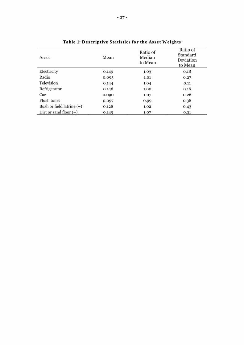
If we look at the relative importance of each of the eight characteristics in each

country, we find very little variation from one country to another. Table 1 reports the

cross-country means of the weights on the eight characteristics (scaled so that these

mean weights sum to unity8), along with the ratios of each median and standard

deviation to its respective mean. The table shows that the standard deviations are quite

small, and that the medians are close to the means, indicating an approximately

symmetrical distribution. We therefore construct a cross-country assets index for the

kth quintile of the nth country as follows:

astkn = Σh sh·zhkn

where h = 1,…,8 indexes the assets, sh is the weight on the hth asset, taken from the first

column of Table 1 (Σh sh = 1), and zhkn indicates the fraction of households in the quintile

possessing the asset. In the case of bush latrines and dirt floors, zhkn indicates the

fraction of houses without the characteristic. As can be seen from Table 1, there is not a

great deal of variation sh, so results from an alternative definition of wealth with h∀ sh

= 0.125 yields results very similar to the ones reported below.

8 The numbers in the table are subject to rounding error.

- 9 -

The assets index astkn is the first of our endogenous well-being indicators, yjkn.

Two other endogenous well-being indicators are selected from the HNP dataset.

Representing achievements in education, the first is the fraction of adults in quintile k

aged 15 to 49 who have completed grade five, denoted schkn. The second represents

achievement in health and is the child mortality rate, and is the annual number of

deaths in quintile k of children under five years of age per 1,000 live births. It is

denoted morkn. These indicators were chosen partly on the basis of data coverage, being

available for each quintile in each of our 48 countries.9 Well-being is treated as an

increasing function of each of the three endogenous variables. Achievements in each

have intrinsic worth as they are indicative of people exercising their reasoned agency.

They also have positive instrumental value with respect to each other and many

additional well-being outcomes.

To these variables we add the fertility rate in quintile k, denoted ferkn. Taken

from the HNP database, this variable is defined as the average number of live births per

women aged 15 to 49. We view this variable as an endogenous well-being outcome

indicator and thus one of the yjkn. On the one hand it could be argued that higher

fertility represents higher intrinsic achievement in health, and is indicative of people

exercising their reasoned agency with respect to well-being. On the other hand one can

argue that higher fertility inhibits achievement in well-being by placing greater stress

on household and other resources, and can lead to lower achievements in health,

education and other well being outcomes. Donors tend to view fertility in this light, as

evidenced by their support for family planning schemes in many developing countries.

Yet whether well-being is an increasing or decreasing function of fertility will depend

on the relative strengths of these properties. In absence of this information fertility 9 We also considered alternative definitions of wealth, education and health, using: (i) uniform

asset weights to define material well-being, (ii) the fraction of women reading a newspaper at

least once a week to measure education and (iii) the mortality rate for children under 12 months

to measure health. Using these measures produced very similar results to those reported below.

- 10 - enters our econometric model as an endogenous control variable. While interactions

between it and the other endogenous well-being variables play an important role in our

model we draw no inferences about its overall impact on well-being. 10

*** Table 1 about here ***

Table 2 provides data on the unconditional correlations of the well-being

indicators, again disaggregating by quintile. The signs on individual correlation

coefficients are unsurprising. Wealth and education are positively correlated. Wealth

and child mortality are negatively correlation or, put differently, wealth and health

positively correlated given that the latter is a decreasing function of child mortality. The

same applies to education and health. Wealth, education and health are each negatively

correlated with fertility. Note also that the correlations are generally highest for

quintiles 3 to 5 and lowest for quintiles 1 and 2 (the poorest). This suggests that the

variation in outcomes for richer households is more systematic, and may be more

closely correlated with observable independent characteristics; the variation among

poorer households may have a larger stochastic element. These characteristics indicate

that in our econometric analysis it would be unwise to try to impose any a priori

structure on the covariance matrix of residuals for each well-being indicator and each

quintile. Variances and covariances are unlikely to be uniform across quintiles, let alone

across indicators. Outcomes at the upper end of the assets distribution are likely to be

somewhat more predictable than those at the lower end.


Another characteristic of the well-being indicators is that three of them are not

normally distributed.11 In the case of astkn there are observations close to both the

10 A further comment on our selection of well-being variables is warranted. It should be

acknowledged that we will be looking at relationships between what might be considered as

stock variables (assets and schooling) and a flow variable (mortality), the difficulties of which

are well-known.

- 11 - upper and the lower theoretical bounds. At the former all of the households in the

quintile possess all of the assets in the wealth index, while at the latter or none do.

Likewise, in some quintiles, nearly all adults have completed schooling to grade five

and in others none have. The distribution of morkn is left-skewed. We therefore use the

following logistic transformations of these variables in our least-squares econometric

analysis:

lgastkn = ln(astmin-astkn) - ln(astmax-astkn)

lgschkn = lnschkn – ln(1-schkn)

lgmorkn = lnmorkn – ln(1-morkn)

where astmin and astmax are, respectively, the minimum and minimum theoretical values

of the assets index. We use a logarithmic transformation for the fertility rate, lnferkn.

4. Econometric Approach

Equations (1) and (2) will take the following specific form. All variables are for

the current period, unless otherwise indicated.

lgyjkn =F( αjk + Σi ≠ j βmij·yikn + Σ p φm

jp·xknp + θmjlnaidkn)+ ujkn (3a)

for j = (astkn, schkn, morkn) and

lnyjkn = αjk + Σi ≠ j βmij·yikn + Σpφm

jp·xknp + θmjlnaidkn + ujkn (3b)

for j = (ferkn). F(.) is the Normal cumulative density function. xknp is the value of the pth

exogenous conditioning variable for the nth country in which quintile k resides and ujkn

is a residual. The superscript m will be defined below. We identify and discuss these

variables below. Our aid equation is

lnaidkn = π + Σp ρp xknp + λqlnzknq + υkn (4)

where lnaidkn is the natural logarithm of aid disbursed relative to the population of the

nth country.

11 Further details about the distributions of all four variables are available on request from the

authors.

- 12 -

The exogenous conditioning variables in equations (3a) and (3b), xknp, capture

national characteristics that vary across countries but not across quintiles within a

country. We will include in our model variables to capture factors relating to

geography, history and culture. Given significance in previous related studies (for

example, Easterly and Levine, 1997), we will include a dummies for countries in Africa

(africa) and Hispanic America (hisp). The geographic variables also include a binary

dummy variable for whether or not the country in question has a maritime coastline

(coast), mean annual temperature in 0.1 degrees centigrade (temp),a logarithmic

measure of the capital value of natural resources in US Dollars (natres), surface area in

square kilometres (size) and the fraction of the population at risk from malarial

infection (mal). The history variables are binary dummies indicating whether or not the

country was colonised by Great Britain (british) or by France (french). The culture

variables are the fractions of the population that is Christian (chrsp), Roman Catholic

(rcap), Muslim (musp). Full definitions of these variables are provided in Table 3. Data

on them was obtained from CIA (1997), Dixon and Hamilton (1996), Hoare (2005),

Krain (1997), La Porta et al. (1998) and McArthur and Sachs (2001).12

Special consideration was given to the choice of aid instruments in equation (4),

znq. Our dataset limits the number of such variables that can be included in this

equation. We consider two alternative sets of conditioning variables. By using two

alternative sets of conditioning variables we can make judgements about the robustness

of the interpretations of our results to choosing one set over another. The first

instrument set contains three distance variables, each expressed as a natural logarithm.

These variables are the distance in kilometres from each country’s national capital to

Paris, Tokyo and Washington, respectively. They are denoted as paris, tokyo and wash.

The amount of aid a country receives is likely to be a decreasing function of the distance

12 A number of other exogenous conditioning variables were employed in preliminary

econometric testing, including the ethno-linguistic fractionalization index (Krain, 1997) and the

Sachs-Warner index of trade openness (Sachs and Warner, 1995).

- 13 - to these cities, which are the national capitals of some of the largest aid donor nations

in terms of the volume of aid provided globally. Data on the distance variables were

obtained from WorldAtlas (2009). The second instrument set contains one variable

only, which is the ratio of ODA disbursements to ODA commitments over the five years

prior to the first year of measurement of the aid variable, lnaidkn. An ODA commitment

is the amount of funds donors make available to recipients for disbursement. A failure

to disburse the full amount of aid made available by donors in any particular year is can

be attributed to a lack of capacity on the part of the recipient to allocate aid funds. It

can also be attributed to a lack of will on the part of the recipient to disburse aid funds

or even a lack of knowledge of the level of funds made available to it. Donors in these

circumstances can reduce the aid committed in the next year to the recipient in

question to such an extent that the amount disbursed would also decline. The amount

of aid disbursed in period t would on these grounds be expected to be an increasing

function of the ODA disbursement to commitment ratio in period t-1. All data required

to calculate this variable were taken from OECD (2009).

A priori restrictions on the φmjp coefficients will allow us to identify (most of)

the βmij coefficients that capture the interactions between the four well-being indicators.

These restrictions are summarised in Table 3. We allow the conditional cross-country

mean of each well-being indicator, αjk, to vary across quintiles, so we are in effect fitting

a fixed effects model. We have 4 5 48 observations of yjkn, and hence 960

observations of the residuals ujkn. We do not wish to assume any restriction on the

correlation of residuals across indicators or across quintiles, so the model is fitted by

stacking 21 regression equations – one for each j and each k, plus one for aid – and

estimating the coefficients in each equation simultaneously using the efficient three

stage least squares method. Note that all of the φmjp coefficients appear in the aid

equation, so the impact of the different development indicators on donor aid choices is

not identified. The aid equation is in reduced form, and modelling donor choices is an

exercise for a future paper.

- 14 -


With only 48 countries, we do not have enough degrees of freedom to allow each

of slope coefficients, βij, φjp and θi, to vary across quintiles. We do, however, have

enough data to allow these coefficients to vary for two groups of quintiles. We will

obtain coefficients for quintiles 1 and 2 and 3 to 5, thus in equations (3a) and (3b) m =

if k є {1, 2} or m = 2 if k є {3, 4, 5}. It follows that these coefficients should be

interpreted as representing the mean effects of the corresponding explanatory variables

across all countries and all quintiles. Quintiles 1 and 2 contain the poorest people

surveyed in each of the countries in our dataset, and almost all of them are will be

poor by any reasonable international standard. Identifying the impact of aid on these

people is the objective of this paper, and this guides our aggregation of quintiles. We

acknowledge, however, that in a number of countries in our sample, quintile 3 could

also contain people who are poor according to international standards.13

Our conclusions regarding aid effectiveness will be based primarily on the

impacts that apply in equilibrium, having solved out the four equations for the well-

being indicators. We have no firm a priori expectations regarding the relative impact of

aid on each population sub-group. One might expect that the primary beneficiaries of

aid are the poorest quintiles. Given, however, the complexity of aid effects, difficulties

in reaching the very poorest communities, incentives for donors to by -pass the poorest 13 In partial recognition of this issue, an earlier version of this paper reported results for the

impact of aid on groups quintiles not formed according to the country in they are located but

according to absolute poverty lines. Low, middle and high groups were formed according to each

well-being indicator. For child mortality, for example, the low group consisted of quintiles with

less than 100 deaths per 1000 live births, the middle group consisted of those with 100 to 200

deaths and the high group consisted of those with more than 200 deaths per 1000 live births.

Results obtained were very similar to those reported later in this paper, with aid having the

greatest beneficial impacts on the middle group for all well-being variables. The high poverty

group benefited more than the low poverty group only in terms of the impact on child mortality.

Further details are available on request from the authors.

- 15 - and the greater ability of richer groups to take advantage of the opportunities that aid

can general, it remains uncertain whether these groups will benefit most from aid. We

cannot rule out an impact on the poorest groups even if donors cannot and do not

attempt to reach them. There could well be indirect impacts, such as those on economic

growth, employment or business activity that might affect the poor in one way or

another. These impacts could also benefit the rich. Donors often support health and

education programmes in developing countries. Rich groups can access the services

provided by these programmes, and can therefore benefit from them. We leave it to the

data to help detect and disentangle these various aid impacts.

5. Results

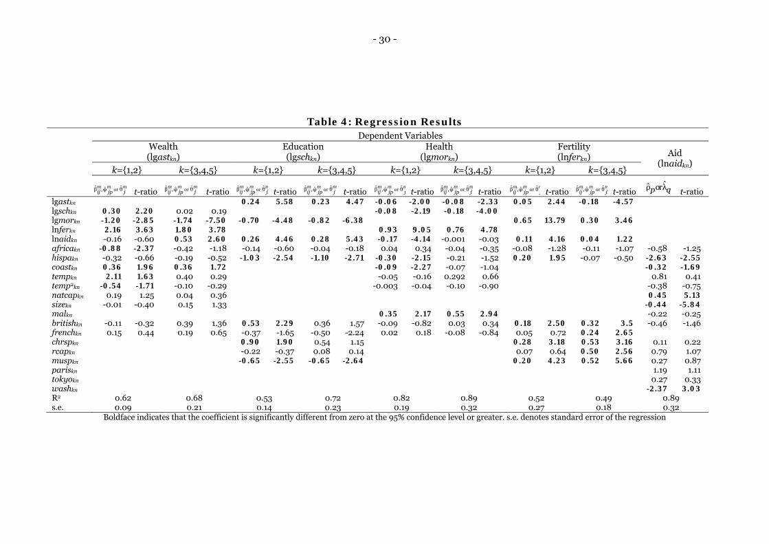
Regression results obtained from estimating equations (3a), (3b) and (4) for the

four well-being indicators are reported in Table 4. These results have been obtained

with the quintiles 1 to 2 and 3 to 5 groupings, and using the distance variable

instruments in the aid equation, equation (4). Results obtained an alternative grouping

(into quintiles 1 to 3 and 4 to 5), and results using the aid instrument discom, are

similar to those shown in Table 4, and yield the same overall conclusions. Our

conclusions would appear, therefore, to be robust with respect to the choice of quintile

groups and aid equation instrument. For this reason and also for the sake of brevity we

do not provide a detailed reporting of these results. We first discuss the results relating

to the interaction of the four well-being variables, and hence the estimates of βmij, which

as mentioned are estimates of the partial derivatives among these variables, and then

turn to the primary interest of this paper, which is the impact of aid on well-being

across the population sub-groups.


Most of the estimated βmij coefficients are significantly different from zero at the

95 percent level or higher. Greater wealth is associated higher schooling in quintiles 1

and 2, higher fertility in quintiles 1 and 2 and 3 to 5 and lower mortality in quintiles 1

and 2 and 3 to 5. Higher schooling is associated with higher wealth and lower mortality

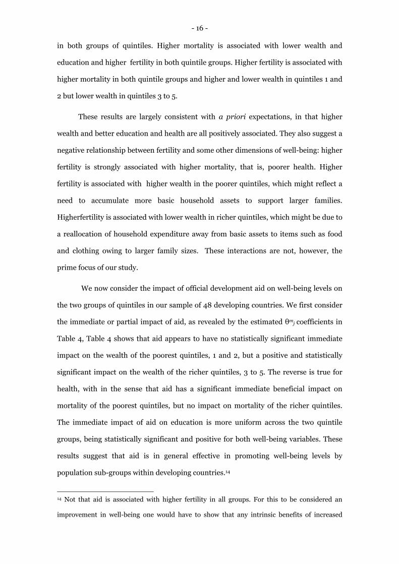
- 16 - in both groups of quintiles. Higher mortality is associated with lower wealth and

education and higher fertility in both quintile groups. Higher fertility is associated with

higher mortality in both quintile groups and higher and lower wealth in quintiles 1 and

2 but lower wealth in quintiles 3 to 5.

These results are largely consistent with a priori expectations, in that higher

wealth and better education and health are all positively associated. They also suggest a

negative relationship between fertility and some other dimensions of well-being: higher

fertility is strongly associated with higher mortality, that is, poorer health. Higher

fertility is associated with higher wealth in the poorer quintiles, which might reflect a

need to accumulate more basic household assets to support larger families.

Higherfertility is associated with lower wealth in richer quintiles, which might be due to

a reallocation of household expenditure away from basic assets to items such as food

and clothing owing to larger family sizes. These interactions are not, however, the

prime focus of our study.

We now consider the impact of official development aid on well-being levels on

the two groups of quintiles in our sample of 48 developing countries. We first consider

the immediate or partial impact of aid, as revealed by the estimated θmj coefficients in

Table 4, Table 4 shows that aid appears to have no statistically significant immediate

impact on the wealth of the poorest quintiles, 1 and 2, but a positive and statistically

significant impact on the wealth of the richer quintiles, 3 to 5. The reverse is true for

health, with in the sense that aid has a significant immediate beneficial impact on

mortality of the poorest quintiles, but no impact on mortality of the richer quintiles.

The immediate impact of aid on education is more uniform across the two quintile

groups, being statistically significant and positive for both well-being variables. These

results suggest that aid is in general effective in promoting well-being levels by

population sub-groups within developing countries.14

14 Not that aid is associated with higher fertility in all groups. For this to be considered an

improvement in well-being one would have to show that any intrinsic benefits of increased

- 17 -

More revealing are equilibrium or total impacts of aid, those which take into

account the simultaneous interactions between the endogenous variables in our system

of equations. Equilibrium impacts, obtained using the estimates of the βmij coefficients

reported in Table 4, are summarized in Table 5. The impacts are those which result

from exogenous shocks to each endogenous variable. Owing to the forms in which the

endogenous variables appear in our system of equations, shocks were imposed, one at a

time, on (astmin-astkn) - (astmax-astkn) schkn/(1-schkn), morkn/(1-morkn) and aidkn. The

impacts are measured as percentage changes in these variables. We introduce a shock

to the wealth equation that induces a ten percent increase in (astmin-astkn) - (astmax-

astkn) relative to its initial equilibrium level, and calculate the impacts on all of the well-

being variables in the subsequent equilibrium. We do the same for the education and

aid equations, imposing a ten percent increases in schkn/(1-schkn) and aidn. For the

health equation we model ten percent decreases in morkn/(1-morkn). The resulting

impacts are those that apply on average for each quintile group in each country. We

report bootstrapped t-ratios to judge whether these impacts are statistically significant.

Particular emphasis is given to overall gains from each shock, which are obtained by

summing the absolute values of statistically significant impacts. These statistics are the

“sum of impacts” statistics shown at the bottom of Table 5.


The impacts of exogenous ten percent changes provide some interesting insights

into the interactions between wealth, health and education. Increases in health are

associated with the largest overall improvements in the well-being variables in

equilibrium. We base these conclusions on the sum of impacts statistics in Table 5.

Improvements in health also result in the largest well-being gains for both the quintile

groups under consideration. For the richer quintiles, this outcome is due to the impact

of health on education, but also due to reductions and subsequent multiplier impacts

fertility outweigh its negative instrumental impacts. This is an interesting result given donor

programs aimed at lowering fertility in many developing countries.

- 18 - on health. For the poorer quintiles it is due to further improvements in health. That the

largest well-being gains are due to improvements in health would suggest that donors

should attempt to increase the impact of aid on mortality, alongside continuing totarget

increases in education. It should be acknowledged that from a well-being perspective

what matters is the weight attached to each outcome under consideration in a well-

being production function. In absence of such information, one is tempted to attach

equal weights to health, wealth and education. If this is accepted, our results suggest

that donors should target health. If we assume that what ultimately matters to donors is

the well-being levels of residents of countries to which they provide aid, then this would

provide additional justification for targeting health.

We now turn to the main interest of our paper - the impact of aid. As shown in

the last two columns of Table 5, aid has statistically significant equilibrium impacts on

all well-being variables. It results in significant improvements for both quintile groups

in all well-being variables, with the exception of the wealth of the poorer quintiles. For

all well-being variables, it is the richer quintiles that benefit most from aid. With

respect to education, for example, a ten percent increase in aid increases schooling by

among the richer quintiles by 7.28 percent, compared to 4.75 percent for the poorer

quintiles. For health, it results in declines in mortality of 3.51 percent and 2.61 percent,

respectively, for these groups.15

That the richer households in the 48 developing countries under consideration

benefit more from aid than their poorer counterparts is further emphasised by the sum

of impacts results shown in the bottom rows of Table 5. While both groups benefit on

average from aid, these results indicate that it is the richer group of quintiles that is the

principal beneficiary of aid in terms of its overall impact on levels of wealth, health and

education. These results will be both good and bad news for many with an interest in

official aid. The good news is that they provide evidence of aid working for the poor will

15 In equilibrium, exogenous increases in aid are also associated with statistically significant

declines in fertility, but only for quintiles 3 to 5.

- 19 - be good news to many observers of aid. The bad news is that they provide evidence of it

working least for this group.

The results in Table 5 are based on a model that fits the data well, but embodies

a functional form that does not necessarily provide the most intuitive results for policy-

makers. For this reason, we now translate the results for (astmin-astkn) - (astmax-astkn),

schkn/(1-schkn) and morkn/(1-morkn) into results for astkn, schkn and morkn. These results

are presented in Table 6. It shows the impact of a doubling of aid, from the actual levels

allocated these countries. A doubling of aid is chosen given the public pressure placed

on donors to increase aid by this margin in order to enhance progress towards the

Millennium Development Goals adopted by the United Nations (United

NationsMillennium Project, 2005), and a willingness of a number of donors achieve

such an increase. Individual quintile specific impacts are shown in Table 6, but bear in

mind that the differences between quintiles 1 and 2 and between quintiles 3 to 5 are a

consequence of the non-linear functional form of the model. 16 The largest impacts are

either on education or wealth. Among individual quintiles, it is the middle quintile,

quintile 3, that tends to do best from a doubling of aid. The predicted increase in the

number of adults within this quintile with schooling is 12.9 percentage points, while the

child mortality within it falls by 2.5 percentage points. In this sense aid seems to have

its greatest benefit for the average person within recipient countries. The poorest and

richest quintiles tend to do worst. The poorest, quintile 1, benefits least of a doubling of

16 The differences in the impacts of aid between quintiles shown in Table 6 are a function of

different mean values in a non-linear model, and are therefore slightly artificial. The quintiles

most affected by this will be those at either ends of the logistic function, quintiles 1 and 5. One

way to control for this is to apply the model parameters for quintiles 1 and 2 to the data for

quintile 5 and those for quintiles 3 to 5 to the data for quintile 1. Applying this method yields

larger impacts of the doubling of aid for quintile 1 and the reverse for quintile 5, but does not

alter the conclusion that the middle quintiles benefit most from this exogenous increase in aid.

- 20 - aid in terms of its impact on wealth. It benefits by roughly the same margins as the

richest quintiles, 4 and 5, with respect to the impact on education and health.


6. Conclusion

This paper models the impact of official foreign aid on the well-being levels of

population sub-groups in 48 developing countries. Well-being is defined in terms of

achievement with respect to wealth, health and education. Population sub-groups are

delineated on the basis of asset ownership, which was interpreted as a measure of

wealth. The special interest of the paper was on the impact of aid on the well-being of

the poorest sub-group, defined as the bottom two quintiles of households, in absolute

terms and relative to other sub-groups the countries under consideration.

It was found that aid is associated with improvements in most of the well-

being variables under examination. To this extent the findings of the paper are

consistent with the majority finding of the recent aid-growth literature, which is that

growth would on average be lower in the absence of aid. Aid seems to have the largest

beneficial impact on education. The paper also found, however, find that the poorest

quintiles benefit on average the least from aid. While many observers will be

heartened by evidence that the poorest groups might at least benefit from aid,

evidence of them benefitting least will be of significant concern. It should also be of

concern to donors since popular support for aid programs is premised on the

assumption or at least hope that these programs primarily benefit the poorest groups

in recipient countries.

That the poorer groups in developing countries benefit least from aid is a critical

finding and if supported by subsequent research findings has enormous implications

for aid delivery, especially in light of the expected scaling-up of world aid flows. One

obvious implication is that while aid might increase overall living standards in

developing countries, this could be at the cost of the living standards of the poor falling

further behind those of the rich in these countries. Whether such an outcome is

- 21 - observed will depend on other drivers of living standards gaps between these groups,

but the results of this paper would suggest that aid might make these gaps larger than

would be the case such external assistance. If donor governments are concerned about

this outcome then they clearly need to strive harder to ensure that the interventions

they fund, now and in the future, better serve the poorest people in recipient countries.

One means of achieving this is for donors to more effectively target health, given the

findings of this paper. Alternatively, donor governments could allocate more funds to

agencies that can be shown to better reach the poorest people in developing countries.

- 22 -

Appendix

*** Table A1 about here***

- 23 -

References

Alkire, S. (2002), ”Dimensions of Human Development”, World Development, Vol. 30,

No. 2, pp. 181–2005.

Anand, S. (2004), “The Concern for Equity in Health”, in S. Anand, F. Peter and A. Sen

(eds), Public Health, Ethics and Equity, Oxford: Oxford University Press.

Arndt, C., S. Jones and F. Tarp (2010), “Aid, Growth, and Development: Have We

Come Full Circle?”, Journal of Globalisation and Development, Vol. 1, Iss. 2, pp.

1-27.

Burnside, C. and D. Dollar (2000), “Aid, Policies and Growth”, American Economic

Review, Vol. 90, No. 4, pp. 847-868.

CIA (1997), World Factbook, Washington DC.

Deaton, A. (2009), Instruments of Development: Randomization in the Tropics, and

the Search for the Elusive keys to Economic Development, NBER Working Paper

No. 14690, National Bureau of Economic Research, Washington, DC.

Dixon, J. and K. Hamilton (1996), “Expanding the Measure of Wealth”, Finance and

Development. December, pp. 15-18.

Duflo, E., R. Glennerster and M. Kremer (2008), “Using Randomization in

Development Economics Research: A Toolkit”, in T.P Schultz and J. Strauss

(editors), Handbook of Development Economics, Vol. 4, Amsterdam: Elsevier.

Clemens, M., S. Radelet and R. Bhavnani (2004), Counting Chickens when they Hatch:

The Short-term Effect of Aid on Growth, Centre for Global Development Working

Paper No. 44, Washington DC: Centre for Global Development.

Easterly, W. (2003), “Can Foreign Aid Buy Growth?”, Journal of Economic

Perspectives, Vol. 17, No. 3, pp. 23-48.

Fielding, D. and S. Torres (2009), “Health, Wealth, Fertility, Education, and

Inequality”, Review of Development Economics, Vol. 13, No. 1, pp. 39-55.

- 24 - Feyzioglu, T., V. Swaroop and M. Zhu (1998), “A Panel Data Analysis of the Fungibility

of Foreign Aid”, World Bank Economic Review, Vol. 12, No. 1, pp. 29-58.

Franco-Rodriguez, S., M. McGillivray and O. Morrissey (1998), “Aid and the Public

Sector in Pakistan: Evidence with Endogenous Aid”, World Development 26

(1998): 1241-1250.

Gang, I. and H. Khan (1991), “Foreign Aid, Taxes and Public Investment”, Journal of

Development Economics, Vol. 24), pp. 355-69.

Gomanee, K., O. Morrissey, P. Mosley and A. Verschoor (2005a) “Aid, Government

Expenditure, and Aggregate Welfare”, World Development, Vol. 33, No. 3, pp.

355-370.

Gomanee, K., S. Girma and O. Morrissey (2005b), “Aid, Public Spending and Human

Welfare: Evidence from Quantile Regressions”, Journal of International

Development, Vol. 17, No. 3, pp. 299-309.

Hansen, H. And F. Tarp (2001), “Aid and Growth Regressions”, Journal of Development

Economics, Vol. 64, No. 2, pp. 547-570.

Heller, P. (1975), “A Model of Public Fiscal Behaviour in Developing Countries: Aid,

Investment and Taxation”, American Economic Review, Vol. 65, pp. 429-45.

Kanbur, R. (2001), "Economic Policy, Distribution and Poverty: The Nature of

Disagreements", World Development, Vol. 29, No. 6, pp. 1083-1094.

Kosack, S. (2003) “Effective Aid: How Democracy Allows for Development Aid to

Improve the Quality of Life”, World Development, Vol. 31, pp. 1-22.

McGillivray, M., S. Feeny, N. Hermes and R. Lensink (2006), “Controversies over the

Impact of Development Aid: It Works, It Doesn’t, It Can, but that Depends …”,

Journal of International Development, Vol. 18, No. 7, pp. 1031-1050.

Mosley, P., J. Hudson and A. Verschoor (2004), “Aid, Poverty Reduction and the New

Conditionality”, Economic Journal, Vol. 114, pp. F217-F243.

- 25 - Organisation for Economic Co-operation and Development (OECD) (2009),

International Development Statistics On-line,

http://www.oecd.org/dataoecd/50/17/5037721.htm

Organisation for Economic Co-operation and Development (OECD) (2011),

Development Aid Reaches an Historic High in 2010, Paris: OECD.

Pack, H and J.R. Pack (1990), “Is Foreign Aid Fungible? The Case of Indonesia”,

Economic Journal, Vol. 100, pp. 188-94.

Pack, H. J.R. Pack (1993), "Foreign Aid and the Question of Fungibility", Review of

Economics and Statistics, Vol.75, pp. 258-265.

Rajan, R.G. and A. Subramanian (2008), “Aid and Growth: What Does the Cross-

Country Evidence Really Show?”, Review of Economics and Statistics, Vol. 90,

No. 4, pp. 643-665.

Roodman, D (2007), "The Anarchy of Numbers: Aid, Development, and Cross-Country

Empirics," World Bank Economic Review, Vol. 21, No. 2, pp. 255-277.

Sachs, J. D. and A.M. Warner, (1995) “Economic Reform and the Process of Global

Integration”, Brookings Papers on Economic Activity, pp. 1-118.

Sen, A. (1999), Development as Freedom, New York: Random House.

United Nations Millennium Project (2005), Investing in Development: A Practical

Plan for Achieving the Millennium Development Goals, New York: United

Nations Development Program.

WorldAtlas (2009), WorldAtlas.Com, http://www.worldatlas.com/

World Bank (2003), World Development Report 2004: Making Services Work for

Poor People, Oxford University Press, New York.

World Bank (2004), Health, Nutrition and Poverty Data,

http://devdata.worldbank.org/hnpstats/pvd.asp

- 26 - World Bank (2009), World Development Indicators 2009, World Bank, Washington

DC.

United Nations Development Program (UNDP) (1990), Human Development Report

1990, New York: Oxford University Pres.

- 27 -

Table 1: Descriptive Statistics for the Asset Weights

Asset Mean Ratio of Median

to Mean

Ratio of Standard Deviation to Mean

Electricity 0.149 1.03 0.18

Radio 0.095 1.01 0.27

Television 0.144 1.04 0.11

Refrigerator 0.146 1.00 0.16

Car 0.090 1.07 0.26

Flush toilet 0.097 0.99 0.38

Bush or field latrine (–) 0.128 1.02 0.43

Dirt or sand floor (–) 0.149 1.07 0.31

- 28 -

Table 2: Unconditional Correlations between Well-being Variables

Wealth (astkn)

Education (schkn)

Health (morkn)

Quintile 1 schkn 0.48 morkn -0.51 -0.55 ferkn -0.36 -0.25 0.43 Quintile 2 schkn 0.65 morkn -0.67 -0.67 ferkn -0.55 -0.48 0.67 Quintile 3 schkn 0.72 morkn -0.74 -0.74 ferkn -0.69 -0.66 0.81 Quintile 4 schkn 0.75 morkn -0.79 -0.79 ferkn -0.75 -0.76 0.87 Quintile 5 schkn 0.71 morkn -0.83 -0.83 ferkn -0.65 -0.73 0.86

- 29 -

Table 3: Variable Definitions and Model Structure Endogenous Variables Definition lgastkn logistic transformation of the assets index for quintile k of country n lgschkn logistic transformation of the fraction of adults aged 15 to 49 that has completed primary education in quintile k of country n lgmorkn child mortality rate in quintile k of country n lnferkn natural logarithm of the average number of live births per woman aged 15 to 49 in quintile k of country n lnaidkn natural logarithm of net official development assistance disbursed to the country n, as a ratio of its population, in which quintile

k resides Exogenous Variables Definition Appearing in Equation for africakn dummy variable taking the value of one if for quintile k if n is an African

country or zero if otherwise lgastkn lgschkn lnferkn lgmorkn lnaidkn

hispakn dummy variable taking the value of one if for quintile k if n is a Hispanic country or zero if otherwise

lgastkn lgschkn lnferkn lgmorkn lnaidkn

coastkn dummy variable taking the value of one if the country n in which quintile k resides has a coastline

lgastkn lgmorkn lnaidkn

tempkn temperature in Celsius of the country n in which quintile k resides lgastkn lgmorkn lnaidkn temp2kn temperature-squared in Celsius of the country n in which quintile k

resides lgastkn lgmorkn lnaidkn

natreskn natural resource capital value of the country n in which quintile k resides lgastkn lnaidkn sizekn size of country n in which quintile k resides lgastkn lnaidkn malkn fraction of the population at risk from malaria in country n in which

quintile k resides lnaidkn

britishkn dummy variable taking the value of one if for quintile k if n is a former British colony country or zero if otherwise


frenchkn dummy variable taking the value of one if for quintile k if n is a former French colony or zero if otherwise


chrspkn fraction of the population that is Christian in country n in which quintile k resides

lgschkn lnferkn lnaidkn

rcapkn fraction of the population that is Roman Catholic in country n in which quintile k resides


muspkn fraction of the population that is Muslim in country n in which quintile k resides


discomkn ratio of per capita ODA disbursements to ODA commitments to the country n in which k resides, over the five years prior to the first year of measurement of our aid variable

lnaidkn

pariskn distance in kilometres to Paris from national capital of the country n in which quintile k resides

lnaidkn

tokyokn distance in kilometres to Paris from national capital of the country n in which quintile k resides

lnaidkn

washkn distance in kilometres to Washington from national capital of the country n in which quintile k resides

lnaidkn

- 30 -

Table 4: Regression Results Dependent Variables Wealth

(lgastkn) Education (lgschkn)

Health (lgmorkn)

Fertility (lnferkn) Aid

(lnaidkn) k={1,2} k={3,4,5} k={1,2} k={3,4,5} k={1,2} k={3,4,5} k={1,2} k={3,4,5}

m m mij jp jorˆ ˆˆβ ,φ θ

t-ratio


t-ratio

m m mij jp jorˆ ˆˆβ ,φ θ t-ratio


t-ratio




m m mij jp jorˆ ˆˆβ ,φ θ t-ratio p q

ˆρ̂ orλ t-ratio

lgastkn 0.24 5.58 0.23 4.47 -0.06 -2.00 -0.08 -2.33 0.05 2.44 -0.18 -4.57 lgschkn 0.30 2.20 0.02 0.19 -0.08 -2.19 -0.18 -4.00 lgmorkn -1.20 -2.85 -1.74 -7.50 -0.70 -4.48 -0.82 -6.38 0.65 13.79 0.30 3.46 lnferkn 2.16 3.63 1.80 3.78 0.93 9.05 0.76 4.78 lnaidkn -0.16 -0.60 0.53 2.60 0.26 4.46 0.28 5.43 -0.17 -4.14 -0.001 -0.03 0.11 4.16 0.04 1.22 africakn -0.88 -2.37 -0.42 -1.18 -0.14 -0.60 -0.04 -0.18 0.04 0.34 -0.04 -0.35 -0.08 -1.28 -0.11 -1.07 -0.58 -1.25 hispakn -0.32 -0.66 -0.19 -0.52 -1.03 -2.54 -1.10 -2.71 -0.30 -2.15 -0.21 -1.52 0.20 1.95 -0.07 -0.50 -2.63 -2.55 coastkn 0.36 1.96 0.36 1.72 -0.09 -2.27 -0.07 -1.04 -0.32 -1.69 tempkn 2.11 1.63 0.40 0.29 -0.05 -0.16 0.292 0.66 0.81 0.41 temp2kn -0.54 -1.71 -0.10 -0.29 -0.003 -0.04 -0.10 -0.90 -0.38 -0.75 natcapkn 0.19 1.25 0.04 0.36 0.45 5.13 sizekn -0.01 -0.40 0.15 1.33 -0.44 -5.84 malkn 0.35 2.17 0.55 2.94 -0.22 -0.25 britishkn -0.11 -0.32 0.39 1.36 0.53 2.29 0.36 1.57 -0.09 -0.82 0.03 0.34 0.18 2.50 0.32 3.5 -0.46 -1.46 frenchkn 0.15 0.44 0.19 0.65 -0.37 -1.65 -0.50 -2.24 0.02 0.18 -0.08 -0.84 0.05 0.72 0.24 2.65 chrspkn 0.90 1.90 0.54 1.15 0.28 3.18 0.53 3.16 0.11 0.22 rcapkn -0.22 -0.37 0.08 0.14 0.07 0.64 0.50 2.56 0.79 1.07 muspkn -0.65 -2.55 -0.65 -2.64 0.20 4.23 0.52 5.66 0.27 0.87 pariskn 1.19 1.11 tokyokn 0.27 0.33 washkn -2.37 3.03 R2 0.62 0.68 0.53 0.72 0.82 0.89 0.52 0.49 0.89 s.e. 0.09 0.21 0.14 0.23 0.19 0.32 0.27 0.18 0.32

Boldface indicates that the coefficient is significantly different from zero at the 95% confidence level or greater. s.e. denotes standard error of the regression

- 31 -

Table 5: Equilibrium Impacts of Shocks in Endogenous Variables 10 Percentage Changes in Wealth Education Health Aid Estimate t-ratio Estimate t-ratio Estimate t-ratio Estimate t-ratio

Impacts on

Wealth k=1,2 11.67 2.56 3.53 0.50 0.42 0.02 1.87 0.35

k=3,4,5 11.67 2.37 4.42 1.06 22.78 1.32 7.63 2.16

Education k=1,2 3.46 1.06 12.02 2.68 19.26 1.50 4.75 2.74

k=3,4,5 6.63 2.17 14.35 4.57 25.58 2.11 7.28 3.21

Health

k=1,2 -0.96 -0.48 -2.36 -0.85 -27.42 -2.56 -2.61 -2.02

k=3,4,5 -4.82 -1.94 -4.63 -2.23 -24.78 -2.78 -3.51 -1.65

Fertility

k=1,2 -0.02 -0.01 -1.34 -0.88 -17.68 -1.67 -0.53 -0.65

k=3,4,5 -3.55 -1.97 -2.19 -1.47 -11.57 -1.96 -2.07 -1.77

Sum of Impacts

k=1, 2 11.67 12.02 27.42 7.36

k=3, 4, 5 26.67 18.98 50.36 18.42

k=1, ..., 5 38.34 31.00 77.78 25.78 The respective wealth, health and aid variables are (astmin-astkn) - (astmax-astkn), schkn/(1-schkn), morkn/(1-morkn) and aidkn. Boldface indicates that the estimated impact is significantly different from zero at the 95% confidence level or greater. All impacts represented as percentage changes. Sum of Impacts statistics are obtained by summing the absolute values of significant changes.

- 32 -

Table 6: Equilibrium Impacts of Doubling Aid

Quintile (k)

Wealth (astkn)

Education (schkn)

Health (morkn)

Before After Change Before After Change Before After Change

1 13.3 14.9 1.6 30.8 38.6 7.8 14.6 12.4 -2.2

2 21.2 23.5 2.3 40.9 49.4 8.5 13.8 11.7 -2.1

3 30.4 43.2 12.8 49.8 62.7 12.9 12.8 10.3 -2.5

4 43.1 56.9 13.8 61.1 72.7 11.6 10.9 8.7 -2.2

5 66.9 77.9 11.0 78.5 86.1 7.6 7.8 6.2 -1.6

All changes are in percentage points.

- 33 -

Table A1: Countries Included in the Analysis

Country Survey Year Country Survey Year

Bangladesh 2000 Madagascar 1997

Benin 2001 Malawi 2000

Bolivia 1998 Mali 2001

Brazil 1996 Mauritania 2001

Burkina Faso 1999 Morocco 1992

Cambodia 2000 Mozambique 1997

Cameroon 1998 Namibia 2000

Central Afr. Rep. 1995 Nepal 2001

Chad 1997 Nicaragua 2001

Colombia 2000 Niger 1998

Comoros 1996 Nigeria 1990

Cote d'Ivoire 1994 Pakistan 1990

Dominican Rep. 1996 Paraguay 1990

Egypt 2000 Peru 2000

Ethiopia 2000 Philippines 1998

Gabon 2000 Rwanda 2000

Ghana 1998 South Africa 1998

Guatemala 1999 Tanzania 1999

Guinea 1999 Togo 1998

Haiti 2000 Uganda 2001

India 1999 Vietnam 2000

Indonesia 1997 Yemen 1997

Jordan 1997 Zambia 2002

Kenya 1998 Zimbabwe 1999

does aid work for the poor?

Documents