1111111111111111111111111111111111111111111111111111111111111111

3 1176 00166 4649

DOE/NASA/0029-1 NASA CR-1 65380

----------~

Wind Flow Characteristics in the W8kisol------Large Wind Turbines

Volume I-Analytical Model Development

W. R. Eberle Lockheed Missiles and Space Company, Inc.

September 1981

Prepared for National Aeronautics and Space Administration Lewis Research Center Under Contract DEN 3-29

for U.S. DEPARTMENT OF ENERGY Conservation and Renewable Energy Division of Wind Energy Systems

LIBRARY COpy NOV 4 1981

U,NGL~Y RESE.t\RCH CENTER L:L3RP,RY, NASA

H • .;~.:?TON, VIRGINIA

111111111111111111111111111111111111111111111 NF01568

- -- --------

https://ntrs.nasa.gov/search.jsp?R=19810025059 2018-05-28T09:57:33+00:00Z

NOTICE

This report was prepared to document work sponsored by

the United States Government. Neither the United States

nor its agent, the United States Department of Energy,

nor any Federal employees, nor any of their contractors,

subcontractors or their employees, makes any warranty,

express or implied, or assumes any legal liability or

responsibility for the accuracy, completeness, or useful­

ness of any information, apparatus, product or process

disclosed, or represents that its use would not infringe

privately owned rights.

DOE/NASA/0029-1 NASA CR-165380

Wind Flow Characteristics in the Wakes of Large Wind Turbines

Volume I-Analytical Model Development

W. R. Eberle Lockheed Missiles and Space Company, Inc. Huntsville, Alabama

September 1981

Prepared for National Aeronautics and Space Administration Lewis Research Center Cleveland, Ohio 44135 Under Contract DEN 3-29

for U.S. DEPARTMENT OF ENERGY Conservation and Renewable Energy Division of Wind Energy Systems Washington, D.C. 20585 Under Interagency Agreement EX-76-1-01-1 028

/lJ t:j/ - 33(9CJ2':i:f ---------------------------------------------------------------~/

FOREWORD

The material in this report documents the efforts of the first phase of an overall program conducted by Lockheed Missiles and Space Company, Inc., of Huntsville, Alabama, under NASA contract DEN3-29. The firs.t phase of the program called for a computer model of the wind turbine wake, while the second phase dealt with wake measurements on the Mod-OA wind turbine at Clay­ton, New Mexico.

The computer program of this report is considered an initial calculation procedure for the wake development of wind turbines because additional expansions and refinements are possible to make the program more comprehensive. Areas for further consider­ation include additional methods for calculating the effects of atmospheric turbulence, non-equal vertical and lateral wake growth rates, and power recovery factor based on real turbine power char­acteristics.

iii

1.0 SUMMARY .....

2.0 INTRODUCTION ..

TABLE OF CONTENTS

3.0 DESCRIPTION OF WAKE MODEL.

3.1 Approach

Turbulence relationships.

Wake geometry . . .

3.2 Data Input ......... .

Page 1

3

5

5

5

6

8

3.3 Calculation of Program Constants. 11

Recalculation of input geometric parameters 11

Calculation of the initial wake radius. .. 12

Calculation of wake growth due to ambient turbulence . . . . . . . . . . . 12

Calculation of wake characteristics at the end of Region 1. . . . 17

Downwind extent and radius at end of Region II. . . . . . . . . . 21

3.4 Wake calculations in Region III. 22

Wake growth in Region III . . . . . 22 Turbine power factor. . . . . 25

3.5 Wake plots·. . . . . . . . . . . . 29

3.6 Calculation of Wind Speed Profiles

Coordinates

Region I ..

Region I II. . .

Region II .

3.7 Calculation with Ground Effect. 3.8 Calculation of Wind Speed.

v

29

29

31 31

32 32

33

4.0 COMPARISON WITH PREVIOUS MODEL ..

4.1 Wake Growth Rate Due to Ambient Turbulence . . . . .

4.2 Support Tower ........ . 4.3 Calculations for Region I . 4.4 Wake Growth in Region III .

5.0 SAMPLE PLOTS. 5.1 Wake Plots.

Abramovich solutions Wakes in ground effect .

5.2 Effect of Principal Wake Parameters Effect of ambient turbulence . . Effect of initial velocity ratio Effect of turbine rotor hub height . Effect of the power law exponent .

6.0 CONCLUSIONS ..

7.0 REFERENCES.

APPENDICES A - LIST OF SYMBOLS . . . . . . . . . . . . . B - PROGRAM LISTING . . . . . . . . . . . . . C - WAKE CALCULATIONS ON THE TI-59 CALCULATOR D - ALTERNATIVE ALGORITHMS FOR CALCULATION OF

. . 51

51

52 52

· 53

· 55 55

· 55 · 57

• . 58

• 58

59

· 60 · 60

. .143

. . . 144

.145

.152

· 177

THE DOWNWIND EXTENT OF REGION I ....... 196

vi

1

1.0 SUMMARY

One of the proposed approaches to reducing the consumption of fossil fuels (in particular, petroleum and natural gas) in the United States is the use of large wind turbines. It is expected that such turbines will be constructed in arrays in large fields of wind turbines. To minimize cost, it is desired to space the turbines as close to each other as possible. However, the turbines must not be spaced so closely that a turbine lies within the wake of another turbine and thereby the output power of the downwind turbine is reduced.

In order to determine the appropriate spacing between turbines, a research program was initiated to characterize the recovery of the wake behind a large wind turbine. The research program had two aspects. The first was the develop­ment of an anlytical model of wake recovery downwind of the turbine. The analytical model was developed to calculate the wake properties as functions of the downwind coordinate and to generate wind speed profiles (i.e., wind speed as a function of the lateral coordinate for selected altitudes and wind speed as a function of the vertical coordinate) at selected distances downwind of the turbine. The inputs to the model included wind speed, ambient turbulence, and turbine geometric parameters. The second aspect of the program was an experimental program to measure the wake behind the Mod-OA wind turbine at Clayton, New Mexico. The Lockheed laser Doppler velocimeter was used to make the measurements. This volume contains a description of the analytical model development.

The analytical model development is based upon the results presented by G. N. Abramovich in "The Theory of Turbulent Jets". The term "jet" is used to describe a flow surrounded by another flow of a different velocity, regardless if the velocity of the inner flow is less than or greater than that of the surrounding flow. Although the Abramovich results were taken as the basis for the analytical model for turbine wakes, several modifications of the Abramovich results were necessary. The Abramovich model assumes that the initial jet emanates from an opening. Therefore, it was necessary to add calculations to relate the turbine to the initial wake as presented by Abramovich. Second, the results of Abramovich were developed for flow with no ambient turbulence. Therefore, the effects of ambient turbulence were added to the Abramovich model for the turbine wake model.

2

The wake growth rate due to ambient turbulence was taken from atmospheric diffusion theory as developed by F. Pasquill. The method of combining the wake growth rate from the Abramovich model with the wake growth rate due to ambient turbulence was taken from the work of P. B. S. Lissaman from a prior model for the wake recovery behind large wind turbines.

Third, the concept of a turbine power factor, which is the ratio of the power generated by a turbine centered in the wake of another turbine to that generated by a turbine in the free stream air, was added to the model.

The mathematics of the wake model was written in a FORTRAN computer program. The FORTRAN computer program was implemented on a PDP-IO computer using the DISPLA graphics package for graphical presentation of results. In addition to the computer program, a version of the wake program was formulated for the TI-59 program­mable calculator. The calculator version of the wake program is presented in an appendix.

Several runs of the computer program were made to illustrate the effect of wake variables on wake recovery. The effect of ambient turbulence, initial wind speed deficit in ,the wake, the height of the turbine rotor hub above the ground, and the power law coefficient for the free stream wind were investigated. The results of these effects are presented in figures in the report.

The principal indicator of wake recovery is the turbine power factor. Much of turbine operation occurs under conditions of neutral atmospheric stability, represented by Pasquill stability class D. For this condition and for an initial velocity ratio of 1.5 (typical for large wind turbines), the turbine power factor is approximately 0.5, 0.75, 0.9, and 0.96 at 10, 20, 35, and 50 rotor radii downwind, respectively.

3

2.0 INTRODUCTION

One of the proposed approaches to reducing the consumption of fossil fuels (in particular, petroleum and natural gas) in the United States is the use of large wind turbines. It is expected that such turbines will be constructed in arrays in large fields of wind turbines. To minimize cost, it is desired to space the turbines as close to each other as possible. However, the turbines must not be spaced so closely that a turbine lies within the wake of another turbine and thereby the output power of the downwind turbine is reduced.

In order to determine the wake characteristics of tur­bines, a research program was initiated to characterize the recovery of the wake behind a large wind turbine. The research program had two aspects. The first was the development of an analytical model of wake recovery downwind of the turbine. The second aspect of the program was an experimental effort to measure the wake behind the Mod-OA wind turbine at Clayton, New Mexico. The Lockheed laser Doppler velocimeter. (LDV) was used to make the measurements. This report presents the re­sults of the first phase of the investigation, which involved the development of an analytical wake model to calculate the wind speed profile (i.e., wind speed as a function of the lateral coordinate for selected altitudes) at selected dis­tances downwind of the turbine. The principal inputs to the model include wind speed, ambient turbulence, and turbine ge­ometry and operating parameters.

The initial wake behind a wind turbine can be represented as a volume of flow of lower momentum than the surrounding flow. This mass gradually acquires the speed of the surrounding flow as it progresses downwind. Some features are similar to those of a wake behind a bluff body as described in reference 1, while other features are like those of coflowing jets as de­scribed in reference 2. There are few published reports on the detailed wake behind wind turbines. Templin (ref. 3) and Crafoord (ref. 4) have made theoretical estimates of large scale effects, that is, without considering detailed flow near each turbine. Some experimental wind tunnel work has been done by Ljungstrom (ref. 5), while more detailed wind tunnel work has been conducted by Builtjes (ref. 6). A comprehensive re­view of this work is given by Lissaman (ref. 7).

The analytical model presented in this report was de­veloped through an evolutionary process. At the beginning of the contract covering the work reported herein, a subcontract was issued to AeroVironment, Inc. (Lissaman and Walker) for

4

the development of an analytical model and computer program for the wake flow. The model developed by AeroVironment was based on previous work done for the Swedish National Board for Energy Source Development. The report describing the details of the AeroVironment model and calculation procedure is refer­ence 8. The general principles of the model are also described in reference 9, which has a wider distribution than reference 8.

Upon close examination of the AeroVironment model, it was determined that there were certain aspects of the model which could be modified to improve the accuracy of the modeling of the fluid mechanics of the wake. There were also some re­finements in the model which were originally requested, but which, in retrospect, should have little influence on the overall results. The effects of these refinements were deemed to be less than the uncertainties of some of the major assumptions of the model. The revised version of the model is contained in this report.

Both versions of the analytical model are based on the theory of co flowing jets as presented by Abramovich in ref­erence 2. The term "jet" is used to describe a flow emanating from an opening into a larger surrounding coflowing flow. The velocity of the jet may be greater or less than that of the surrounding flow. In the application of the co flowing jet to the analysis of wind turbine wakes, ambient turbulence must be considered. Thus, for both the AeroVironment model and the revised model as reported herein, the main task was the addition of the effect of ambient turbulence and the ground plane to the Abramovich model, computerizing the results, and providing automated graphical output for the wake character­istics.

This report contains a description of the analytical model and a comparison with the earlier AeroVironment version. Sample calculations using the analytical model are presented, and the effects of the principal input parameters on wake characteristics of a large wind turbine are explored. Also included in the report are appendixes containing a listing of the computer model, a version of the model for use on the TI-59 programmable calculator, and a discussion of the alter­nate algorithms considered in the development of the model.

5

3.0 DESCRIPTION OF WAKE MODEL

3.1 Approach

The mathematical model used for calculating the wind speed profiles in the wakes of large wind turbines is ~escribed in this section. The basic concept of the mathematical model is that the wind speed profile, in the wake is of different math­ematical form in different regions of the wake (as defined later), but this form is uniquely defined in each region at each position downwind of the turbine. For each profile region, knowing the wake radius at the beginning of the region and the wake growth rate in the region, the wake radius can be determined at any desired downwind location. Then, for a given mathematical form of the wind speed profile, the centerline wind speed is uniquely determined by the condition that the momentum deficit is conserved from the initial wake to the downwind location.

Turbulence relationships,. - The total effective growth rate of the wake is glven by the Pythagorean sum of the growth rate due to the mechanical turbulence (i.e., turbulence generated because of velocity gradients in the flow) and that due to the ambient turbulence. The growth rate due to mechanical turbulence is obtained by the experimental results of Abramovich (Ref. 2), and the growth rate due to ambient turbulence is assumed constant along the wake for a given value of the atmospheric turbulence. The Pythagorean sum (i.e., square root of the sum of the squares) was chosen because the total kinetic energy of the combined turbulence equals the sum of the kinetic energy of the mechanical turbulence and the kinetic energy of the ambient turbulence.

Abramovich (ref. 2) has done extensive work on coflowing jets in fluids. Much of his work has been based on experimental results with no ambient turbulence in the jet or in the surrounding fluid. There are two mechanisms of momentum transfer in the coflowing jets for which Abramovich has presented results. The first mechanism is the result of the viscosity of the air acting on the velocity gradients in the flow. This mechanism of momentum transfer could be represented by the Navier-Stokes equations for laminar flow (although Abramovich does not use the Navier-Stokes equations). The second mechanism of momentum transfer is turbulence generated by velocity gradients in the flow. Because of energy extraction by the turbine rotor, the wind speed of the air flowing through the rotor is reduced, thus creating a stream tube of flow with a wind speed less than that of the surrounding free stream. The velocity gradient across the flow creates turbulence. This creates an eddy viscosity (ref. 10), which increases the momentum transfer in the flow. This mechanism of momentum transfer is much more significant than momentum transfer in laminar flow.

6

In the following discussion, the parameters calculated from Abramovich are termed as being due to "mechanical turbulence" because it is the gradients in the flow which cause the turbulence which causes the momentum transfer in the cases which Abramovich has studi~d. This term is used to distinguish the effects which Abramovich has presented in ref. 2 from the effects of ambient turbulence which were not included in the effects which Abramovich included in his analysis.

The wake growth rate due to ambient turbulence has been taken from the theory of diffusion of pollutants by turbulence in the atmosphere. Because of recent regulations related to air quality, the theory of pollutant dispersion has been developed extensively over the past few years. The relationship between the dispersion of pollutants and the transfer of momentum in a wake is given by Abramovich.

Wake Geometry. - The wake of a single turbine is shown in Figure 3-I,as idealized for the unbounded flow (i.e., no effect of the ground). The wake is divided into three regions for the calculations. The wake radius in the first two regions increases linearly with downstream distance at a rate set by the effective turbulence, which is a combination of the mechanical turbulence and the ambient turbulence. The influence of the mechanical turbulence diminishes and asymptotically approaches zero as the wake moves downwind. Eventually, the effect of the mechanical turbulence becomes negligible, and the wake growth is essentially determined by ambient turbulence alone .. In order to accurately model wake growth with a diminishing influence of mechanical turbulence, the wake boundary of Region III was calculated by a numerical integration. The details of the geometry and flow in these regions will be discussed in the following sections.

In the initial region (Region I), the potential core is that portion of the wake which has been unaffected by the shear between the wake and the outer (ambient) flow. Region I extends to X = X , the point at which the shear due to the outer flow has comp¥etely eroded the potential core of uniform flow down­stream of the extraction disk. Wind speed profiles across the wake.in this region are not self-similar at various downstream locations due to the change in relative size of the core flow and the turbulent mixing zone. At the end of Region I, a continuous shear layer-like wind speed profile has completely developed but is represented by a slightly different functional form from that used later in the far wake regime. The transition region, Region II, allows for the smooth transition of the

7

completely developed wind speed profile of Region I to that used in the far wake, which is self-similar for all subsequent downstream locations.

Region I also includes the expansion of the wake from the diameter of the physical extraction disk, Rd , to the expanded slipstream value, RO' that is, the slipstream expansion due to potential effects. The computer model assumes that this expansion occurs at the station of the disk itself so that the wake develops from R = RO at X = O. Reasons for this assumption are discussed in a following section.

The wake growth rate is identical for Regions I and II, and is given by a combination of ambient and mechanical turbulence as discussed in the following sections. The end of Region II occurs at XN = nXH, where n is derived from the form of t~e wind speed profile in Region I and the form of the wind speed profile in Region III as described by Abramovich. The wake radius is calculated at the end of Region I and at the beginning of Region III based upon a momentum balance with the initial wake and the form of the wind speed profiles at each of the respective locations. The downwind extent of Region II is then calculated from the ratio of these radii and the wake growth rate in Region I.

Region III is the far wake. In the initial part of Region III, wake growth is controlled by a combination of mechanical and ambient turbulence. Further downwind, the effect of mechanical turbulence asymptotically approaches zero, and the wake growth is essentially controlled by ambient turbulence alone. In the numerical integration in Region III, wake growth due to mechanical turbulence is never mathematically e limin,a ted. However, its influence asymptotically approaches zero.

Figure 3-1 also shows the notation to be used for the geometrical parameters in the following discussion. Upper case R denotes the wake radius in physical units. Notation for lower case r is similar to that shown in Figure 3-1, but denotes wake radius normalized by the turbine rotor radius, Rn. The normalized radius of the potential core is r J • The normalized outer radius of the wake at the end of Region R is r Zk . The notation, r 2 , is used for the normalized outer radius at any general location in the wake. The normalized downwind distance at which Regions I and II end are xH and xN ' respectively. In the following discussion, upper case U tlenotes wind speed in physical units. Lower case u denotes wind speed which has been normalized by the free stream wind speed, Uoo •

8

The following sections describe the computer model. The description follows the calculation procedure of the computer program sequentially, giving derivations of equations used as appropriate. The equations follow the development of Abramovich (ref. 2) closely, and no derivation of equations taken directly from Abramovich is given here. The reader is referreA to ref. 2 for derivations of these equations. A flow diagram for the computer program is shown in Figure 3-2. A list of symbols is given in Appendix A, and a program listing is given in Appendix B. The equation number in the following description is underlined when the equation is used directly in the computer program. In the program listing in Appendix B, the equation numbers for equations presented in this section are given.

In addition to the computer program, a version of the wake model was developed for the TI-59 programmable calculator. The TI-59 version of the model is presented in Appendix C. The TI-59 version of the program uses the same equations as those developed in this section for the computer model.

3 .2 Data Input

The first step of the program is data input. Table 3-1 shows the input data and card formats for the input data. The definitions of input parameters are given in Table 3-2.

The output of the program consists of a set of plots. The plots consist of the wake radius, the wind speed deficit at the center of the wake, the wind speed at the center of the wake, and the turbine power factor (ratio of the power which would be generated by an identical turbine in the wake of the first turbine to that power which would be generated if the downwind turbine were in the free stream wind) plotted as functions of the downwind coordinate. At the user's option, the geometric parameters may be plotted in physical units or as normalized by the rotor radius. Plots of the wind speed in the wake as a function of the lateral coordinate for eight altitudes for each of the selected downwind locations are also made. At the option of the user, the plots are normalized by the free stream wind speed at the hub altitude or by the free stream wind speed at the altitude at which the plots are made. In addition, a plot showing the vertical wind speed profile at each of the downwind locations of the lateral wind speed profiles is made.

The parameter, as' is an indication of the atmospheric turbulence. It may be entered in one of two ways. First, it may be entered as the standard deviation of wind direction as measured by tower-mounted anemometers. Alternatively, the atmospheric turbulence may be represented by the Pasquill

9

atmospheric stability class. The stability class varies from class A (highly unstable atmosphere) to class F (highly stable atmosphere). Table 3-3 (taken from ref. 11) provides a key to stability classes.

"Strong" incoming solar radiation corresponds to a solar altitude of greater than 60° with clear skies; "slight" inso­lation corresponds to a solar altitude from 15° to 35° with clear skies. Cloudiness will decrease incoming solar radiation and should be considered along with solar altitude in deter­mining solar radiation. Incoming radiation that would be strong with clear skies can be expected to be reduced to moderate with broken (5/8 to 7/8 cloud cover) middle clouds and to slight with broken low clouds. These methods will give representative indications of stability over open country or rural areas, but are less reliable for urban areas. This difference is due primarily to the influence of the city's larger surface roughness and heat island effects upon the stability regime over urban areas.

In general, inter turbine spaceing for wind turbines should be based on Pasqui11 stability class D, which corresponds to neutral atmospheric stability. From Table 3-3, stability classes other than class C and class D occur only when wind speeds are too low for turbine operation near rated power. Since wake recovery will be faster for class C and for class D (because of greater ambient turbulence for class C), class D is the appropriate design condition.

The value of the initial ve10ctiy ratio, m, to be used as input may be determined from one-dimensional momentum theory in the following manner taken from Ref. 12. Let U be the free stream wind speed, UT be the wind speed through the turbine disk, and Uo be the initial wind speed of the wake (i.e., after expansion due to potential effects as discussed in the following discussion). For the one-dimensional momentum analysis, power is extracted from the disk uniformly over the disk area, A. The axial thrust on the disk is

T = Momentum flux in - Momentum flux out

or

T (3-1) .

where m is the mass flow rate of air passing through the turbine disk, and p is the mass density of the air. Also, from pressure considerations, the thrust can be expressed as

10

+ -T = A(p -p ) (3-2)

where p+ and p are the static pressures on the upwind and down­wind sides of the turbine, respectively. Applying the momentum equation (Bernoulli's equation) on the upwind side of the turbine gives

+ P +~pU 2 = P +~pU 2

00 2 00 2 T

where Poo is atmospheric static pressure. of the turbine

(3 - 3)

On the downwind side

(3-4)

+ -Subtracting these equations to get (p -p ) and using equation (3-2) gives

(3 - 5)

Equating this with equation (3-1) gives

(3-6)

From equation (3-6), it is seen that the wind speed through the turbine is the average of the free stream wind speed ahead of the turbine and the wind speed in the expanded wake of the turbine.

The axial induction factor, a, is defined by

(3-7)

Therefore, from equation (3-6),

(3-8)

and the initial velocity ratio, m, is

U 1 00

m - = (3 - 9) Uo 1-2a

11

The initial velocity ratio can also be expressed in terms of the turbine output power. Because power is given by the mass flow rate times the change in kinetic energy, ~KE, of the wind flowing through the turbine, the power, Poo ' is

(3 -10)

or, substituting for UT from equation (3-7) and for Uo from equation (3-8) and simplifying,

Poo

= 2pAUoo3 a(l-a)2 (3-11)

The power, P , has a maximum at a = 1/3 and a minimum at a = 1. Therefore, i~ the turbine is operating at its maximum power for the given free stream wind speed, m = 3. If the turbine is not extracting the maximum power available at its free stream wind speed, the appropriate value of "a" T.1Ust be calculated from equation (3-11). An iterative solution is necessary because equation (3-11) is a cubic equation in "a". The power to be used in equation (3-11) is the power extracted from the wind, not the electric power output of the generator. The aero­dynamic power is the power extracted from the air by the tur­bine blades. For an operating tubine, it may be obtained from the output power and the generator and shafting efficiencies.

After the values of the input parameters have been read, the program writes the values of the input parameters.

3.3 Calculation of Program Constants

Geometric constants for the program are calculated first. The constants include the wake growth rate due to ambient turbulence, the initial wake radius, the downwind extent of Region I, the wake radius at the end of Region I, the downwind extent of Region II, and the wake radius at the end of Region II.

Recalculation of in ut eometric arameters. - The program allows input 0 geometrlc parameters ln p YSlca1 units or in rotor radii. If they have been input in physical units, they are corrected to units of rotor radii.

h = H /Rd a a (3-12)

12

Zo = ZO/Rd

6z = 6Z/Rd

6y = 6Y/Rd

(3-13)

(3-15)

Calculation of the initial wake radius. - From the momentum analysis presented above, the wake expands from the wind speed through the physical extraction disk, UT, to the initial wake wind speed, UO' Let Rd be the radius of the turbine disk, and let RO be the radlus of the wake after expansion to speed, UO' The mass flow rate of air through the disk is

From equations (3-6) and (3-9)

R 2 o R 2

d

= =

(3-16)

m+1 = (3-17)

2

Therefore, the initial wake radius is given in terms of the disk radius as

(3-18)

For the calculation of wake parameters, as indicated previously, the results of Abramovich were derived for mechanically-generated turbulence only (no ambient turbulence). In the following sections, the results of Abramovich are modified to include the effects of ambient turbulence.

Calculation of wake growth due to ambient turbulence. -The program next calculates wake growth due to ambient turbu­lence. The theory for the turbulent dispersion of plumes (e.g., pollutants) in the atmosphere is used as the basis for the calculation of wake growth due to ambient turbulence. There are three steps in the following discussion. The first step is the determination of the plume growth as measured by

13

the concentration of atmospheric pollutants. The second step relates the concentration of atmospheric pollutants to the wind speed deficit in the wake of turbines. The third step relates the profile parameters for profiles used for pollution concen­tration work to the profile parameters for profiles used for wakes.

In atmospheric dispersion work, the Gaussian distribution is used to describe the concentration of pollutants. This distribution is given in axisymmetric form as

=

~X c

where X = concentration of pollutants

(3-19)

Xc = concentration of pollutants at plume center Xoo = free stream concentration of pollutants (usually zero) r = radial coordinate a = pollution dispersion coefficient.

As mentioned previously, the atmospheric turbulence may be input as the Pasquill stability class or as the standard devia­tion of wind direction. Input as the Pasquill stability class is considered first. Figure 3-2 of Ref. 11 gives a a5 a function of x, the distance downwind of the pollution source,for the six Pasquill stability classes. That figure is reproduced here and shown as Figure 3-3. From this figure, the following values for da/dx were calculated.

DERIVATIVE OF POLLUTION DISPERSION COEFFICIENT FOR PASQUILL STABILITY CLASSES

Pasquill stability class

A

B C D

E F

da/dx 0.212

0.156

0.104

0.069

0.050

0.034

14

Reference 13 relates the Pasquill stability class to ae' the standard deviation of, wind direction of the atmosphere. This relation is given as follows.

STANDARD DEVIATION OF WIND DIRECTION FOR PASQUILL STABILITY CLASSES

Pasquill stability class

A

B

C

D

E

F

ae (degrees)

25.0

20.0

15.0

10.0

5.0

2.5

A least squares curve fit of the data given in the two pre­ceding tables gives

, da (3-20)

dx

Since a = 0 at x = 0,

a(x) = 0.031xe· 08ae (3-21)

If the atmospheric turbulence is input as a Pasquill stability class, table pg. 13 is used to generate a value for da/dx. If the atmospheric turbulence is input as a value of as' equation (3-20) is used to generate a value for da/dx.

As the second step, it is desired to relate the distribution of concentration of pollution to the distribution of wind speed' deficits. In the discussion preceeding equation (5.25), Abramovich states that according to Prandtl's old and new assumptions of free turbulence, the dimensionless profiles of temperature and wind speed are the same, but according to

15

Taylor's theory of free turbulence, they differ. In the discussion preceeding equation (5.27), Abramovich states that the mechanism of lateral transfer of heat and of admixture is the same; consequently, the profiles of concentration difference must be similar to the profiles of temperature difference. This is stated in equation (5.27) of Abramovich. Combining this result with equation (5.25) of Abramovich gives

= J~u = ~ Lm ~u--=u-c c co

where U = wind speed in the wake U = wind speed at the center of the wake U~ = free stream wind speed.

(3-22)

Combining equation (3-22), the result of the Taylor theory mentioned above, with equation (3-19) for a Gaussian wind speed profile

(3-23)

As a third step, it is desired to relate the a of the Gaussian wind speed profile given by equation (3-23) to the wake radius, r 2 , for the wind speed profile used in the model presented hereln. In the far wake, the wind speed profile is given by equation (5.23) of Abramovich as

6u _ [ (r J. 5] 2 - - 1--6uc r Z

(3-24)

The wind speed profiles of equation (3-23) and (3-24) are very similar and are compared in Figure 3-4. In determining the relationship between a and r 2 , 6u is the same for both profiles, and the mass deficit is theCsame for both profiles. The equality of mass deficits is '

f -2ro/2a 2 2n6uc e r (3-25)

o

16

Dividing by 2TI~uc and integrating between the stated limits gives

or

= 2 70

r 2 Z

r Z = 1.97cr

(3-26)

(3-Z7)

Therefore, the wake growth rate due to ambient turbulence is

a = (dr 2/dx)a = 1.97(dcr/dx) (3-Z8)

where (dcr/dx) is obtained from the table on p. 13 or from equation (3-20) "according to the method of input of atmospheric turbulence.

The above derivation is based on the Taylor theory of free turbulence. This is the approach used by Abramovich, and Abramovich presents a curve (Figure 5.10 in Abramovich) which shows excellent agreement between experimental data and the Taylot theory. Therefore, the Taylor theory was accepted for use in this model. The Prandtl assumption is stated as

~x flu = (3-29)

which is analogous to equation (3-22) for the Taylor theory. Under the Prandtl assumption, equation (3-Z3) would be

(3-30) ~uc

Tracing through the derivation above gives the result

r 2 = 2.79cr (3-31)

Therefore, the Prandtl assumption can be used in the model by replacing the 1.97 in equation (3-28) with 2.79.

17

Calculation of wake characteristics at the end of Region I. -Let Uoo be the free stream wind speed, U be the initial wind speed in the wake Cc.f. equation (3-9))pand U be the local wind speed in the wake. Abramovich assumes the wind speed profile in Region I to be

Uo-U f (n) (1_n 1 • 5 }2 = = (3-32)

U -u o 00

where, in the notation of Figure 3-1,

n = = (3-33)

Equation (3-32) is based on experimental data.

By definition, the end of Region I is that point at which the potential core vanishes. Thus, the wind speed at the center of the wake at the end of Region I is U. A momentum balance between the initial wake and the gnd of Region I gives

R21 RO =----=

RO Rd 10.214+0.144m (3-34)

where R21/RO is given by equation (5.19) of Abramovich, and rO is given by equation (3-18).

From the equation for boundary layer growth given by his equation (5.1), Abramovich gives the length of the initial region of the wake as (equation (5.20))

(XH)m RO r O(l+m) =

RO Rd 0.27(m-l)/0.214+0.144m

The m subscript denotes that the quantity is associated with mechanically-generated turbulence (and is given by the Abram­ovich model).

18

Equation (3-34), which gives the wake radius when the potential core has been completely eroded, is derived from conservation of the momentum deficit from the initial wake, the fact that U = Uo at the center of the wake at the end of Region I, and the assumption of the wind speed profile given by equation (3-32). - It is therefore valid regardless of the presence or absence of ambient turbulence. Therefore, the presence or absence of ambient turbulence only affects the distance, XH, at which the end of Region I occurs.

In the development of the model, seven approaches for t~~ downwind extent of Region I were considered. The approaches are described and compared in Appendix D. Two of the approaches are slightly different in concept, but yield identical results. They are physically more justifiable than the other approaches and give numerical results that lie near the middle of the numerical results of all of the other approaches. Therefore, these two approaches have been selected for the model. The reader is referred to Appendix D for a description of the other five approaches.

Figure 3-S(a) shows Region I for the Abramovich solution. The three areas shown are the free stream flow, the potential core, and the boundary layer between the free stream flow and the potential core. Also shown is the line which passes through the initial wake boundary and the midpoint of the wake radius at the end of Region I. The effect of ambient turbulence is shown in figure 3-S(b).

The first approach is based upon the growth of the boundary layer, b. Under this approach, the downwind extent of Region I is defined as that point at which the width of the boundary layer is r2l. Since the wake radius ia also r2l at the end of Region I and

(3-36)

the radius of the potential core, rl' must be zero at this point. For mechanical turbulence, the growth rate of the boundary layer is

(3-37)

Furthermore, for this formulation, the ambient turbulence exists in both the free stream flow and in the potential core. Since

19

the ambient turbulence affects both sides of the boundary layer, and a is the wake growth rate due to ambient turbulence on one side of the boundary layer (since it was developed as the rate of growth of the wake radius), the total growth rate of the boundary layer is

db = (3-38)

dx

where the Pythagorean sum of the mechanical turbulence and the ambient turbulence has been used. Since the wake radius is r

Z1 at the end of Region I, the downwind extent of Region I is

r Z1

db/dx = (3-39)

An alternate approach to the downwind extent of Region I results from the assumption that the boundary layer develops about its own center. For this assumption, the erosion of the inner core, or the growth of the outer radius, is measured relative to the line passing from the initial wake radius to half the wake radius at the end of Region I, as shown in fig­ure 3-S(b). For the erosion of the inner core, let bl be the distance from the edge of the potential core to the midpoint of the boundary layer. Hence, for mechanical turbulence,

(db I ) = dx m

Adding the ambient turbulence from the inner core by the square root of the sum of the squares gives

Since b i = O.Sr Zl at the end of Region I,

(3-40)

(3-41)

20

(3-42)

[(0. 5T 21 )2 +a. 2 ] !z

(xH)m

It is noted that mUltiplying both the numerator and the denominator of equation (3-42) by 2 gives equation (3-39).

The same result is obtained when the growth of the outer radius of the wake is considered. Let b 2 be the distance from the mid point of the boundary layer to the outer radius of the wake. Then at the end of Region I

(3-43)

Adding ambient turbulence gives

db 2 [c~:~~lr +a'] !z

= dx

(3-44)

Since b 2 = 0.5r 21 at the end of Region I ,

0.5r 21 xH = [C. srZl)' +a' ] !z

(xH)m

(3-45)

which is identical to equation (3-42).

The parameter for the wind speed deficit at the center of the wake is

= u -u

00 c

u -u 00 0

(3-46)

21

which is the wind speed dificit at the centcr of the wake divided by the initial wind speed deficit. The c subscript denotes the wind speed in the center of the wake. Because the wind speed in Uo in the core of the initial region, ~uc = 1 in Region I.

Downwind extent and radius at end of Re ion II. - Region II is a transltion reglcn rom t e Wln spee pro lIe form of the initial wake to the wind speed profile form of the far wake. The form of the wind speed profile in Region I is given by equation (3-32). Using this form for the wind speed profile and the condition that the wind speed at the center of the wake is UO' the wake radius at the end of Region I (denoted by r 21 ) is glven by equation (3-34) and is derived from the fact tfiat the momentum deficit at the end of Region I must equal the momentum deficit of the initial wake. As shown later in the discussion of Region III, in Region III, the wind speed profile is of the form given by equation (3-53). Using the same conditions (i.e., wind speed at the center of the wake is Uo and the momentum deficit of the wake must equal the initial momentum deficit of the wake), the wake radius calculated is greater than r Z1 ' Let this wake radius be the wake radius at the end of Reglon II and be denoted by r 22 . The downwind extent of Region II is the distance required to allow wake growth from r 21 to r 22 at the wake growth rate of Region I. The downwind extent of Region II is given by

(3 - 4 7)

where n is taken from equation (5.124) in Abramovich as

IO.214+0.l44m 1-lo.134+0.124m n = (3-48)

l-lo.214+0.144m IO.134+0.124m

The wake growth rate in Region II is identical with that in Region I. Therefore, the wake radius at the end of Region II is given by (cf., Figure 3-1)

(3-49)

22

or, dividing by Rd gives

TZ2 = (3- SQ)

The relationship of equation (3-48) is derived solely from. the mathematical forms of the wind speed profiles in Region I and Region III and the assumption that the wake growth rate in Region II equals that in Region I. If these same assumptions are made in the presence of ambient turbulence (i.e., the presence of ambient turbulence does not change the form of the wind speed profile in Region I or in Region III, and the wake growth rate in Region II equals that in Region I), then the relation­ship of equation (3-48) is valid in the presence of ambient turbulence.

3.4 Wake Calculations in Region III

Wake growth in Region III. - Region III of the wake is the region in which the mechanically-generated turbulence decays. Thus, at the beginning of the region, wake growth is governed by both mechanically-generated turbulence and ambient turbulence. The wake growth due to mechanically-generated turbulence asymp­totically approaches zero as the downwind coordinate, x, increases. In Region III, the wind speed profiles are self­similar, that is, they have the same mathematical form at all downwind locations. If the applicable expressions from Abramovich are used, the wake growth must be calculated by numerical integration.

Let it be assumed that the wake radius, r , is known at distance, x, downwind of the turbine, where f2 and x are values of the wake radius and downwind distance which have been normalized by the rotor ra,dius, Rd. Let r 2 ' = r'}+l:lr . be a wake radius which is slightly larger than r 2 . It is desired to find the downwind distance at which the wake radius is r 2 '.

For the main region of the jet, the unnumbered equation preceeding equation (5.97) of Abramovich gives the wake radius as a function of the wind speed deficit at the center of the wake as

2u Iu

[

n -mn ] ~ (3-51)

23

where ~u is defined by equation (3-46) and c

n - n = 1 lu - 2u (3-52)

in the case of uniform fields of velocity and density at the initial cross section of the jet (equation following equation (5.39) of Abramovich).

In the main region of the jet, Abramovich assumes (based on experimental data) that the form of the wind speed profile in the far wake is

~u

tiD c

= u -u

CX> (3-53)

u -u CX> c

where U is the wind speed at the center of the wake. From this as~umed form of the wind speed profile, equation (5.86) of Abramovich gives

Al = 0.258 (3-54)

and

A2 = 0.134 (3-55)

Therefore, equation (3-51) is

(3-56)

Equation (3-56) is a momentum equation which equates the momentum deficit in the main region of the wake to the initial momentum deficit of the wake. Rearranging equation (3-56) to solve for ~uc gives

O.134~U2_(O.258m)~u + ____ T_O_2 __ c c 2 ( ) m-I r 2 m-I

= 0 (3-57)

or

= 3. 73{O. 258m _ fl(O. 258m)2 _ O. ~36ro 2 ] ~} m-I L m-I r 2 (m-l)

Z4

where the negative sign for the quadratic equation was chosen so that ~uc goes to zero as r Z becomes large.

From his equation (5.Z8), Abramovich assumes that the wake growth rate is directly proportional to the difference between the wind speed of the free stream flow and the wind speed at the wake center and is inversely proportional to the mean wind speed of the wake. Using the first part of equation (5.31) of Abramovich gives

dx ±c-­

dr Z

ZU 00

= 1+---U -U c 00

ZU 00', = 1------- (3-59)

~uc(Uoo-UO)

where the definition of ~u given by equation (3-46) has been used in the last term of the equation. Dividing by Uoo ' using the definition of m given by equation (3-9) and rearranging gives the wake growth rate due to mechanical turbulence (using c = -0.Z7 for m > 1) as

(drz) dx m

= O. Z7[ Zm (m-1)~u c

-1 J -1

(3-60)

The calculation procedure for wake growth in Region III is as follows. Let it be assumed that the wake radius, r Z' is known at distance, x, downwind of the turbine. Let r Z' = rZ+~r be a wake radius which is slightly larger than r Z. Let (dr7./dx) be the wake growth rate due to mechanically-generated turouletlte calculated from equation (3-60) for wake radius, r Z. The value of ~u used in equation (3-60) is calculated from equati?n (3-58)7 Let (dr7 /dx) , be ~he wake gr?wth rate due to mechanlcally-generated tUTbul~ce for wake radlus, r Z'. As before, the wake growth rate due to ambient turbulence is taken as a. Therefore, the total wake growth in the interval ~r between r Z and r Z' is given by

C: 2) e = {(Cdr 2/dX

)m: Cdr 2/ dX)m ')' +a 'J" (3-61)

The downwind distance, x', at which the wake radius is r Z' is given by

x' = x+----- (3-6Z) (drZ/dx)e

25

Equations (3-60) through (3-62) are solved iteratively, and r~ is thereby generated as a function of x. In the calculation procedure, the calculations of equations (3-58) and (3-60) are performed in Subroutine R3 since the calculations must be repeated many times for different values of r 2 and r 2 '.

If one of the downwind locations at which wind speed profiles are to be calculated is encountered during the numerical inte­gration of Region III, the wake radius at that point is retained. The wake radius at the desired value of x is obtained by linear interpolation between the values of x which bracket the desired value of x. The numerical integration is continued downwind until x > 50 or r 2 > 7, whichever occurs first.

Turbine power factor. - As mentioned previously, Subroutine R3 is used to perform the calculations of equations (3-58) and (3-60). The subroutine also calculates the turbine power factor which is defined as

P = PIP 00

where P = power which is generated by a turbine which is geometrically identical to another turbine and centered in the wake of the other turbine

Poo = power generated by the turbine in the free stream wind.

(3-63)

The geometry related to a wind turbine in the wake of another wind turbine is shown in Figure 3-6. This geometry represents a worst case condition because the downwind turbine is centered in the wake of the ~pwind turbine. For actual turbines, the wake oscillates because of changes in the wind direction. However, in the present analysis, it is asssumed that the downwind turbine is fixed in the center of the wake of the upwind turbine.

Immediately upwind of the turbine, the stream tube of the flow passing through the turbine expands from a radius, R , and wind speed U , to the disk radius, Rd , and the wind speed~ UT, through the turbine disk. It is assumed that the distance, ~x over which the potential effects occur (cf. equations (3-1) p, through (3-6)) is small compared with the distance between the turbines. Let A be the cross-sectional area of the stream tube in the freeOOstream. Let the turbine power for a turbine in the free stream air be

P = KA U 3 00 00 00

(3-64)

26

where, from comparison with equation (3-11), the constant, K, is

K = 2pAa(1-a)2/A co

(3-65)

For a turbine in the wake of another turbine, equation (3-64) must be modified to show the variation of the "free stream" wind speed across the stream tube for the downwind turbine. For a turbine in the wake of another turbine, the power is

R

p = 2 'IT Kj [uer)] 3R dR

o

or, normalizing R by Rd and normalizing U by Uco

P = 2UKUm3Rd2j[:'(r)]3r dr o

gives

Combining the definition of the turbine power factor from equation (3-63) with equations (3-64) and (3-66) gives

p p =

or

=

r

2 'IT KUco 3Rd 2 jEu er)] 3r dr o

(3-66)

(3-67)

(3-68)

(3-69)

From the conservation of mass in the stream tube upwind of the turbine, the mass flow rate of air thtough the turbine is

(3-70)

Using equation (3-6) for Ur and rearranging gives

R 2 = 00

27

U +UO 00 R 2

2U d 00

Dividing by R 2U and using the definition of m given in equation (3-9~ gives

(3-71)

(3-72)

The preceeding discussion has been related to the downwind turbine (i.e., the turbine which lies within the wake of the upwind turbine). The wake of the upwind turbine forms the free stream wind flow for the downwind turbine. In the far wake (Region III), the form of the wind speed profile is given by equation (3-53). Combining this equation with the definition of ~u given in equation (3-46) and the definition of m given in eqfiation (3-9) and dividing by Uoo gives

(3-73)

If the center of the downwind turbine coincides with the center of the wake with the wind speed profile given by equation (3-73), the turbine power factor is

For convenience in the derivation, let

(3-75)

Then

p = r:2 [11-3B [1-(:)'· sr.3B2 [1-GJ'· T-B' [I-G) .S] } dr (3-76)

28

(r )3 (r )".5 + [- 3B+18B 2 -15B 3] r

2

+ [·12B 2+20B 3] r

2

( r)6 Ir)' . 5 (r 9

+[3B2

-15B'] rZ

+6B\rz

-B';;) Ir dr

(3-77)

Integrating between the indicated limits and simplifying gives

_ Il-3B+3B2-B3 P = 2 +

. 2

The p~wer factor ~ can then be expressed explicitly ~s a f~nct1~n of.m and r2 by evaluating B from equation. (3-58) 1n conJunct1on w1th equation (3-18) and r from equation (3-72). The expression for B is' 00

B = 3. 731 {o . 2S8 - [0 . 06656 - 0 ~ :: 8 « 2) r } Figure 3-7 shows calculated values of P as a function of r 2 for three values of m as obtained from equation (3-78) and the above \ expression for B. This plot is not generated during the computer run.

This analysis was developed for a wake out of ground effect. That is, there is no effect of the ground plane and no wind shear because of the ground. Two other assumptions are involved. The first is that no significant wake growth occurs over the distance of the expansion of the stream tube from radius Roo to the disk radius Rn for the downwind turbine. The second assump­tion is that the ~xial induction factor, a, is the same for both turbines. Because the turbine power factor is based upon the form of the wind speed profile that exists in Region III, the turbine power factor is undefined in Regions I and II.

29

3.5 Wake Plots

As mentioned previously, the numerical integration in Region III is terminated when x > 50 or r 2 > 7, whichever occurs first. Four plots are then made. The first plot shows the wake radius, the wake width, and the height of the top of the wake above the ground as a function of the downwind coordinate, x. The wake width is

w = 2r 2

The height of the top of the wake above. the ground is

(3-79)

(3-80)

The second plot shows 6u as a function of x. The third plot shows the normalized win~ speed at the center of the wake, uc' This is obtained from rearranging equation (3-46) to give

(3-81)

and then dividing by Uoo to give

The fourth plot shows the turbine power factor as a function of the downwind coordinate, x, in Region III.

3.6 Calculation of Wind Speed Profiles

After the plots described above have been completed, plots of wind speed profiles are made. The first set of wind speed profiles shows the wind speed as a function of the lateral coordinate for eight altitudes specified by the input values of Zo and ~z. Plots are made for each of the input desired downwind locations. A plot of the vertical wind speed profile at the wake centerline is then made. A single plot shows the vertical wind speed profile at all of the downwind locations at which lateral wind speed profiles were made.

Coordinates. - If the downwind locations at which wind speed profiles are desired have been input in physical units, they are converted to units of rotor radii by

30

(3-83)

where the notation x~o denotes the downwind coordinate of the jth location at whicnJwind speed profiles are desired .

. During the calculation of the wake radius as previously described, the wake radius corresponding to each xdo is calculated and retained. Let r . be the wake radiu~ at x = xdo, For the xdj which are less thans*N J

(3-84)

For the xdo which are larger than xN' the values of r ° are retained aJ the values of the xdo are determined durlrtg the numerical integration of Region fII. The wake radius at xdj is obtained by linear interpolation between the values of x which were calculated in the numerical integration and which bracket xdj .

The generation of the lateral wind speed profiles begins at Z = Zo and y = 0 (axis of turbine). Values of the wind speed in the wake are calculated at increments, ~y, beginning at y = o. Once the value of y is in the free stream (indicated by u = 1), the free stream value of the wind speed is extended across the plot to y = 6 rotor radii. The altitude is then incremented by ~z, and the wind speed profile at the next alti­tude is generated. The process is repeated until wind speed profiles have been generated for eight altitudes. Since the lateral profiles are symmetrical about y = 0, the wind speed for only positive values of yare determined.

After the lateral wind speed profiles have been generated for a given downwind location, xdo, the vertical wind speed profile is generated. The vertic~l wind speed profile is cal­culated at y = 0 only. The profile begins at z = 0 with in­crements of the input value of ~y used for successive calcula­tions (i.e., ~z = ~y for this calculation).

The altitude of the point on the wake profile (y,z) rela­tive to the axis of the turbine, denoted by zv' is also calcu­lated. It is

Zv = z-ha (3-85)

where z is the altitude as measured from the ground.

31

Subroutine CALCU is used to calculate the wind speed in the wake for given values of y and z. The subroutine first calculates the radius of the point (y,z ) as v

r = (3-86)

Region I. - If xd" ~ xH' xd · is in Region I. The radius of the potential core is J

Consider n as defined by equation (3-33) where rZ = rsj. If n > 1, r is inside the potential core and

u = 11m

If n < 0, r is outside the wake boundary, and

u = 1 (3-89)

If 0 < n < 1, r is in the boundary layer. Rearranging equation (3- 32), dIviding by U , and us ing the de fini tion of m from equation (3-9) gives 00

u =

After the value of u is calculated, control is returned to the main program.

Region III. - If xdj > xN' xdj is in Region III. If r > r Z'

u = 1

If r < r Z' Subroutine R3 is called to calculate 8UC from equation (3-58). Then, with (U~-U) from equation (3-53) and (U~-Uc) from equation (3-46),

U -u 00

(3-92)

32

Dividing by Uoo and using the definition of m in equation (3-9) gives

(3-93)

For this equation it is seen that if r = r Z' u = 1. If r = o ,

u = HUc(l-~) (3-94)

which agrees with the definition of ~uc given in equation (3-46).

Region II. - If xH < xd' < xN' xn' is in the transition region. The wInd speed is 1Irtear1y inL~rpo1ated between the profile at the end of Region I and the profile at the beginning of Region III. The actual radius of the wake in Region II is used. Let uT be the value of u calculated from equations (3-33) and (3-90) USing the value of r/r Z in Region II. Let u III be the value of u calculated from equation (3-93) using the same value of r/r Z' At the beginning of Region III, ~uc = 1. Then, for Region II,

After calculation of u, control is returned to the main program.

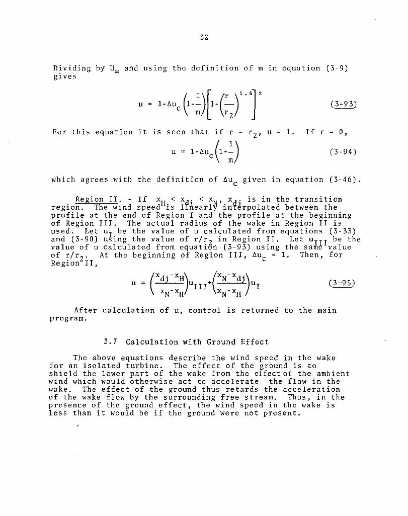
3.7 Calculation with Ground Effect

The above equations describe the wind speed in the wake for an isolated turbine. The effect of the ground is to shield the lower part of the wake from the effect of the ambient wind which would otherwise act to accelerate the flow in the wake. The effect of the ground thus retards the acceleration of the wake flow by the surrounding free stream. Thus, in the presence of the ground effect, the wind speed in the wake is less than it would be if the ground were not present.

33

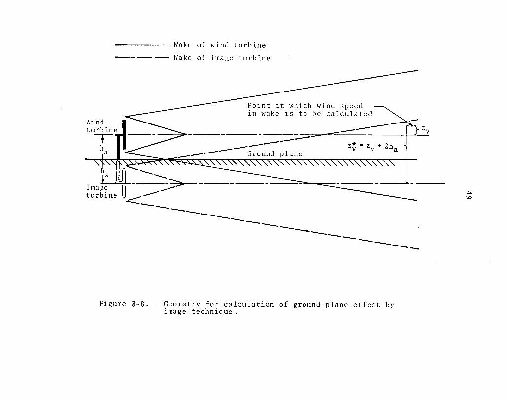
The presence of the turbine at distance, ha' is shown in Figure 3-8. point (y,z), relative to

ground is modeled by placing an image below the ground. The imaging technique Let zv* denote the altitude of the the axis of the image turbine. Then

z * = z+h v a

Using the value of z * instead of z , Subroutine CALCU is called to calculate u*, theVnormalized win~ speed at point (y,z) in the wake of the image turbine. The total wind speed deficit in the wake in ground effect is the sum of the wind speed deficits in the wakes of the real turbine and of the image turbine. If u is the normalized wind speed for a wake in ground effect, thengthe sum of the wind speed deficits is

l-ug = (l-u)+(l-u*)

where th~ 1 is the normalized wind speed of the free stream. Rearranging equation (3-98) gives

u = u+u*-l g

By definition, the approach conserves the total mass deficit. The mass deficit in the real wake is (I-u). The mass deficit

(3-97)

(3-98)

in the wake of the image turbine is (I-u*), and the mass deficit of the wake in ground effect is (I-u). Equation (3-97) shows that the mass deficit for the wake ift ground effect is the sum of the mass deficits for the wakes of the real and image turbines.

It is noted that the presence of the ground does not affect the shape of the wake boundary above the ground. This is shown in Figure 3-9. The only portion of the wake which is affected by the ground effect is that portion of the wake which lies' in the intersection of the wake of the real turbine and the wake of the image turbine.

3.8 Calculation of Wind Speed

For the horizontal wind speed profiles, the input parameter, NP, specifies whether the wind speed is to be normalized by the free stream wind speed at the altitude of the profile or is to be normalized by the free stream wind speed at the hub altitude. If NP = 0, the wind speed in the wake is normalized by the free

34

stream wind speed at the altitude of the wind speed profile. The parameter, u , given by equation (3-98) has been developed as the normalized w~nd speed in the wake in a uniform free stream wind speed. Therefore, u = 1 in the free stream. For a nonuniform free stream wind spe~d profile, if the wind speed in the wake is normalized by the free stream wind speed at the altitude of the wind speed profile, the win~ speed in the free stream is 1. Therefore, u is the wind speed in the wake normalized by the free stream wind ~peed at the altitude of the wind speed profile.

In NP = 1, the wind speed in the wake is normalized by the free stream wind speed at the hub altitude. Then, the wind speed at the altitude of the wind speed profile is

(3-99)

where U (z/h )Y is the free stream wind speed at the altitude of the wind spe~d profile, and (as indicated above) u is the wind speed in the wake normalized by the free stream w~nd speed at the altitude of the profile.

If U has been input in physical units, the graphical output of the pr~gram will be in physical units of wind speed instead of normalized by the free stream wind speed. In this case, the use of NP = 1 will give output in physical units of wind speed for each altitude. The butput for NP = 0 has no desirable interpretation if Uoo i 1.

For the vertical wind speed profile, equation (3-99) is used, regardless of the value of NP or whether the output is normalized by the free stream wind speed or given in physical units. Thus, the wind speed profile of the free stream is always evident on the vertical wind speed profile is y > O.

Table 3-1

FORMAT OF INPUT PARAMETERS FOR TURBINE WAKE COMPUTER PROGRM1

Columns 1-10 11-20 21-30 31-40 41-50 51-60

Card 1 ST CPM AH VHO WEXP RRR

Card 2 J, 10, NP

Card 3 XNPT(l) XNPT(2) XNPT(3) XNPT(4) XNPT(S) XNPT(6)

Card 4 ZO DZZ DYY

Format

6F10.4

312

6F10.4

3F10.4

I

I

VI V1

Symbol

as

m

ha or Ha

U""

y

Table 3-2

TABLE OF INPUT PARAMETERS FOR TURBINE WAKE COMPUTER PROGRAM

Computer Symbol

ST

CPM

AH

VHO

WEXP

Definition

Atmospheric turbulence parameter. If input as a positive number, it is the standard deviation of the wind direction. If input as a negative number, it is the Pasquill stability class as follows:

-1 for Pasquill stability class A -2 for Pasquill stability clas~ B -3 for Pasquill stability class C -4 for Pasquill stability class D -5 for Pasquill stability class E -6 for Pasquill stability class F

If the input value is 0., the wake growth due to ambient turbulence is zero, and the Abramovich wake solution results.

Ratio of free stream wind speed, Uoo ' to the initial wind speed in the wake, UO.

Hub height of the turbine in rotor radii or in physical units as specified by 10.

Ambient wind speed at the hub altitude. If out­put is desired in physical units, input value should be in physical units. If out-put normalized by free stream value is de­sired, input should be 1.0.

Coefficient of the power law profile for the free stream wind speed.

VI 0\

Table 3-2

TABLE OF INPUT PARAMETERS FOR TURBINE WAKE COMPUTER PROGRAM (Continued)

Symbol

Rd

J

10

NP

Xd or Xd

Computer Symbol

RRR

J

10

NP

XNPT(j)

Definition

Rotor radius. An input value of 1.0 will give all output of units of length in rotor radii. An input value of O.S will give all output of units of length in rotor diameters. An input value greater than 2.0 will give all output of units of length in the physical units used for the rotor radius.

Number of downwind locations at which wind speed profiles are to be calculated.

Input option for parameters with physical dimensions of length (AH, XNPT, ZO, DZZ, DYY)

10 = 1 for input in rotor radii 10 = 2 for input in physical units (must be same

physical units as used for rotor radius).

Specifies how velocity is to be normalized for plots of wind speed profiles in the lateral direction.

NP = 0 normalizes wind speed by the free stream wind speed at that altitude

NP = 1 normalizes wind speed by the free stream wind speed at the hub altitude.

Downwind locations at which wind speed profiles are to be calculated (rotor radii or physical units as specified by 10).

(.N

-..:J

Table 3-2

TABLE OF INPUT PARAMTERS FOR TURBINE WAKE COMPUTER PROGRAM (Concluded)

Symbol

Zo or Zo

flz or flZ

fly or flY

Computer Symbol

zo

DZZ

DYY

Definition

Minimum altitude at which wind speed profiles are to be calculated (rotor radii or physical units as specified by 10).

Increment in altitudes at which wind speed profiles are to be calculated (rotor radii or physical units as specified by 10).

Increment in y by which calculations qre to by made in generating the wind speed profiles (rotor radii or physical units as specified by 10).

lM ex:>

Surface wind speed at 10m

(m/sec)

<2

2-3

3-5

5-6

>6

Table 3-3

KEY TO PASQUILL STABILITY CALSSES

Day Night

Incoming solar radiation Thinly overcast or

Strong Moderate Slight ~4/8 Low cloud

A A-B B

A-B B C E B B-C C D

C C-D D D

C D D D

'53/8 Clow::

F

E

D

D VI 1.0

Turbine disk

Initial wake

Far wake

II

RZ1 RZZ Region III

X -I I11III H

R = d R = o R = 1 R = Z RZ1=

XN

Radius of turbine disk

Initial wake radius

Radius of potential core

Outer radius of wake

Outer radius of wake at end of Region I

RZZ = Outer radius of wake at end of Region II

XH = Downwind extent of Region I

XN = Downwind extent of Region II

Figure 3-1. - Wake geometry for the wake computer model.

~ o

41

Read data

Calculate parameters in rotor radii if they have been input in physical units.

Calculate wake growth rate due to ambient turbulence from standard deviation of wind direction or from Pasquill stability class.

Calculate initial wake radius, rO; wake radius at end of Region I , r21; and downwind extent of Region I , xH·

Calculate wake radius at end of Region II, r 22 ; and downwind extent of Region I I, Xw

Save values of wake radius at input values of XNPT(j) for the XNPT(j) which lie in Regions I or II.

Open plot files.

Q Figure 3-2. Flow diagram for wake model computer program.

42

Create data sets for plotting.

Write x, r Z' u, u , P to approprlate ~ile~.

Calculate wake radius at XNPT(j) by linear interpolation and save.

r 2=r 22 LlU =1 c u =l/m c

Call Subroutine R3 to calculate LlU , (dr/dx), and turbine power faEtor.

Calculate total wake growth rate.

Calculate Xl Set r =r I 2 2 Set X=Xl

Figure 3-2. Flow diagram for wake model computer program (continued).

43

Close plot files

Initialize plotter

Make plots of r Z vs. x, ~uc vs. x, and P vs. x.

Open plot files for profile plots.

Generate and plot lateral wind speed profiles. Call Subroutine CALCU to calculate values of wind speed in the wake.

No

Generate and plot vertical wind speed profiles. Call Subroutine CALCU to calculate values of wind speed in the wake.

Close plot files for profile plots.

Figure 3-Z. Flow diagram for wake model computer program (concluded).

44

300

'0 200 /-----f--

100~--+-----/

501----'/0

30

20

10

5~~---r-------+------+------+---------~----~

3L-----L---~~~~~~----~--~~~~~~

.1 .2.3 .5 1 2 3 5 10

Distance downwind from the source (km)

Figure 3-3. Pollution dispersion coefficient as a function of distance downwind of the source.

1.2

1.0

0.8

0.6

0.4

N h o . 2

.......... h

h 0 Q)

+J Q)

S C'j 0.2 h C'j

0..

I/) 0.4 ~

''-;

"0 C'j

0.6 h

Q)

~ C'j

:s: 0.8

1.0

1.2

45

--- Gauss ian wind speed profile

---------Wind speed profile in far wake of present model

deficit parameter, u-u c

u -u 00 c

Figure 3-4. Comparison of the Gaussian wind speed profile used in plume dispersion analysis with the wind speed profile used in the far wake of the wake model.

2

!-<

Free Stream flow

46

~ rO I""'c:::~_ Boundary ~ -----. __ layer OM ______

"d 1 ro !-<

Cl)

,.!:<: ro ~

(a)

o 2 4

Distance downwind of turbine, x Region I for Abramovich solution (no ambient turbulence)

(b) Region I with ambient turbulence

Figure 3-5. ~ Geometry of Region I of the wake for calculating the downwind extent of Region I.

Not to scale

u 00

Wake of upwind turbine

Disk of upwind turbine

I~XPI

Figure 3-6. - Geometry of one turbine centered in the wake of another identical turbine.

Wind speed profile of wake of upwind turbine

Disk of downwind

turbine +:­'-l

1. O.

------.---~

0.8t-

/-~::..:=--~- .-

Ip.. 0/;:/

I-< /Ij

0 .j..J

u /1 m = 3 til ~

I-< .(1) ~ 0 P<

Ii m = 2

/ -m=1.S +>-00

(I)

~ ,,-1

..0 I-< 0.2 ~

E-<

o 2 4 6 8 10 12 14 16 18

Wake radius, R2/Rd

Figure 3-7. - Turbine power factor as a function of wake radius.

-------

Wind turbine ,

h a

Wake of wind turbine

Wake of image turbine

Point at which wind speed ~ in wake is to be calculated ___ ~

--~--::-:: ...... ------------___ ------ Ground plane ---..e-::::: ----:-- r)- zy

z* = z + 2h Y Y a

1 a ~il __:;---=-Image II ...--t u r b i ne -.c::::::::

-------------------------

Figure 3-8. - Geometry for calculation of ground plane effect by image technique.

+:-1.0

50

Wake of real turbine

Portion of wake affected by the ground plane

Ground plane

Wake of image turbine

Figure 3-9. Illustration of the portion of the wake affected by the ground plane.

51

4.0 COMPARISON WITH PREVIOUS MODEL

There are some differences between the model presented in the previous section and the AeroVironment model presented_ in reference 8. For the purpose of completeness, those dif­ferences are documented in this section.

4.1 Wake Growth Rate Due to Ambient Turbulence

For the calculation of wake growth due to ambient tur­bulence, the AeroVironment model uses the expression

ct - o.sr (4 -1)

where ct is a direct data input for the calculation. Methods for determining the value of ,ct were suggested, but not de­tailed. These included evaluating ct from the effective turbulence intensity of the atmosphere at the site, or from the growth rates of smoke or polutant plumes as given in atmospheric dispersion theory. The present model uses the growth rate due to ambient turbulence as

(4 - 2)

where ct is calculated internally from input considerations of Pasquill stability class designation for the atmosphere as given in dispersion theory. This is done in conjunction with the Taylor assumption for the relationship between velocity deficit profile and admixture profile (corresponds to the 1/0.51 in the AeroVironment formulation).

The AeroVironment model has provision for different values for vertical and lateral (normal to the wind direction) com­ponents of wake growth due to ambient turbulence. Under these conditions, the wake (out of ground effect) assumes an ellip­tical cross section instead of a circular cross section. This condition was not included in the present version for sim­plicity and because of the uncertainty about the appropriate procedure for relating unequal wake growth rates to an axisym­metric flow solution. In the present model, the wake growth rate due to ambient turbulence was taken as the lateral growth rate.

52

4.2 Support Tower

The effect of the wake of the turbine support tower was not included in the present version because it was believed to be an unwarranted complexity. Tower wake relationships de­pend on the type of construction (i.e., lattice or tubular) and the interaction between the tower wake and the turbine wake. Furtherfore, the effects of the tower wake should be diminished in the far wake of the turbine, which is the prin­cipal region of interest. Thus, the tower wake effect was deemed negligible compared to the other uncertainties in the model formulation.

4.3 Calculations for Region I

The calculation of r 21 , the wake radius at the end of Region I was done differently in the revised model than in the AeroVironment model. The AeroVironment model used equation (5.21'.) of Abramovich. At the end of Region I, the boundary layer width, b, is r 21 • In Abramovich's notation, y is the distance from the inltial wake radius to the boundary of the potential core. Therefore, at the end of Region I, Yl = rO' and equation (5.21') of Abramovich can be written as

r 21 = O.416+0.134m+O.021---(1+0.8m-O.45m2) (4-3)

rO

This is a quadratic equation in r21 /rO which is solved for r Zl /rO to give

r 21 -f+I£2+4g = (4-4)

Zg

where

f = O.416+0.134m (4-5)

g = O.OZl(1+0.8m-O.45m 2) (4-6)

The positive sign was chosen for the solution to the quadratic equation so that r 21/rO is positive.

53

Although this approach is correct, it was deemed to be unnecessarily cumbersome. The parameter, r 2l /rO is given directly by Abramovich, equation (5.19) as

ro r 2l

= 10.2l4+0.l44m (4-7)

This equation (same as eq. (3-34) was deemed to be simpler than that presented in the AeroVironment model. Numerically, the difference between these two methods is less than 0.4% for values of m between 1 and 3.

In the AeroVironment model, only one approach for calculating the downwind extent of Region I was presented. This was the first approach (r l approach) described in Appendix D. After consideration of this approach, it was realized that the second approach (r 2 approach) described in Appendix D was equally plausible from a physical phenomenological point of view, but the r approach gave much different results. This paradox prompted the investigation of other approaches, and the seven approaches outlined in Appendix D resulted. The approach which was eventually chosen was not the approach originally pre-sented in the AeroVironment model. The reader is referred to Appendix D for the description of the AeroVironment ap-proach and the six other approaches considered.

4.4 Wake Growth in Region III

The AeroVironment model attempted to simplify the calculation of wake growth in Region III in order to circum-vent the necessity of the numerical integration in Region III. The basic idea by which the calculation procedure was to be simplified was to perform the numerical integration externally to the wake program for different sets of values of a and m. ' The numerical integrati~n was performed over an interval of x of 10rO beginning with the wake radius r 22 , which is a function of m only. Once the wake radius was known at the beginning and end of Region III, the effective ambient turbulence was defined as that ambient turbulence which alone would give the same wake growth in Region III as the combination of mechanical turbulence and ambient turbulence had given in Region III by the numerical integration. For example, for m = 3 and a = 0.1,

rO = 1.414 (4-8)

r 22 = 1.988 (4-9)

xN = 5.488 (4-10)

54

The downwind extent of Region III is 10rO or at

x = xN+lOr O = 19.63 (4-11)

From the numerical integra~ion of equations (3-57) through (3-62), r 2 = 3.43 at x = 18.42, and r 2 = 3.57 at x = 19.83. By linear interpolation, r 2 = 3.55 at x = 19.63. Therefore, in Region III

(dr2) 3.55-1.99

a e = dx avg = 19.83-5.49 = 0.1088 (4-12)

Therefore, for m = 3 and a = 0.1, the effective growth rate in Region III is a e = 0.1088.

In the AeroVironment model, the numerical ingetration was conducted external to the main wake computer program. Plots of a e as a function of a were generated for several selected values of m, and ap' was an input paramter for the wake computer program. In Region III, the wake growth rate was assumed to be constant at a value of a. In Region IV (downwind of Region III), the wake growth rate w~s assumed to be constant at a value of a. That is, downwind of x = xN+lOrO' the wake growth was assumed to be due to ambient turbulence alone with no contribution to wake growth due to mechanical turbulence. In this discussion, the definition of a used in this report is the growth rate of the wake radius due to ambient turbulence. In the AeroVironment report, a was defined slightly differently, and the growth rate of the wake radius due to ambient turbulence is shown in the AeroVironment report as a/0.5l.

The method used in the AeroVironment report is reasonably accurate, acsept for low values of ambient turbulence. At low values of ambient turbulence (a<O.l), there is still a sig­nificant value of wake growth due to mechanical turbulence down­wind of x = xN+lOrO. Also, it was deemed appropriate that the model should assume the exact form of the Abramovich solution for a = O. The AeroVironment model does not do that since the wake growth rate in Region IV goes to zero for a = O. For these reasons, in the revised model, the numerical integration of equations (3-57) through (3-62) was made an integral part of the model.

55

5.0 SAMPLE PLOTS

This section contains sample plots made with the turbine wake computer program. The plots were made from seventeen runs of the program. Illustrated in this section are the in­put of parameters for the computer program and the output ob­tained. The first part of this section presents complete sets of plots from the computer program. These figures include plots of the Abramovich solutions (i.e., no ambient turbulence). The second part of this section shows the effect of changes in wake variables on wake recovery. Results are presented for changes in ambient turbulence factor; power law exponent, height of the axis of the turbine rotor, and initial veloc-ity ratio.

5.1 Wake Plots

Abramovich solutions. - Initially, it was desired to ob­tain plots for the Abramovich solution for the coflowing jet (a = 0). The input parameters ,are shown below.

VALUES OF INPUT PARAMETERS FOR TURBINE WAKE PLOTS FOR ABRAMOVICH SOLUTION

ST = 0.0 J = 5

CPM = 1.5 10 = 1

AH = 50. NP = 0 VHO = 1.0 XNPT = 5., 10" 2 0., 35., 50. WEXP = O. ZO = 48.5

RRR = 1.0 DZZ = 0.5 DYY = 0.05

The input value, ST = 0.0, makes the ambient turbulence zero. The value of CPM = 1.5 was chosen as a typical value. for large wind turbines. The value AH = 50. was used to make the wake isolated from the ground effect. VHO = 1.was used to make all wind speed plots normalized by the free stream wind speed. The power law exponent, WEXP = ~ gives no variation in free stream wind speed with altitude. The rotor radius, RRR = 1.0 gives all geometric output in rotor radii. J = ~ indicates five downwind locations at which wind speed proflles are to be calculated. 10 = 1 indicates that geomteric input

56

is in rotor radii. NP = a indicates that the wind speed profiles are to be normalized by the free stream wind speed at the altitude of the profile. The values of downwind location at which wind speed profiles are to be generated are defined by XNPT (j) = 5:, 10., 20., 35" and 50.. For the wind speed profiles, ZO = 48.5, and DZZ = 0.5. The altitudes at which the wind speed profiles are to be calculated are

i=O, ... ,7 (5 -1)

Therefore, the altitudes of the lateral wind speed profiles are 48.5, 49.0, 49.5, 50.0, 50.5, 51.0, 51.5, and 52.0. Since h = SO. for the input values of zo and ~z, the fourth wind s~eed prDfile is at the hub altitude. The second wind speed profile is at the lower edge of the turbine disk, and the sixth wind speed profile is at the upper edge of the turbine disk. The value, DYY = 0.05, indicates that calculations are made at intervals of 0.05 rotor radii.

Figure 5-1 shows the set of computer-generated plots for the set of input data shown in the preceding table. The first plot shows the wake radius and the wake width as a function of the downwind coordinate, x. Since the wake is not near the ground, the wake height above the ground is not shown. The first plot also lists the important wake parameters for the set of plots. The second plot shows 6uc as a function of x, and the third plot shows Uc/U as a function of x. The fourth plot shows the variation of turbine power factor. Since the turbine power factor is undefined in Regions I and II, the plot is shown downwind of xN only. The fifth through the ninth plots show the lateral wind speed profiles for the down­wind locations shown in the table. The altitude of each pro­file is shown in rotor radii relative to the turbine hub. Since the wake is far from the ground, the vertical wind speed profile at y = 0 is symmetrical to the lateral profile at Zv = Rd' It wa~ therefore, not shown.

Figure 5-2 shows a set of similar plots for m = 2.0, and figure 5-3 shows the values for m = 3.0. The first plots of each of figures 5-1, 5-2, and 5-3 is similar to the plots given by Abramovich in figure 5.17 of reference 2. The second plot in each of these figures is similar to figure 5.20 in refer­ence 2. In the Abramovich plots, the geometric parameters are normalized by the initial wake radius, RO' In figures 5-1, 5-2, and 5-3, the geometric parameters are normalized by the turbine dish radius, Rd' The relationship between RO and Rd is given by equation (3-18).

57

Wakes in ground effect. - The input parameters for the wake in ground effect are listed below. The hub of the tur­bine is 1.35 rotor radii above the ground. This is typical of very large wind turbines. The first lateral wind speed pro­file (i = 0; zO = 0.35) is at the lower edge of the turbine disk, and the third lateral wind speed profile (i = 2) is at the rotor hub.

VALUES OF INPUT PARAMETERS FOR TURBINE WAKE PLOTS FOR WAKE IN GROUND EFFECT

ST = 0.0 CPM = 1. 5 AH = 1. 35

VHO = 1. 0

WEXP = 0.15 RRR = 1. 0

J = 5

10 = 1

NP = 0

XNPT (j) = 5., 10., 20., 35., 50. ZO = 0.35 DZZ = 0.5 DYY = 0.05

Figure 5-4 shows the set of wake plots for the input data shown above. Since the wake is near the ground, the height of the top of the wake above the ground is also shown in the first plot, and a vertical wind speed profile plot is included. In the plot of the vertical wind speed profiles, the solid line going across the plot is the wake center. The short horizontal lines at the left of the plot are the bottom and top of the turbine disk.

In the plot of the normalized wake boundaries (Fig. 5-4(1)), the point at which the wake radius equals h , the height of the rotor hub above the ground, is the point atawhich the wake intersects the ground plane. Initially, the effect of the ground plane affects only the lower part of the wake, but it can spread to affect the wake center, although the magnitude of the effect at the wake center is negligibly small because of the l~rge wake radius (and correspondingly small wid speed deficit) necessary for the effect of the ground plane to reach the wake center. It is recalled from the development of the turbine power factor that the turbine power factor does not include the effect ot the ground plane.

58

The effect of the ground on the wind speed profiles is seen by comparing the wind speed profiles for x = 50 from Figures 5-1 and 5-4. In Figure 5-1, the profiles for altitudes of -1.0 and 1.0 rotor radii from the rotor hub are identical because of the symmetry of the wake. However, because of the ground effect, the wind speed profiles at altitudes of -1.0 and 1.0 rotor radii relative to the hub are not identical in Figure 5-4. The lower altitude exhibits a lower wind speed in the wake because of the ground effect. At x = 50, it is only the lowest altitude which has been affected by the ground. As the wake expands further, the effect of the ground affects the wind speed profiles of higher altitudes. This is seen in later plots where ambient turbulence causes faster expansion of the wake.

For all of the previous figures, there is no ambient turbulence. Figure 5-5 shows a plot set for ambient turbulence represented by Pasquill stability class E. The data input is identical with that shown in the table, except that ST = -5. for Pasquill stability class E. From Table 3-4 arid equation (3-28), the wake growth rate due to ambient turbulence is a = 0.099.

Figure 5-6 shows a plot set for Pasquill stability class D (ST = -4J. The wake growth rate due to ambient turbulence is a = 0.136. Figure 5-7 shows a plot set for Pasquill sta­bility class C (ST = -3J. The wake growth rate due to ambient turbulence is a = 0.205.

5.2 Effect of Principal Wake Parameters In the following discussion, the effect of the principal

wake parameters upon the wake is investigated. The parameters which are varied are the ambient turbulence as represented by the Pasquill stability class; the initial velocity ratio, m; the height of the rotor hub, ha ; and the power law coefficient of the free stream wind speed profile, y.

Effect of ambient turbulence. - Figure 5-8 shows the effect of amblent turbulence on the wake radius. Figure 5-8 is a composite of the wake radius as shown in the first plot of Figures 5-4 through 5-7. Figure 5-9 shows the effect of ambient turbulence of ~u~. Figure 5-10 shows the effect of ambient turbulence on Uc/Uoo • Figure 5-11 shows the effect of ambient turbulence on the turbine power factor. It is seen that ambient turbulence is a very important factor in the recovery of wakes of large wind turbines. From Table 3-3, it is recalled that most turbine operation occurs with Pasqui1l stability class D, and Pasqui11 class D represents the ambient turbulence level to which inter-turbine spacing should be designed.

59

The turbine power factor is the most significant indicator of wake recovery. From Figure 5-11, for Pasquill stability class D, the turbine power factor is approximately 0.9 at a distance of 35 rotor radii downwind of the turbine. While the ambient turbulence has a significant impact on the growth in the wake radius, its impact on the turbine power factor is not great. For comparison with the 0.90 power factor for Pasquill stability class D, the turbine power factor is 0.85 for Pasquill stability class E and 0.95 for Pasquill stability class C at 35 rotor radii downwind of the turbine.

It is clear that a point of diminishing returns is reached in the re-energization of the turbine wake. From Figure 3-7, for m = 1.5, a turbine power factor of 0.9 is reached at r 2 ~ 5.4 Figures 5-8 and 5-11 confirm this number since Figure 5-11 shows that P = 0.9 at approximately x = 34 for Pasquill stability class D, and Figure 5 - 8 shows that r 2 = 5 .4 at x = 34 for Pasqui1l stability clas~ D. From Figure 3-7, the turbine power factor reaches a value of 0 .. 9 .5 at wake radius, r 2 ~ 8. From extrap-01ation of the wake radius for Pasquill stability class D in Figure 5-8, a wake radius of 8 occurs at x ~ 56. Thus, a distance of 35 wake radii is required for recovery from the initial wake to a turbine power factor of 0.9, and an additional distance of 21 rotor radii is required for recovery from 0.90 to 0.95 for the turbine power factor. Certainly, power recovery is very much slower after the turbine power factor reaches 0.9 than it is before it reaches 0.9.

For the far wake, Figure 3-7 is essentially a plot of turbine power factor as a function of downwind distance since the wake radius is a straight line function of the downwind coordinate, x. In the far wake, the wake growth rate is alm.ost entirely due to ambient turbulence with very little contribution from mechanical turbulence. For Pasquill stability class D, a scaling factor of 1/0.136 should be applied to the wake radius axis of Figure 3-7 ~o convert it to distance downwind of the turbine, since the wake growth rate due to ambient turbulence is 0.136 for Pasquill stability class D. Interpreting Figure 3-7 in this way shows that a very large downwind distance is required for recovery of the last few percentage points for the turbine power factor. In practice, recovery to very high values of turbine power factor may be im­practical because of the large additional distances required.

Effect of initial velocity ratio. - Figure 5-12 shows the effect of the initial velocity ratio, m, upon the wake radius. Figure 5-13 shows the effect of m upon ~uc. Figure 5-14 shows the effect of m upon Uc/U~, and Figure 5-15 shows the effect of m upon the turbine power factor.

60

The initial velocity ratio has almost no effect upon the wake radius. The downwind extent of Region II, XN, is almost totally unaffected by m. This is shown in Figures 5-13, 5-14, and 5-15. Figure 5-13 shows the relative wind speed deficit (i.e., the wind speed deficit at the wake center normalized'by the wind speed deficit at the center of the initial wake). This relative wind speed deficit is not a strong function of m. However, because the wind speed deficit of the initial wake is much larger for a large value of m (by definition of m), the normalized wind speed at the wake center (as shown in Figure 5-14) strongly depends on m. Correspondinge1y, the turbine power factor shown in Figure 5-15 is a strong function of m. For the larger values of m, more power is extracted by each wind turbine (cf. equations (3-9) and 3-11)), but the inter-turbine recovery of the wake requires more space. The lines shown in Figure 5-15 approximate the cube of the lines shown in Figure 5~14.

Effect of turbine rotor height. - The wind sp~ed profile plots are the only plots which show the effect of the ground on the wake. The ground effect can be seen best from the vertical wind speed profiles with y = 0 (i.e., no variation in the free stream wind speed with altitude). Figures 5-16, 5-17, and 5-18 show the vertical wind speed profiles for values of ha of 1.2, 1.35, and 1.65, respectively.

In the near wake (x = 5 and x = 10), the wake is approximately symmetric for h = 1.35 and h = 1.65. For the far wake (x = 20, x = 35,aand x = 50) tfle wake is clearly not symmetric for all values of h. The effect of the ground upon the wind speed profiles can Be clearly seen by comparing the profiles for x = 20 from the three plots. The retarding effect of the ground is clearly evident. For comparison, Figures 5-19, 5-20, and 5-21 show the same data as Figures 5-16, 5-17, and 5-18, but with a power law coefficient, y, of 0.15.

Effect of the ¥ower law coefficient. - The power law exponent, y, only a fects the vertical wind speed profile. It can be seen on the vertical wind speed profile and on the lateral wind speed profile (if NP = 1 so that the wind speed in the wake is normalized by the free stream wind speed at the hub altitude). The effect of y on the vertical wind speed profile may be seen by comparing Figures 5-13, 5-20, and 5-22. The value, y = 0.25 in Figure 5-22 represents a very turbulent lower atmosphere.

61

(1). NORMALIZED WAKE BOUNDARIES

No ambient turbulence P::o m=1.5 !zJ cr) h = 50. (no ground effect) tl ya= 0.0 ::s <0 P::d

0: >q P::. < Q Z Wake width ::>0 Orl ~

~ ::'::0

~(\fL ____ ~:------Wake radius

9

~ +---~r---~----~----~--~----~----~--~----~--~ 0.0 ~ ~ ~ ~ ~ ~ ~ ~ ~ 60.0

DISTANCE DOWNWIND FROU TURBINE I X/Rd

Figure 5-1. Wake plots for Abramovich solution for m = 1.5.

-o

62

(2). NORMALIZED WIND SPEED DEFICIT AT THE WAKE CENTER ::>0

I ~~------------------------------------------___ 8 ::> ...-"­o~ ::> ,

8 e~ E--...... U ...... ~ f!jd Q

~~ tzl p.. rn Q8+---~----~--~----~---r----~--~--~----~--~ ~ 0.0 ~

~ ~ ~ ~ ~ ~ ~ ~ ~ ~

DISTANCE DOWNWIND FROU TURBINE. X/Rd

Figure 5-1. Wake plots for Abramovich solution for m = 1.5 (continued).

63

(3). NORMALIZED WIND SPEED AT THE WAKE CENTER

M ~ ~ ~ ~ ~ ~ ~ ~ ~

DISTANCE DOWNWIND FROM TURBINE I X/Rei

Figure 5-1. Wake plots for Abramovich solution for m = 1.5 (continued).

8~ 0..

" 0..

~~ 0 E-< U ~.

d O! ~

~~

~ 0.0 ~.O

64

(4). TURBINE POWER FACTOR FOR AN UNBOUNDED WAKE

-----

~ ~ ~ ~ .~ ~ ~ ~ ~

DISTANCE DOWNWIND FROU TURBINE I X/Rd

Figure 5-1. Wake plots for Abramovich solution for m = 1.5 (continued).

65

( 5). LATERAL WIND SPEED PROFILE

AT X/Rd = 5.00

Altitude of wind speed profile in rotor radii relative to the wake center

-1.5, 1.5, 2.0

g~~r-~r-----------------------------

8 ~CQ "",",0 ~

0' ~~ til ° ~ rIJ

O~ :Z;o ~

~

o

-1.0, 1.0

-0.5, 0.5

o.

oj-----Ir-----r-----.----~----~----~ 0.0 1.0 2.0 S.O 4.0 5.0 6.0

LATERAL COORDINATE t Y/Rd

Figure 5-1. Wake plots for Abramovichsolution for m = 1.5 (continued).

66

( 6). LATERAL WIND SPEED PROFILE

AT X/Rd = 10.00

-1.5, 1.5, 2.0

9~~~-n--------------------------

8 ::Jeq ",,",0 ::::>

o ~~ CilO ~ en ~~ Z;o ... ~

q

0.0

1.0

0.5

O~----r---~----~----~--~----_ 0.0 1.0 2.0 5.0 '.0 5.0 6.0

LATERAL COORDINATE , Y/Rd

Figure 5-1. Wake plots for Abramovich solution for m = 1.5 (continued).

67

( 7). LATERAL WIND SPEED PROFILE

AT X/Rd = 20.00

-1.5, 1.5, 2.0

3~~--~~------------------------

8 ~CQ '-..0 ~

d' ~~ w o ~ OJ

A~ ZO ...... ~

1.0

-0.5, 0.5

0.0

g~----~--~----~----------~--~ 0.0 1.0 2.0 5.0 4.0 5.0 6.0

LATERAL COORDINATE . Y/Rd

Figure 5-1. Wake plots for Abramovich solution for m = 1.5 (continued).

68

( 8). LATERAL WIND SPEED PROFILE

AT X/Rd = 35.00

2.0

94-~~~ __ -----------------------

8 ~cq ,",c ~

ci ~~ r:a o 0.. rn ~. Zd ...... ~

" . '---1.5, 1.5

~ -1.0, 1.0

-0.5, 0.5

0.0

~4-----r---~----~----'---~----1 0.0 1.0 ao 5.0 4.0 6.0 e.o

LATERAL COORDINATE t Y/Rd

Figure 5-1. Wake plots for Abramovich solution for m = 1.5 (continued).

C\l """'

q -8

~CQ "",,0 ~

0-r.:I~ [J:Jo 0.. rn o. Zo ...... ~

~ Q

q

69

( 9). LATERAL WIND SPEED PROFILE

AT X/Rd = 50.00

2.0

1.5

1.0

0.5

0.0

Q+-----~--~----~----~--~----~ 0.0 1.0 2.0 5.0 4.0 5.0 6.0

LATERAL COORDINATE , Y/Rd

Figure 5-1. Wake plots for Abramovich solution for m = 1.5 (concluded).

~

~ ~~ tl ~ 4(

~~ < g..

>-q ~~ < Q Z :Ja o~ ~

frJ

~~

9

~

70

(1). NORMALIZED WAKE BOUNDARIES

No ambient turbulence m = 2.0 ha = 50. (no ground effect) y = 0.0

~ __ -------~w~ake radius

0.0 e.G ~ ~ ~ ~ ~ ~ ~ ~ ~

DISl'ANCE DOWNWIND FROY TURBINE'. X/Rei

Figure 5-2. Wake plots for Abramovich solution for m = 2.0.

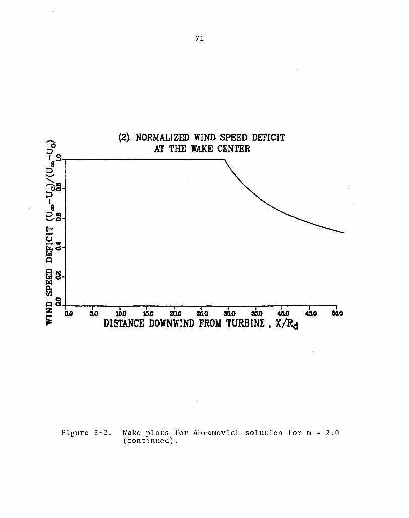
-o

71

(2). NORMALIZED WIND SPEED DEFICIT AT THE WAKE CENTER 79 8 ~------------------~----~

::> -~~ ::> I 8 2.~ E-t -U -~ f:i Q

~~ r&l 114 Ul

Q~+---~--~----r---~--~--~~--~--~--~--~ :: 0.0 ~

~ ~ ~ ~ ~ ~ ~ ~ ~ ~

DISTANCE DOWNWIND FROM TURBINE I XIRci

Figure 5-2. Wake plots for Abramovich solution for m = 2.0 (continued).

72

(3). NORMALIZED WI ND SPEED AT THE WAKE CENTER

~ ~ ~ ~ ~ ~ ~ ~ ~ ~

DISI'ANCE DOWNWIND FROM TURBINE I X/Rci

Figure 5-2. Wake plots for Abramovich solution for m = 2.0 (continued) .

9

~~ "-~

~~

~ ~~

d 0:: ral

~~ ~

0.0 0.0

73

(4). TURBINE POWER FACTOR FOR AN UNBOUNDED WAKE

~ ~ ~ ~ ~ ~ ~ ~ ~

DI5TANCE DOWNWIND FROM TURBINE I X/Rei

Figure 5-2. Wake plots for Abramovich solution for m = 2.0 (continued).

74

( 5). LATERAL WIND SPEED PROFILE

AT X/Rd = 5.00

Altitude of wind speed profile in rotor radii relative to the wake center -1.5, 1.5, 2.0

q ... 8

Ocq '-..Q ~

.. 1.0 0 ~"'! ~o 0.5 ~ (f)

O~ 0.0

Zd .... ~

~ 0

~4-----~----~----~----~----~--~ 0.0 LO 2.0 5.0 "'.0 6.0 6.0

LATERAL COORDINATE t Y/Rd

Figure 5-2. Wake plots for Abramovich solution for m = 2.0 (continued) .

q ~

8 OCQ '-..,0 ~

.. 0 ~CD ~o 0... rn 0 ... Zd -~

cq 0

75

( 6). LA'1ERAL WIND SPEED PROFILE

AT X/Rd = 10.00

-1.5, 1.5, 2.0

-0.5, 0.5

0.0

~4-----~--~----__ --__ ----~--___ 0.0 10 2.0 5.0 '.0 6.0 8.0

LA7ERAL COORDINATE t Y/Rd

Figure 5-2. Wake plots for Abramovich solution for m = 2.0 (continued) .

8 Ocq ",,0 ::J

ci ~cc. ~o 0., OJ

o. Zc ~

~

~ 0

76

( 7). LATERAL WIND SPEED PROFILE

AT X/Rd = 20.00

1.5

0.5

0.0

~~--------~--------~~---r--___ 0.0 to 2.0 9.0 '.0 5.0 5.0

Figure 5-2.

LATERAL COORDINATE t Y/Rd

wcake plots for Abramovich solution for m ~ 2,0 continued) .

q -8

OCQ ,",0 !:)

.. 0 ~~ CxJo 0-C/)

o. Zd ~

~

cq 0

77

( 8). LATERAL WIND SPEED PROFILE

AT X/Rd = 35.00

1.5

1.0

- 0 . 5, 0.5

0.0

~~--~~--~--------~----~----0.0 1.0 aD 5.0 4.0 6.0 8.0

LA'IERAL COORDINATE t Y/Rd

Figure 5-2. Wake plots for Abramovich solution for m = 2.0 (continued).

78

( 9). LATERAL WIND SPEED PROFILE

AT X/Rd = 50.00

2.0

9 L-~--~~~--------------------

8 ::>cq '-..0 !::>

ci ~~ r:.JO 0., rn ~~ Zo ...... ~

-1.5, 1.5

-1.0, 1.0

-0.5, 0.5

0.0

~~--~~--~--------~----~----0.0 to 2.0 S.O 4.0 5.0 8.0

Figure 5-2.

LATERAL COORDINATE , Y/Rd

Wake plots for Abramovich solution for m = 2.0 (concluded).

9

79

(1). NORMALIZED WAKE BOUNDARIES

No ambient turbulence m = 2.5 ha = 50. (no ground effect) y = 0.0

Wake width

Wake radius

~+---~--~--~--~--~--~--~---r--~--~ ~ ~ ~ ~ ~ ~ ~ ~ ~ ~ ~

DISTANCE DOWNWIND FROY TURBINE I X/Rei

Figure 5-3. Wake plots for Abramovich solution for m = 2.5.

'0

80

(2). NORMALIZED WIND SPEED DEFICIT AT THE WAKE CENTER 10

8~~--------------------~

2-~~ :J ,

8 2.~ E---~ ... tid Q

~ ~ ~ ~ ~ ~ ~ ~ ~ ~

DISI'ANCE DOWNWIND FROM TURBINE I X/Rei

Figure 5-3. Wake plots for Abramovich solution for m = 2.5 (continued).

81

(3). NORMAIJZED WIND SPEED AT THE WAKE CENTER

~ ~ ~ ~ ~ ~ ~ ~ ~ ~

DISfANCE DOWNWIND FROM TURBINE I X/Rd

Figure 5-3. Wake plots for Abramovich solution for m = 2.5. (continued) .

82

(4). TURBINE POWER FACTOR FOR AN UNBOUNDED WAKE

~+---~----~--~--~~--~--~----~--~--~--~ ~ ~ ~ ~ ~ ~ ~ ~ ~ ~ ~

DISTANCE DOWNWIND FROM TURBINE. X/Rd

Figure 5-3. Wake plots for Abramovich solution for m = 2.5 (continued) .

83

( 5). LATERAL WIND SPEED PROFILE

AT X/Rd = 5.00

Altitude of wind speed profile in rotor radii relative to the wake center -1.5, 1.5, 2.0

9;-~---r~---------------------------

8 :Jeq '-..0 ~

o ~~ ril° ~ tr.}

~.

-1.0, 1.0

0.5

0.0 Z C -+-_--J.-' -~

~4-----~----~----~----~----'-----' 0.0 1.0 2.0 5.0 4.0 6.0 6.0

LATERAL COORDINATE t Y/Rd

Figure 5-3. Wake plots for Abramovich solution for m = 2.5 (continued) .

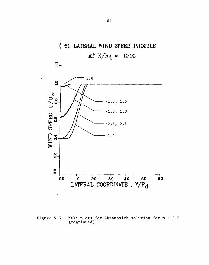
8 ~CQ ,,"0 ~

~~ Zo -~ ~ 0

84

( 6). LATERAL WIND SPEED PROFILE

AT X/Rd = 10.00

~-2.0

-1. 5, 1.5

1.0

0.5

0.0

~~----r---~----~----r---~----~ 0.0 to 2.0 5.0 4.0 6.0 8.0

LATERAL COORDINATE t Y/Rd

Figure 5-3. Wake plots for Abramovich solution for m = 2.S (continued) .

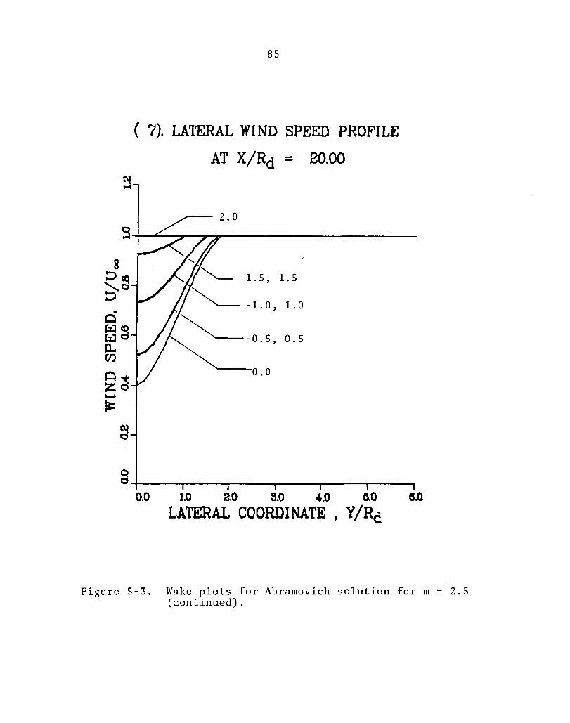
8 O&q '0 !:)

.. Q ~CQ CiJo D., OJ

o. Zd ..... ~

~

85

( 7). LATERAL WIND SPEED PROFILE

AT X/Rd = 20.00

.-- 2.0

1.0

0.5

0.0

~~----~--~----~----~--~----~ 0.0 1.0 2.0 5.0 4.0 ~O 8.0

LATERAL COORDINATE t Y/Rd

Figure 5-3. Wake plots for Abramovich solution for m = 2.5 (continued) .

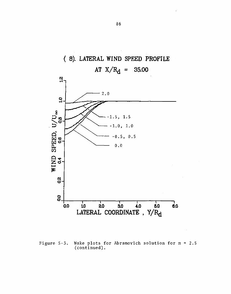
86

( 8). LATERAL WIND SPEED PROFILE

AT X/Rd = 35.00

--2.0

1.0

0.5

0.0

g~---~--~----~--~----~----0.0 LO ao 5.0 '.0 6.0 6.0

LATERAL COORDINATE , Y/Rd

Figure 5-3. Wake plots for Abramovich solution for m = 2.5 (continued).

8 ~CQ '-..0 ::J

d' r::I~ t:rJo ~ en O~ Zd ..... ~

87

( 9). LATERAL WIND SPEED PROFILE

AT X/Rd - 50.00

1.5

1.0

'----0.5, 0.5

0.0

~~----~--~----~----~--~----~ 0.0 10 2.0 5.0 '.0 5.0 6.0

LA1'ERAL COORDINATE t Y/Rd

Figure 5-3. Wake plots for Abramovich solution for m = 2.5 (concluded) .

~o. tlCD ::s <0 ~d

0: ~~ < Q

88

(1). NORMALIZED WAKE BOUNDARIES

No ambient turbulence m = 1. 5

ha = 1. 35

Y = 0.15

Wake width z

~~I ___ --~~--~~~~::::~~::::~-------- L Wake height ~

~ ~ L_---------~--liw;;;akk;-;er;,a~d~i:u:S ----

9

~+-----~---r----~---'----~----r---~----.----'----, ~ ~ ~ ~ ~ ~ ~ ~ ~ ~ ~

DISTANCE DOWNWIND FROll TURBINE I X/Rd

Figure 5-4. Wake plots for wake in ground effect with no ambient turbulence.

-o

89

(2). NORMALIZED WIND SPEED DEFICIT AT THE JAKE CENTER ::>0 I ~~ __________________________________________ ~

8 :> --," -Iq :>t>O I 8 e.~

~ ~ ~ ~ ~ ~ ~ ~ ~ ~

DISTANCE DOWNWIND FROM TURBINE. X/Ret

Figure 5-4. Wake plots for wake in ground effect with no ambient turbulence (continued).

90

(3). NORMAUZED WIND SPEED AT THE WAKE CENTER

~ ~ ~ ~ ~ ~ ~ ~ ~ ~

DISTANCE DOWNWIND FROY TURBINE I X/Ret

Figure 5-4. Wake plots for wake in ground effect with no ambient turbulence (continued).

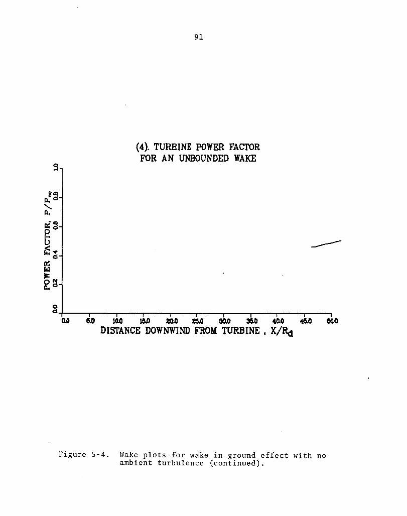
8~ 0.. "-0..

-cq P:::o

~ ~.

d n:: ia:l ~

~~

~ 0.0 ~

91

(4). TURBINE POWER FACTOR FOR AN UNBOUNDED WAKE

----~ ~ ~ ~ ~ ~ ~ ~ ~

DISTANCE DOWNWIND FROM TURBINE. X/Rei

Figure 5-4. Wake plots for wake in ground effect with no ambient turbulence (continued).

92

( 5). LATERAL WIND SPEED PROFILE

AT X/Rd = 5.00

Altitude of wind speed profile in rotor radii relative to the wake center 1.5, 2.0, 2.5

q -8

Oeq 1.0 '-..0

!:) . 0.5

Q ~cc. ~o

0.0

0.. C1J

~ .. Zd ..... ~

~

~4-----~----~----~----~-----r----~ 0.0 to 2.0 5.0 4.0 6.0 8.0

LATERAL COORDINATE , Y/Rd

Figure 5-4. Wake plots for wake in ground effect with no ambient turbulence (continued).

q -8

::J~ ,",0 ~

.. 0 ~CD. CxJo ~ en ~. Zo ...... ~

C\l 0

93

( 6). LATERAL WIND SPEED PROFILE

AT X/Rd = 10.00

,--- 1. 5, 2. 0, 2. 5

1.0

0.5

0.0

~4-----~--~----~----~----~--~ 0.0 to 2.0 S.O 4.0 5.0 8.0

LATERAL COORDINATE , Y/Rd

Figure 5-4. Wake plots for wake in ground effect with no ambient turbulence (continued).

94

( 7). LATERAL WIND SPEED PROFILE

AT X/Rd = 20.00

-- 1.5, 2.0, 2.5

94-~--____ ------------------------

8 O~ '-..c ::> 0' J:z:I~ (:a 0 ~ rn O~ Zc ~

~

0.5

0.0

~~----~--~~--------~----~--~ 0.0 1.0 2.0 5.0 '.0 6.0 8.0

LATERAL COORDINATE , Y/Rd

Figure 5-4. Wake plots for wake in ground effect with no ambient turbulence (continued).

95

( B). LATERAL WIND SPEED PROFILE

AT X/Rd = 35.00

2.0, 2.5

S4-~~--~ __ ----------------------

1.0

0.5

0.0

g~----~--~~--~-----r----~--~ 0.0 to 2.0 5.0 '.0 0.0 6.0

LATERAL COORDINATE t Y/Rd

Figure 5-4. Wake plots for wake in ground effect with no ambient turbulence (continued).

96

( 9). LATERAL WIND SPEED PROFILE

AT X/Rd = 50.00

2.0, 2.5

s~~--~~~----------------------

8 Ocq '0 !:J

ci ~~ ~o c.. CfJ

~. Zd ... ~

-1.0

-0.5, 0.5

0.0

~~----r---~----~----'-----~--~ 0.0 10 2.0 5.0 '.0 6.0 8.0

LATERAL COORDINATE, Y/Rd

Figure 5-4. Wake plots for wake in ground effect with no ambient turbulence (continued).

97

(10). VERTICAL WIND SPEED PROFILES AT WAKE CENTER

Distance downwind of the turbine in rotor radii

50. -----.,.

35. --

20.

10. 5.

0. O~ ____ ~ ____ .. ====~~=-__ ~ ____ ~ __ --.

0.0 0.2 0.4 0.6 0.8 10 1.2 WIND SPEED, U/Uoo

Figure 5-4. Wake plots for wake in ground effect with no ambient turbulence (concluded).

98

(1). NORMALIZED WAKE BOUNDAR I

Ambient turbulence represented by Pasquill stability class E

m = 1. 5

ha = 1. 35

Y = 0.15

Wake width

• .0 5.0 laD 15.0 20.0 260 50.0 56.0 40.0 DISTANCE DOWNWIND FROM TURBINE t X/Rd

Figure 5-5. Wake plots for wake in ground effect for Pasquill stability class E.

-

99

(2). NORMALIZED 'WIND SPEED DEFICIT AT THE WAKE CENTER ";:)0

19~-----"""'\ .J -""-o~ ";:) I 8 e~ E--U. fi:d I'a:J ~

~~

~ Q~+-------~--------------------------~--------Z -• 0.0 &.0 10.0 16.0 20.0 ao 30.0 36D 40.0

DISTANCE DOWNWIND FROM TURBINE • X/Rd

Figure 5-5. Wake plots for wake in ground effect for Pasquill stability class E (continued).

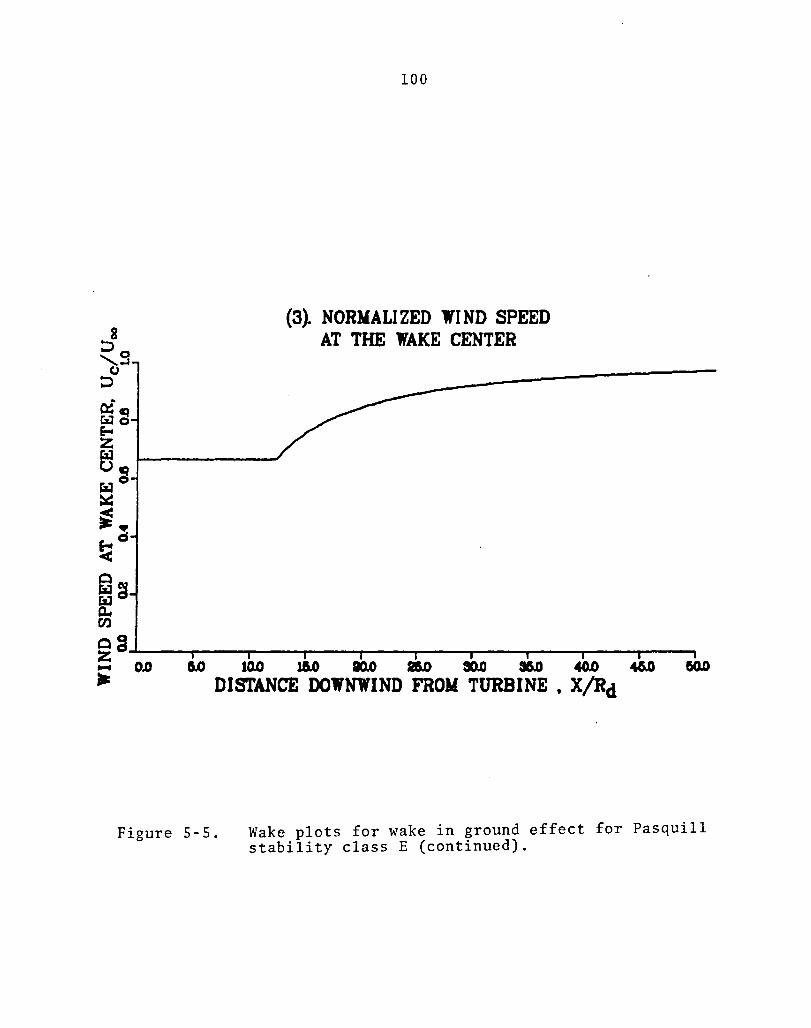
100

(3~ NORMALJ ZED WI ND SPEED AT THE WAKE CENTER

5.0 10.0 W) 10.0 ao 30.0 3&J) 40.0 DISTANCE DOWNWIND FROM TURBINE • X/Rd

Figure 5-5. Wake plots for wake in ground effect for Pasquill stability class E (continued).

~~ .......... c.. a!~

~ r:: ...

d a:: r:LI

~~ ~

0.0

101

(4). TURB I NE POWER FACTOR FOR AN UNBOUNDED WAKE

aD 10.0 16.0 ao.o ao 30.0 35.0 40.0 DISTANCE DOWNWIND FROM TURBINE • X/Rd

Figure 5-5. Wake plots for wake in ground effect for Pasquil1 stability class E (continued).

102

( 5). LATERAL WIND SPEED PROFILE

AT X/Rd = 5.00 Altitude of wind speed profile in rotor radii relative to the wake center

o ~~~--~~r-----------------------------

.. o trJ"! rx.l 0

0.. Cf.l

~~ Zo ...... ~

~

1.0

0.5

0.0

~----~----~------r-----~----~----~ 0.0 10 ao 3.0 4.0 5.0 6.0

LATERAL COORDINATE t Y/Rd

Figure 5-5. Wake plots for wake in ground effect for Pasquill stability class E (continued).

0 -I

8 ::>a;) "-.,.0 :>

~

~ UJ~ ~o 0.. U)

~~ Zo ..-~

~ 0

q

103

( 6). LATERAL WIND SPEED PROFILE

AT X/Rd = 10.00

2.0, 2.5

0.5

0.0

-1.0

o~----~----~----~----r-----r---~ 0.0 10 2.0 3.0 4.0 5.0 6.0

LATERAL COORDINATE t Y/Rd

Figure 5-5. Wake plots for wake in ground effect for Pasqui11 stability class E (continued).

N ~

9

8 :Jro --........0 ::>

.. ~ Cz:J~ ~o 0.. (f)

~~ Zd ...... ~

~ 0

104

( 7). LATERAL WIND SPEED PROFILE

AT X/Rd = 20.00

2.5

1.5

1.0

-1. 0, 0.5

0.0

-0.5

~ ~----~----~----~----~--~r---~

0.0 to 2.0 3.0 4.0 5.0 6.0

LATERAL COORDINATE I Y/Rd

Figure 5-5. Wake plots for wake in ground effect for Pasqui11 stability class E (continued).

105

( 8). LATERAL WIND SPEED PROFILE

AT X/Rd 35.00

_-2.5 ~~2.0

S~~~~~~1_.5 ____ ------

~1.0

.. o ~~ ~o 0.. Ul

O~ Zd toooo4

~

q

-1. 0 -0.5, 0.0, 0.5

o~----~----~----~----r-----r---~ 0.0 to 2.0 3.0 4.0 5.0 6.0

LATERAL COORDINATE t V/Rd

Figure 5-5. Wake plots for wake in ground effect for Pasquill stability class E (continued).

... o CiJ~ ~o a.. en o. zo ....... ~

106

( 9). LATERAL WIND SPEED PROFILE

AT X/Rd = 50.00

0. O~----~----~----r---~~--~----~

0.0 10 2.0 3.0 4.0 5.0 6.0

LATERAL COORDINATE I Y/Rd

Figure 5-5. Wake plots for wake in ground effect for Pasquill stability class E (continued).

107

(10). VERTICAL WIND SPEED PROFILES . AT WAKE CENTER

0.0

Figure 5-5.

Distance downwind of the turbine in rotor radii

50.,----..

35.----

20. ------..

10. ----

5.

Q2 Q4 Q6 O~ 10 WIND SPEED, U/Uoo

1.2

Wake plots for wake in ground effect for Pasquill stability class E (concluded).

108

(1). NORMALIZED WAK

~ Ambient turbulence represented by Pasquill stability class D

9

m = 1. 5

h = 1. 35 a

y = 0.15

~~----~--~~--~----~----~----~--~----~----~--~ . 0.0 &.0 10.0 I&.0 20.0 25.0 30.0 35.0

DISTANCE OOWNWIND FROM TURBINE

Figure 5-6. Wake plots for wake in ground effect for Pasquill s~ability class D.

-';:)0 I q~ ____ --. 8 .... .,-

';:) -"'--CD

dJd

t 8

';:).q -0

-u. t:d ~ o

~~ ff rtl

109

(2). NORMAUZED WIND SPEED DEFICIT AT THE WAKE CENTER

o~~ __ ~ ____ ~ __ ~ ____ ~ __ ~ ____ ~ __ ~ ____ ~ ____ --~ Z 0.0 -~ GoO 10.0 10.0 20.0 2&.0 30.0 36.0 40.0

DISTANCE DOWNWIND FROM TURBINE. X/Rd

Figure 5-6. Wake plots for wake in ground effect for Pasqui11 stability class D (continued).

110

(3). NORMAL! ZED WI ND SPEED AT THE WAKE CENTER

5.0 10.0 16.0 20.0 2&.0 30.0 35.0 40.0

DISTANCE DOWNWIND FROM TURBINE , X/Rd

Figure 5-6. Wake plots for wake in ground effect for Pasqui1l stability class D (continued).

Q -8~

0.. "-a.. -~ 0::0

0 E-e t)

t::. d

0:: rzJ

~~

~ 0.0

111

(4). TURB I NE POWER FACTOR FOR AN UNBOUNDED WAKE

5.0 10.0 16.0 20.0 26.0 30.0 36.0 40.0

DISTANCE DOWNWIND FROM TURBINE I X/Rd

Figure 5-6. Wake plots for wake in ground effect for Pasquill stability class D (continued).

q -8

::JIX) '-..,.0 ::J

.. Q wee ~o

0.. IJ)

Q~ Zd ...... ~

~ 0

q

112

( 5). LATERAL WIND SPEED PROFILE

AT X/Rd = 5.00 Altitude of wlnd speed profile in rotor radii relative to the wake center

2 . 0 , 2.5

1.5

1.0

0.5

0.0

o~-----r----~------r-----~----~----~ 0.0 to ao 3.0 4.0 5.0 6.0

LATERAL COORDINATE , Y/Rd

Figure 5~6. Wake plots for wake in ground effect for Pasquill stability class D (continued).

113

( 6). LATERAL WIND SPEED PROFILE

AT X/Rd = 10.00

~- 2.0, 2.5

1.5

9~~~~~~ __ -----------------------

~ o UJ~ r£lo 0.. U)

0..., Zd ...... ~

~

~-i:~ ---0.5, 0.5

0.0

~----.-----,-----~----~----~----~

0.0 LO 2.0 3.0 4.0 5.0 6.0

LATERAL COORDINATE I Y/Rd

Figure 5-6. Wake plots for wake in ground effect for Pasquill stability class D (continued).

114

( 7). LATERAL WIND SPEED PROFILE

AT X/Rd = 20.00

...--- 2.5

9 §~~~~~~i~Sli=i~S_O ____ ------_

t~ ~-1.0 :::> '--- 0 . 5

~ o W~ ~o

0... U)

o~ Zd -a=

'------1.0, -0.5,0.0

~~---~----~----~----~-----.----~ 0.0 10 2.0 3.0 4.0 5.0 6.0

LATERAL COORDINATE I V/Rd

Figure 5-6. Wake plots for wake in ground effect for Pasqui11 stability class D (continued).

115

( 8). LATERAL WIND SPEED PROFILE

AT X/Rd = 35.00

s ~~~S5""""----------------

.. ~ til~ ~o

~ Cf)

~~ Zd ...... ~

~ ~----.-----~----r---~~--~----~ 0.0 10 ao 3.0 4.0 5.0 6.0

LATERAL COORDINATE, Y/Rd

Figure 5-6. Wake plots for wake in ground effect for Pasquill stability class D (continued).

116

( 9). LATERAL WIND SPEED PROFILE

AT X/Rd = 50.00

9 .......... __ ------------------------------

· o CzJ~ tr:JO 0.. Cf.l

o~ Zo ~

~

~ ~----~----~----~----~--~------0.0 10 2.0 3.0 4.0 5.0 6.0

LATERAL COORDINATE I Y/Rd

Figure 5-6. Wake plots for wake in ground effect for Pasquill stability class D (continued).

117

(10). VERTICAL WIND SPEED PROFILES AT WAKE CENTER

~l

0.0

Distance downwind of the turbine in rotor radii

50.---

35.

20.--....

0.2 0.4 0.6 O.B 1.0

WIND SPEED, U/Uoo

1.2

Figure 5-6. Wake plots for wake in ground effect for Pasquill stabili ty class D (concluded).

Wake width

.118

Ambient turbulence represented by Pasquill stability class C

m = 1. 5

ha = 1.35

Y = 0.15

~~--------~~--~~~~-----r----~----'-----~----r----' .JJ 10.0 16.0 20.0 26.0 30JJ 36.0

DISfANCE DOWNWIND FROM TURBINE

Figure 5-7. Wake plots for wake in ground effect for Pasquill stability class C.

-";J0

19 oJ -""--~ d)O I 8

";J~ -0

e-. ...... U. fi:d ra:l Q

&i~ f;IJ C-OO

Q~ :z= -• • JJ

119

(2). NORMALIZED WIND SPEED. DEFI CIT AT THE WAKE CENTER

&.0 10.0 m.o 20.0 ZO so.o 36.0 40.0 .

DISTANCE DOWNWIND FROM T~BINE • X/Rd

Figure 5-7. Wake plots for wake in ground effect for Pasquill stability class C (continued).

8 ::>0 ,~

o ::>

g~ E-4 Z ~ C) ...--_----J

d ~ ~

~. ~

d

~~ ff Ul

120

(3). NORMALI ZED WI ND SPEED AT THE WAKE CENTER

t:l~ Z ~--~--------------~----~--~--------~----------- . .0 10.0 16.0 20.0 ZO 30.0 S6.O 40.0 ~ DISTANCE DOWNWIND FROM TURBINE , X/Rd

Figure 5-7. Wake plots for wake in ground effect for Pasqui11 stability class C (continued).

8~ 0..

" ~ o::~ 0 E-c U ~ ..

0 Q.:: r:zl

~~

~ • .0

121

(4), TURB I NE POWER FACTOR FOR AN UNBOUNDED WAKE

5.0 10.0 16.0 ao.o ZO 30.0 36.0 40.0

DISTANCE DOWNWIND FROM TURBINE. X/Rd

Figure 5-7. Wake plots for wake in ground effect for Pasquil1 stability class C (continued).

122

( 5). LATERAL WIND SPEED PROFILE

AT X/Rd = 5.00 Altitude of wind speed profile in rotor radii relative to the wake center

2.5

9~~~~~~---------------------------

.. ~ trJ~ ~o ~ rn ~. ZO ...... ~

0.5

'---- 0.0

"----- -1. 0

~~----~----~----~~----~----~----~ \ .0 10 2.0 3.0 4.0 5.0 6.0

LATERAL COORDINATE, Y/Rd

Figure 5-7. Wake plots for wake in ground effect for Pasquill stability class C (continued}.

123

( 6). LATERAL WIND SPEED PROFILE

AT X/Rd 10.00

91=~~~~~----------------

.. ~ ~~ ~o

~ rn ~~ Zd ...... a=

~ o

~

-1.0, -0.5, 0.0, 0.5

------~----~----~----r_----r_--~

\ .0 to 2.0 3.0 4.0 5.0 6.0

LATERAL COORDINATE I Y/Rd

Figure 5-7. Wake plots for wake in ground effect for Pasqui11 stabili ty class C (continuedl.

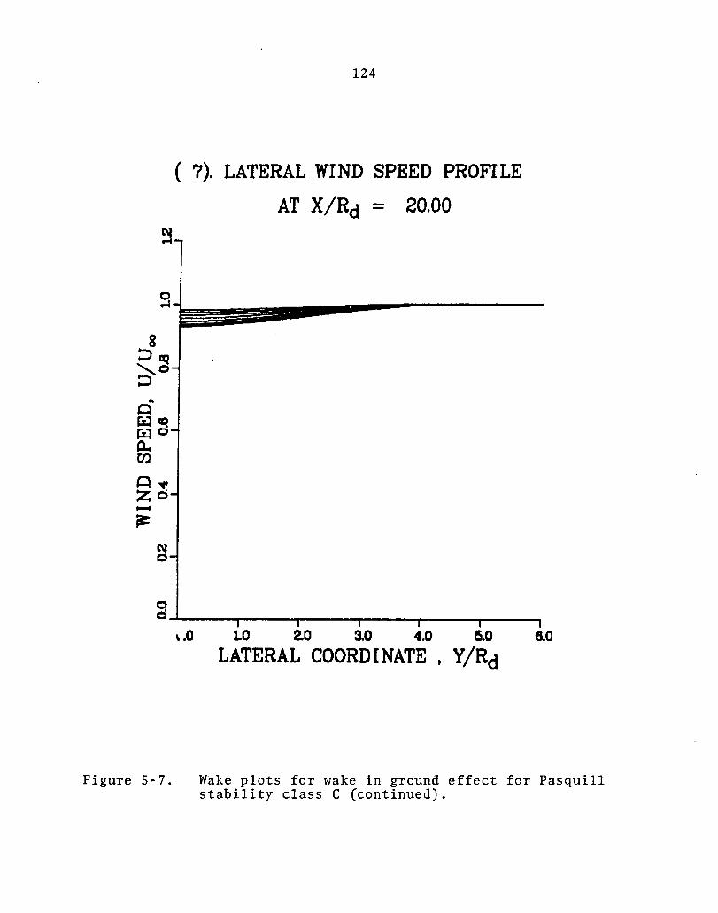
N ~.

8 ::>!q "",0 ::> 0" (IJ~ ~c a.. Cf.)

o. Zd ...... ~

124

( 7). LATERAL WIND SPEED PROFILE

AT X/Rd = 20.00

c. o~ ____ ~ ____ ~ __ ~ __________ ~ __ ~

\ .0 10 2.0 3.0 4.0 5.0 8.0

LATERAL COORDINATE t Y/Rd

Figure 5-7. W~ke plots for wake in ground effect for Pasquill stability class C (continued).

125

( 8). LATERAL WIND SPEED PROFILE

AT X/Rd = 35.00

9 ~ ________ ---------------------------------8

::>~ '0 ::> 0" t'iI~ ~o 0.. (J)

O~ Zd ...... ~

C. O~ ____ ~ ____ ~ ____ r-__ ~~ __ ~ ____ ~

\ .0 LO ao 3.0 4.0 5.0 6.0

LATERAL COORDINATE I Y/Rd

Figure 5-7. Wake plots for wake in ground effect for Pasquill stability class C (continued).

126

( 9). LATERAL WIND SPEED PROFILE

AT X/Rd = 50.00

9~---------------------------------

8 ~~ ,",,0 ::J

Q" (iJ~ ~o Q.. en Q. zo ..... ~

o O~----~----~----r---~~--~-----'

\ .0 LO 200 3.0 4.0 f;.O 6.0

LATERAL COORDINATE t Y/Rd

Figure 5-7. Wake plots .for wake in ground effect for Pasqui11 stability class C (continued).

q -

127

(10). VERTI CAL WI ND SPEED PROFI LES AT WAKE CENTER

Distance downwind of the turbine in rotor radii

35.------..

2 0 .=------'----..

o d~ ____ ~~~==~~~=-~----._--_.

I

1..0 0.2 0.4 0.6 0.8 1.0 1.2

V\TIND SPEED, U/Uoo

Figure 5-7. Wake plots for wake in ground effect for Pasquill stability class C (concluded).

128

m = 1. 5

8

7

6

stability

2[g~ __ ~:-No ambient turbulence

1

10 20 30 40 50

Distance downwind from turbine, X/Rd

Figure 5-8. Effect of ambient turbulence on wake radius.

r--. 0

;:::, 1.0 I

8 ;:::, '-' ........ r--. 0.8

u ;:::,

I

8 :::> '-' 0.6 .j-J

'M U

'M 0.4 4-i (l)

"Cl

"Cl (l) (l) 0.2 p. Ul

"Cl ~

'M 00 ~

129

m = 1. 5

No ambient turbulence

asqui11 stability class E

10 20 30

Distance downwind from turbine, X/Rd

Figure 5-9. Effect of ambient turbulence on wind speed deficit parameter.

.. I-< (1) 1.0

-l-J ~ (1)

u

(1) 0.8 ~ cO ~

(1)

'5 0.6

Figure 5-.10.

130

m = 1. 5

stability

No ambient turbulence

Distance downwind from the turbine,

Effect of ambient turbulence on wind speed at the wake center.

8 0.. .......... 0..

!-t 0 .j..J

u cd ~

!-t (J) :;: 0 p..

(J)

~ 'M ..0 !-t ::s

E-<

131

m = 1. 5

1.0

0.8 stability

0.6

----0.4 No ambient turbulence

0.2

OL-__ ~ __ ~L-__ ~ __ ~L-__ ~ __ ~ ____ ~ __ ~ ____ ~ __ ~

o 10 20 30 40

Distance downwind from the turbine, X/Rd

Figure 5-~~. Effect of ambient turbulence on turbine power factor.

50

8

7

6

5 ~--m=3

r---- 2

132

Pasqui11 stability class D

10 20 30 40

Distance downwind from the turbine, X/Rd 50

Figure 5-12. Effect of initial velocity ratio in the wake on wake radius.

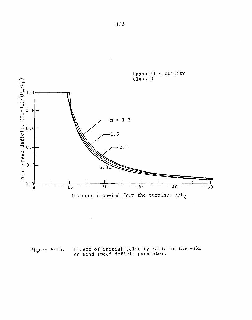
r--.. o

::::> I

8 ~ 1.0r---------~ '-' .......... r--..

U ::::>

I 0.8 8

::::> '-'

~ 0.6 .r-! u

.r-! lH (])

'"d O. '"d (]) (]) p..

Vl O. '"d ~

.r-!

~

133

Pasquil1 stability class D

O.O~--~----~--~----~----L---~~--~--~L----L--~ o 40

Distance downwind from the turbine, X/Rd

50

Figure 5-13. Effect of initial velocity ratio in the wake on wind speed deficit parameter.

I-< Q)

m = 1. 3

134

Pasqui1l stability class D

~ 0.8 Q) ~ ________ -J

U

Q)

~ cO 0.6 ~

Q)

...r::: +J

+J cO

"d Q)

0.4

~ 0.2 If)

1.5

2.0

3.0

Figure 5-14.

Distance downwind from the turbine,

Effect of initial velocity ratio in the wake on wind speed at the wake center.

1.0

8 p., .......... p.,

0.8 '"

I-< 0 .j...l u ro 0.6

lH

I-< (!)

::: 0 0.4 0..

(!)

I=: 'M ,.0 0.2 I-< ~

E-<

00

Figure 5-15.

135

Pasquill stability class D

10 20 30 40 Distance downwind from the turbine, X/Rd

Effect of initial velocity ratio in the wake on turbine power factor.

50

o

136

(10). VERTICAL WIND SPEED PROFILES AT WAKE CENTER

Pasqui11 class D m = 1. 5 h = 1 2 a .

y = 0.0

Distance downwind of the turbine in rotor radii

50.--","""

35. -----..

20.

o~ ______ ~ ____ ~ ______ ~ ____ ~~~~~ ____ ~ l.0 0.2 0.4 0.6 O.B 1.0 1.2

WIND SPEED, U/Uoo

Figure 5-16. Effect of the gound plane on the vertical wind speed profile for a rotor hub altitude of 1.2 rotor radii.

q

137

(10). VERTICAL WIND SPEED PROFILES AT WAKE CENTER

Distance downwind of the turbine in rotor radii

50.------.

35. ----,.

Pasquill stability class D m = 1. 5 h = 1. 35 ya= 0.0

O~----__ ~--__ ~ ______ ~ ____ ~ __ ~~-r ____ ~

l.0

Figure 5-17.

0.2 0.4 0.6 O.B 1.0 1.2

WIND SPEED, U/Uoo

Effect of the ground plane on the vertical wind speed profile for a rotor hub altitude of 1.35 rotor radii.

138

(10). VERTICAL WIND SPEED PROFILES AT WAKE CENTER

q

Distance downwind of the tur ine in rotor radii

50. -------,

35 . --------,

20. ----

10.--

5.

Pasqui11 stability class D

m = 1. 5

ha = 1.65 y = 0.0

o~ ____ ~ ______ ~ ________________ ~~ ____ ___

\.0 0.2 0.4 0.6 O.B 1.0

WIND SPEED, U/Uco

Figure 5-18. Effect of the ground plane on the vertical wind speed profile for a rotor hub altitude of 1.65 rotor radii.

12

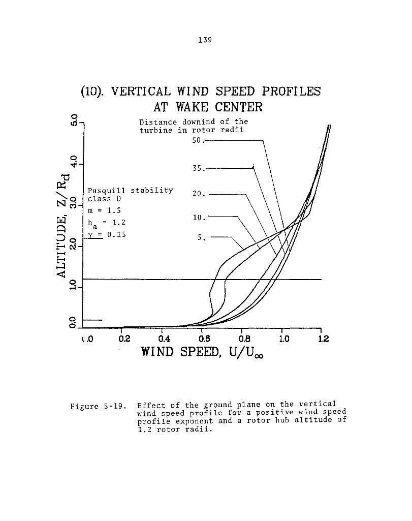
139

(10). VERTICAL WIND SPEED PROFILES AT WAKE CENTER

Distance downind of the turbine in rotor radii

Pasquill stability class D

l.0 0.2 0.4 0.6 O.B 1.0 1.2

Figure 5-19.

WIND SPEED, U/Uoo

Effect of the ground plane on the vertical wind speed profile for a positive wind speed profile exponent and a rotor hub altitude of 1. 2 rotor radii.

140

(10). VERTICAL WIND SPEED PROFILES AT WAKE CENTER

o ll'S

o ~

Distance downwind of the turbine in rotor radii

50 . --------,

Pasqui11 stability class D

35.------.

m = 1. 5

h = 1. 35 a y = 0.15

l.O 02 0.4 0.6 O.B

WIND SPEED, U/Uoo

1.0

Figure 5-20. Effect of the ground plane on the vertical wind speed profile for a positive wind speed profile exponent and a rotor hub altitude of 1.35 rotor radii.

1.2

o

141

(10). VERTICAL WIND SPEED PROFILES AT WAKE CENTER

Distance downwind of the turbine in rotor radii

5.----...

O~ ____ ~ __ ==~==~~~ __ ~ ____ -. ____ -,

LO 0.2 0.4 0.6 O.B 1.0 1.2

WIND SPEED, U/Uoo

Figure 5-21. Effect of the ground plane on the vertical wind speed profile for a positive wind speed profile exponent and a rotor hub altitude of 1.65 rotor radii.

'"d O!

142

(10). VERTICAL WIND SPEED PROFILES AT WAKE CENTER

Distance downwind of the turbine in rotor radii

50. -----.

35.--'"

""'0 Pasqui1l stability N ~ class D

m = 1. 5

h = 1.35

Y = 0.25

LO 0.2 0.4 0.6 O.B 1.0

WIND SPEED, U/Ueo

1.2

Figure 5-22. Effect of the ground plane on the vertical wind speed profile for a power law exponent for the free stream flow of 0.25.

143

6.0 CONCLUDING REMARKS

An analytic model for the calculation of the recovery of wakes of large wind turbines has been developed. The model is based upon the theory of co flowing turbulent jets as developed by G. N. Abramovich. The Abramovich model has been modified to relate turbine parameters to the wake parameters used by Abramovich, to add the effects of ambient turbulence to the model, and to calculate the turbine power factor, which is defined as the ratio of the power which a turbine in the wake of another turbine would generate the power which the turbine would generate if it were in the free stream air flow. The theory for the dis­persion of pollutants in a turbulent atmosphere as developed by F. Pasquill has been adapted to describe wake growth due to ambient turbulence, and the methods used by P. B. S. Lissaman have been used to combine the effects of wake growth as de­scribed by the Abramovich model with wake growth due to ambient turbulence.

This approach is currently considered to be the most ap­propriate approach for an analytical model of turbine wake re­covery. However, several intrinsic uncertainties about the model remain. A numberical approach (e.g., finite difference inte­gration of the three-dimensional Navier-Stokes equations) could be used. However, it is not considered appropriate, because comparable gross uncertainties would exist for this approach (e.g., magnitude of the turbulent fluctuations) and large costs would be incurred to generate solutions. Any further work on the model might best be directed toward expansions or refine­ments of factors within the existing formulation.

The literature has shown only very limited experimental evaluation of the model. Comparisons of computer results with experimental data are therefore, very much desired to establish the adequacy of the model and to resolve the questions involved. However, it is recognized that extensive data from full scale turbines are very difficult to obtain. An attempt to obtain such data is described in the companion report on the second (experimental) phase of the research program conducted by Lock­heed. Wind turbine model tests in wind tunnels may also be of use in validating some aspects of the model formulation. Al­though it would be almost impossible to duplicate the Reynolds number and geometry of an actual turbine in the wind tunnel, meaningful applicable results could be obtained. In another approach, the computer program may be used to determine the sensitivity of the final results to the factors in question.

1.

2.

3.

4.

5.

6.

7.

8.

9.

10.

11.

12.

13.

144

REFERENCES

Schlichting, H., Boundary Later Theory, Fourth Edition, McGraw-Hill, New York NY, 19 2.

Abramovich, G. N., The Theory of Turbulent Jets, MIT Press, Cambridge MA, 1963.

Templin, R. J., "An Estimate of the Interaction of Windmills in Wind Spread Arrays", Canada NRC, LTR-LA-171, Dec 1974.

Crafoord, C., "An Estimate of the Interaction of a Limited Array of Windmills", University of Stockholm Sweden, Nov. 1975.

Ljungstrom. 0., "Aerodynamic Interference Between Adjacent Wind Generators of the Conventional Horizontal Axis Type", Appendix 3-3, "Wind Power in Sweden", 1974.

Builtjes, P., Private communication with P. B. S. Lissaman, July 1977.

Lissaman, P. B. S., "Research Program on Energy Effectivess of Arrays of Wind Energy Collection Systems", Report AV SP 637, AeroVironment, Inc., Pasadena CA, 1976.

Anon., "Wind Flow Characteristics in the Wake of Large Wind Turbines", Report AV FR 8147, AeroVironment, Inc., Pasadena CA, Sept 1978.

Lissaman, P. B. S., "Energy Effectiveness of Arrays of Wind Turbines", Journal of Energy, v. 3, n. 6, Nov-Dec 1979.

Bird, R. B., W. E. Stewart, and E. L. Lightfoot, Transport Phenomena, John Wiley & Sons, Inc., New York NY, 1965.

Turner, D. B., "Workbook of Atmospheric Dispersion Estimates", Environmental Protection Agency, Office of Air Programs, Research Triangle Park NC, 1970.

Wilson, R. E., P. B. S. Lissaman, and S. N. Walker, "Aerodynamic Performance of Wind Turbines", Oregon State University, Corvallis OR, June 1976.

Slade, D. H. (editor), "Meteorology and Atomic Energy," U. S. Atomic Energy Commission TID-24190, 1968.

145

Appendix A

LIST OF SYMBOLS

This appendix contains a list of symbols us~d in the development of the analytic model. Where appropriate, variable names used in the FORTRAN computer program are also listed. The equation number, figure number, or table number following the definition is the equation, figure, or table where the parameter is defined or first used in the description of the analytic model.

A few parameters used in the deriviation have been omitted from this list. They are omitted if they are of minor importance and are used for only two or three successive equations in the derivation so that the location of their definition in the text is never in doubt.

Symbol

A

a

B

b

c

Computer Symbol

B

AH

AH

Definition

Cross-sectional area of the turbine disk. Equation (3-1).

Free stream cross-sectional area of the stream tube which. passses through the turbine disk. Equation (3-64).

Axial induction factor for the turbine. Equation (3-7).

Parameter used for the derivation of the turbine power factor. Equation (3-75).

Full width of the boundary layer in region I. Equation (3-36).

Partial widths of the boundary layer in region I. Figure 3-5.

Growth rate of the boundary layer in region I. Equation (3-59).

Hub altitude of the turbine in physical units. Table 3-2.

Hub altitude of the turbine nor­malized by the rotor radius. Table 3-2.

Symbol

h

I

i

J

K

m

n

P

Computer Symbol

AH

10

J

CPM

AN

PR

146

Definition

Height of the top of the wake above the ground. Equation (3-80).

Input parameter which specifies whether geometric input parameters are in physical units or normalized by the rotor radius. Table 3-2.

Index to define altitude of lateral wind speed profile. Equation (5-1).

Number of downwind locations at which wind speed profiles are to be calculated. Table 3-2.

Constant used in derivation of the turbine power factor. Equation (3-64).

Ratio of the free stream wind speed to the initial wind speed in the wake (after expansion by potential effects to wake radius, RO). Equation (3-9).

Mass flow rate of air passing through the turbine disk. Equation (3-1).

Ratio of the downwind extent of Region II to the downwind extent of Region I. Equation (3-47).

Power extracted from the air by the turbine. Equation (3-63).

Power extracted from the air by a turbine in the free stream. Equation (3-10).

Turbine power factor, which is the ratio of power extracted by a tur­bine in the wake of another turbine to the power which an identical turbine would extract in the free stream flow. Equation (3-63).

Symbol +

p

p

R

r

r . sJ

Computer Symbol

RRR

R2SAV

RO

147

Definition

Static pressure on the upwind side of th~ turbine. Equation (3-2).

Static pressure on the downwind side of the turbine. Equation (3-2).

Ambient static pressure. Equation (3-3).

Radial coordinate in physical units.

Radius of the turbine rotor disk. Figure 3-1.

Initial wake radius in physical units. Figure 3-1.

Radius of the potential core in Region I. Figure 3-1.

Wake radius in physical units. Figure 3-1.

Wake radius at the end of Region I in physical units. Figure 3-1.

Wake radius at the end of Region II in physical units. Figure 3-1.

Free stream radius of the stream tube which passes through the turbine disk. Figure 3-6.

Radial coordinate normalized by the turbine disk radius.

Wake radius at the jth downwind location at which wind speed profiles are to be plotted. Equation (3-84).

Initial wake radius normalized by the turbine disk radius. Equation (3-18).

Symbol

r ' 2

!:.r

T

u

Computer Symbol

R1

R2

R2P

R21

R22

RI

DR

148

Definition

Radius of the potential core in Region I normalized by the turbine disk radius. Equation (3-36).

Wake radius normalized by the turbine disk radius. Equation (3-24) .

Incremented value of R2 used in numerical inetgration for Region III. Discussion preceeding Equation (3-51).

Wake radius at the end of Region I normalized by the turbine disk radius. Equation (3-34).

Wake radius at the end of Region II normalized by the turbine disk radius. Equation (3-50).

Free stream radius (normalized by the turbine disk radius) of the stream tube which passes through the turbine disk. Equation (3-67).

Increment of r used for numerical integration in Region III. Equation (3-62).

Axial thrust on the turbine disk. Equation (3-1).

Local wind speed in the wake. Equation (3-32).

Wind speed at the center of the wake. Equation (3-81).

Wind speed of the air passing through the turbine disk. Equation (3-1).

Initial wind speed of the wake (after expansion to wake radius, RO)' Equation (3-1).

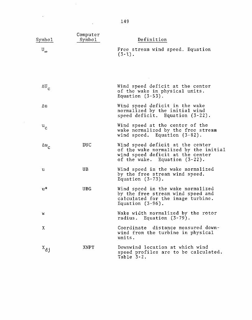
Symbol

flu

u

u*

w

x

Computer Symbol

DUC

UB

UBG

XNPT

149

Definition

Free stream wind speed. Equation (3-1) .

Wind speed deficit at the center of the wake in physical units. Equation (3-53).

Wind speed deficit in the wake normalized by the initial wind speed deficit. Equation (3-22).

Wind speed at the center of the wake normalized by the free stream wind speed. Equation (3-82).

Wind speed deficit at the center of the wake normalized by the initial wind speed deficit at the center of the wake. Equation (3-22).

Wind speed in the wake normalized by the free stream wind speed. Equation (3-73).

Wind speed in the wake normalized by the free stream wind speed and calculated for the image turbine. Equation (3-96).

Wake width normalized by the rotor radius. Equation (3-79).

Coordinate distance measured down­wind from the turbine in physical units.

Downwind location at which wind speed profiles are to be calculated. Table 3-2.

Symbol

XH

x

X'

Y

/::"y

z

Computer Symbol

x

XP

XH

XHM

XNPT

DYY

DYY

150

Definition

Downwind extent of Region I in physical units. Figure 3-1.

Downwind extent of Region II in physical units. Figure 3-1.

Coordinate distance measured downwind from the turbine, normalized by the turbine disk radius. Equation (3-20).

Incremented value of x used during the numerical integration in Region III. Equation (3-62).

Downwind extent of Region I normalized by the turbine disk radius. Equation (3-39).

Downwind extent of Region I from Abramovich solution normalized by the turbine disk radius. Equation (3-47).

Downwind location at which wind speed profiles are to be calculated, normalized by the rotor radius. Equation (3-83).

Lateral coordinate measured from the vertical center of the wake in physical units.

Increment in the lateral coordinate used in generating the wake profile. in physical units. Table 3-2.

Increment in the lateral coordinate used in generating the wake profile, normalized by the turbine rotor radius. Table 3-2.

Vertical coordinate measured positive upward from the ground in physical units.

Symbol

z

~Z

~z

a

y

~KE

n

p

cr

Computer Symbol

Z

ZVAL

ZO

DZZ

DZZ

ALPHA

N

ST

151

Definition

Vertical coordinated normalized by the turbine rotor radius.

Altitude relative to the turbine hub, normalized by the rotor radius. Equation (3-85).

Altitude of the lowest wind speed profile in physical units. Table 3-2.

Altitude increment between successive wind speed profiles in physical units. Table 3-2.

Altitude increment between successive wind speed profiles normalized by the rotor radius. Table 3-2.

Wake growth rate due to ambient turbulence. Equation (3-28).

Exponent for the power law wind speed profile. Table 3-2.

Change in kinetic energy of the air passing through the turbine. Equation (3-10).

Non-dimentional radial parameter used in Region I. Equation (3-33).

Mass density of ambient air. Equation 3-1.

Pollution dispersion coefficient from plume theory. Equation (3-19).

Standard deviation of wind direction in the ambient air. Table 3-2.

15Z

Appendix B

PROGRAM LISTING

The following pages contain a listing of the FORTRAN computer program used to calculate turbine wake progerties and to generate plots of wake properties. Comments in the program listing describe the sequence of calculations. Equation numbers given in the listing give the equation numbers in the text of this report.

The main program is listed first with suboutines following. Subroutine R3 calculates the wind speed deficit parameter, ~u ; the wake growth rate due to mechanical turbulence, CdrZ/dx) ;c and the turbine power factor, P, in Region III. Subroutinem

CALCU is used to calculate the wind speed profiles. The remaining suboutines are plotting suboutines used to generate appropriate plots. Subroutine XVSRZ is used to plot wake boundary parameters as a function of the downwind coordinate, x. Subroutine XVSDUC is used to plot the wind speed deficit parameter, ~u , as a function of x. Subroutine XVSUB is used to plot the wind speed at the wake center as a function of x. Subroutine XVSPR is used to plot the turbine power factor, P, as a function of x. Subroutine YVSUBR is used to generate the plots for the lateral wind speed profiles. Subroutine UVSZ is used to generate the plots for the vertical wind speed profiles.

c c c c. c c C C C C

TITLE t YAICE

AUTHORS I DR. W. ElEJlLE A. C. SCOPPA

153

LOCKHEED "ISSILES AND SPACE CO.

C ••• THIS PROCRAft CALCULATES "AKE'PAR~TERS FOR THE RECOVERV C ••• OF UAKES OF·lARCE WIND TURlIHES. THE PROCRA" PLOTS ~AKE C ••• RADIUS. UAKE WIDTH. WAKE ALTITUDE. THE WIND SPEED DEFICIT C • • • AT THE CENTER OF THE ~AKE. THE WIHD SPEED AT THE CENTER C ••• OF THE.UAKE. AND THE TURIINE PO~ER FACTOR AS FU"CTIONS OF C • THE DISTANCE DOWNWIND OF THE TURIINE. IN ADDITION. WIND SPEED C • PROFILES OF THE WIND SPEED AS A FUNCTION OF THE LATERAL C. • COORDINATE ARE PLOTTED FOR EICHT ALTITUDES FOR EACH DOWNWIND C •• LOCATION SELECTED IV THE USER. A VERTICAL WIND SPEED PROFILE C • • • IS GENERATED FOR EACH DOUN~IND LOCATION SELECTED FOR PLOTS OF C • OF LATERAL WIND SPEED PROFILES. C C C C C ••• sT C C C C C C C C C C C C C C C C C C C

• CP"

• AH

C ••• VHI C C C C C ••• UEXP C C C C • RRR

- A1f'OsPHfJUC TURIULENCE PARAI'IATER. IF INPUT AS A POSITIVE N~BER, IT IS THE STANDARD DEVIATION OF THE ~I"DDIRECTION. IF INPUT AS A NEGATIVE HU~IER. IT IS THE PAsOUILL sTAIILITY CLASS AS FOLLO~St -1 FOR PASOUILL STAIILITY CLASS A -2 FOR PASOUILL STABILITY CLASS I -3 FOR PASOUILL STAll LIT'll CLASS C -~ FOR PASOUILL STAIILITY CLASS D -S FOR PASOUILL STAIILITY CLASS E -6 FOR PASOUILL STAIILITY CLASS F IF S1 IS IHPUT AS e •• AN ,,"IIEHT TURBULENCE OF ZERO IS USED. AND THE RESULTING PROFILES ARE THE ABRA~ICH SOLUTIONS.

- RATIO OF FREE STREAM WIND SPEED TO INITIAL ~IND SPEED IN THE ~AICE

- HUI HEIOHT I~ ROTOR RADII OR IN PHYSICAL UNITS AS SPECIFIED IV 10

- ~BIENT WIND SPEED AT HUB ALTITUDE. THIS ~AY IE ClUEN IN PHYSICAL UNITS IF OUTPUT IS DESIRED IN PHYSICAL UNITS • Nt IHPUT VALUE OF 1. I WILL CIVE OUTPUT NO~LIZED I'll THE FREE STREAM WIND STREAM.

- COEFFICIENT OF THE WIND SPEED POWER LAW OF THE FORft "U-V.'(Z/ZI)'IWEXP"

- JlOTOR RADIUS. THIS "A'll IE GlUEN IN PHYSICAL UNITS. AN INPUT VALUE OF 1.1 WILL GlUE ALL OUTPUT

C C C C C C C • J C C C ••• 10 C C C C C ••• NP C C C C C C ••• XNPT C C C C ••• ze C C

C ••• DZZ C C C C C C

• • • DYY

154

OF lI"ITS OF' LENGTH Itt ROTOR RADII. M INPUT VALUE OF • 5 ~ILL GIVE Al.l.OUTPUT OF' UNITS OF LEHGTH IN ROTOR DIAMETERS. AN IHPUT VALUE CREATER THAN 2.' YIl.L aIVE ALl. OUTPUT OF UHITS OF LENQTH IN THE PHVSICAl. UNITS USED FOR THE ROTOR RADIUS.

- HUMIER OF DO~N UIND LOCATIONS AT UHICH ~IND SPEED PROFIl.ES ARE TO IE CAl.CULATED

- INPUT OPTION FOR PAR~ETERS ~ITH PHYSICAl. DIMENSIONS (AH.XNPT.Ze.DZZ.DVY) 1 FOR INPUT IN ROTOR RADII 2 FOR INPUT IN PHYSICAL UNITS

- SPECIFIES HOU VEl.OCITY IS TO BE NORMALIZED FOR PLOTS OF ~IND SPEED PROFIl.ES IN l.ATERAl. DIRECTION. NP • e NORMAl.IZES UIND SPEED BV THE FREE STREA" UIND SPEED AT THAT ALTITUDE. NP • 1 HORMAl.IZES UIND SPEED BY THE FREE STREAft UIND SPEED AT THE HUB ALTITUDE.

- DOUHUIND l.OCATIONS AT UHICH UIND SPEED PROFIl.ES ARE TO BE CAl.CULATED (ROTOR RADII OR PHYSICAL UNITS AS SPECIFIED BY 10

- "INI"U~ ALTITUDE AT UHICH YIND SPEED PROFILES ARE TO BE - CAl.CUl.ATED (ROTOR RADII OR PHVSICAL UNITS AS SPECIFIED

IV 10)

- INCREMENT IN Al.TITUDES AT YHICH ~IND SPEED PROFILES ARE TO BE CAl.CUl.ATED (ROTOR RADII OR PHYSICAL UNITS AS SPECIFIED IV 10)

- INCREMENT IN Y BV UHICH CAl.CUl.ATIONS ARE TO BE "ADE IN GENERATING THE UIND SPEED PROFILES (ROTOR RADII OR PHYSICAL UNITS AS SPECIFIED BV 10)

C C C C

CONTROl. INPUT I

C C C C C C C C C C C C C C C C

RECORD 1 - (S0Fle.~) [S INPUT VARIABLES) ST.CPM.AH.VHe,UEXP,RRR

RECORD 2 - (5912) [3 VARIABl.ES] J,IO,HP

RECORD 3 - (SeFle.~) [J VARIABLES] )eMPT

RECORD ~ - (Sefle.4) [3 VARIABLES] Ze.DZZ.DVV

OUTPUT FILES I ONE DATA SET PER PLOT, KAMING COHVENTION ·SUBNAME.DAT"

155

c C "ISCELLAHEOUS I C THE PLOTTING PACKAGE 'DISSPLA" ~ST IE LINKED YITH C "W~E' .EFORE EXECUTION. THIS PROGR~ C CAH .E RUN 'AS IS" USING A PDP-II C~ILER AND A C TEKTROHIX 4114 EXTENDED GRAPHICS TERftINAL. OTHERWISE C EXTENSIVE ftODIFICATIONS YILL IE HECESSARV. C

COftftOH /SU.CO"/ CP".AH.RI.R2.DUC.U'.UBC.DRDX.PR.

C

C

C

C

C

C

C

• XH.R22.R21.XH

C~ON /PSCALE/ RRR.VHt

CO~N /CRPA/ICRT,IPAPER

DOUBLE PRECISION IHFILE.UFILE

REAL XNPT(at).R2SAU(2t)

DATA ICRT/l/,FLAC/-gg./,[/2.7182818/

DATA IUBAR/'U.AR'/

C DETERftINE DATA SET SPECS FOR CONTROL INPUT C

WRITE(S,S) S FOR"AT(' EHTER LOGICAL UNIT AND FILE HA"E WHERE'.

I ' CONTROL INPUT RESIDES .') C

READ(S.7)IHU.IHFILE 7 fOR"AT(I2.AS) C C • OPEN DATA SET CONTAININC CONTROL INPUT C

OPEN (UNIT-IHU,fILE-IHFILE,ACCESS-'SEQIN'.DISPOSE-'SAUE'. I DEUICE-'DSK')

C C • READ IN COHTROL DATA C

READ(IHU,l.) ST.CPft.AH.UHI.UEXP.RRR 18 FOR"AT(SeFlt.4) C

READ(IHU.29) J.IO.NP 28 fORftAT(5'I2) C

C

C

READ(IHU.1I) (XHPTCI),I-l,J)

READ(IHU,18) Zt.DZZ.DVV

C • • • CALCULATE PARA"ETERS IN ROTOR RADII iF THEV HAVE C • • • IEEN INPUT IN PHYSICAL UNITS C

If(.NOT.(IO .EG. a» GO TO 2S C EOUATIOH C3-12)

c C

C

c

z,-ze,RRR

DZZ-DZz/RR"

DVV-DYV'RRR DO as I-l.J

XNPT(I)-XNPT(I),RRR 26 CONTINUE 25 CONTINUE C C • C • • • CALCULATE CONSTANTS C • C C • • .SET VALUE FOR ALPHA C 3. CONTINUE C

IF< ST • CT. ,.) t ALPHA-l.g7'1 •• 31'Ett(.eStST)

IF(ABS(ST) .LT. I.E-I') t ALPHA-'.

IF(AIS(ST+l.) .LT. I.E-I.) t ALPHA-l.97t.212

IF(ABSCST+2.) .LT. I.E-I.) • ALPHA-l.97t.1S6

IFCABSCST+3.1 .LT. I.E-I" • ALPHA-l.g7t.l'"

IF(ABS(ST+4.' .LT. I.E-I" , ALPHA-l.g7t.16g

IF(ABSCST+S.) .LT. 1.E-lll , ALPHA-l.97t.es.

IF(ABSCST+6.) .LT. I.E-lt) , ALPHA-l.97t.e34

3S CONTINUE C C • SET VALUE FOR RADIUS CHANGE C

DR-.ea C

156

EOUATIOft (3-13)

EQUATIOtt (3-14)

EQUATIOH (3-15)

EQUATIOH (3-83)

EQUATION (3-28)

C CALCULATE INITIAL UAKE RADIUS IN ROTOR RADII C C EQUATION (3-18)

C C CALCULATE ~AKE RADIUS AT END OF REGION I C C EQUATION (3-34'

C C CALCULATE DOYNUIKD EXTENT OF REGION I IY AIRA"OUICH 'c C EQUATION (3-35)

157

XHft-R"Cl.+CP")/ t C.21'(CPft-l)'SORTC.214+.144'CPft))

C C • • • CALCULATE DO~HUIND EXTENT OF RECION I IN PRESENCE OF C • AftBIENT TURBULENCE C

XH-'.S'R21/SQRT(C'.S'R21/XH~)*.a+ALPHA*'2) C C CALCULATE UAKE PARAftETER AT THE END OF RECION II C C EQUATION C3-41)

AH-SQRTC.214+.144'CPft)* I Cl.-SQRTC.134+.124*CPft»)/ • (Cl.-SQRTC.214+.144'CP"))' I SQRTC.134+.124'CP"))

C EQUATION (3-46)

R22-R0+AN*(R21-R8) X-XN R2-R22 CALL R3

48 CONTINUE C C •• SAVE VALUES OF UAKE RADIUS AT INPUT VALUES OF C •• XNPTCI) FOR THE XNPTCI) UHICH LIES IN REGIONS I OR III C

DO 5S I-l,J IF(.NOT.(XHPT(I) .LE. XN)) GO TO S4

C EQUATION C3-84) R2SAVCI)-R8+CR22-Re)tXNPTCI)/XN

54 CONTINUE 5S CONTINUE C C C •• CREATE FIRST SET OF PLOT FILES FOR UAKE RADIUS, C •• UAKE ~IDTH, UA(E ALTITUDE, UIND SPEED DEFICIT AT THE CENTER C • OF THE ~~E, UIND SPEED AT THE CENTER OF THE UAKE, AND C •• THE TURBINE PO~ER FACTOR AS A FUNCTION OF THE DISTANCE C •• DOUN UIND OF THE TURBINE C C

C C

OPENtUNIT-18,DEVICE-'DSK',ACCESS-'SEQOUT', I ~ODE-'ASCII',DISPOSE-'SAVE',FILE-'XVSR2.DAT')

OPENIUNIT-ll,DEVICE-'DSK',ACCESS-'SEQOUT', • ~ODE-'ASCII',DISPOSE-'SAVE',FILE-'XVSDUC.DAT')

OPENCUHIT-12,DEVICE-'DSK',ACCESS-'SEOOUT', • ftODE-'ASCII',DISPOSE-'SAVE',FILE-'XVSU •• DAT')

OPENCUNIT-13,DEVICE-'DSK',ACCESS-'SEOOUT', I ftODE-'ASCII',DISPOSE-'SAVE'.FILE-'XVSUIC.DAT')

OPENCUHIT-14,DEUICE-'DSK',ACCESS-'SEQOUT', • ftODE-'ASCII'.DISPOSE-'SAVE'.FILE-'XVSPR.DAT')

FIRSTX-••

c c c c c c C

C

C

FIRSTV-R, FVa-R,+AH FYl-R •• a

URITEC1 •• l.) FIRSTX,FIRSTV,FV8,FVl

FIRSTY-l.

URITECll.1') FIRSTX.FIRSTV

FIRSTY-l • .ICPI1

URITE(12.1') FIRSTX,FIRSTV

F1RSTV-l • .ICPI1

URITEe13.1') FIRSTX.FIRSTV

XOLD-X RaOLD-R2

158

C • • • SEARCH THROUGH X. TERI1IHATE YHEN R2 IS GREATER THAH 8 , C • OR )( IS GREATER THAN sa .

C 6. CONTINUE

IFC.NOT.eRa .LE. 8 •• AND. X .LE. 52.» GO TO 78 IFe.NOT.ex .EQ. '.»CO TO 61

R2-Re DUC-l. UB-1..ICPrt UBC-l./CP"

61 CONTINUE IF(.HOT.CX .EO. XH» GO TO 62

Ra-R22 DUC-l. UB-I • .ICPM UBC-l./CPPI

6a CONTINUE RADDAH-R2+AH RPlUL2-Ra1:a. YRITE(18.1e) X.R2.RADDAH.~La URITE(ll.le) X,DUC URITEe12.1') X,U. URITEe13.1') X.U.C IFe.NOT.ex .HE ••• » co TO 63

URITEe14.1') X,PR 63 COHTIHUE

DO 6; I-l.J IFe.HOT.eXHPTCI) .CT. XH» CO TO 68

IFe.HOT.ex .CT. XNPTCI) • .AHD. • XOLD .LT. XHPTeI») CO TO 66

R2H£U-(eR2-R20LD)~()(-XOLD».CXHPT(I)-)(OLD)+R20LD R2SAUU )-R2HEY

159

66 CONTINUE IFC.HOT.C~ .EQ. XHPTCI») GO TO 67

R2SAVU )-R2 67 COHT I I'fUE 68 CONT I I'fUE 69 CONTINUE

)(OLD-X A20LD-A2 A2P-R2+DR CALL AJ DRDXE-SORTCCCDADX+DRDxp)~a.)**2+ALPHA'*2) XP-X+DR/DRDXE R2-R2P )(-XP DRD~-DRDXP CO TO 68

78 CONTINUE C C • CLOSE FILES C

C

CLOSECUNIT-l' ) CLOSE(UI'fIT-U) CLOSE(UNIT-12) CLOSE(UNIT-1J) CLOSE(UNIT-14)

C • 1l'fITIALIZE PLOTTER FOR DISSPLA, 1200 lAUD RATE. E)(TEI'fDED C GRAPHICS TERMINAL C

CALL TKTRN(12e,1) C C PRODUCE PLOTS C

CALL )(USR2 CALL XUSDUC CALL )(USUB

C CALL XUSUBG CALL XVSPR

c c • c . • • GENERATE YIND SPEED PROFILE PLOTS AS A FUNCTION OF THE C • • • LATERAL COORDINATE. FOR EIGHT ALTITUDES FOR EACH C • • • DOYNYII'fD LOCATION SELECTED BY THE USER. ALSO, A C • • • VERTICAL YIND SPEED PROFILE IS CEI'fERATED FOR EACH C • • • DOYNYIND LOCATIOtt SELECTED. C • C

IUtiITZ-J+14+1 OPENCUHIT-IUNITZ,FILE-'UVSZ',DEUICE-'DSK',"ODE-'ASCII'.

S DISPOSE-'SAUE'.ACCESS-'SEOOUT') DO 168 I-l,J

YRITECIUHITZ.ll) FLAC IUNIT-I+1" EHCODEC8.7S,UFILE) IUJAR,IUHIT FORI'IATtA".I2)

C C C

C

C

C

STEP THROUGH EICHT ALTITUDES

DO 14' JJ-l.8 YRITECIUHIT.l') FLAQ Y·t. UIAR-e.

160

COHTItruE IFC.HOT.CAIS(l.-U'AR) .CT ••••• '1)) GO TO 13.

WAL-Y EQUATION (3-8;'

ZUAL-AH-Z CAll CAlCUCYVAl.ZVAL,XNPT,R2SAU,I,U'ARA) WAL-Y

EQUATION (3-V;' ZUAl-AH+Z CALL CAtcUeYVAL,ZUAt,XNPT,R2SAU,I.UIAR')

EQUATION (3-518, IFeNP .EQ • .,

• UIAR-t.Me*CU'ARA+UIARI-l. ) C EQUATIONS (3-518) AND (3-5151)

IFeNP .EQ. II • UIAR-VH'''UJARA+U.ARI-l. ,. • (Z~AH"'UEXP

~RITE(IUHIT.lt' Y.U.AR Y-Y+DVV CO TO 5It

13. CONTINUE '1-6. UBAR-1. URIT[CIUNIT,lt'Y.U.AR Z-Z+DZZ

14. COHTINUE C C • CALCULATE VERTICAL ~IND SPEED PROFILES C

WAL-t. Z-'. 145 CONTINUE IFC.HOT.CZ .LE. 5.)'00 TO 158

C EQUATION C3-85)

C

C

ZUAL-AH-Z CALL CALCU(YUAL.ZVAt,XHPT.R2SAU.I,U.ARA) ZVAL-AH+Z

EQUATION (3-SlS) CALL CALCUCYUAt.ZUAL,XHPT,R2SAU.I,U.ARI)

EOUATIONS C3-SlI) AND (3-5151) U'~-UHt'(U'ARA+UIAR'-l.)'(Z/AH)"UEXP URITE(IUHITZ,I.' UIAR.Z Z-Z+DYV QO TO 141

161

15e ~TIHUE C

CLoS£eUNIT-IUHIT) C C FOR EACH OF THE 'XHPT', PLOT LATERAL YIND SPEED PROFILES C

CALL VVSUIReIUNIT.UFILE.XHPT,I) C 16t COHTIHUE C

CLOSEeUHIT-IUNITZ) C C PLOT VERTICAL WIND SPEED PROFILES C

CALL uuszeIUHITZ,'UVSZ'.AH,J) C C TEAnIMATE PLOTTINC SESSION, END PROGR~ C

CALL DOH£PL C

END

162

SUBROUTINE R3 c C • THIS SUIROUTINE CALCULATES WAKE GROWTH RATE, WIND SPEED AT THE CENTER OF C • THE WAKE, AND POYER RATIO IN REOION III OF THE WAKE. C

C C

CO""ON ,SUBCO", CPft.AH,R',R2,DUC,UJ,UJG,DRDX,PR, I XN,R22,R21,)(H

C • CALCULATE WIND SPEED DEFICIT AT THE CEHTER OF THE WAKE C C [QUATIOh (3-53'

DUC-3.73.1-.2S8SCP"'(1.-CPft'-SQRT«.2S8.CPft'(1.-CPftJ)I.2 I +.S3i'(R2.R2,cl.-CPM)'R •• '2J)

C C • • • CALCULATE WAKE GROWTH RATE DUE TO ftECHAHICAL TURBULENCE C C [QUATIOH (3-6"

C C CALCULATE HON-DI"ENSIONAL WIND SPEED AT THE WAKE CEMTER C EQUATIOH (3-94)

C

C

UI-l.-DUC.(t.-l.'CP"'

UBC-UB

C • IS THE CENTER OF THE WAKE IN GROUND EFFECT ? C

IF(.NOT.CR2 .CT. 2.SAH) CO TO 1. UF·l.-DUC'(1.-1.'CP")'Ct.-C2.'AH/R2"'I.S)"2 U.C·UUUF

19 CONTINUE C C CALCULATE THE RATIO OF POVER GENERATED IN A CEOftETRICALLV C. • IDENTICAL TURBINE CENTERED IN THE WAKE OF THE UPWIND TURlIHE C • • • TO THE POUER THAT TURBIhE WOULD GENERATE IF IT UERE IN THE C • • • STREA" UIND C EQUATION (3-75)

C [QUATIOH (3-71) Fl-(I.-3".+3.'.SS2-1.11'*3)/2. F2-(i.II-12,'.'S2+6.'."l',3.S F3-(-3.SB+18.*.'I2-1S.II"3"S, F4-(-12.*8'I2+29,'1'13"6.S F5-C3'1"2-15,""3)/8. F6-i.IIU3/9.5 F7-BU3,C-I1. , RI·SQRTCCCPM+l."(2.ICPft) RIR·RI/R2 PR·2.'CF1+F2'RIRI'I.5+F3'RIR'I3

• +F4.RIRI'4.S+FS.RIRI.i+FSIRIR •• 7.5+F7,RIRI*V) RETURN END

C C C C • C • C

c c C C C

163

SUtROUTINE CALCUCY.Z.XNPT~.RaSVD~.I.U.AR'

• THIS SU.ROUTINE CALCULATES ~IND SPEED IN THE YA(E FOR • CIVEH VALUES OF THE LATERAL AHD VERTICAL COORDINATE

DISTANCES • THE FOR" OF THE YIHD SPEED PROFILE OF • • REGION I • REGION II • OR RECION III AS APPROPRIATE

CO""ON /SU.CO~/ CP~.AH.R'.R2.DUC.U •• UJG.DRD~.PR. I )cN.R22.A81.)cH

REAL )cHPTD~C2el.N.R2SVD~e2G'

R-SORTCVtt2+Z.t21

DETER~INE IF )cNPT IS IH RECION I

IFC.NOT.C)cHPTD~(II .LT. )CH') GO TO 1&8 RI-R&-Re.)CNPTD"CI)/)(H R2-R2SUDrH I' H- CR-R2 )/CRI-R2) IFeH .LT. e.) UIAR-I. IFCH .CT. I.) U8AA-I./C~ IFce •• LT. H .AND. N .LT. 1.)

• UJAR·I./CP~+Cl.-1./CP") • '(1.-H"1.S)"2

I EQUATION (3-86)

EQUATION (3-87)

EQUATION (3-33) EQUATION C3-89) EQUATION' (3-88)

EQUATIOH (3-9') lee CONTINUE C C • DETER"INE IF )cttPT IS IH RECION III C

IF(.NOT.C)(HPTD"CII .QT. )CN') CO TO lie R2-R2SUD"CI) CALL R3 IFCA .GT. R21 UJAR-I IFCR .LE. R2) UBAR-l.-DUC.C1.-1./CP"'

I lCl.-CR/R2)U1.Sla.a

EQUATION (3-91)

EQUATION (3-93) lie CONTI~UE C C • DETERMINE IF XNPT IS IN REGION II C

IF(.NOT.(XH .LT. XNPTDMCII .AND. )cNPTDMCI) .LT. )cH» GO TO la. Rl-e. R2-R2SVD'H I ) N-CR-R2)/(RI-R2) EOUATIOH (3-33) IFCN .LT. e.) UJAR1-1. EOUATION (3-89) IFCH .QT. I.) U.AR1-1./CP~ EQUATION C3-88) IFC ••• LT. H .AHD. H .LT. I.)

• U.ARI-I./CP"+(I.-1./CP") I ICI.-Ntll.Sllt2 EOUATION (3-9')

Due-I. IFCR .CT. R2J U.AR2-1. EQUATION (3-94) IFIR .LE. R2)

I U.AR2-1.-DUCICI.-I./CPft) * 1(1.-(R/R2'tll.S)lt2 EQUATIOH (3-93) U.AR-CC)cHPT~CI)-)cH)/()(N-~H»IUJ~R2

I +(()(N-XttPTDftU»/()CN-)cH"IU.~R1 ! EQUATION (3-95) C CALL IOUAIT

CALL HDCOPV C C TER~IHATE PLOT C

CALL ENOPL") c C RETURM TO MAINLINE C

RETURH END

C

C

e C

C C . . . C

C

SUIROUTINE XVSR2

CO~ON ~PSCALE~RRR.VHt

REAL YVAL(3)

HLINES-J

SET nAXI~" VALUES FOR X AttD Y AXIS

)(!'IAX-S0. VMAX-S.

IFe.HOT.CRRR .GT. a.)) GO TO 5 Xl'!AX-S0.1RRR VMAX-8.1RRR

5 CONTINUE C

C

)(SCALE-XMA)(~se. VSCALE -VMA)(/8.

C • RE-INITIALIZE PLOTTER C

C

CALL BGNPLC 1) CALL PHVSORCl •• 1.) CALL PAGEC1~.,11.)

C PLOT AxIS C

CALL HEICHTce.Z) CALL COI'IPLX CALL MXIALFC'STAND'.'.') CALL MX2ALFC'L/CSTD',"') CALL MXJALFC'IHSTR','.') CALL TITLEl' ',I,

164

1 'DISTANCE DOUNUIHD FROM TURBINE , X~R'LH1.ID"',

C C

• lee,'UAKE BOUNDARY PARAMETER", • le0,le.,8.)

CALL GRAPH(e.,XI'IA)(~18 •• e.,YMAX~8.) CALL HEADIN('(111). NORMALIZED YAKE JOUNDARIES ",18e,1.,l'

C •• DRAY ONE LINE EACH FOR ~AKE RADIUS, YAKE C • RADIUS PLUS ALTITUDE, AND TYO TIMES YAKE RADIUS C • C C • • • OPEN DATA SET FOR EACH LINE C

DO ~e I-l.NLINES OPEN (UHIT-l',FILE-'XUSR2.DAT'.ACCESS-'SEQIN')

C C • • • READ FIRST CARD C

18 F~AT(SeFl'.4)

C

XPOS-(l'.~X~X'*XUAL*XSCALE YPOS-(I.~Y~)*YUAL(I)*YSCALE CALL STRTPT(XPOS.YPOS)

C • PLOT ENTIRE DATA SET C 28 CONTINUE

XPOS-(l'.~X~X)*xUAL*XSCALE YPOS-(8.~Y"AX)*YUAL(I'*VSCALE CALL COHHPT(XPOS.VPOS)

165

READ(18.18.END-3') XUAL.(VUAL(J).J-l.NLINES) GO TO 28

38 CONTINUE C C • CLOSE DATA SET C

CLOSECUNIT-18' C 48 CONTINUE C C • • • ftAKE A HARD COPY AND ERASE SCREEN C C CALL IOUAIT

CALL HDCOPY C C TERftINATE PLOT C

CALL ENDPL(l) C C RETURN TO MAIN ROUTINE C

RETURN END

c c

SUlROUTINE XUSDUC

CO""ON /PSCALE/RRR.UH.

166

C SET "AXII'IUft UALUES FOR X AND Y AXIS C

C IFC.HOT.CRRR .GT. 2.') 00 TO 5

)mAX-5' •• RRR 5 COHTIHUE C

IFC.NOT.CUHe .GT. 1." GO TO 6 YPlAX-l •• UH.

6 CONTINUE C

C

XSCALE-X,.,AX/S0. YSCALE-YI'IAX/l.

C. • OPEN DATA SET C

OPEN CUNIT-l1,FILE-·XUSDUC.DAT'.ACCESS-'SEQIH" C C RE-INITIALIZE PLOTTER C

C

CALL IICtfPLCt) CALL PHYSORC1.,l.) CALL PACE(14.,11.)

C PLOT AXIS C

C

CALL HEICHTC0.2l CALL COMPLX CALL I'IXIALFC'STAND','I') CALL I'IXZALFC'L/CSTD',"') CALL MX3ALFC'I'IATHEI'IATIC',"') CALL I'IX4ALF(·INSTR·,',·) CALL ZlUSEC'ICUlLH1,'OlLXHXI-UllHl •• ClLXHXI)/'·,le., CALL ZZUSEC·.CU'lHl._OlLXHXI-U.LH1 •• O'LXHX"'·.111) CALL TITLEC' ',I,

I 'DISTANCE DO~YIND FROI'! TURBINE. X/R1LH1 •• D •• •• I l",'~IND SPEED DEFICIT 'Z11Z2.'. • 1",10.,5.)

CALL CRAPHC~.,XI'IAX/le.,I.,YI'IAX/S.' CALL HEADINC·C.a.,. "ORnALIZED ~IND SPEED DEFICIT.'.let.I,.2) CALL HEADINC'AT THE YAKE CENTER,'.1".1 •• 2)

C • READ FIRST CARD C

READC11.1I,END-~') XUAL.YUAl Ie FORI'IATC2F1I.4)

XPOS-Cle./XI'IAX).XUAL'XSCALE VPOS-C5./YftAXl.YUAl.YSCALE

CALL STRTPTCXPOS.VPOS) .

c C • PLOT ENTIRE DATA SET C at CONTIHUE

XPOS-(l •• ~X~X).XUAL.XSCALE VPOS-(S.'V~X)IVUALIVSCALE CALL CONNPT(XPOS.VPOS) READ(11.1'.EHD-J8) XVAL.VUAL QO TO a.

38 COKT I HUE C C • "~E HARD Copy THEN ERASE SCREEN C C CALL IOUAIT

CALL HDCOPY C C CLOSE DATA SET C

CLOSEtUNIT-U) C C TER"IHATE PLOT C

CALL ENDPL(In C C RETURN TO "AIH ROUTINE C

RETURN END

167

SUJROUTINE XUSUI C

CO""ON /PSCAL£/R~R.UH' C C SET ~AXI~ VALUES FOR ~ AND V A~IS C

C IFC.NOT.(RRR .QT. 2.» CO TO 5

~/'tA~-5'.'RRR 5 COHTItfUE C

IFC.HOT.CVH' .GT. I.» GO TO 6 VPlAX-I •• VH.

6 CONTINUE C

C

XSCALE-XPlAx/sa. VSCALE-V1"AX.fl.

C OPEN DATA SET C

168

OPEN CUHIT-12.FILE-'XUSU •• DAT'.ACCESS-'SEQIN') C C RE-IHITIALIZE PLOTTER C

C

CALL 8CNPL(1) CALL PHVSORC1 •• I.) CALL PAC£(14 •• 11.)

C PLOT AXIS C

c

CALL HEICHTCe.2) CALL COPlPLX CALL PlXlALFC'STAHD'.·.·) CALL PlX2ALFC·L.fCSTD','I') CALL PlX3ALFC'INSTR'.'l') CALL PlX4AtFC'"ATHEMATIC',"') CALL ZlUSEC'IUlLH1 •• ClLXHXt.fUlLHI._Ot.'.10e) CALL TITLEC' '.1,

• 'DISTANCE DO~NYIND FRO" TURJINE , X/R'LH1 •• 011'. • lee,'UIND SPEED AT UAKE CENTER. 'Zl.'.le •• le •• 5.)

CALL CRAPHce.,XPlAX/I'.,'.,VPlAX.f5.) CALL HEADIN('C.3.). NORnALIZED UIND SPEED",lee,I.,2) CALL HEADINC'AT THE UAKE CENTERS·,lee.I •• 2) .

C • READ FIRST CARD C

REAOC12.le,ENO-3e, XVAL.VUAL Ie FORPlATC2Fl •• 4)

C

XPOS-(l' • .fXPlA~)'XUAL'XSCALE VPOS-CS./VftA~)'YUAL'VSCALE

CALL 5TRTPTCXP05.YP05)

C • • • PLOT ENTIRE DATA SET

C 2t CONTINUE

XPOS-(le./X"AX).XVAL.XSCALE VPOS-(6./V"AX).VVAL.VSCALE CALL CONHPT(XPOS.VPOS) READ(12.1e.END-3') XUAL.VVAL GO TO 2.

3. CONTINUE C C • ~KE A HARD COPY THEN ERASE SCREEN C C CALL IOYAIT

CALL HDCOPV C C CLOSE DATA SET C

CLOSE(UNIT-12 ) c C TER"INATE PLOT C

CALL ENDPLct) C C RETURN TO "AIN ROUTINE C

RETURN END

169

c C C

SUBROUTINE ~USPR

C~"OH /PSCALE/RRR,UHt

C SET ftA~I~" UALUES FOR ~ AND V AMI! C

C IFC.NOT.CRRR .GT. a» GO TO S

X"AX-S'.sRRR 5 CONTINUE C

IFC.NOT.(UH' .GT. 1» GO TO 6 V"AX-l.sVHa

6 CONTINUE c

c X5CALE-X"AM/S8. V5CALE-V~X/l.

C OPEN DATA SET C

'C C RE-INITIALIZE PLOTTER C

C

CALL BCNPL(I) CALL PHVSORC1 •• 1.) CALL PACEC1~ •• 11.1

C PLOT AXIS C

CALL HEIGHTce.2) CALL COMPLX CALL "X1ALFC'STAND'.'.') CALL MX2ALFC'L/C5TD',"'1 CALL MX3ALFC'MATHEMATIC','_') CALL "X~ALFC'lNSTR','l') CALL TITLEC' '.1.

170

l 'DISTANCE DOUNUIND FROM TURBINE, X/RllHl •• D •• ·,

C

* lee.'PO~ER FACTOR, P/PlLH1._0",1.e,le •• S.) CALL GRAPHCe •• XMAx/l ••••• ,~AX/S.) CALL HEADINC'('~'). TURBINE POUER FACTOR",II',I.,a) CALL HEADIN('FOR AN UNBOUNDED UAKE",II',I.,2)

C • READ FIRST CARD C

READCI4,le,END-Jt) ~VAL,VVAL 1. FORMAT(2FI'.~)

C

XPOS-(l •• /~ftAXIIXUAlSXSCALE VPOS-CS./VMAX)IVVALIVSCALE

CALL STRTPT(~POS,VPOS)

C PLOT EHTIRE DATA SET

171

C 2e COHTINUE

XPOS-(l'./~AX)'XVAL'XSCALE YPOS-(S./~AX)'YUAL'YSCALE CALL CONHPT(XPOS.VPOS) READ(14.1t.EHD-3') XVAL.YUAL CO TO 2t

II CONTINUE C C • ~KE HARD COpy THEN E~'SE SCREEN C C CALL IOYAIT

CALL HDCOPY C C CLOSE DATA SET C

CLOSECUHIT-14 ) C C TERl'lINATE PLOT C

CALL ENDPLU)) C C RETURH TO !'lAIN ROUTINE C

RETURH EHD

172

C

C

C

C

C

C

SUJROUTINE YUSUIRCIUNIT.UFILE.XHPTD".I)

CO""OH /PSCALE/RRR.VHt

C

DOUILE PRECISION UFILE

REAL XNPTDI'U 2t)

INTEGER YORKCIJ),ITITLECIJ),PLTHU"

LOCICAL NEIoILIN

DATA FlAG/-99./

C SET PLOT HU~BER FOR TITLE ANNOTATION C

C C SET I'IAXI~ VALUES FOR X AND Y AXIS C

C 1FC.NOT.CRRR .CT. 2.» co TO 1

~AX-6 •• RRR I' CONTINUE C

IFC.NOT.CVH0 .CT. 1.» CO TO 2 VI'IAX-I.2JUHe

2 CONTINUE C

C

XSCALE-X"AX/6. YSCALE-YI'IAX/l.2

C OPEN DATA SET C

OPENCUNIT-IUNIT,FILE-UFILE,ACCESS·'SEQIN') C C 'CREATE" TITLE FOR PLOT C

ENCOOEC65,S,UORK) PLTHUM,XNPTD"CI) 5 FORnATC'C',I2,'). LATERAL UIHD SPEED PROFILE

• 'AT X/RlLH1 •• DlLXHXI -',F7.2,"') C

DECOOEC6S,6,UORK) ITITLE 6 FO~AT(ISA5) C C .RE-INITIALIZE PLOTTER C

C

CALL ICtCPL(l) CALL PHVSORC1.,I.) CALL PACEUJ •• SI.)

C PLOT AXIS C

CALL HEIGHTC'.2) CALL COftPLX CALL "XIALFC·STA~D·.·'·) CALL "X2ALFC·L/CSTD·.·.·) CALL "X3ALFC'"ATHE~TIC·.·.·) CALL "X4ALFC'INSTR','l"

173

CALL TITLEC' '.1. 'LATERAL COORDINATE. Y/R&LH1.IDt.'.le •• • 'UIHD SPEED. U/UlLH1._0.1'.1 ••• 6 •• 6.'

CALL GRAPHC ••• X"AX/6 ••••• VMAX/6.' CALL HEADIHCITITLEC1'.3S.1 •• 2) CALL HEADIHCITITLECS'.1 ••• t •• 2)

C C • READ FIRST RECORD C

READCIUNIT.le.EHD·se) VVAL.U8AR Ie FOR"ATC2Fte.4) C C •• C • PLOT DATA SET C • C 15 CO~TINUE C

IFC.HOT.CVVAL .EQ. FLAG)) GO TO 2e HEULIH •• TRUE.

28 CO~TINUE C

IFC.NOT. NEULI~) GO TO 30 READCIUHIT.le.END·se)VVAL.UBAR XPOS·YVAL.CS./XMAX'IXSCALE VPOS·UBARICS./V"AX'.VSCALE CALL STRTPTCXPOS.VPOS, NE(JLI~·.FALSE.

Je CONTINUE C

JS 4e C C

C

IFC.HOT.C.NOT. NEULIN') CO TO 4e xPOS·YVAL.CS./X"AX'.XSCALE VPOS·UBARICS./VMAX"YSCALE IFe.NOT.(XPOS .LT. Ie.), 00 TO 35

CALL COHHPTexPOs.vPOs, CONTINUE

CONTINUE

READCIUHIT.le.EHD·se,VVAL,U8AR GO TO 15

S. CONTINUE C C • CLOSE FILES C

CLOSECU~IT·IUNIT.DISPOSE·'SAVE·) C C • ~KE A HARD copy AND ERASE SCREEH C 12. CONTINUE C C • RETURN TO MAIH LINE C

RETUR~ END

• c c c c

c C

SUBROUTlHE UV5Z(IUNIT.FILE.AH.J)

CO"~ ~PSCALE~RRR.VH'

REAL XHPTDI'lC2I)

INTtCER YORK(le).ITITLECla).PLTN~

LOGICAL NEYLIH

DATA FLAC~-gg./

C SET PLOT ~BER FOR TITLE C

PLTNUM· ... J+l c C SET MAXIMUM VALUES FOR X AND V AXIS C

c IFC.NOT.CRRR .GT. 2» GO TO 5

YI'lAX·S.:lRRR 5 CONTINUE C

IFC.NOT.CUHe .GT. 1.» CO TO 6 XMAX·l.2sUHe

6 CONTINUE C

C

XSCALE-X"A)(/1.2 YSCALE-YI'IAXI'S.

C • OPEN. DATA SET C

174

OPENCUNIT·IUHIT.FILE·FILE.ACCESS·'SEQIN'. • DEVICE-'DSK')

C C • PRODUCE TITLE C

ENCODEcsa.7,UORK) PLTNUI'l 7 FOR~AT(·C'.I2.'). VERTICAL UIND SPEED PROFILES

I 'AT UAKE CENTERS') C

DECODE(Se.8,UORK)ITITLE 8 FORI'lATC12AS) C C .RE-INITIALIZE PLOTTER C

C

CALL ICNPL(1) CALL PHYSORC1 •• 1.) CALL PACE(S.,'.)

C PLOT AXIS C

CALL HEICHTCI.2)

*

CALL COI'IPl.>C CALL I'IX1ALFC·STAND·.·.·) CALL 1'I>C2ALFC·L/CSTD·.·.·) CALL I'IXlALFC·I'IATHEI'IATIC·.·.·) CALL I'IX~LFC·INSTR·.·l·)

175

CALL TITLEC' ·.l.·WIND SPEED. U/UlLH1 •• 0 •• ·.ltt.

c

* ·ALTITUDE. Z/RlLH1 •• DI.'.11 •• S •• S.) CALL QRAPHC ••• XMAX/S ••••• YI'IAX/S.) CALL HEADINCITITLE(1),3S,l •• 2) CALL HEADINCITITLECS),lee.l.,2)

C • READ FIRST RECORD C

READCIUNIT,I',END-S.) UVAL,ZVAL 1. FORI'IAT(2FI'.4) C C •• C •• PLOT DATA SET C • C 15 CONTINUE C

IF(.NOT.(UVAL .EQ. FLAG» GO TO 2. NEULIN-.TRUE.

2. CONTINUE C

IFe.NOT. NEULIN) GO TO 30 REAO(IUNIT,le,END-Se)UUAL,ZVAL ~POS-UVAL*(S./X"AXI'XSCALE VPOS-ZVAL'Cs./VMAXI,YSCALE CALL STRTPT(XPOS,VPOS) NEULIN- .FALSE.

3. CONTINUE C

35 4e C C

C

IF(.NOT.C.NOT. NEULINI) GO TO 48 XPOS-UVAL,C6./XMAXI'XSCALE YPOS-ZVAL,tS./VI'IAXI'VSCALE IF(.NOT.CXPOS .LT. 10. I) GO TO 35

CALL CONNPT(XPOS,VPOS) CONTINUE

CONTINUE

REAOCIUNIT.1',END-50lUVAL.ZVAL GO TO IS

50 CONTINUE C C • DRAU A STRAIGHT LINE AT Z-AH C

Xpos-•• VPOS-CS./V~)SAHSVSCALE CALL STRTPTtxPOS.VPOS) xPOS-S. CALL CONNPTCXPOS.VPOS)

176

C C DRAY III DASH lilT Z·"H+l C

)CPOS·I. VPOS.C5./~)().C"H+l).YSC"LE CALL STRTPTC)(POS.VPOS) )(POS·'.S CA L L CON .... T O(POS. VPOS )

C C DRAY III DASH lilT Z·AH-l C

)(POS·'. VPOSe(S./Y"A)(l.(AH-ll.VSCALE CALL STRTPT()(POS.VPOS) )(POS·'.S CALL CONNPTC)(POS.VPOS)

C C CLOSE FILES C

CLOSECUNIT·IUNIT) C C "AKE A HARD COPY AND ERASE SCREEN C C CALL IOIJAIT

CALL HDCOPV C C TERI'lINATE PLOT C

CALL EHOPL ct ) C C RETURN TO ~AIHLINE C

RETURN END

177

Appendix C

WAKE CALCULATIONS ON THE TI-59 CALCULATOR

This appendix contains a description of a version of the wake model for the Texas Instruments TI-59 programmable calculator. A Texas Instruments PC-lOOC print cradle is used with the calculator. Mathematically, the model is identical to the model presented in this report and impletmented as a FORTRAN computer program. There are some limitations associated with the calculator version of the model. First, no plots are produced. All output is in numerical form and printed on the PC-lOOC printer. Second, all units of length are normalized by the rotor radius, and all units of wind speed are normalized by the free stream wind speed. There are no options for output in physical units. Third, atmospheric turbulence must be input as the standard deviation of wind direction. There is no option for input as a Pasquill class.

There are two programs described in this appendix. The first program calculates values of downwind distance, x, wake radius, r 2 , normalized wind speed deficit at the wake center, ~u , normalized wind speed at the wake center, u , and turbine po&er factor, P. The second program generates nUmbers for wind speed profiles for Region III.

It is assumed that the user of these programs is familiar with the TI-59 programmable calculator and is reasonably pro­ficient in programming the calculator. The TI-59 calculator was chosen becau~e it is widely used in scientific institutions. The wake program will not fit on the TI-58 calculator. The program for wind speed profiles will fit on the TI-58. Program listings are given on the following pages.

Wake Program

For the wake program, the calculator must be properly partitioned. Input of 3 OP17 will properly partition the calculator with 720 program steps and 30 memory locations.

The inputs to the program are the initial wind speed ratio, m, and the standard deviation of ambient wind direction, 0e. To run the program, enter m, and press A. The input value of m will be printed. When 0.02 appears on the display, enter a ,and press B. The value of aewill be printed. A value o~ a e = -1000 should be used to obtain the Abramovich solution (l.e., to make da/dx = 0 in equation (3-20)). Output consists of sets of five numbers: downwind location, x; wake radius, r 2 ; normalized wind speed deficit at the wake center,

178

~u ; normalized wind speed at the wake center, u ; and turbine po~er factor, P. The first set of numbers is fo~ the initial wake (i.e., x = 0). The second set of numbers is for the end of Region I (i.e., x = xH). The third set of numbers is for the end of Region II (i.e., x = xN). The following sets of numbers are printed during- the numerical integration in Region III. Since the turbine power factor is undefined in Regions I and II, it does not appear with the first three sets of numbers. Table C-1 shows sample output. The program terminates if x>60. The user may terminate the program at any time by pressing R/S.

The parameters stored in the 30 memory locations are shown in Table C-2. This information is not necessary for running the program but is given for users who may desire to modify the program. A TI-59 listing of the program is given below. The description of the program is given adjacent to the program listing.

IJ 1 ::: 1:".-. .:: 000 7t:. LE:L ,_,.':'

001 1 i A o 1'~ 24 CE

Input m .. 020 ,- C' ::( OO~:

.. . -. ::;TO t1o_1

,..:.: 021 '3:~! 00:,:: 02 02 CI22 00 0 Print uu..:.. '3::: AD'",' (12:3 [I::: .=. m

OO~; ,=t .~ F' F.: T Calculate a '-' .' -' 024 54 ::0 OOt, 06 t. from equations

Set value of x at (3-20) and (3-28) 025 -:: .. ::. I t,~ .... ' 007 00 0

'- "-

which integration and in 026 ': .. :. Lt·~::< 00::: .-.. -. ::<: T store ':-'-'

of Region III ends . :. . .::. location 01 027 ,- C' ::<

00') '3:~: t',_1

(12::: '31 :3 For numerical 010 00 0 02'3 00 0 integration in 01 j 02 .-,

.::. 030 03 .:. Region III, 012 .of .-. ::;TO '-' set --ta::. 031 01 1

~r = 0.02 01:::,: 19 19 CI:~:2 ,- C' ::<

01..:.. '31 1 F' ", ,:' t,,_, .... '-' CI:::::~: 01 1 Input aS 01':; ~,- LBL ... t,:r 0:;:":;' '3:;:

01 t, 12 B 0:;:5 03 9 ,)1 => 'j':; F' F.: T Print aS ,

036 0'3 7 [1:;:-;-:: qC'

.' ,_I = CI:~:::: 4'-' STO ,-

'-

0:;:'3 01 01 04/J '3::: AIl' ....

Print x = 0 041 00 0 042 9'3 F'F~T

179

Cf4:~: 5:3 ( 044 53 .:: 045 046

Calculate rO from 047 equation (3-18). 048

43 F.:Cl 02 02 :::5 + 01 1

and store in 049 54 ::. location 03 050 C"C"

0_10_1

051 02 2 052 54 ) [15 :~: :::: 4 f ::< 054 95 = CI55 42 ~:;TO

n=":!"-:--;:--______ ....,;O;,.,:~:...:lt:._-. 0 3 0 3 u57 99 PF.:T

~~~~--------~~ U5:::: 01 1 05'3 99 PPT

-----.-:=------....,;'-:,.;, t;::";. '-~, 43 F.: C l

061 02 02 CIE.2 ::::5 1.····::-=; Clt,:;: '3'3 F'F.~T

------------------.'-...,...., t'-. 4"'-'. 25 D l P

Calculate

v'0.Z14+0.144m

and store in location 05

065 C"'.-• . _1,':.

066 '33 067 Cit.::: 06'3 070 071

02 01 04 .-.C'" CI,_I

'3:;:

.-. .::. 1 4 +

072 01 1 07:~: 04 4 074 04 4 Cl75 ,:.5 }:: 076 43 PCl 077 02 02 CI7::: 54 ":-07'3 34 r::-:; 0:::0 '35 = 0::: 1 42 STO 0:::2 05 05

-----------t=C .... I.:;...:; •. ~;.-. 43 P Cl

Calculate r Z1 from equatiofi (3-34) and store in location 04

0:::4 03 0:3 (1:::5 CI:::E. 1]:::7 (I::::::

4:3 F.:Cl 05 05 95 =

1]:3'3 42 ~:;TD

090 04 04 ---------------~~

Calculate (xH) from equation m (3-35) and store in location 06

U'::' 1 .i .-. PCl "'t . .:.

0'32 03 r"-' _1.:._

093 t.5 ::< 094 ~'-I

,_1 • .:- (

095 01 1 09t. '-Ie:' .::,_1 + 097 .i '-I PCl '"t.:.. (1 13::: 02 02 099 C" .i '.

I '-!~ .' 100 C"C"

._1._1

1 Oi ~.-. ._1.:.: .: 102 '3:~:

1 O:~: 02 2 1 04 07 7 1 05 .- C" t··_, ::< 1 Cltl e:: .:' ,_I._I .: 1 CI7 .; .-.

'T.:" PCl 1 CI::: 02 02 1 0'3 -, C"

i ._!

1 10 01 1 1 1 - 54 ::-

1 1 .::- .- C" ::< ~ ..... t-·_I

1 1 .:' ~ '-' 4'::

'-' F.:Cl 1 1.:1 05 05 1 15 54 )

1 i .-.L t, '35 =

1 17 42 ::;TO 1 1':' '-' 06 06

180

15t. 11:".-. ,_I.;.. (

157 '3:;: 15::: 01 1

1 19 4':' PCl 1 ~.~ 03 .-. '-' .;: 120 04 04 160 04 4 121 1:"1:"

161 ,-,t:" + ,_, 0_' ':'0_' 1 .-.,-, 11:".-. .:. Calculate 1 t.2 '3:;: a::~ ,_1 • .:-

1 .-,,-. 11:".-, .. 10.134+ . 12Am 01 1 a::.,) ,_I.;, '. 1 E,:~: 1 .-.. < 4':' PCl 1 t.4 02 .-. a::.'T '-' .::. 1 .:.1:" 04 04 and store in

165 04 4 ,:-'-'

location 07 12E. I:" I:"

1 tiE. '-1:" :={ ,_10_' tlo_1 1 .-.-:- 4':' PCl 167 .'4 .-. F.:Cl a::.f '-' '"t . .:-1 .-.. -. 06 OE. 1 E.::! 02 02 .::.:-1 -::1.::' 54 )

16'3 54 '. , ... -' .' 1 :~:o . :,.:. .... ": . 170 34 r·· .. · "_1._, {'I~

I", 1 .-.• '-Ie" + 171 '35 = Calculate :CH .;'l. ':',-' 1 .-.. -. 1:::"'-, ( 1 -,..-. 4':' ::;TO from equatlon .:. . .::, ,_I.':'

.. ..:. .:... 1 .-,.-, 02 .-. 1 -,. .-. 07 07 (3-39) and store .:. .. .:' .::. ... :.-1 :34 .- I:" ....•

f (4 4':' PCl in location 06 tl._1 .... '-' 1 .-.1::" 43 PCl 175 05 05 .;'0_1

1 :3E. 01 01 1 (EI .- I:" >:: t··_1 1':17 54 ') 1-:t~ 1:"'.-, ( ,_I! .' J ( --I.;. 1 .: .. :. :3:3 ::-::2 1 -:-.-. 01 1 ,_11_'

I .:' 1 :3'3 54 )

17'3 .., I:" i ,_I

140 34 f'·· .. 1 :::(1 4':' PCl .", '-' 141 ';'5 = 1'-" 07 07 .:. J.

142 4'::' ::;TO 1 :::2 54 ) ... 143 06 06 Calculate n 1':":- I:" I:"

'_'0_' ,_I._I

144. ';..::: AIl' ... ' from equation 1 :::4 11:".-, .:: ,_1.:'-Print xH 145 '31'3 PF.:T (3-48) and store 1 :::5 t:::"'.-. .:: ,_1.;-14b 4':' F.:Cl in location 08 1 :::E. 01 1 '-' Print r Z1 147 04 04 1'-·..., -"1:"

.:. i" i ,_I 1 .of .-, '3 13 F'PT 1 :::::: 4':' PCl "tl:: '-' 14'3 01 1 1 :::'3 05 05 Print Lluc 150 '3'3 PF.:T 1'30 54 )

151 4':' F.~Cl 1'31 ." co '.' '-' t··_1 •.•.. 1 I:" .:. 02 02 1 q.:: • 4':' PCl Print 11m .&. "_Ia:-

-' ... '-' Uc = 153 ·-It::'" 1.····::·:: 07 07 .;'1._1 1 '3:3 154 '3 13 PF.:T 1'34 54 )

155 ·-It::'" elF.: 1'35 ql:" = '::'._1

-' '-' 1·9t==. 42 STO 1'37 08 CI:::

Calculate x from equati~n (3-47) and store in location 09

Print xN

Calcualte r ZZ from equation (3-50) and store in location 10

19::: 199 200 201 202 2CI::: 204 2[15 206 207

209 210 0::' 1 ; ~ ~ ~

212 21 :::: 214 215 21 tl .-. of ~ .::. .i ;"

21 ::! 21'~ 22(1 221

Print r ZZ 2~4 Store r Z in 225 location~ 11 and 226 14 as the initial 227 radius for R. III 22::: Print ~u 229

c 2:30

Print u = 11m c 2:32 2:3:3 2:34

Calculate ~u from::3~' Subroutine A r; and 2:36 store in location 2:37 12 2:3E!

-::":II~

24:3

4°:' 0_'

06 0- t::" tl_1 .... -. '"t.':'

0::: '35 42 O'~ '3::: '3'3' ·1 '-I ,. . .:. 0:::: etC 1_1._1

4°-' .;.,

(I::: 0- t::" 1:1,_' 1:'.-, ,_1.:.-4°:' 0_'

04 "":'t::" ... _1

4°:' 0_'

0:::: 54 '35 42 10 13';-42 1 1

.L

42 14 01 I~I:' .. ' .. ' 4:3 02 .-.t:" .~I._I

I:' I::' .' .' .-, t:"

'::"-'

71 16 4°-, 1°-' 0-~

71 17 4°::' ~ 1 -:' 0_'

181

pel 06 ::<

pel [I::: =

~:;TO

O'~

AD"." F'RT Rel

0:3 +

RCl (I::: )::

(

F.:Cl 04

Rel O:~: )

= ~:;TO

10 F'RT ::;TO

1 1 ::;TO

14 1

F' F.: T pel

02 1.····::·:: F' F.: T ClF.: ::; E:F.: A • :;:;10

1°-' c.. ::; E:F.: B • ::;TO

1:3

Label D ~44 245 24E. 247

76 lBl 14 It 4:3 Rel 11 11

Calculate r I and 24::: :::5 + store in locatiori2 49 4:3 PCl 15 250 19 19

Store r' in location 14 for Subroutine A' Call Subroutine A' for ~u I

Call Subr8utine B I for (dr I dx) ,

Calculate (dr/dx) and stofe in location 18

251 '35 = 252 42 ::;TD 25:3

.::.~C" .:-._1._1

25':. ~57 25:::

260 ::: t· 1 2E:2 2E.:3 2E.4 2E.5 2E.t. .-. ,--.::.t· { 2t,::: 2E.'3 270 271 272 27:3

15 15 66 F'AU 42 ::;TO 14 14 71 ::;BF.: 1 t. A· 71 ::;E:~:

1 7 E:· 42 ::;TO 17 17 5:3 ( 5:~: ( 5:::: ( 4:3 Rel 1 :~: 1 :~: :::5 + 4:3 pel 17 17 54 ) 55 02 0-,

c.. 274 54 ) 275 :3:::: ::.::2 27E· :::5 + 277 4:;: F.:C:L 27:::: 01 01 27'3 :3:3 ::-::~

2::::1) 54 ) 2 ::: 1 :~: 4 [ ::.:: 2:::2 '35 = 2::::3 42 !:;TD 2::::4 1 ::! 1 :::

----------------~~

2:::5 2:::':. 2:::7

4:3 RCl 09 09 :::5 +

Calculate x, 288 4:3 ~:Cl 1 '3 1 '3 from equation 289

(3-62) and store 290 in location 09 ?Q1

Print x,

Print r'

Print ~u I c

Calculate and print

U I C

a.-.' .:.

2 134 2 135 2'3E~

2 137

:30Q :301 :;:(12 :~:CI:3

:304 305 30E. 307

310 :311

43 pel 1':' , , 1':' '-' '35 = 42 STO 0'3 0'3 '3 ::: A Illsl '39 PRT 43 ~:Cl 1 C'

~ '-' 15 '39 PRT 4:3 RCl 16 .16 99 PRT 01 -:01:' ( ._1

1

43 ~:Cl 16 16

01 "",,I:' ( ._1

(

1

312 4:;: pel :313 02 02 :314 :;:5 1.····>:: :315 54 ) :31':. '35 = :317 99 PRT

--------..,..;'-t-l~,:, 43 RCl

Calculate B from equation (3-75) and store in location 20

:319 16 16 ::::2CI t.5 ::( :~:21 5:3 ( .:,.:,.:. '_'':'''a.-

~:24

:325

01 1 ~I:'

... ,_I

43 F.:Cl 02 02

:32'3 42 STO 330 20 20 -----------

182

Calculate first coefficient of equation (3-78) and store in location 21

:.:::;: 1 5:3 ( 3:32 01 1 :3:;::;: 75 :3:34 :3:35 :~::3E. '-1'-, -, .;., .;.. (

:340 :~:41

:~:42

:34:~:

:344 'J .i c­.:'1 ""t ._!

:34E.

:34 13 350 .-. co i .:' •• _11.

:352 :35:3

0:3 t.5

2(1 .-.e:" .: •• _1

.:. '-' >::

20 +

43 PCl 20 20

-:01:' i·_I

43 RCL 20 20 45 ''(::{

.-,

.;:

)

02 2 '35 = 42 STO

:354 21 21 ---------,.·~,E'~E t:::.-.

.;, •. _I._! ._1.':, (

:~:5E, CIE. :~:57

::::5::: :35 '3 360

65 x 43 pel 20 20 -:0 I:'

i '_'

361 01 1 :3E,2 1]2 2

Calculate second 365 coefficient of 366 equation (3-78) 367 and store in :368 location 22 369

370 371 :~:72

.-.-, .O!

.:.. i '"t

43 pel 20 20 .-•• -. I •• ''':. • .: •. .:; 1···, ....

:::5 + 06 6 .- C" ... . tl,._1 .... .

43 F.:CL 20 20 45 .... '):: 0:3 54

.-,

.;.

) .-.-:" C" C" c-.:.. i._I ._1._1

:376 0:3 .:. '-'

::::7::: CI5 5 :37'3 '35 = :3:::1] 42 :3TO :3::: 1 22 22 -------------------

Calculate third coefficient of equation (3-78) and store in location 23

:~::::4

:3:::5 :3:::':. :3:::7

3'30 :3'31 :3'32 :313:~:

:3'34 :3'35 :3 '3 t: :3'37 :3 13::: :3'3 13 400 4n' 402 403 404-405 406 4n? 4n:=: 4U'::' 410 411 412 413 414

Calculate fourth415 coefficient of 416 equation (3-78) 41? and store in 41~ location 24 419

420 4 ·-, ,

'::i

4·::'·::' .~~

4 ·-,·-, .:...._,

424 425 42':. 427

~'-I ,_1.;-

0:3 94

( . ., ._'

+ .... -

4:~: PCl 20 20 .-. C"' • :1,_' 01 0:::

+ 1

65 ::.:. 4:3 PCl 20 20

75 01 05 E,5

1 c:-._I

43 pel 20 20 45 \'::< 03 54

05 '35

)

= 42 ::;TO .-,,-, .: .. :. .::,.:.. .:...._,

5:;: ( 01 1 02 2 '34 + ..... -

43· pel 20 20

02 00 .- c:-tl._1

.-,

.::. o

4:3 PCl 20 20 45 \I::{ 0:3 54 55

.-,

._'

06 6 42::: ';':3

05 c:-._I

4:30 '35 = 4 ·:' ; ,_I L 42 ::;TO 4:32 24 24

------------------

183

'Calculate fifth coefficient of equation (3-78) and store in location 25

Calculate sixth coefficient of equation (3-78) and store in location 26

Calculate seventh coefficient of equation (3-78) and store in location 27

4:::4 4:35 4:3E. .... -,-:-"t .:., ..

4:3'3 440 441 442 44:~:

444 445 446 447 44::: 4.4'3 450 451 .of C" .-. "'t._Is::,

4!:.::.: 454 455 456 457 .-1 ~I-I '-t,_I.:-45'3 460 4t=, i 462 46:3 464 465 4t.t. 467 4 E.::: 4t.'3 471] 471 4 -:t .-. .. s::.

4 -=,·-, ... :., 474 475 47t.

1:".-. ,_I.;,

03 (

.-,

.;-

t.5 }:: 43 pel 20 20

01 1 05 5

43 PCl 20 20 45 \:::-:: 03 .-, . .:. c:- .• • _1 "t

55

'35 =

25 06 .- c:-t··_1

.-.C" .::,._1

.... ...

43 P{L 20 20 45 '-('>::

05 '35

.-, :.'

c:-._I

=

01 1 '34 + ..... -t.5 ::< 43 pel 20 20 45 \"':{ 03 .:' ._' c:-c:-._1._1

01 1 [11 1 '35 =

477 42 ~:;TD

________________ 4~·~~{:~~ 27 27

184

521 4:::: F.:Cl 4"'~ , o·

C".-, "_1 • ..:- ( 522 .-. .-. ,;;:..:;,. .-. .-. .::,.:..

4:::1] e- .:-.~._I ( 52:3 .- e-t,·_, ~<

4 ':0 f 1_1.1. 4':' '-' pel 524 4-:' '-' F.:Cl 4:::2 02 02 C" .-. C'

,_I C.._f "I~ ... o·

'::II~ ... o·

4::::::: '-It::'"

'=-'-' + 52E. .< e-'"t._' , .... )(

4:::4 01 1 527 0:3 .-, Calculate reo

.;.. 4,-,e- 54 ") 52:3 .--.e- + .:.,_1 -:.,_1

from equation 4:::t. e-e- 52', 4':' F.:Cl (3-72) and store ,_1._,

'-' .:i t:- -::'

C".-, ( 530 24 24 in location 28 ' I_I I ,_1.;-

4:::::: 02 .-, 5:;: 1 .0 e- ){ .::. 1:1._1

4:::'3 .0 e- ::< C'" '-":a 4':' F.:Cl t,,_1 ,_I.; • .:.. '-' 4'30 4 .:-

'-' F.:Cl 5:3:3 2'3 213' 4'31 02 02 5:~:4 45 Ii::':: 40::.'::' 54 ) C"'-.C" 04 4 o· ... ._1.; •. _1

4':":::: 54 ;- 5:3E. 9:::: 4'34 :;:4 fl.,.'

,"I 5:37 05 e-'-'

49~ .=t co = 5::::::: '-It::'" + o' '_' _: •• _1

4'~t=, 42 STD 5::::'3 4':' '-' F.:CL 4'37 2::: 2:=: 540 25 .-, C" ,::,._1

4'-j::: 24 CE 541 ~e-tlo_1 ::{

Calculate rcx/ r 2 499 55 Calculate P C" .... -, 4':' PCl ._J""'~ '-' and store 500 4':' F.:Cl from equation 54:3 ':: .. =- '::II~

'-' ... o' ... o'

in location 29 501 15 15 (3-78) 544 45 .... ')::

502 '::.C" o' '_' = (concluded) 545 06 t.

50::: 42 STD 546 :35 + 504 2'::- 2';" 547 4':' '-' PCl 505 02 .-, 54:=: 2E. 26 .::. 50E, .0 e-

I::t._, ::< 549 .0 e-to,_, )<

50? 5:;: , 550 4":' PCl '" '-'

SCI::: 4-:' '-' F.:Gl 551 -::00::. ... o'

21;-50'3 .:- 1

':".1. 2 1 552 45 I'f' ::-::

510 ,-, e- + 55:3 O? "7 -: •• _1 , 51 1 4':' '-' F.:Cl 554 '3:3 512 .;-.::' ...... 22 555 05 e-

'-' Calculate P from 51 :3 ~C" x e- e- .0 ,-.E::' + t,·_, ._I._lt· ':'._' equation (3 - 78) 514 4"":- F~Cl C" c::-, 4':' F.:Cl '-' ._1._1 ( '-'

515 .::. ':a ... o' 2 13 55::: .-,-, .::.( .-. ..., .c.(

516 45 '"('::< 55'3 .0 e-CI ._' >::

51? 01 1 560 4'-:' '-' RCl 51 ::: '3:~: C"." <I ·::-1::' ":- '=1 ·_'t, .i. ... o' .:.. .. 51'3 05 e- 5E.2 45 'l~< '-' 520 .-. C" ':'._' + 5E.:3 0'3 '3

564 54 )

5.:.5 '35 = Print if :':'66 o::.q ...... PF.:T

Set r = rl

l1u I C

::,b7 43 PCL 5t.::: 5t- l

::-

570 :::1 ... 1

572 57:~:

15 15 42 ~:;TD

11 11 4:::: F.:CL 16 16 42 ~:;TD

574 12 12 ---------:~=_,~=(~=-_I 43 PCL

Set (dr/dx)m = (dr/dx) I m

If x < 60,

GO TO D

Stop

57':.

57'j 5:::CI I:" .-... ._11:1 i

5~:!2

5::::::: 5:::4 t:" '-I c:" ._11: •• _1

5:::E. I:" .-,-, "_11:_ I

t:' I-I 1-.

"_ICII:.

Subroutine AI calculate l1u

I:' '-II:' to ._'0:' •.

b . c y equatlon

(3-58)

590 5'31 5'32 5'3:::: 5'34 5'35 5'3':. 5'37

17 17 42 ~:;TD 1 :~: 1:3 43 peL 0'3 09 22 I t·~II/ 77 GE 14 It 91 p.····S 76 LBL 16 A" 03

02 05 I]:::

.-:. ._'

7

0:"

2 <:" ._' ::: ::<

5'3::: 4:;: F.:C:L 02 02

600 <:" <:" ._'._'

185

Subroutine AI (concluded)

601 1:".-. ,_1.:'1 0::

602 4:::: peL 603 02 02 604 605 606 607 tICI::: 60'3

01 1 54 ::0

5:3 ( 24 CE

t.11 75 t.12 61 :::: t.14 615 616 617

61'3 620 t.21

05 0:::: 06 t:5

<:" ._'

6 ::{

4:3 ~:C:L 03 0:3

1:".-, ,_1.;'-

t.22 4:3 F.~C:L

62::: 14 14 t.24 t.25 ':·2':. ':.27 t.2::: E.2'3 630 E·:31 t.:32 t.:3:3

tl5 >:: 5:~: ( 4:::: F.:CL 02 02

01 <:" .< ._''1"

54 54

<:" .< ,_I"t

'35

1 ::0

::0

::0

::0

= E.37 42 ::;TD E,:3~:~ 1 E. 1 E.

186

640 ..., .-i t, lBl

641 17 B • t.42 '3:3 E.4:3 02 -;. -644 07 7 645 1:"1:"

"_10_I

646 C"-' 0_1.:', (

t.47 02 .-, .::.

E.4::: .- I:" t'·_1 ::<

Subroutine B' to 64'3 .f .-. 't . .:, pel calculate 650 02 02 (dr/dx) by .- C" • 1:"1:" t'0_11 ._1._1 equatioW (3-60) t.52 c-.-. ( 0_1.:',

E.5:3 I:" ~, 0_1.:', (

654 4·:' ._' F.:el .- C" C" t'·_I._1 02 02 .- I:" .-t'o_lt- ":' I:" f·_I .- co-1:-0_1 { Ol 1 tI5::: 54 )

t:'5';' .- I:" tlo_1 ::< 660 4·:' ._' pel • - .- 1 t·t- ~ 1 e . 16 t.t.2 54 )

t. tS :~: ":'1:" f 0_1

664 01 1 .- .- I:" t·t·o_, 54 )

t.E.E. '35 = t.E.? '32 F.: TN

187

Table C-l

OUTPUT OF WAKE PROGRAM FOR TI-59 CALCULATOR

Description Input value of m Input value of 0e

Output 2.

10.

Symho1

O. x=o Initial wake

Wake at end of Region I

Wake at end of Region II

First point in numerical integration in Region III

1. 224744!::71 1 J. •

0.5

:3. 15'3CI i. :~:::::3 1. 72:::5'3:~CIE,4

1. CI. 5

12. 255:::CI71 7 1. 13 ::: 1 5 13 CJ t: E. 7

1 .. 0.5

12. 4CI'3:3:~;542 2.0015'30667 • 9Ea '351 :~:42:31 · 51524:32:::84 · 2 131 E.'31254:::

12. 565t.277 x Second point in 2.021590667 numerical integration . '34115:::5052 in Region III .5294207474

Third point in numerical integration in Region III

· ::::0 1924'=,0 19

12. 7245CI:::E,:~: x

• 542:::CI:~: ~ 11'3 · :;: 1 1 ::: '3 tl t. t:. 5 5

Storage location

01

02

03

04

05

06

07

08

09

10

11

12 13

14 15

16

17

18

19

20

21

22

188

Table C-2

STORAGE LOCATIONS USED FOR WAKE PROGRAM FOR TI-59 CALCULATOR

Symbol

m

n

x

r22

r 2 fmc

(dr/dx)m

(dr/dx)m

(dr/dx) e

f1r

B

Definition Wake growth rate due to ambient turbulence

Initial wind speed ratio, Uoo/~O

Initial wake radius Wake radius at the end of Region I 10.214+0.144m

Downwind extent of Region I from Abramovich solution and downwind extent of Region I 10.134+0.124m

XN/XH Downwind coordinate Wake radius at end of Region II

Wake radius Wind speed deficit parameter Wake growth rate due to mechanical turbulence for wake radius, r2 Wake radius used by Subroutine A' Incremented value of wake radius Wind speed deficit parameter for wake radius, r' Wake growth rate due to mechanical turbulence for wake radius, r 2 ' Effective growth rate of the wake radius Increment in wake radius for integration

lmc (1-1/m)

First coefficient for equation (3-78) Second coefficient for equation (3-78)

Storage location

23

24

25

26

27

28

29

189

Table C-2

STORAGE LOCATIONS USED FOR WAKE PROGRAM FOR TI-59 CALCULATOR (concluded)

Symbol

r 00

Definition Third coefficient for equation (3-78) Fourth coefficient for equation (3-78)

Fifth coefficient for equation (3-78) Sixth coefficient for equation (3-78)'

Seventh coefficient for equation (3-78) Radius of stream tube in the free stream flow Ratio of r for the downwind turbine toOOthe wake radius of the wake of the upwind turbine

190

Wind Speed Profiles

The program for wind speed profiles generates the wind speed in the wake for the lateral wind speed profiles or for the vertical wind speed profile. The inputs to the program are the initial wind speed ratio, m; the height of the rotor hub (in rotor radii), h ; the power law coefficient for the free stream wind speed Brofile, y; and the wake radius r Z. The wake radius may be obtained for a given downwind location from the wake program. For horizontal wind speed profiles, the altitude at which the profile is to be calculated, z, is also input. The output of the program is the normalized wind speed in the wake at intervals of 0.1 rotor radii. The wind speed in the wake is normalized by the free stream wind speed at the hub altitude. An input value of y = 0 allows the wind speed to be normalized by the wind speed at the altitude of the profile.

To operate the program:

Enter m Enter ha Enter y Enter r Z

Press A Press R/S Press R/S Press B

For the lateral wind speed profiles:

Enter z Press C

For the vertical wind speed profile:

Press E

For lateral wind speed profiles at an additional altitude:

Enter new z Press C

To change r Z:

Enter new r Z Press B

The program will terminate when the point on the pro£ile is in the free stream wind. The last number printed is for the free stream wind. Table C-3 shows a sample output. Table C-4 shows the parameters stored in the memory locations. A TI-59 listing of the program is given on the next page. The description of the program is given adjacent to the program listing.

Input m

Print m

Input ha

Print ha

Input y

uuu ..-6 lBl 001 002 003 004 005 oot. 00 7

00::: 00':;' 010 011

11 A 4·::' ~=;TO

01 01 99 PF.:T '31 p.····S 42 ~:no 02 02 ':;'9 PPT '31 F.: ..... S 42 STO 1·:' ._' 1·:' ._'

Print y 012 '3'3 PRT ~~~~------~~

Set toy=O.l

Cll';: 13:3 014 01 1 015 42 ~:;TO 016 0:3 03

-Pu-t-l-i-n-----;(i"'OJ ... 1 ... ..,..,.. 01 1 t register 018:32 X:T

019 91 P/S -------------:::0-:::2:-:=:-0 76 l B l

1]21 12 E: (122 42 ~::TO

Input r Z 023 04 04

----------~~

Print r Z

Calculate rO from equation (3-18) and store in location 05

(12:4 '3::: AIll,l (125 '3::: AII\.1

CI2~:: 5:3 ..-02') 4:~: pel 030 01 01 CI:~! _ :::5 + 0::::2 01 1 0:::::':: 54 ::. o:.::~ u:;:;:, CI:3t, 0::::7

02 2 54 ) 34 r>::

CI:~:~:: '35 = 0::::9 42 ~=;TO

___________ -..:::0 ...... 4.;:;...0 05 05

191

Ca1cuate tou from equatiSn (3-58)

04;

04:::: 044 04'3 04t. 04""-'

04'3 050 051 052 053 054 05'5 05~,

057 [15::: OS':;'

0::::

02 05 I]:::

.-,

.':1

7 , .-, .:.-::(

.:: (

.-,

.::. c-._' ,-, I:.

t,5 ::< 43 pel 01 01

5:;: .:. 43 pel 01 01

060 01 1 061 54 ::. 062 063 064 065 066 06-:"

06'3 070 071 07:2 073 074

071:, 077 Ct7~::

07'3 (I:::IJ (I::: : (I ::::::

084 1]:35

54 ")

5:3 ( 24 CE ,-,0-, ' .. 1-::_ .:J .:.- ,"\""

05 0:3 06 tl5

c-._' .-, . .:.

43 pel 05 05

c- c-"_10_I

5:3 ( 43 PCl 04 04

43 pel 01 01

1]:::7 54 ) I]:::!:! 54 ) 0:::'3 54 ::. 090 34 r::-:; 0'3.54 ) CII?-:~ 135 =

---------~~

Store.1u in 093 locationc 06 094 Input z for lateral:I'(~1 wind speed profi Ie U'::'t,

0'37 CI'3~::

09'3 100

Print z 101 10:::' 103

Initialize y 104 Ifl:=i 10E.

Calculate Zv from 107 equation (3-85) anqO::: s tore in . location 10'3 09 110

111 112 113 114 115

Calculate u from 116 Subroutine A' and 117 store in location 118 10 119 Calculate z * from 120 equation (3Y96) andl.21 store in location 122 09 123

Calclated u* from Subroutine A' and store in location

Print y

Increase y by lJy

1 ':'.:1 0:... ,

125

1 0-. 0.., '::i"

1:30 1·-, i

.:.- .i

10-,0-, .;'1'::"

1 .-..-. .; .. ;,-1 :;:5 1.3':. 1 :::7 1 :3::: 1 :;:'3

192

42 ::;TO 06 06 '31 R.····S 76 LBL 13 C 42 ::;TO 07 07 '3::: A III",' 13::: Art'",1 '3'3 F'RT 00 0 42 ::;TD 08 08 76 LBL 17 B" 4:3 F.:CL 02 02 75

14.0 4:3 F.:CL 141 10 10

Calculate U from equation (3-98) and print

142 143 144 145 14(:, 147 14::; 14'3 150 151 1 ~i;::: 15:::: 154 155 15t. 157

15'3 Go to B' if not 160 in free stream 161 flow 162

1.:.:3 164 165 166

E.5 .~{

43 F.:CL 11 11

43 PCL 07 07 C"I:" ._1._1 4:3 F:CL 02 02 54 ) 45 I .... ~{

43 RCL 1 ·:' ._' 1 .:-._' '35 = '39 F'RT 43 F.:CL 10 10 .:.5 ){ 43 F.:CL 11 11 95 = 22 INV

EO

4:3 F.:CL 07 07 95 = 42 STO 09 09 71 ::;BR 16 A" 42 STO 10 10 4:3 F.:CL

. Sl.:Op lEo ... 17 B" '31 F.:/·~3

76 LBL 15 E 00 0 42 STO 08 08 42 STO 07 07 76 LBL 10 E" 4:3 F.:CL 02 02

02 n·::-- .... :::5 + 43 F.:CL 07 07 '35 = 42 STO 0'3 0'3 71 SBF.: 16 A" 42 STO 11 11 4:3 RCL 08 08 9::: AII\l 9'3 F'RT 4:3 F.:CL 03 03 44 SUN 08 08

Vertical wind speed profile

·Initialize 7

1 t,o;. l(U 171 1-,·-·

i a::. 1 -,·-,

i .~I

174 175 176 17l 1""':',-·

I .:.

Calculate z 179 from equatiKn 180 (3-85) and store 181 in location 182 09 1 :::::::

184 Calculate u from 185 Subroutine A' 186 and store in 187 location 10 188

75 43 F:CL 07 07 95 = 42 STO 0'3 09 71 SBR 16 A" 42 STO 10 10

Calculate z * from190 equation (3Y96) 19! and store in 192 location 09 193

194 1'35 196

Calculate u* from 1'::1 o'

Subroutine A' and 198 store in location 199 11 200

201

02 02 :::5 + 43 PCl 07 '35

07 =

42 ::::TO 0'3 0'3 71 :::;BF.: 16 A" 42 STO 1 1 1 1 4:~: PCl

Print z 202 07 07 2 CI :::: '3 ::: A II III

________ ....fc.:..!,·C::!.:!14 '39 P F.:T 205 4:;: PCl 206 1n 10 207

193

Subroutine A'to calculate u

Calculate r/r2 from equation (3~86) and store in location 12

2:37 2:3:::

240 241 242 24:3 244 '-•• -i C" .::.,. ,_I

.-•. i .. -

.::. '"t 1::1

76 lBl 16 A" 5:;: ( 4:3 PCl 09 09

:::5 + 43 PCl [I::: [I:::

54 ) 24::: :~:4 r::-:: 24'3 55 250 43 F.:Cl 251 04 04 252 135 = 25:;: 42 STO

Calculate U from 208 equation (3-98) 209 and print 210

4:;: PCl _________ -=-2~~;,,14~ 11 11 255

10-, .:=. 12

22 I t'~\I' 77 C;E 1::: C"

Go to E' if not in free stream flow

Stop

211 212 21 :~: 214

tl5 ::< 5:3 ( 4:;: PCl 07 07 c-c-0_10_1

215 4:;: PCl 216 02 02

21 ::: 211::-220 221 .-.. -.. ", .::..::.~

.:- .:.":' &:... -=- "_1

224

54 ) 45 \I::{ 4:;: PCl 1 0:,

0_' 10-, .:'1

= '39 PF.:T 4:;: PCl 0:;: 03 44 :::;Ut'1

226 07 07 22'7 4:3 F.:C:L 22::: 10 10 22;3 2:30 2:31

2:::::~:

2:34

65 ::< 4:;: F.:Cl 11 11 135 = 22 I t·~lll 67 EO

If r/r2 < 1, 256 go to C I oj£:"-'

.:..,.._1 ..

~u_=--",l",--_____ ....!::~-· ~:::..:I ::,L-: 01 1 _RUole"'-'t\o...lou ...... r...LnL..-____ -----fc.,..;,· ~L.I·~Lo 92 F.: T H

Calculate u frm equation (3-93)

Return

260 76 lBl 2EIl 1::: C: 1

262 01 1 2E.:3 2E.4 2Ez5 2E.E. 2E.7 2E.:3 2E,'3 270 271

4:3 F.:C:L 06 06 E.5 >:: 5:3 ( 01 1 -,c­i 0_' 4:3 PCl 12 12

272 45 I,.,>:: 27:3 [I i 1

.-.- .-.:::. ... tl

277 27:::

005 5 54 )

92 PTt°~

194 Table C-3

OUTPUT OF WIND SPEED PROFILE PROGRAM FOR TI-59

Description Output Symbol

Input value of m 2. e- m ._1

Input value of h ! ~ .-. C' h yZ

.':_0_1 ya Input value of O . . -,

.::.

Input value of r Z .-, r Z .;: .

Input value of Z for .:. ~

.-, C" ';"0_1 Z

lateral wind speed O. y

· ':.5:::5:31 ~i ~ 5::: U

O. 1 Y First four points · E.t.2E.45:3CIE.:3 U of lateral wind speed profile O. .-,

.::. Y

· E. 71] 1 7CI775::: U

IJ • . -, .:.. Y

· 67 13:::55::::::44 U

O. Z O. U

O. 1 Z

· 414'350 7 00:3 U

First four points of vertical wind O . . -, Z .::. speed profile · 4 75~:;5522E,2 U

O. .-, ~ .;-

· 514f.:::::::: 1 EIE. 7 U

Storage location

01

02

03

04

05

06

07

08

09

10

11

12

13

195

Table C-4

STORAGE LOCATIONS USED FOR WIND SPEED PROFILE PROGRAM FOR TI-59 CALCULATOR

Symbol

m

z

y

u

u*

y

Definition

Initial wind speed ratio

'Height of turbine rotor hub in rotor radii

Interval between successive points in the profile calculation, in rotor radii

Wake radius in rotor radii

Initial wake radius in rotor radii

Wind speed deficit parameter

Altitude of wind speed profile

Lateral coordinate

Altitude of profile relative to hub of real or image turbine

Wind speed in wake for wake of real turbine

Wind speed in wake for wake of image turbine

Radial coordinate in wake normalized by wake radius

Power law exponent for free stream wind speed profile

196

Appendix D

ALTERNATIVE ALGORITHMS FOR CALCULATION OF THE DOWNWIND EXTENT OF REGION I

In the development of the wake model, seven different approaches for the calculation of the downwind extent of Region I were considered. All of the approaches are based on the Abramovich approach for a jet in the absence of ambient turbulence. All of the approaches use the method of the square root of the sum of the squares for the adding of mechanical turbulence and ambient turbulence. For all of the approaches, the wake radius at the end of Region I is given by Abramovich equation (5.19) as

R21 RO =----=

RO Rd 10.214+0.144m (D-l)

This equation was given as equation (3-34) in the description of the analytic model. It is the result of a momentum balance between the initial wake and the end of Region I; therefore, it should be valid regardless of the presence or absence of ambient turbulence.

s For mechanical turbulence, the downwind extent of Region I is given by Abramovich equation (5.20) as

l+m (D-2)

0.27(m-l)/O.214+0.144m

This equation was given as equation (3-35) in the description of the analytic model.

Definition of Approaches

For the purposes of identification, let the seven approaches for calculating the downwind extent of Region I be defined as follows.

197

1. rl approach. - Add the effect of wake growth due to ambient turbulence to the erosion of the inner core as given by Abramovich, and define the end of Region I as the point at which the radius of the inner core becomes zero.

2. r2 approach. - Add the effect of wake growth due to ambient turbulence to the growth of the wake radius as given by Abramovich, and define the end of Region I as the point at which the radius of the wake becomes r 21 .

3. b approach I. - Add the effect of wake growth· due to ambient turbulence to the boundary layer growth given by Abramovich, and define the end of Region I as the point at which the width of the boundary layer becomes r21' . The width of the boundary layer is r 2-r1 .

4. b approach II. - Add twice the effect of wake growth due to ambient turbulence to the boundary layer growth given by Abramovich, and define the end of Region I as the point at which the width of the boundary layer becomes r 21 . Twice the effect of wake growth due to ambient turbulence is added because a,mbient turbulence affects the boundary layer on both sides--at the potential core and at the wake boundary.

S. Streamline rl approach. - This is the same as approach 1, except that erosion of the inner core is calculated relative to the streamline which passes through the initial wake radius, rather than relative to the line r = rO as was done for the rl approach.

6. Streamline r2 approach. - This is the same as approach 2, except that growth of the wake radius is calculated relative to the stream­line which passes through the initial wake radius, rather than relative to the line r = rO as was done for the r 2 approach.

7 .. Srzl ap~roach. - This is the same as the first an second approaches, except that the erosion of the inner core and the growth of

198

the wake radius are calculated relative to a line passing from the initial wake radius at x = 0 to r = .5r Z1 at the end of Region I. This line bisects the boundary layer. Mathematically, this approach is identical with approach 4.

All of these approaches take an angle associated with the Abramovich solution for the initial region, augment the wake growth rate for a, the wake growth rate due to ambient turbulence (using the square root of the sum of the squares for adding the turbulence components), and calculate the downwind extent of Region I accordingly. The difference in the approaches is in the choice of angles from the Abramovich solution. The choice of angle for the various approaches is shown in Figure D-1.

Description of Approaches

By definition, the end of Region I is that point at which the potential core vanishes. Thus, the wind speed at the center of the wake at the end of Region I is Uo' A momentum balance between the initial wake and the end of Region I gives equation (D-1).

From the equation for boundary layer growth given by his equation (5.1), Abramovich gives the length of the initial region of the wake as equation (D-Z). The m subscript denotes that the quantity is associated with mecahically­generated turbulence. Therefore, for mechanically-generated turbulence, the slope of the radius of the inner core is (cf. Figure D~ 1}

(drl) -RO dx m = (XH)m =

-rO/(xH)m (D-3)

and the slope of the outer radius of the wake is

(drz) " RZl-RO r Z1 -rO =

dx m (XH)m (xH)m (D- 4)

Equation CD-l) which gives the wake radius when the potential core has been completely eroded is based upon a momentum balance (based upon the fact that U = Uo at the

199

center of the wake at the end of Region I and the assumption of the wind speed profile given by equation (3-3Z)) and is therefore valid regardless of the presence or absence of ambient turbulence, Therefore, the presence of ambient turbulence only affects the distance, XH, at which the end of Region I occurs.

rl approach. - The first approach for calculating the value of x is the calculation of the effect of ambient turbulence on ~he erosion of the inner core and specifying the downwind extent of Region I as the point at which the radius of the inner core becomes zero. Under this definition the rate of erosion of the inner core is

(D- 5)

Since r l decreases for rO at x = 0 to 0 at x = xH' the downwind extent of Region I is given by

(D-6)

where xH is the downwind extent of Region I normalized by Rd.

rZ ap¥roach. - The second approach for calculating xH consists 0 calculation of the effect of ambient turbulence on the growth of ~he outer radius of the wake and specifying the downwind e~tent of Region I as the point at which the wake radius reaches the radius defined by a momentum deficit balance as given in equation CD-I). Under this definition,

(D-7)

Since r increases from rO at x = 0 to r Z1 at x = xH' the downwina extent of Region I is given by

(D- 8)

zoo

b approach I. - The third approach of calculating ~H considers the growth of the boundary layer, r2~rl' and applies the wake growth dve to ambient turbulence to the boundary layer. For mechanical turbulence, the growth rate of the boundary layer is

CD-g)

With ambient turbulence, the growth of the boundary layer is

Since the boundary layer grows from 0 at x = the downwind extent of Region I is

r Z1

db/dx

CD-10)

o to r Z1 at x =

CD-II)

b approach II. - The fourth approach for calculating xH uses the same criterion as the thi~d approach, but augments the Abramovich solution for Za, since the ambient turbulence affects both sides of the boundary layer (i.e., ambient tur­bulence acts to decrease the radius of the inner core and to increase the outer wake radius). Therefore, for this approach

and

r Z1 db/dx

CD-IZ)

CD -13)

201

Streamline rfi approach. - Figure D-2a shows Region I for the Abramovic solution. The three areas shown are the free stream flow, the potential core, and the boundary layer between the free stream flow and the potential core. Also shown is the streamline which passes through the initial wake boundary. It is assumed that the boundary layer develops on both sides of this streamline. In order to calculate the growth of the boundary layer in Region I, it is necessary to calculate the value of r , the radius of the streamline which passes through the initial wake radius at the end of Region T. The radius of the streamline, r , is determined by conservation of mass between the initial wake and the end of Region I. Therefore,

r

TIr02UO = 2TI)(U(r)r dr o .

Since Uo = Uro/m, the equation is written as

m

r

== 2)( r~ (r) dr o

(D-14)

(D-1S)

The wind speed profile in Region I is given by equations (3-32) and (3-33). Multiplying equation (3-32) by (Uo-U )/Uro and using the definition of om given in equation (3-9) ro gives

1 U = = (D-16)

or

[1 m-I 1·5 2J

U = Uro - + - (1-n ) m m

(D-17)

From equation (3-33), recalling that r 1 = 0 at the end of Region I (since the end of Region T 1S defined as that point at which the potential core vanishes) and r 2 == r 21 at the end of Region I,

r = r 21 (l-n) CD -18)

202

and

dr = ~'T21 dn (D-19)

Using equations Cp ... .17), CD-18), and (D-19) in equation (D-15) gives

== (D- 20) m

or

(D-21)

Integrating gives

i

(r)2 n

2 _0_ == 2 (n--) r Z1 2

(D-22)

Since (rO/r 21 ) is a function of m only, ns is a function of m only.

Equation (D-22) was solved numerically for four values of m as listed below.

m ns

1.5 0,390 2.0 0.383 2.5 0.378 3.0 0.375

A value of n == 0.38 is ~easonable for the range of values of m for wind t~rbines. From equation (D-18)

(D-23)

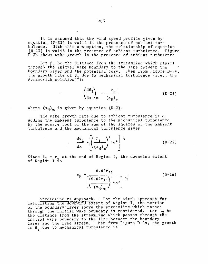
203

It is assumed that the wind speed profile given by equation C3~.32) is' -valid in the presence of ambient tur­bulence. With this assumption, the relationship of equation (D~23) is -valid in the presence of ambient turbulence. Figure D-2b shows wake growth in the presence of ambient turbulence.

Let B1 be the distance from the streamline which passes through th~ initial wake boundary to the line between the boundary layer and the potential core, Then from Figure D-2a, the growth rate of 81 due to mechanical turbulence (i.e., the Abramovich solut.ion) is

(D-Z4)

where (xH)m is given by equation (D~2).

The wake growth rate due to ambient turbulence is a. Adding the ambient turbulence to the mechanical turbulence by the square root of the sum of the squares of the ambient turbulence and the mechanical turbulence gives

(D-Z5)

Since 61 = r at the end of Region I, the downwind extent of Region I is

0.6Zr Zl (D-Z6)

Streamline rz ap~roach. - For the sixth approach for calculating the downwlnd extent of Region I, the portion of the boundary layer above the streamline which passes through the initial wake boundary is considered. Let S2 be the distance from the streamline which passes through tfie initial wake boundary to the line between the boundary layer and the free stream. Then from Figure D-2a, the growth in 82 due to mechanical turbulence is

204

( d~Z) = dx m

(D-27)

Adding ambient turbulence in the manner described above gives

Since

d6 Z dx

the downwind extent of Region I is

0.38r Z1

(D-Z8)

(D-Z9)

(D- 30)

0.5r21 approach. - For the seyenth approach for calculat­ing the downwind extent of Region I, the boundary layer is assumed to develop about a line which bisects the boundary layer. The boundary layer is assumed to develop equally on both of its sides. In this case

(D- 31)

In this case, the line connecting the initial wake boundary and r at the end of Region I is not a streamline. The downwInd extent of Region I is developed in the same manner as presented above for the previous two approaches. The results are identical for development based on 61 or on 6Z above because in this case 61 = 6z. For both cases,

(D-3Z)

205

It is noted that multiplication of the numerator and denominator of the right side of equation ~~32) gives the identical result given by equations (D-IZ) and CD~13). Therefore, the b approach II and the 0.5r Z1 approach are mathematically identical.

Comparison of Results

Figure D-3 shows the donwwind extent of Region I as a function of a, the wake growth rate due to ambient turbulence, for the first four approaches presented above. For Figure D-3, m = 3. Figure D-4 shows similar data for the last three approaches for calculating the downwind extent of Region I. For Figure D~4, m = 3. Figures D-5 and D-6 show information similar to that shown in Figures D-3 and D~4, respectively, but for m = 2. As mentioned previously, approaches 4 and 7 are mathematically identical.

Approaches 3 and 4 are identical, except that approach 3 augments the Abramovich solution for a, whereas approach 4 augments the Abramovich solution for Za. From a physical point of ' view, the 2a approach is more reasonable than the a approach because ambient turbulence affects the growth of the boundary layer on both sides of the boundary layer.

In Region I, mass continuity demands that the flow have an inward radial component. This is illustrated by the fact that the streamline which passes through the inti tal wake radius has an inward component. For approaches 1 and Z, the wake growth rate is taken relative to the line r = r , which has no physical relationship to the flow direc~ion or to the boundary layer. Relative to the flow and to the boundary layer, the line r = rO is a randomly drawn line. From a physical point of view, the measurement of the growth of the boundary layer from the streamline or from the line which bisects the boundary layer is more plausible.

For these reasons, from a physical point of view, approaches 4, 5, 6, and 7 are the most plausible approaches for the calculation of the downwind extent of Region I. Figures D-4 and D~6 show that the results do not vary greatly between these approaches (recalling that approach 4 is mathematically identical to approach 7). For these reasons, approaches 4 and 7 were chosen as the approaches for calculating the downwind extent of Region I in the model.

Z06

r Zl --~---I

Potential core

Downwind coordinate, x

Potential core

Downwind coordinate, x

Potential core

Downwind coordinate, x

I - -iro

® I

I I I I I

Zl

Figure D-l. - Angle used from Abramovich model to be augmented for ambient turbulence and used to calculate downwind extent of Region I

207

m = 3 2

Free stream ~ ~ ___ ~f21~O~W~-:-__ ------}--- r 21

]" r: ~-_S~:::~ __ St-2 --rs

ro layer ~

~ Potential Sl ~ ro

:s: core

2 4 6 8 10 12 14

Distance downwind of turbine, x

(a) Region I for Abramovich solution (no ambient turbulence)

xH

(b) Region I with ambient turbulence

Figure D-2. Geometry of Region I of the wake.

~

.,..;

.,..; "t:l

CIS H

H 0 ~ 0 H

'--'

"t:l 0:::

.......... ::r:

><

H

s:: 0

'''';

0.0 (!)

p::

lH 0

~

s:: (!) ~

>< (!)

"d s::

'''';

~ s:: ~ 0

Cl

14

] 2

10

8

6

4

Z

o 0

208

~ \'\.~ \ '\,

\" '\.~,~ "" "-.~ , " "'-.~ .. '" "--- _______ b

............... -- -- approach I

__ -...... r 1 approach

-- b approach II

0.3 0.4

Wake growth Tate due to ambient turbulence, ex

r z approach

Figure D-3. - Comparison of first four approaches for calculating xH for m = 3.

14

::r: ><

1Z ~

::: 0 . ..., 10 b.()

a.> ~

8 ~ 0

.j.J

::: 6 a.> .j.J

>< a.>

4 '"d ::: . ..., ~ Z ::: ~ 0

q

00

~

~\ \\ \\ \\

"" "" " ........... "

Z09

Streamline "' ----~ --_ r 1 approach ---- -------_ ---- 0.5r Z1 approach

\:.......Streaml ine r Z approach

O.Z 0.3

Wake growth rate due to ambient turbulence, a

0.4

Figure D-4. - Comparison of last three approaches for calculating xH for m = 3.

H

210

20

18~ \ \'

:: \ \\ \ \ \

\\\ \ \ \

\\~ \" " '''-,-""'-.....~~

" '-----......... _______ b approach I

. ,,---- ------__ --- r 1 approach ---______________ --__ -- b approach II r Z approach

12 .

1

8

Z

°o~--~~~--~--~----~--~---L--~---0.3 0.4

Wake growth rate due to ambient turbulence, :x

Figure D-S. - Comparison of first four approaches for calculating xH for m = 2.

::c ><

H

~ 0

0.-1 co Q)

IX

4-1 0

.j.J

~ Q)

.j.J

>< Q)

"d ~

0.-1 :s: ~ :s: 0 ~

20

18

16

14

12

10

8

6

4

Z

\~ ~ \\ \\ \ " \\ ~"

211

"" "-', .. Streamline "-- .................... r 1 approach

~----------__ --0.5 r Z1 approach

c:= Streamline

00 ~ __ ~ __ ~~ __ ~ __ ~~~~ __ ~~ __ ~ __ ~~ r Z approach

0.1 0.4 Wake growth rate turbulence, a.

to

Figure D-6. - Comparison of last three approaches for calculating xH for m = 2.

1. Report No. I 2. Government Accession No. 3. Recipient's Catalog No.

NASA CR-165380 4. Title and Subtitle 5. Report Date

WIND FLOW CHARACTERISTICS IN THE WAKES OF LARGE September 1981 WIND TURBINES 6. Performing Organization Code

VOLUME I - ANALYTICAL MODEL DEVELOPMENT C-41119-D 7. Author(s) 8. Performing Organization Report No.

W. R. Eberle LMSC-LOREC DOOOO08 10. Work Unit No.

9. Performing Organization Name and Address

Lockheed Missiles and Space Company, Inc. Huntsville, Alabama 11. Contract or Grant No.

DEN 3-29 13. Type of Repon and Period Covered

12. Sponsoring Agency Name and Address Contractor Report U. S. Department of Energy Division of Wind Energy Systems 14. Sponsoring Agency ~.Report No.

Washington, D. C. 20545 DOE/NASA/0029-1

15. Supplementary Notes Final Report. Prepared under Interagency Agreement EX-76-I-01-1028. Project Manager, Joseph M. Savino, Wind Energy Project Office, NASA Lewis Research Center, Cleveland, Ohio 44135.

16. Abstract

As part of the DOE/NASA research program on wind energy, a computer program to calculate the wake downwind of a wind turbine was developed. Turbine wake characteristics are useful for determining optimum arrays for wind turbine farms. The analytical model is based on the characteristics of a turbulent coflowing jet with modification for the effects of atmospheric turbulence. The program calculates overall wake characteristics, wind profiles, and power recovery for a wind turbine directly in the wake of another turbine, as functions of distance downwind of the turbine. The calculation procedure is described in detail, and sample results are presented to illustrate the general behavior of the wak~ and the effects of principal input parameters.

17. Key Words (Suggested by Author(s)) 18. Distribution Statement Wind turbine Unclassified - unlimited Wake flow STAR Category 44 Turbine farms DOE Category UC-60

19. Security Classif. (of this report! 120. Security Classif. (of this page) 21. No. of Pages 1 22. Price'

Unclassified Unclassified

• For sale by the National Technical Information Service, Springfield, Virginia 22161

,:, U.S. GQYEANMENT PRINTING OFFICE: 1981-757-07Z/3210

End of Document