Probabilistic modeling of S-N curves

Remy Fouchereau, Gilles Celeux, Patrick Pamphile

To cite this version:

Remy Fouchereau, Gilles Celeux, Patrick Pamphile. Probabilistic modeling of S-N curves. 2014.<hal-00924080>

HAL Id: hal-00924080

https://hal.inria.fr/hal-00924080

Submitted on 6 Jan 2014

HAL is a multi-disciplinary open accessarchive for the deposit and dissemination of sci-entific research documents, whether they are pub-lished or not. The documents may come fromteaching and research institutions in France orabroad, or from public or private research centers.

L’archive ouverte pluridisciplinaire HAL, estdestinee au depot et a la diffusion de documentsscientifiques de niveau recherche, publies ou non,emanant des etablissements d’enseignement et derecherche francais ou etrangers, des laboratoirespublics ou prives.

Probabilistic modeling of S-N curves

corresponding author : Remy Fouchereaua,c, +33672330781

fouchereau.remy@gmail.com

Gilles Celeuxb, Gilles.Celeux@inria.fr

and Patrick Pamphilea, patrick.pamphile@math.u-psud.fr

aLabo de mathmatiques, Universite Paris-Sud 11, 91405 Orsay, FrancebSelect, Inria, 91405 Orsay, France

cSafran-Snecma, France

November 22, 2013

Abstract

S-N curve is the main tool to analyze and predict fatigue lifetimeof a material, component or structure. But, standard models based onmechanic of rupture theory or standard probabilistic models for ana-lyzing S-N curves could not fit S-N curve on the whole range of cycleswithout microstructure information. This information is obtained fromcostly fractography investigation rarely available in the framework ofindustrial production. On the other hand, statistical models for fatiguelifetime do not need microstructure information but they could not beused to service life predictions because they have no material interpre-tation. Moreover, fatigue test results are widely scattered, especiallyfor High Cycle Fatigue region where split S-N curves appear. This isthe motivation to propose a new probabilistic model. This model isa specific mixture model based on a fracture mechanic approach, anddoes not require microstructure information. It makes use of the factthat the fatigue lifetime can be regarded as the sum of the crack initi-ation and propagation lifes. The model parameters are estimated withan EM algorithm for which the maximisation step combines Newton-Raphson optimisation method and Monte Carlo integrations. The re-sulting model provides a parsimonious representation of S-N curveswith parameters easily interpreted by mechanic or material engineers.This model has been applied to simulated and real fatigue test datasets. These numerical experiments highlight its ability to produce agood fit of the S-N curves on the whole range of cycles.

Keywords: S-N curves, Lognormal Distributions, Mixture, ConvolutionProduct, EM algorithm, Quantile Estimation

1

1 Introduction

A fatigue failure occurs when a component is subject to a repeated stressover a long period of time. Fatigue failures are all the more dangerous sincethey can occur for stress not higher than the service loading. In aeronau-tic industry, fatigue is the most common reason of breaking for mechanicparts. Fatigue failure analysis is an important issue for reliability analysisand structures design in many domains such as power generation industry,automotive industry and transportation, construction industry, civilian ormilitary engineering.

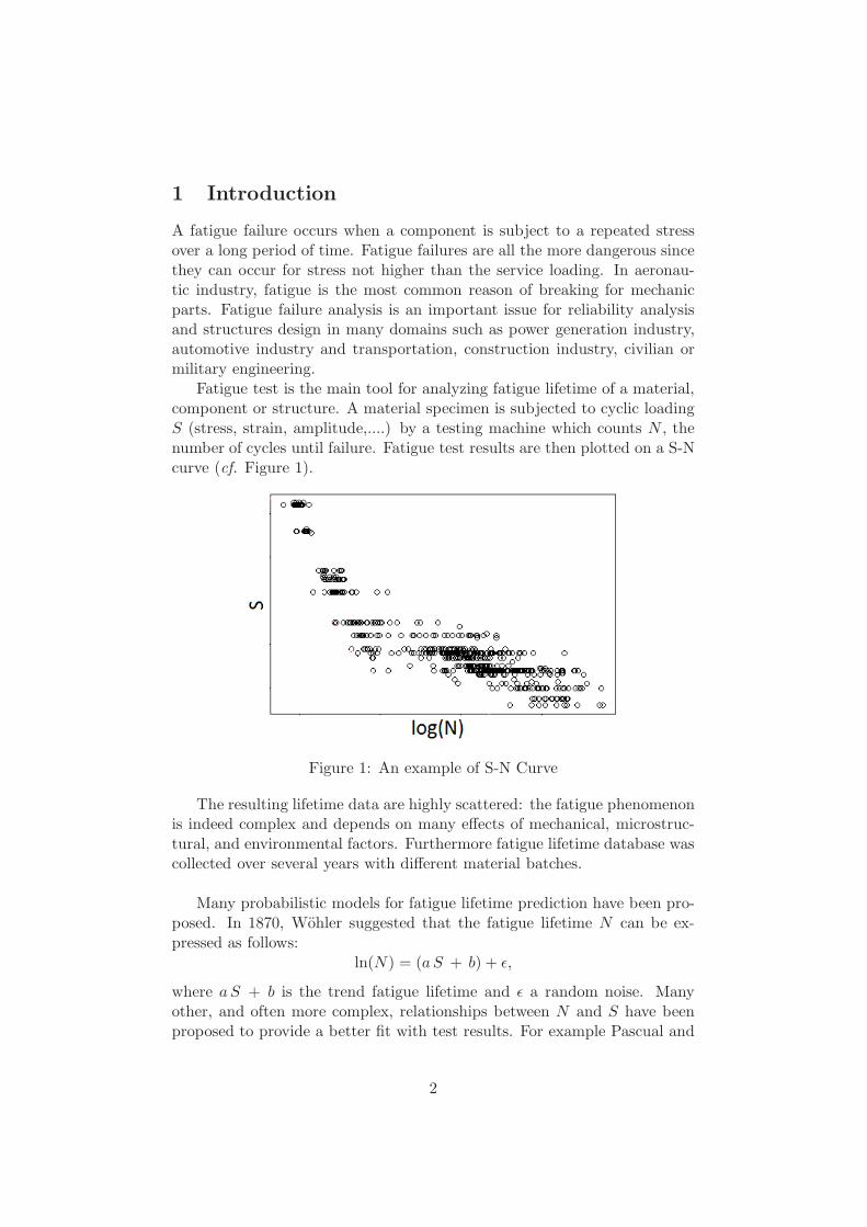
Fatigue test is the main tool for analyzing fatigue lifetime of a material,component or structure. A material specimen is subjected to cyclic loadingS (stress, strain, amplitude,....) by a testing machine which counts N , thenumber of cycles until failure. Fatigue test results are then plotted on a S-Ncurve (cf. Figure 1).

Figure 1: An example of S-N Curve

The resulting lifetime data are highly scattered: the fatigue phenomenonis indeed complex and depends on many effects of mechanical, microstruc-tural, and environmental factors. Furthermore fatigue lifetime database wascollected over several years with different material batches.

Many probabilistic models for fatigue lifetime prediction have been pro-posed. In 1870, Wohler suggested that the fatigue lifetime N can be ex-pressed as follows:

ln(N) = (aS + b) + ǫ,

where aS + b is the trend fatigue lifetime and ǫ a random noise. Manyother, and often more complex, relationships between N and S have beenproposed to provide a better fit with test results. For example Pascual and

2

Meeker [15] proposed the following model:

ln(N) = a− b× log(S − S0) + ǫ,

where S0 is an unknown random variable that stands for the fatigue limit.For industrial application, data are widely scattered due to variability in thecrack mechanism and its synergism with fatigue. However models mentionedabove do not deal with crack mechanism, thus they cannot provide a goodfit on the overall SN curve.

Moreover, recent fatigue studies reported that for High Cycle FatigueRegion (HCF: 104 < N ≤ 107), a ”duplex SN curve” occurs ([17],[10]).Deterministic and probabilistic approaches have been proposed to take intoaccount this phenomenon.

Deterministic models are based on the fracture mechanic theory. Thosemodels involve microstructure parameters which can explain the S-N curveduality: crack nucleation in surface/subsurface, crack growth rate for small-crack/large-crack, ...(cf.[18],[4]). Unfortunately, those models could not beused without costly microstructure investigation involving a scanning elec-tron microscope. Fractography analysis is not completed for the whole col-lection of industrial data. In addition, microstructure parameters are diffi-cult to be accurately estimated.

Probabilistic approach make use of competing risk models ([16],[5]) ormixture models ([12], [8]). Components of competing risk, or mixture mod-els, are connected to fatigue mechanisms: crack nucleation surface/subsurface,etc. Yet again, those components are pre-identified through costly mi-crostructure analysis of the material or the fracture. Therefore, those meth-ods are both difficult to be used for industrial production where microstruc-ture analysis are rarely done.

Alternative probabilistic models fit the data without using microstruc-tural or mechanical information. Those models are data dependent and thuscannot be employed for service life predictions.

We propose a mixture model based on the fracture mechanism, andwhich do not require fractography investigations. This model exploits thefact that the fatigue can be regarded as the sum of the crack initiation lifeand the crack propagation life. The initiation lifetime, Ni, may be definedas the number of cycles required to form a small crack (of the order of thematerial grain size). The propagation lifetime, Np, is the number of cyclesrequired to extend the crack from this small crack size to the critical sizeat which fracture occurs. Thus, a fatigue test lifetime can be written asN = Np when a crack appears at the first load or N = Np + Ni otherwise

3

(cf. [1]). This behavior leads to the mixture model

fN = π(S)fNp + (1− π(S))fNi+Np , (1)

π(S) being the probability of having a crack initiation at the first load ofS. Since the crack mechanism (propagation with or without initiation) isunknown, the model parameters are estimated through the Expectation-Maximisation algorithm (cf. [6]).The paper is organized as follows. In Section 2, we propose a mixturemodel based on a statistical analysis of fatigue data and detail its parametricform. In Section 3, the maximum likelihood estimate of the mixture modelparameters is presented through the EM algorithm. Numerical experimentsfrom simulated data and from the collection of real data under study arepresented in Section 4. Some concluding remarks are given in Section 5,while technical points are postponed to Appendix A.

2 The Initiation-Propagation Mixture model

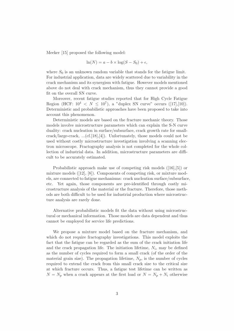
The proposed model has been inspired by the analysis of fatigue data fromindustrial production. Figure 2 represents the QQ-plot of these fatigue dataagainst a lognormal distribution.

Figure 2: QQ-plots of the empirical distribution of N vs. a log-normaldistribution as a function of S

Each symbol represents a different stress level. For high stress, a singlelognormal fits well the data: the corresponding QQ-plot is adjusted with aline. The same observation can be made for the lowest stress. For mediumstresses, broken-line QQplots indicate an underlying mixture of two distri-butions. Moreover the proportion of the two mixture components vary withthe stress: for high and low levels, a single component is present, while thereare two components for medium stress levels.

4

The question is to understand where these two components come from.If we refer to [1], the lifetime can be decomposed into two components:

• Ni: the crack initiation period,

• Np: the crack propagation period.

For high stress levels, at the first load, a small crack appears. Thus there isno initiation. On the contrary the propagation lifetimes can be seen at allstress levels. Finally a fatigue lifetime can be written as

N =

{

Np if Z = 1

Ni +Np if Z = 0

where Z denotes the label for an initiation at the first load (Z = 1 if thecrack starts at the first cycle, Z = 0 otherwise).

In most industrial fatigue databases, the values of the Z are not available.From figure 2, it is reasonable to assume that Ni and Np follow lognormaldistributions.

fNi(n, s) =

1

nσi√2π

exp

(

− [ln(n)− (αi s+ βi)]2

2σ2i

)

; (2)

fNp(n, s) =1

nσp√2π

exp

(

− [ln(n)− (αp s+ βp)]2

2σ2p

)

, (3)

s being the stress level of the test. The resulting fatigue lifetime is assumedto be a mixture of the propagation lifetime, Np, and the total lifetime Ni +Np. Its density function is

fN = π(s) fNp + (1− π(s))fNi+Np , (4)

π being the probability that a crack initiation occurs at the first load.The term Ni+Np, represents the standard fatigue behavior, whereas the

first term Np represents an unusual fatigue behavior of ”pure propagation”.The proportion of each component varies with s, and it is to assumed thatπ is linked with s by a logistic regression

π(s) =eα+βs

1 + eα+βs.

Obviously, it is important to prove the identifiability of this model whichensures that a unique optimal set of (4) parameters can be fitted on fatiguedata. This is done in Appendix A.

5

3 Estimation of the model parameters

Since we do not known if an crack initiation took place on first load orafter, this model is a missing structure data model. Thus the parametersof model (4) are estimated with the Expectation-Maximisation algorithm(EM, see [6]). The maximization step of the EM algorithm is here difficult,since the expectation of the complete log-likelihood knowing the fatiguedata involves a complex non linear function of the parameters. It requiresan integral computation through Monte Carlo simulations. In addition themaximization step is achieved by using the Newton-Raphson algorithm.Let θ = (θp, θi, α, β) be the vector of parameters of the model (4), withθp = (ap, bp, σp) and θi = (ai, bi, σi). The algorithm EM is a two stepalgorithm maximizing the observed likelihood:

L(N,S ; θ) =

m∏

k

f(N,S)(nk, sk ; θ). (5)

knowing the data (N,S) and a current value of the parameters. The EMalgorithm is making use of the complete likelihood

L(N,S,Z ; θ) =m∏

k

f(N,S,Z)(nk, sk, zk ; θ), (6)

where Z denotes the missing origin of the crack: Z = 1 if the crack startsat the first load, and Z = 0 otherwise. Then

f(N,S,Z)(n, s, z ; θ) = (π(s)[fNi(n, s)])z × ((1 − π(s))[fNi+Np(n, s)])

(1−z).

Since the indicator variable Z is not observed, the complete likelihoodL(N,S,Z ; θ) cannot be maximized directly. The Expectation step consistsof computing the expected value of the completed likelihood knowing thedata (N,S) and a current value of the parameters [6].

The EM algorithm Starting from a vector parameter θ(0) = (θ(0)p , θ

(0)i ;α(0), β(0)),

this algorithm iterates the E and M steps.

1. E step: computation of the expected complete loglikelihood knowinga current parameter θ(j) :

Q(θ|θ(j)) = E[

lnL(N,S,Z ; θ) |(Z|N ; θ(j))]

=

m∑

k

[

tk ln(fNp(nk, sk ; θp))

+(1− tk) ln(fNi+Np(nk, sk ; θ))]

;

(7)

6

tk being the conditional distribution of Z:

tk = E[Z|N,S; θ(j)]

= P(Z = 1|N = nk, S = sk ; θ = θ(j))

=π

(r)(sk)fNp(nk; sk, θ

(r)

p )∑

l=(i,p)

πl(sk)φl(nk; sk, θ(r));

where φl stands for fNp if l = 1, and fNi∗ fNp otherwise.

2. M step: maximization of Q(θ|θ(j))

θ(j+1) = argmaxθ

Q(θ|θ(j)).

It can be decomposed in two independent maximisations

• maxα,β

N∑

k=1

tk ln(π(sk)) + (1− tk) ln(1− π(sk));

• maxθ

N∑

k=1

tk ln(fNp(nk, sk, θp)) + (1− tk) ln(fNi∗ fNp(nk; sk, θ));

which can be achieved with a Newton-Raphson algorithm.

The sequence θ(1), θ(2),... generated by EM is expected to convergetoward a local maximum of the observed-data likelihood L(N,S ; θ)under fairly general conditions (cf. [6]).

The solution provided by EM could be highly dependent of the initial pa-rameter values. It appears not for the initiation-propagation mixture modeland the following initial values provide satisfactory parameter estimates.

• π(0) = 0.5;

• θ(0) = (θ(0)p , θ

(0)i ) has been derived from a clusterwise linear regression

on the log-lifetimes (cf. [7]). For LCF region(N < 104) N ≃ Np,whereas for VHCF region N ≃ Ni. Then clusterwise regression pro-vides quickly an honest initial estimation of the model parameters andthe EM algorithm converges a sensible local maximum.

The maximization of Q(θ|θ(j)) requires a Newton-Raphson algorithmcombined with a Monte Carlo algorithm to evaluate the density of fNi+Np

which is now described.The convolution product

fNi+Np(n) =

∫ n

0fNi

(n− x)fNp(x)dx (8)

7

used in (7) does not lead to a closed form expression. Using a Gauss-Legendre Quadrature would not be efficient here, because for some x valuesthe function to be integrated is highly picked. This is why a Monte Carloapproximation has been used and is now described. The integral can bewritten

fNi+Np(n) =

∫ n

0fNi

(n − x)fNp(x)dx (9)

= ENp [fNi(n−Np)

+] (10)

= ENi[fNp(n−Ni)

+]. (11)

It is then approximated by importance sampling using either (10), either(11), according to σ(Np) < σ(Ni) or not. Without loss of generality assum-ing that σ(Np) < σ(Ni) the procedure is as follows:

1. b independents replications of fNp are simulated: npj , j = 1, · · · , b. Inpractice, b = 1000 appears to provide satisfactory results.

2. using (10), fNi+Np(n) is estimated by

fNi+Np(n) =1

b

b∑

j=1

fni(n− npj)

+.

Dealing with censored data Often fatigue data are right censored, thelikelihood includes also the probability P(N > c). Since this probability isdifficult to compute, two alternative solutions are proposed:

a. using an asymptotic approximation (cf [2]), we have

P(N > c) ∼ π2σie− 1

2

(log(c)−µi)2

σ2i

√2π(log(c) − µi)

.

But an asymptotic approximation is not realistic when censoring oc-curs at low stress levels.

b. simulating the data over the censorship c, the EM algorithm is replacedby the Stochastic EM algorithm (cf [3]). But, simulate values greaterthan c, could take a huge computation time.

In order to circumvent the mentioned numerical problems, we make use ofthe following hybrid heuristics which provides good results in practice.

• Each censored data is assumed to arises from the component withdensity fNi+Np(n) and thus tk1 = 0.

8

• Before each M-step, for each censored data, simulate at most one hun-dred times the two lognormal distributions and sum them:

– if one of the 100 resulting values is greater than the censorship,consider this simulated value as an observed value in the M step;

– otherwise, the censorship is considered to belong to the distribu-tion tail and the asymptotic approximation above can be used.

4 Numerical experiments

4.1 Simulated data experiments

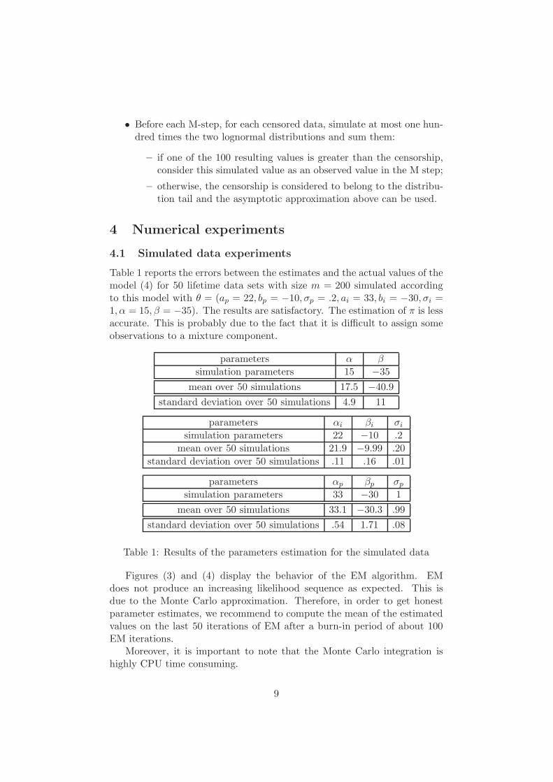
Table 1 reports the errors between the estimates and the actual values of themodel (4) for 50 lifetime data sets with size m = 200 simulated accordingto this model with θ = (ap = 22, bp = −10, σp = .2, ai = 33, bi = −30, σi =1, α = 15, β = −35). The results are satisfactory. The estimation of π is lessaccurate. This is probably due to the fact that it is difficult to assign someobservations to a mixture component.

parameters α β

simulation parameters 15 −35

mean over 50 simulations 17.5 −40.9

standard deviation over 50 simulations 4.9 11

parameters αi βi σisimulation parameters 22 −10 .2

mean over 50 simulations 21.9 −9.99 .20

standard deviation over 50 simulations .11 .16 .01

parameters αp βp σpsimulation parameters 33 −30 1

mean over 50 simulations 33.1 −30.3 .99

standard deviation over 50 simulations .54 1.71 .08

Table 1: Results of the parameters estimation for the simulated data

Figures (3) and (4) display the behavior of the EM algorithm. EMdoes not produce an increasing likelihood sequence as expected. This isdue to the Monte Carlo approximation. Therefore, in order to get honestparameter estimates, we recommend to compute the mean of the estimatedvalues on the last 50 iterations of EM after a burn-in period of about 100EM iterations.

Moreover, it is important to note that the Monte Carlo integration ishighly CPU time consuming.

9

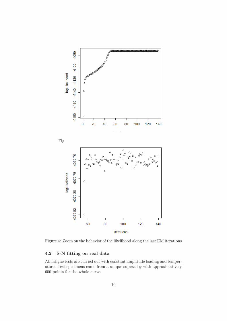
Figure 3: Behavior of the likelihood along the EM iterations

Figure 4: Zoom on the behavior of the likelihood along the last EM iterations

4.2 S-N fitting on real data

All fatigue tests are carried out with constant amplitude loading and temper-ature. Test specimens came from a unique superalloy with approximatively600 points for the whole curve.

10

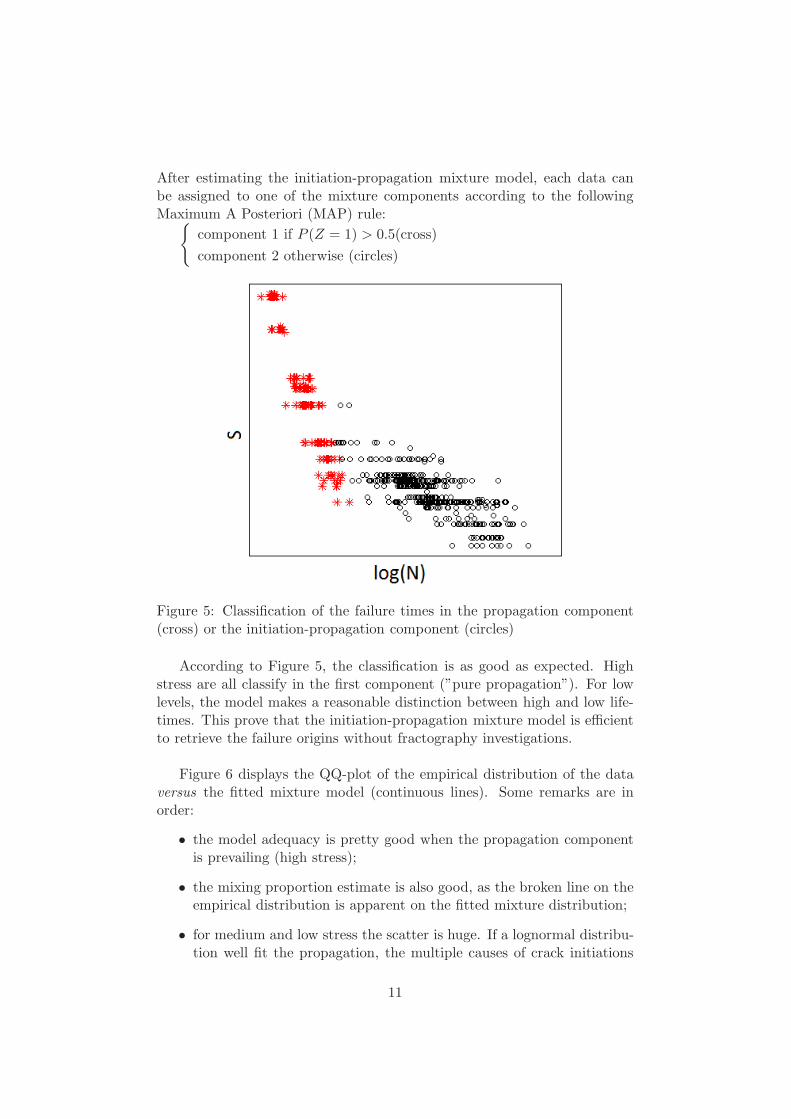
After estimating the initiation-propagation mixture model, each data canbe assigned to one of the mixture components according to the followingMaximum A Posteriori (MAP) rule:

{

component 1 if P (Z = 1) > 0.5(cross)

component 2 otherwise (circles)

Figure 5: Classification of the failure times in the propagation component(cross) or the initiation-propagation component (circles)

According to Figure 5, the classification is as good as expected. Highstress are all classify in the first component (”pure propagation”). For lowlevels, the model makes a reasonable distinction between high and low life-times. This prove that the initiation-propagation mixture model is efficientto retrieve the failure origins without fractography investigations.

Figure 6 displays the QQ-plot of the empirical distribution of the dataversus the fitted mixture model (continuous lines). Some remarks are inorder:

• the model adequacy is pretty good when the propagation componentis prevailing (high stress);

• the mixing proportion estimate is also good, as the broken line on theempirical distribution is apparent on the fitted mixture distribution;

• for medium and low stress the scatter is huge. If a lognormal distribu-tion well fit the propagation, the multiple causes of crack initiations

11

are badly taken into account with a single lognormal distribution.

Figure 6: QQ-plot with model approximation

An important question to be answered when modeling fatigue lifetime is toprovide good estimates of extreme quantiles on the whole range of stressvalues. Using the estimated initiation-propagation mixture model, a 0.1%-quantile has been designed from the simulation of 106 lifetimes according tothe estimated distribution. The resulting quantile is displayed in figure (7).It appears to be quite satisfactory since one of the 600 observed data is be-yond this 0.1%-quantile. It means that the initiation-propoagation mixturemodel provides a useful estimation of the fatigue lifetime on the whole rangeof stress values.

5 Conclusion

Fatigue tests and the resulting S-N curve, are the main basic tools for analyz-ing and predicting fatigue lifetime of a material, component, or structure.S-N curves are in general widely scattered, and therefore service lifetimepredictions are difficult. For instance, a ”duplex behavior” appears in theS-N curves of High Cycle Fatigue region. This ”duplex behavior” can some-times be characterized by costly fractography investigations. In an indus-trial framework, fractography investigations are not completed after eachtest, and standard prediction models cannot be used. We have proposed amixture model based on the fracture mechanism, without fractography in-formation. This is a latent structure model and its parameters are estimated

12

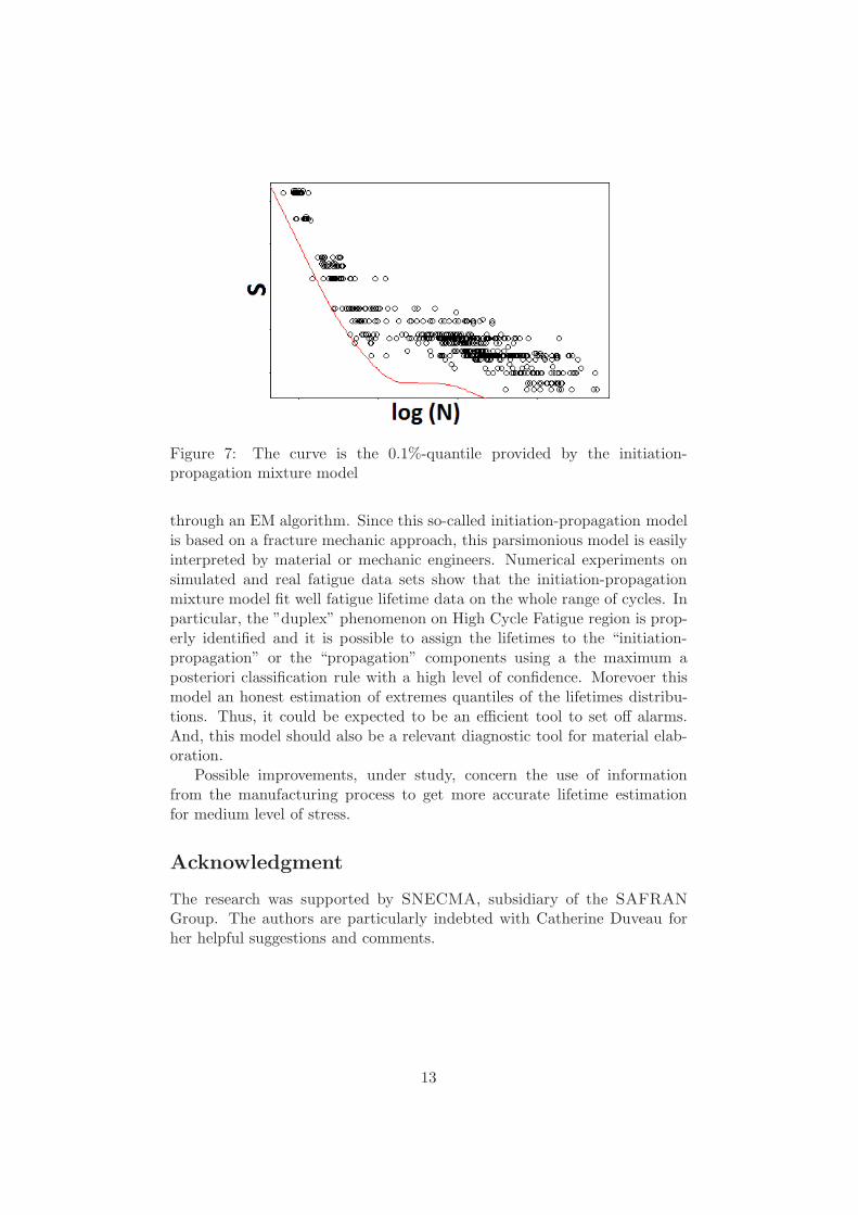
Figure 7: The curve is the 0.1%-quantile provided by the initiation-propagation mixture model

through an EM algorithm. Since this so-called initiation-propagation modelis based on a fracture mechanic approach, this parsimonious model is easilyinterpreted by material or mechanic engineers. Numerical experiments onsimulated and real fatigue data sets show that the initiation-propagationmixture model fit well fatigue lifetime data on the whole range of cycles. Inparticular, the ”duplex” phenomenon on High Cycle Fatigue region is prop-erly identified and it is possible to assign the lifetimes to the “initiation-propagation” or the “propagation” components using a the maximum aposteriori classification rule with a high level of confidence. Morevoer thismodel an honest estimation of extremes quantiles of the lifetimes distribu-tions. Thus, it could be expected to be an efficient tool to set off alarms.And, this model should also be a relevant diagnostic tool for material elab-oration.

Possible improvements, under study, concern the use of informationfrom the manufacturing process to get more accurate lifetime estimationfor medium level of stress.

Acknowledgment

The research was supported by SNECMA, subsidiary of the SAFRAN

Group. The authors are particularly indebted with Catherine Duveau forher helpful suggestions and comments.

13

References

[1] Alexandre, F. (2004) Aspects probabilistes et microstructuraux del’amorcage des fissures de fatigue dans l’alliage INCO 718. Phd thesis.Ecole Normale Superieure des Mines de Paris.

[2] Asmussen, S. and Rojas-Nandayapa, L. (2005), Sums of dependent log-normal random variables: asymptotics and simulation. Research report,Thiele Centre for Applied Matematics in Natural Science

[3] Celeux, G. and Diebolt, J. (1985) The sem algorithm: a probabilisticteacher algorithm derived from the em algorithm for the mixture prob-lem. Computational Statistics Quaterly, 2, 73-85.

[4] Chan, K.W. (2010), Role of microsture in fatigue crack initiation. Inter-national Journal of Fatigue, 32, 1428-1447.

[5] Crowder, M. (1999) Classical Competing Risks. Harlow, England:

Addison-Wesley

[6] Dempster, A.P., Laird N.M. and Rubin, D.B. (1977) Maximum Likeli-hood from Incomplete Data via the EM Algorithm. Journal of the Royal

Statistical Society.

[7] DeSarbo, W.S. and Cron, W.L. (1988) A maximum likelihood method-ology for clusterwise linear regression. International Journal of Classifi-cation, 5, 249-282.

[8] Harlow, D.G., Wei, R., Sakai,T. and Oguma, N. (2006), Crack growthbased probability modeling of S-N response for high strength stell. In-ternational Journal of Fatigue, 28 ,1479-1485.

[9] Hanaki, S., Yamashita, M., Uchida, H. and Zako, (2010) M. On stochas-tic evaluation of SN data based on fatigue strength distribution. Inter-national Journal of Fatigue, 32, 605-609.

[10] Jha, S.K. and Ravi Chandran, K.S. (2003), An unusual fatigue phe-nomenon: duality of the SN fatigue curve in the b-titanium alloyTi10V2Fe3Al. Scripta Materialia, 48, 1207-1212.

[11] Jha, S.K., Caton, M.J. and Larsen, J.M. (2007), A new paradigm offatigue variability behavior and implications for life prediction. Material

Science and Engineering :A, 468-470, 23-32.

[12] Jha, S.K., Larsen, J.M. and A.H. Rosenberg (2009), Toward a physics-based description of fatigue behaviour in probabilistic life-prediction.Engineering Fracture Mechanics, 76, 681-694.

14

[13] McLachlan, G. and Peel, D. (2000), Finite mixture models, Wiley.

[14] Nelson , W. (1982), Applied life data analysis, Wiley.

[15] Pascual, F.G. and Meeker, W.Q. (1999), Estimating Fatigue Curveswith the Random Fatigue-Limit Model. Technometrics, 41, 277-290.

[16] Ravi Chandran, K.S., Chang, P. and Cashman, G.T. (2010) Competingfailure modes and complex SN curves in fatigue of structural materialsInternational Journal of Fatigue, 32, 482-491.

[17] Sakai, T., Nakayasu, H. and Nishikawa, I. (2005) Establishment ofJSMS standard regression method of SN curves for metallic materials.Safety and Reliability of Engineering Systems and Structures, 643

[18] Shiozawa, K., Murai, M., Shimatani, Y. and Yoshimoto, T. (2010) Tran-sition of fatigue failure mode of NiCrMo low-alloy steel in very high cycleregime. International Journal of Fatigue, 32, 541-550.

15

Appendix A

This appendix is to devoted to prove the identifiability of the model

fN = π(s) fNp + (1− π(s))fNi+Np ,

under the realistic assumption for material lifetimes that σi > σp. It isdifficult to prove the identifiability in a single exercise and the proof is donestep by step.

1. At first, it is assumed that the mixing proportion π and the stresslevel s are fixed, and the uniqueness of the position and dispersionparameters µ and σ are proved for the two lognormal distributions.

2. Then by allowing the stress level s to vary, it is proved that the re-gression parameters a and b used to define µ are unique for the twolognormal distributions. Similarly the uniqueness of the parameters αand β, involved in the logistic regression model for the proportion π,are proved.

1: Assuming s and π fixed, under the assumption σi > σp, we have theasymptotic equivalence for the tail distribution of model (4), see [2]:

P(N > x) ∼ π2σie− 1

2

(log(x)−µi)2

σ2i

√2π(log(x)− µi)

.

Thus, if the distribution of N has two parameterizations (π1, π2 = 1 −π1, µi, σi, µp, σp) and (π′

1, π′2 = 1− π′

1, µ′i, σ

′i, µ

′p, σ

′p), we have

limx→∞

π2σi√2π(log(x)−µi)

e− 1

2

(log(x)−µi)2

σ2i

π′

2σ′

i√2π(log(x)−µ′

i)e− 1

2

(log(x)−µ′i)2

σ′2i

= 1.

That is

limx→∞

π2σi

π′2σ

′i

log(x)− µi

log(x)− µ′i

e− 1

2log2(x)( 1

σ2i

− 1

σ′2i

)− 12log(x)(− 2µi

σ2i

+2µ′i

σ′2i

)− 12(µ2iσ2i

−µ′2i

σ′2i

)

= 1

Since limx→∞

(

log(x)−µi

log(x)−µ′

i

)

= 1, it leads to

limx→∞

π2σi

π′2σ

′i

e− 1

2log2(x)( 1

σ2i

− 1

σ′2i

)− 12log(x)(− 2µi

σ2i

+2µ′i

σ′2i

)− 12(µ2iσ2i

−µ′2i

σ′2i

)

= 1.

16

A necessary condition to ensure this equation is that the term in log2(x) iszero, thus −1

2(1σi− 1

σ′

i) = 0 ⇒ σi = σ′

i. Then, the term in log(x) has to be zero

too and thus µi = µ′i. And, finally, it leads to lim

x→∞(π2π′

2) = 1 and thus π2 = π′

2.

To show the identifiability of the propogation parameter, we use theLaplace transformation L(fN ) =

∫ +∞0 estfN(t) dt of fN . We have

L(fN ) = π L(fNp) + (1− π)L(fNi)L(fNp),

L(fN ) = L(fNp)(π + (1− π)L(fNi)).

We have already shown that θi = θ′i, thus

L(fNp(n; θp))(π + (1− π)L(fNi)) = L(fNp(n; θ

′p))(π + (1− π)L(fNi

)),

which implies L(fNp(n; θp)) = L(fNp(n; θ′p)). If two variables have the same

Laplace transform, then they have the same distribution: fNp(n; θp) =fNp(n; θ

′p). Finally θp = θ′p since the lognormal distribution is identifiable.

2: For any stress level s, we have by definition of the model (4):

fN = π(s) fNp(n; s, µi(s), σi) + (1− π(s))fNi+Np(n; s, µi(s), µp(s), σi, σp),

with π(s) = eα+βs

1+eα+βs , µi(s) = ai + bis, and µp(s) = ap + bps.

For any s, we have proved that ap + bps = a′p + b′ps and ai + bis = a′i + b′is.It implies straightforwardly that ap = a′p, bp = b′p, ai = a′i and bi = b′i.

Similarly, for any s, we have eα+βs

1+eα+βs = eα′+β′s

1+eα′+β′s

and thus α = α′ and β = β′

�

17