Remuneration and Pensions

Calculation of

Intra-EU correction coefficients

in accordance with the EU Staff Regulations

Version: May 2016

Doc.A6465/14/59 rev3

Main Text

1

Preface

This document describes the calculation of correction coefficients applicable to the remuneration of staff

working in Intra-EU duty stations. Separate manuals describe the calculation of Extra-EU correction

coefficients1, and the index to monitor temporal evolution of consumer prices in headquarters duty

stations2. Another manual describes the calculation of specific indicators in accordance with Article 65 of

the Staff Regulations3.

These adjustments a direct component of the remuneration of EU staff and, by analogy, also affect many

other persons. They are therefore of great interest to many groups, including the Commission and other

Institutions, staff representatives, the Member States, other international organisations.

Eurostat therefore considers it important to provide a comprehensive document, where people interested

in this subject can find information on the legal background, on the basic principles and definitions and also

on details of the practical procedures concerning this issue.

This document is based on the Staff Regulations of Officials of the European Communities4 and other

relevant elements of the legal framework. The Working Group on Articles 64 and 65 is a platform for the

discussion of the methodology. It comprises Member States delegations and representatives of the

Commission and it is chaired by Eurostat.

As the remuneration system for EU officials and the methodological details for the calculation of correction

coefficients develop and evolve over time, this document has to be seen as a snapshot of the current state

of the art. It replaces all previous versions of this manual.

1 Document A6465/14/60

2 Document A6465/14/58

3 Document A6465/14/26

4 Council Regulation No 259/68 as modified most recently by Regulation (EU, Euratom) No 1023/2013 of the

European Parliament and of the Council of 22 October 2013

2

History

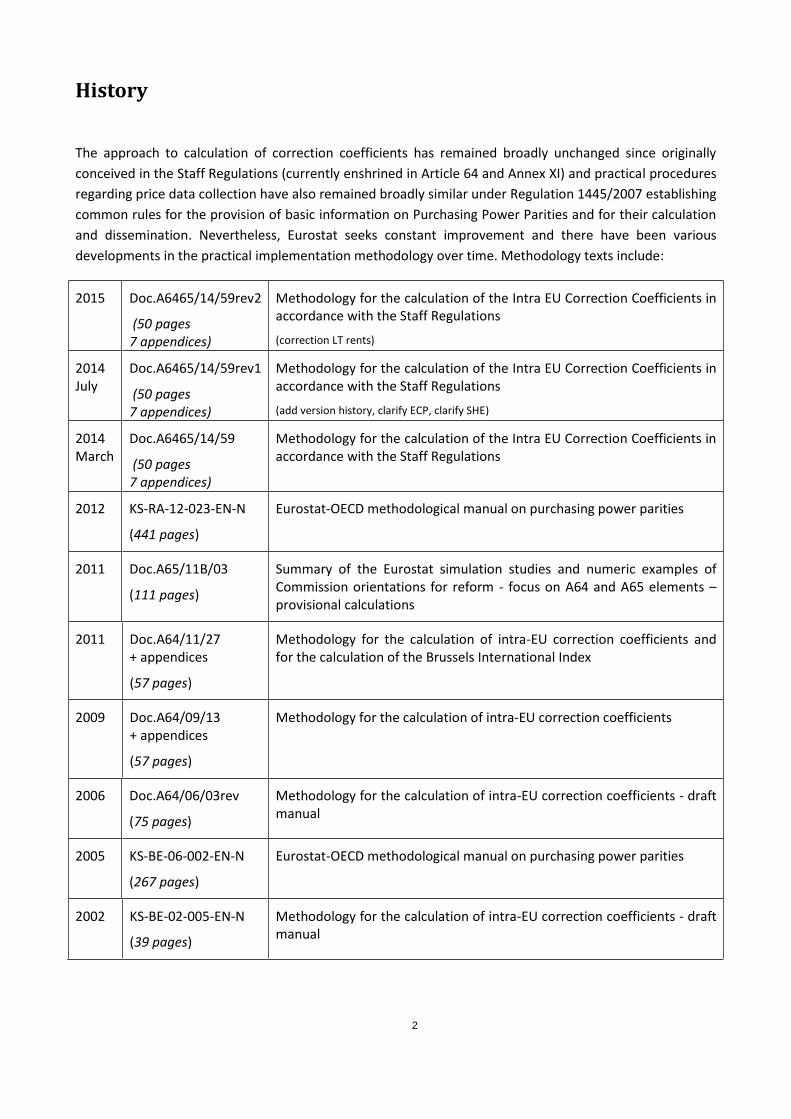
The approach to calculation of correction coefficients has remained broadly unchanged since originally

conceived in the Staff Regulations (currently enshrined in Article 64 and Annex XI) and practical procedures

regarding price data collection have also remained broadly similar under Regulation 1445/2007 establishing

common rules for the provision of basic information on Purchasing Power Parities and for their calculation

and dissemination. Nevertheless, Eurostat seeks constant improvement and there have been various

developments in the practical implementation methodology over time. Methodology texts include:

2015 Doc.A6465/14/59rev2

(50 pages 7 appendices)

Methodology for the calculation of the Intra EU Correction Coefficients in accordance with the Staff Regulations

(correction LT rents)

2014 July

Doc.A6465/14/59rev1

(50 pages 7 appendices)

Methodology for the calculation of the Intra EU Correction Coefficients in accordance with the Staff Regulations

(add version history, clarify ECP, clarify SHE)

2014 March

Doc.A6465/14/59

(50 pages 7 appendices)

Methodology for the calculation of the Intra EU Correction Coefficients in accordance with the Staff Regulations

2012 KS-RA-12-023-EN-N

(441 pages)

Eurostat-OECD methodological manual on purchasing power parities

2011 Doc.A65/11B/03

(111 pages)

Summary of the Eurostat simulation studies and numeric examples of Commission orientations for reform - focus on A64 and A65 elements – provisional calculations

2011 Doc.A64/11/27 + appendices

(57 pages)

Methodology for the calculation of intra-EU correction coefficients and for the calculation of the Brussels International Index

2009 Doc.A64/09/13 + appendices

(57 pages)

Methodology for the calculation of intra-EU correction coefficients

2006 Doc.A64/06/03rev

(75 pages)

Methodology for the calculation of intra-EU correction coefficients - draft manual

2005 KS-BE-06-002-EN-N

(267 pages)

Eurostat-OECD methodological manual on purchasing power parities

2002 KS-BE-02-005-EN-N

(39 pages)

Methodology for the calculation of intra-EU correction coefficients - draft manual

3

Table of Contents

PREFACE ............................................................................................................................ 1

HISTORY ............................................................................................................................. 2

I - INTRODUCTION .......................................................................................................... 5

II – THE EUROPEAN COMPARISON PROGRAMME (ECP) PRICE SURVEYS ....... 7

1. Introduction ....................................................................................................... 7

2. The surveys and the pre-survey work ............................................................... 8

3. Organisational aspects of price surveys ............................................................ 8

4. The price collection ......................................................................................... 10

5. Product specifications ..................................................................................... 11

6. Data processing ............................................................................................... 12

7. Review of consumer price surveys for Art.64 purposes ................................. 16

8. Treatment of missing values ........................................................................... 17

III – HEALTHCARE ........................................................................................................ 18

1. Introduction ........................................................................................................... 18

2. The new ECP approach to establish output-based measure for hospital care . 18

3. Integrating the new ECP data for A64 purposes ............................................. 19

IV - EDUCATION PARITIES ......................................................................................... 20

1. Introduction ........................................................................................................... 20

2. Approach for the Article 64 .................................................................................. 20

2.1 Cost data for European Schools ........................................................ 21

2.2 Cost data for national non-fee paying schools .................................. 21

2.3 Price data for fee paying Schools ...................................................... 21

2.4 Overall parity for Education.............................................................. 22

3. Practical issue ........................................................................................................ 22

V - ESTATE AGENCY RENT SURVEYS ..................................................................... 23

1. General remarks .............................................................................................. 23

2. The survey ....................................................................................................... 23

3. The questionnaire ............................................................................................ 24

4. Management of the survey .............................................................................. 27

VI - STAFF HOUSING SURVEY AND THE HOUSING INDICES ............................. 28

VII - CALCULATION OF RENT PARITIES ................................................................. 31

1. Introduction ..................................................................................................... 31

2. Moving average model .................................................................................... 31

3. Rent ratios ...................................................................................................... 34

4 Aggregation of rent ratios .............................................................................. 35

5. Checks and analyses ........................................................................................ 36

4

VIII - CONSUMPTION WEIGHTS – THE SURVEY OF HOUSEHOLD EXPENDITURE

(SHE)* ...................................................................................................................... 38

1. Introduction ..................................................................................................... 38

2. The SHE in Brussels ....................................................................................... 39

3. SHE for places of employment other than Brussels ....................................... 40

IX - CORRECTION COEFFICIENTS FOR OFFICIALS ............................................ 44

1. Introduction ........................................................................................................... 44

2. From price surveys to elementary parities ............................................................ 44

3. Calculation of the global parity ............................................................................. 46

4. Yearly update of the parities ........................................................................... 48

5. Intermediate adjustment ........................................................................................ 50

X – CORRECTION COEFFICIENTS FOR PENSIONERS ........................................... 51

Appendices

Appendix 1 List of 80 basic headings and 12 COICOP Groups

Appendix 2 Questionnaire for the Estate Agency Rent Survey in London

Appendix 3 EARS guideline for surveyors

Appendix 4a SHE questionnaire (paper format : Brussels)

Appendix 4b SHE questionnaire (paper format : Other Intra-EU staff)

Appendix 4c SHE questionnaire (paper format : Pensioners)

Appendix 4d SHE questionnaire (online)

Appendix 5 SHE glossary

Appendix 6a SHS Questionnaire (paper format)

Appendix 6b SHS Questionnaire (online)

Appendix 7 SHS instructions

Appendix 8 Price survey definition for fee-paying schools

NB. For the appendices, please see separate files.

5

I - INTRODUCTION

According to Annex XI of the Staff Regulations the adjustment of salaries of EU officials is determined by the following factors:

changes in the purchasing power of salaries of national civil servants in central government (Specific Indicator)5;

changes in the cost of living in Brussels and Luxembourg (Joint BELU Index);

economic parities between Brussels and the other duty stations in the Member States (Correction Coefficients)6.

The joint Belgium Luxembourg index (BELU index) is a Laspeyres-type index. Its aim, as stated in Annex XI of the Staff Regulation, is “to measure changes in the cost of living for officials of the Communities in Brussels” (Article 1.2 of Annex XI). The methodology used to calculate the BELU index is described in a separate document7.

Changes in the cost of living in places of employment other than Brussels and Luxembourg are derived indirectly from the value of the adjustment for Brussels and Luxembourg and changes in the economic parities between Brussels and those other places. The object of the economic parities is to compare the relative costs of living of European institution officials in Brussels (reference cities) and in each of the capitals and other duty stations where EU staff are serving.

The method used is to compare the price of a basket of goods and services purchased by the average official in Brussels with the price of the equivalent basket in each of the other duty stations. For this purpose, National Statistical Institutes (NSI) in co-operation with Eurostat carry out a number of price surveys (see chapter II). Since the collection of prices is time-consuming and expensive, the pricing of the full list of products is spread over a 3-year period with two surveys per year covering each one a broad category. Housing costs are treated differently from other prices for two reasons:

a) They are the largest single item of expenditure (at least 20–25% of total spending).

b) Housing is different from any other type of good or service because of its uniqueness. No two dwellings are alike, especially when one takes account of all the secondary attributes which affect the price, such as the quality of the district, access to shops, transport, schools and so on.

For these reasons and in view of the rapid fluctuations in the housing market, rent surveys are conducted every year and not every three years, as with the other items (see chapter III and IV).

5 The calculation of Specific Indicators in accordance with Article 65 of the Staff Regulations is described in a separate

manual. 6 The calculation of Correction Coefficients for Extra-EU duty stations in accordance with Annex X of the Staff

Regulations is described in a separate manual. 7 See doc.A6465/14/58

6

The total range of goods and services constituting the consumption of the average EU official is grouped into 80 basic headings for which a price ratio between Brussels and the duty station is calculated. The average of all the price ratios is called "economic parity" or Purchasing Power Parity (PPP). The overall economic parities, used for salary adjustment in duty stations other than Brussels and Luxembourg, are based on 80 elementary parities aggregated together using consumption weights.

For each place, the weights are estimated for each of the 80 basic headings and are expressed as percentages of total expenditure, according to their relative importance in the consumption basket. The weights normally reflect the expenditure pattern of the average EU official in each duty station.

To estimate expenditure patterns for EU officials, every five to seven years Eurostat carries out Surveys of Household Expenditure (SHE)8 in the different duty stations among the staff serving at that time; the average result is established as the consumption pattern of the duty station until the next survey. The purpose of these SHE is to determine the relative amounts of expenditure on different items of consumption. The methodology of the SHE is presented in chapter VI.

The ratio between the economic parity and the exchange rate (where applicable) used to pay the remuneration is called a correction coefficient. It operates as a percentage adjustment to salaries to take account of the cost differences between Brussels and the duty stations. The method of calculation is shown in chapter VII.

Since 2004, Staff Regulations also require the estimation of country economic parities for pensioners to “establish the equivalence of purchasing power of the pensions of officials paid in the Member States between each Member States with reference to Belgium”. The methodology is basically the same applied for the salaries; differences are explained in chapter VIII.

8 Formerly known as Family Budget Surveys (FBS)

7

II – THE EUROPEAN COMPARISON PROGRAMME (ECP) PRICE SURVEYS

1. Introduction

The price surveys, together with the rent surveys, form the basis of the calculations of the intra-EU correction coefficients (CC). The surveys are an essential part of the ‘European Comparison Program’ (ECP) and as such the preparation is crucial if any comparison between all participating countries is to take place. In short the results produced have to be comparable and therefore, the goods and services chosen for comparison need to be of similar standards. The prices used for the capitals are derived from the price surveys carried out by NSIs in the framework of the ECP, the coordination being ensured by Eurostat. For the other duty-stations similar surveys are carried out by Eurostat, assisted by the NSI. Price surveys used for the purpose of calculating the correction coefficient can, therefore, be divided in:

Price surveys conducted in the capitals as part of the ECP programme

The NSIs are responsible for the price collections in their countries. Furthermore it is their duty to ensure that the consumption pattern of the country is well represented among the products for which prices are collected. This means that an adequate number of representative consumer goods should be included in each product group. The price surveys are co-ordinated by Eurostat and the group leader countries (see section 3).

Price surveys conducted in other EU duty-stations outside the capitals

This point concerns the surveys conducted in Varese, Bonn, Karlsruhe and Munich. These surveys are the responsibility of Eurostat; but the NSIs assist and help Eurostat to validate the results.

The latter surveys are used only for the calculation of CCs; the methodology applied, the product definition and the timing is the same as for the surveys conducted in the capitals.

8

2. The surveys and the pre-survey work

Since the collection of prices is time-consuming and expensive, the pricing of the full list of products is conducted in a 3-year cycle, with two surveys every year, each covering a broad category of goods/services. At any point in time, there are several surveys in progress, each at different steps of the process (eg. item list definition, fieldwork preparation/coordination, results processing/validation). The price surveys for the calculation of CC's are representative of most of the goods and services consumed by EU-officials’ households. There are six product groups, with two surveys each year. They are:

Food, drinks and tobacco: food; non-alcoholic beverages; alcoholic beverages; tobacco.

Personal appearance: clothing; footwear; goods and services for personal care, personal effects.

House and garden: materials for the maintenance and repair of the dwelling; household appliances; glassware, tableware and household utensils; tools and equipment for house and garden; products for routine household maintenance; audio-visual, photographic and information processing equipment; games, toys, hobbies, gardens, plants, flowers and pets; newspapers, books and stationery.

Transport, restaurants and hotels: personal transport equipment; spare parts and accessories; fuels and lubricants for the operation of personal transport equipment; equipment for sport, camping and open-air recreation; catering services; accommodation services.

Services: Cleaning, repair and hire of clothing and footwear; maintenance and repair services for the dwelling; water supply and miscellaneous services relating to the dwelling; electricity, gas and other fuels; domestic and household services; maintenance and repair services for personal transport equipment; transport services; postal services; telephone and telefax services; maintenance and repair services for major durables; veterinary and other services for pets; recreational and cultural services; education services; financial services and other services not elsewhere specified.

Furniture and health: Furniture, furnishings, carpets and other floor coverings; household textiles; medical products, appliances and equipment; out-patient services.

3. Organisational aspects of price surveys

One of the biggest problems encountered when trying to conduct a European wide price survey is the problem of product definition. Not only are the definitions difficult to establish for practical reasons, but the cultural and linguistic differences that exist between the countries participating in the price surveys exacerbate this problem. More specifically potential problems concern products or services not being available in certain countries or regions and of misunderstandings in the definition guidelines used by the price collectors. In order to address some of these problems the pre-survey work has been altered to accommodate the great variety of consumption patterns that exist among the European countries

9

in question. Effective pre-survey work has a favourable impact on the quality of the results, including:

Improved comparability of the survey results

Reduced bias as a consequence of a better representation of the consumer pattern of each country

Improved coverage of basic headings

Guarantees of an adequate number of price quotations per item

The exercise is coordinated by Eurostat and a Member State national statistics office is appointed as group leader. Since 2013 the Group leader is Statistics Portugal. The 42 locations currently included in the price surveys are for practical reasons divided into four regional groups9.

Northern Group: Denmark, Estonia, Finland, [Iceland], Latvia, Lithuania, [Norway], Poland, Sweden.

Western Group: Belgium, Czech Republic, France, Germany, Ireland, Luxembourg, Netherlands, [Switzerland], United Kingdom.

Eastern Group: Austria, [Bosnia-Herzegovina], Bulgaria, Croatia, Hungary, [Montenegro], Romania, [Serbia], Slovakia, Slovenia.

Southern Group: [Albania], Cyprus, [Former Yugoslav Republic of Macedonia], Greece, Italy, Malta, Portugal, Spain, [Turkey].

[Square brackets indicate countries which are not EU member states.] Specific arrangements are in place for price collection under same methodology in non-capital duty stations such as Bonn, Karlsruhe, Munich, Varese, Culham.

9 Eurostat coordinates the EU member states, EFTA member states, Turkey and the Balkan countries.

Between 1997 and 2006 the composition was: Northern Group: Denmark, Estonia, Finland, [Iceland], Ireland, Latvia,

Lithuania, [Norway], Sweden, United Kingdom. Central Group: Austria, Belgium, Czech Republic, Germany,

Hungary, Luxembourg, Netherlands, Poland, Slovak Republic, Slovenia, [Switzerland]. Southern Group: Bulgaria,

Cyprus, France, Greece, Italy, Malta, Portugal, Romania, Spain, [Turkey]. Total: 31 countries/36 duty stations

Between 2006 and 2009 the composition was: Northern Group: Belgium, Denmark, Estonia, Finland, [Iceland],

Ireland, Latvia, Lithuania, Netherlands, [Norway], Sweden, United Kingdom. Central Group: Austria, Croatia, Czech

Republic, Germany, Hungary, Luxembourg, Poland, Slovak Republic, Slovenia, [Switzerland], [Former Yugoslav

Republic of Macedonia]. Southern Group: Bulgaria, Cyprus, France, Greece, Italy, Malta, Portugal, Romania, Spain,

[Turkey]. Balkan Group (effectively a sub group of the Central Group): [Albania], [Bosnia-Herzegovina],

[Montenegro], [Serbia], Slovenia. Total: 38 countries/42 duty stations.

NB. An additional group of countries participates in the programme on a similar basis but under the coordination of

OECD instead of Eurostat. This comprises 7 'core' countries (USA, Canada, Mexico, Australia, New Zealand, Japan,

South Korea). This information is made available to Eurostat in accordance with a Memorandum of Understanding

signed in 2010.

10

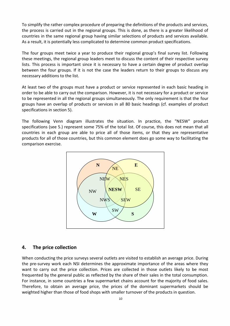
To simplify the rather complex procedure of preparing the definitions of the products and services, the process is carried out in the regional groups. This is done, as there is a greater likelihood of countries in the same regional group having similar selections of products and services available. As a result, it is potentially less complicated to determine common product specifications. The four groups meet twice a year to produce their regional group’s final survey list. Following these meetings, the regional group leaders meet to discuss the content of their respective survey lists. This process is important since it is necessary to have a certain degree of product overlap between the four groups. If it is not the case the leaders return to their groups to discuss any necessary additions to the list. At least two of the groups must have a product or service represented in each basic heading in order to be able to carry out the comparison. However, it is not necessary for a product or service to be represented in all the regional groups simultaneously. The only requirement is that the four groups have an overlap of products or services in all 80 basic headings (cf. examples of product specifications in section 5). The following Venn diagram illustrates the situation. In practice, the "NESW" product specifications (see 5.) represent some 75% of the total list. Of course, this does not mean that all countries in each group are able to price all of those items, or that they are representative products for all of those countries, but this common element does go some way to facilitating the comparison exercise.

4. The price collection

When conducting the price surveys several outlets are visited to establish an average price. During the pre-survey work each NSI determines the approximate importance of the areas where they want to carry out the price collection. Prices are collected in those outlets likely to be most frequented by the general public as reflected by the share of their sales in the total consumption. For instance, in some countries a few supermarket chains account for the majority of food sales. Therefore, to obtain an average price, the prices of the dominant supermarkets should be weighted higher than those of food shops with smaller turnover of the products in question.

NE

NESW

NEW

NWS

NW

S W

E N

SW

NES

SEW

SE

11

In most countries the outlets are selected by the NSI and a list of the selected shops is given to each price collector. If, for some reason the outlets cannot be selected by the NSI, the price collectors themselves will have to make the selection in the field. The selection must in such cases strictly adhere to the detailed instructions provided by the NSI. Such instructions should specify:

The type of outlet (department store. supermarket. market. etc)

The part of the city the outlet should be located (centre. off-centre. suburb)

The type of city area (residential. shopping. industrial)

The price/quality profile of shops.

5. Product specifications

The product specifications used in the European Comparison Programme (ECP) are either “brand and model specific” or “generic”. A “brand and model” specification designates the particular brand or model to be priced. A “generic” specification lists only the relevant technical parameters of the product to be priced; it does not identify any brand. A “brand and model” specification has a tight definition; countries pricing a specification stipulating a specific brand and model are, in principle, pricing identical products. A generic specification has a looser definition; countries pricing a generic specification are, in principle, pricing comparable products. It is of the higher importance that product specifications, particularly generic specifications, are sufficiently detailed to ensure that participating countries price products of the same quality.

Table 1: Examples of product specifications

Product Technical parameters

11.01.11.5 Spaghetti

Brand: Buitoni. Barilla. Panzani Made from: hard wheat (durum) With eggs: no Length: approximately 30 cm Cooking time: approximately 11 minutes Quantity: 500 g +/- 100 g Specify: brand(s) Reference quantity: 500 g

11.01.12.4 Chicken for roasting

Fresh or frozen: fresh Free range: yes With head and feet: no With heart. liver and gizzard: yes Weight: 1.1 kg +/- 0.1 kg Reference quantity: 1 kg

11.03.12.2 Women’s trousers

Brand: upper cluster of well-known brands Type: jeans Composition: 95% cotton and 5% elasthane Style: low waisted; straight leg. bootcut or flared; no tucks or pleats; with belt loops Colour: single Lining: no Fastener: buttons in front Pockets: three front pockets. two back pockets Finishing: well-finished button holes and seams Specify: brand(s) Reference quantity: one pair

11.04.32.1 Plumber

Service: replacement of two old taps by two new taps (one for hot water. the other for cold water) in a wash basin of a bathroom by a qualified worker; no changes to existing pipes required Time: during the working day Include: any travel cost charge. 30 minutes each way Exclude: cost of materials Specify: price for the complete service and travel costs Reference quantity: one service

12

Product Technical parameters

11.05.11.1 Kitchen chair

Brand: well-known brand Type: straight back chair. backrest with slats Made from: solid pine. lacquered Dimensions (H x W x D): approximately 90 x 45 x 40 cm With: struts Without: arms and upholstery Specify: brand or shop (see guidelines) Reference quantity: one chair

11.05.31.1 Cooker

Brand: lower cluster of well-known brands Energy source: gas Cooking surface: four burners with safety system Covering hood: yes Oven heating: conventional Grill in the oven: no Dimensions (H x W x D): 85 x 50-60 x 60 cm Pull-out system: conventional Easy to clean: no Timer: no Colour: white Specify: brand(s). model. parameters and energy efficiency if available Reference quantity: one cooker

6. Data processing

Whilst the control and verification of the end results for all the countries is important, the review process in Brussels is particularly important as a mistake in a Brussels price will affect all other countries participating in the Article 64 exercise through the miscalculation of bilateral parities.

After the data collection is completed by the NSIs they check their own results. This process is facilitated by standardised formatting and reporting software, which includes automated identification of "outlier" prices (individual price observations which exceed normal tolerance limits, defined in various ways). Countries are required to make an initial check of their own data against those of neighbouring/similar countries. In a subsequent stage, the data are reviewed within each group to minimise any inconsistencies. If there are results that seem to be very different for one country the group leader will request a verification or correction of the result. For the purpose of identifying unexpected price variations, suspicious-looking price levels and other inconsistencies, Quaranta Table analytical reporting software is used. This table provides the main diagnostic tool for the checking and approval of the survey results. It works by providing information about both the Basic Headings and the specific items in the Basic Headings. The examples of Quaranta Tables below are followed by a brief description of how to read them correctly. If the price is found to be wrong, due to for instance mistaken reference quantity or translation problems, different solutions are possible. It may be possible to "split" the product definition (eg. into two packet sizes) and redistribute prices accordingly, allowing better comparisons between countries. Alternatively, a country may have to delete individual price observations (especially where they are a particularly extreme outlier). Occasionally the country will have to delete the whole set of collected prices for a product definition (unless, in exceptional circumstances, it is able to undertake a new price survey for that particular item). Such deletion may not be problematic if there is an adequate number of prices for other item definitions, especially where

13

the product concerned is not representative for the country concerned (ie. no asterisk is attributed).

14

Table 2: An example of a Quaranta table

EUROSTAT- PPP: QUARANTA TABLES SURVEY: 2003-I Central group (final version) Date: 08.01.2004 Page: 1

[1] 11.01.11.1 Rice [2] Av. Weight: 59 [3] No. of it.: 8

[4] EKS method; Selected options: limits for XR-. PPP-indices = 80%. 125%. with *. without L/P limits [5] Var. Coef. (%): 19.7

[6] [7] XR

'NC/EURO'

[8] PPP

'NC/CUP'

[9] PLI (%) PPP/XR

[10] Weight/ 100000

[11] No. of Items

[12] Var. Coef.

[6] [7] XR

'NC/EURO'

[8] PPP

'NC/CUP'

[9] PLI (%) PPP/XR

[10] Weight/ 100000

[11] No. of Items

[12] Var. Coef.

OS 1.00000 1.01637 101.6 23.8 7: *4 13.8 LUX 1.00000 1.29062 129.1 74.0 6: *3 22.3

BE 1.00000 1.40005 140.0 34.6 8: *6 22.7 NL 1.00000 1.04821 104.8 40.6 7: *4 24.5

CH 1.54110 1.64876 107.0 58.3 5: *5 16.9 PL 4.35350 2.63721 60.6 47.5 5: *3 13.7

CZE 31.3910 18.9608 60.4 63.9 7: *4 25.7 SVK 41.0920 24.8722 60.5 149.5 7: *5 18.3

DE 1.00000 1.68260 168.3 13.8 7: *7 19.3 SVN 232.959 230.491 98.9 95.3 7: *3 13.4

HUN 245.180 199.895 81.5 91.1 7: *3 21.5 DE2 1.00000 1.61527 161.5 13.8 7: *7 16.3

1 [13] 11.01.11.1aa = CNS – Rice. long grain. 500 – 1000 g. specified brand. (reference quantity = 1000 g) [14] Var. Co.: 16.6

[15] [16] NC-price

[17]*

[18] Qts.

[19] Var. Co.

[20] Wn

[21] EURO-pr.

[22] EURO-In.

[23] Wn

[24] CUP-price

[25] CUP-In.

[26] Wn

[27] GM=> 2.74 [28] GM=> 2.64

OS 3.04 * 4 5.1 3.04 111 2.99 114

BE 3.01 * 13 16.8 3.01 110 2.15 82

CH 4.58 * 9 21.2 2.97 109 2.78 106

CZE 52.80 5 4.4 1.84 67 < 3.05 116

DE 3.18 * 12 14.2 3.18 116 1.89 72 <

HUN 533.20 5 8.6 2.17 79 < 2.67 102

LUX 3.46 * 5 9.1 3.46 126 > 2.68 102

NL 2.63 * 9 14.2 2.63 96 2.51 96

SVK 82.08 10 7.7 2.00 73 < 3.30 126 >

SVN 720.08 5 7.5 3.09 113 3.12 119

DE2 3.33 * 8 8.9 3.33 122 2.06 79 <

2 [13] 11.01.11.1ac = CN – Rice. long grain. 500 – 1000 g. well known brand. (reference quantity = 1000 g) [14] Var. Co.: 15.0

[15] [16]

NC-price [17]

* [18] Qts.

[19] Var. Co.

[20] Wn

[21] EURO-pr.

[22] EURO-In.

[23] Wn

[24] CUP-price

[25] CUP-In.

[26] Wn

[27] GM=> 1.69 [28] GM=> 1.71

OS 1.76 * 3 2.7 1.76 104 1.73 101

BE 2.75 * 9 12.4 2.75 162 > 1.96 115

CZE 24.53 * 4 14.6 0.78 46 < 1.29 76 <

DE 3.39 * 7 19.1 3.39 200 > 2.02 118

HUN 318.50 * 2 25.0 1.30 77 < 1.59 93

LUX 1.66 * 8 35.9 > 1.66 98 1.29 76 <

NL 1.86 5 30.1 1.86 110 1.77 104

PL 4.63 * 6 15.3 1.06 63 < 1.76 103

SVK 50.10 * 7 10.4 1.22 72 < 2.01 118

SVN 356.67 * 14 24.7 1.53 90 1.55 91

DE2 3.25 * 10 10.2 3.25 192 > 2.01 118

Note: In Germany, both the present capital, Berlin, and the former capital, Bonn. are surveyed. DE is Berlin and DE2 is Bonn. Their prices are validated separately and then combined as unweighted arithmetic means. The asterisks from Berlin determine representativity.

15

Table 2 : Reading the Quaranta Table

Basic heading table [1] The basic heading covered by the table.

[2] Av. Weight or average weight: The average expenditure weight for the group of countries covered by the Quaranta table. The unweighted arithmetic mean of the national weights in column [10]. Like the national weights it is scaled to 100.000.

[3] No. of It. or number of items: The number of products specified for the basic heading. The number of product tables comprising the Quaranta table.

[4] Identifies the options selected when preparing the Quaranta table – namely: the method used to calculate the PPPs for the basic heading PPPs in column [8]; and the range in which the EURO-indices in column [22] and the CUP-indices in column [25] should lie if they are not to be flagged as outliers in column [23] or column [26]. In this case, the EKS method, with representativity (*), without limits on the Paasche-Laspeyres spread, has been used to calculate the PPPs; and the range in which the EURO-indices and CUP-indices should lie is 80 to 125. Selected options can be changed as required.

[5] Var. Coef. or variation coefficient: The unweighted arithmetic mean of the variation coefficients of the products at [14]. The average variation of the standardised price ratios of the products priced for the basic heading.

[6] Abbreviated names of the countries covered by the Quaranta table.

[7] XR ‘NC/EURO’: The market exchange rates (XR) of the countries expressed as the number of units of national currency (NC) per euro. The exchange rate is 1.00000 for countries in the Euro area.

[8] PPP ‘NC/CUP’: The PPPs for the basic heading calculated as specified in [4] – that is, the EKS method - and expressed as the number of units of national currency (NC) per conventional unit for expressing parities (CUP). The CUP is obtained by first standardising the EKS PPPs and then multiplying them by a coefficient to scale them to the euro. The scaling coefficient is defined as the unweighted geometric mean of the NC/EURO exchange rates in column [7]. The prices used to calculate the PPPs are the average survey prices in national currencies that countries report for the products they priced for the basic heading – that is, the NC-prices in column [16].

[9] PLI (%) PPP/XR or price level indices. The PPPs in column [8] expressed as a percentage of the exchange rates in column [7].

[10] Weight/100000: National expenditure weights scaled to 100.000. That part of a country’s household individual consumption expenditure that is spent on the basic heading when both expenditures are expressed in national currency and valued at national price levels. Household individual consumption expenditure is defined by the domestic concept, before adjusting for net purchases abroad.

[11] No. of items: Number of products that are priced by each country and the number of products priced by each country that are representative – that is, the number of products assigned an asterisk (*).

[12] Var. Coef. or variation coefficient: The standard deviation expressed as a percentage of the arithmetic mean of the indices of PPP converted prices – that is, the CUP-indices in column [25] - for all products priced by the country irrespective of whether they are representative or unrepresentative. CUP-indices of products priced by only one country are not included.

Product table [13] Code, name and summary definition of the product covered in the subsequent product table.

[14] Var. Co. or variation coefficient: The standard deviation expressed as a percentage of the arithmetic mean of the indices of PPP converted prices for a product – that is, the CUP-indices in column [25].

[15] Abbreviated names of the countries pricing the product.

[16] NC-price: Average survey price in national currency (NC).

[17] Representativity indicator. Generally, representativity is marked by an asterisk (*), but in the case of rents numerical weights (percentages) are shown.

[18] Qts. or quotations: The number of price observations on which the average survey prices - the NC-prices - in column [16] are based.

[19] Var. Co. or variation coefficient: The standard deviation expressed as a percentage of the arithmetic mean of the price observations underlying the average survey price in column [16].

[20] Wn or warning: Variation coefficients in column [19] that have a value which is greater than the selected crucial value of 33 per cent are flagged by >.

[21] EURO-pr. or EURO-prices: The prices in national currency – the NC-prices – in column [16] converted to euros with the exchange rates in column [7].

[22] EURO-In. or EURO-indices: Indices based on the exchange rate converted prices – the EURO-prices – in column [21]. The EURO-prices expressed as a percentage of their geometric mean at [27]. Referred to in the text as “standardised price ratios based on exchange rate converted prices”.

[23] Wn or warning: Flags the indices of exchange rate converted prices – the EURO-indices – in column [22] that have a value which falls outside the selected range of 80 to 125 [4]. Values that are below 80 are flagged by <, values above 125 are flagged by >.

[24] CUP-price(s): The prices in national currency – the NC-prices – in column [16] converted to the conventional unit in which to express parities (CUP) with the PPPs in column [8].

[25] CUP-In. or CUP-indices: Indices based on the PPP converted prices – the CUP-prices – in column [24]. The CUP-prices expressed as a percentage of their geometric mean at [28]. Referred to in the text as “standardised price ratios based on PPP converted prices”.

[26] Wn or warning: Flags the indices of PPP converted prices – the CUP-indices – in column [25] that have a value which falls outside the selected range of 80 to 125 [4]. Values that are below 80 are flagged by <, values above 125 are flagged by >.

[27] GM or geometric mean of the exchange rate converted prices – the EURO-prices – in column [21]. The use of a geometric here and in [28] insures invariance with respect to choice of numeraire.

[28] GM or geometric mean of the PPP converted prices – the CUP-prices – in column [24]. It will be the same as [27] when all countries covered by the Quaranta table have priced the product.

16

7. Review of consumer price surveys for Art.64 purposes

As product price data is obtained from the European Comparison Programme, it is therefore already reviewed and validated by Member States and Group Leaders. As already indicated in Chapter II, this review and validation is an iterative process, initially conducted at country level, then multilaterally within a small geographical group of countries, then multilaterally within the whole group of countries. In a sense there is also a final validation stage following use of survey results for computation of overall parities at aggregate level.

For the non-capital duty stations specific arrangements are put in place to collect and process data in the same way.

With 28 EU Member States, 5 additional non capital city duty stations in these Member States, and a further 9 other countries for which Eurostat is responsible under the ECP (ie. 42 locations), and c.1000 product definitions in the two/three surveys conducted each year, a detailed additional review of prices and products for Art.64 purposes could be time-consuming. Nevertheless, there is a potential justification for an additional review for Art.64 purposes due to the important method differences between the ECP calculations and the Art.64 calculations.

(a) For the final ECP calculations, the prices used are national, annual averages. By contrast, Art.64 PPPs use 1st July prices, and Art.64 PPPs for staff use capital city prices (see Chapter VII). Currently the same PPPs are also used as an input into the calculation of correction coefficients for pensioners (see Chapter VIII). In practice, spatial adjustment factors are typically at or near 1.00 for most products for most countries.

(b) The PPPs computed at basic heading level and reported in the Quaranta Tables for the ECP are transitive EKS PPPs. They are initially computed as Laspeyres-type/Paasche-type indices (geometric mean of ratio of average prices just for representative products for base/home country, where representativity is identified by the attribution of asterisks). By contrast, Art.64 PPPs currently use all the average prices (i.e. no representativity distinction is made), and Art.64 PPPs are bilateral with Brussels, not multilateral (so additional information from indirect linkages is not taken into account).

(c) A more detailed basic heading structure is used for the ECP calculation process than the 80-position structure used for Art.64 purposes, which effectively changes the implicit weighting of product groups within the basic headings.

(d) The consumption expenditure weightings are another important difference between the ECP and Art.64 PPP calculations. EU officials can have quite different incomes and spending habits to the national average population (eg. to retain links with their country of origin).

These method differences could mean that the ECP automated checking process overlooks price ratios which may be problematic for A64 purposes.

In the past, the A64 team has only received average prices, often long after the survey has taken place. For this reason, it has now been agreed that a review for Art.64 purposes will be undertaken in parallel to the review for ECP purposes. This is happening with effect from survey E08-2.

17

8. Treatment of missing values

Aggregation from BH PPP to overall PPP is done using detailed expenditure weights (see Chapter VII). This process requires the matrix of BH PPP to be complete. If for a given country there are no average prices for any of the product definitions within a basic heading, for which one or more of the definitions were however priced in Brussels, then the PPP for that BH will have to be imputed.

A theoretically neat solution would be to require such imputation using PPP from the next COICOP level of aggregation (e.g. BH 02.1.2 "Wine" using Group 02.1 "Alcohol"). However, in practice not all the products from a COICOP group may be covered by the same consumer price survey. A pragmatic alternative is therefore to estimate the missing BH PPP using just the set of PPP for BH which are available from the survey. Strictly this should be done using Laspeyres and Paasche weighted average PPPs and calculating the Fisher geometric mean PPP. In practice, a simple geometric mean of the relevant PPP may be sufficiently accurate.

18

III – HEALTHCARE

1. Introduction

The healthcare component is long acknowledged to be comparison-resistant due to the different service delivery systems in Member States. EU officials are entitled to reimbursement of some or all of their expenditure under the Joint Sickness Insurance Scheme (typically 80% depending on the nature of the intervention but sometimes more and sometimes less). Nevertheless, the balance of the unreimbursed expenditure on prescription medical care plus any expenditure on non-prescription medical care, still represents on average around 1.9% of total consumption in Brussels and around 1.4% in other duty stations (source: expenditure weights used for July 2014 aggregation calculation).

The ECP consumer price survey on healthcare compiles full prices (market prices and/or subsidised prices + subsidy) for doctor and paramedical services, dentist services; therapeutical equipment; other medical products and a long list of pharmaceutics. In the ECP programme these are five separate basic headings: in the A64 calculations the data is combined into a single healthcare basic heading.

For ECP purposes, an input cost approach is applied to compare expenditures on hospital care (another basic heading). Until the July 2015 exercise this approach was not used for A64 purposes: hospital care was not taken into account at all. To the extent that the level of full market prices for hospital care is different when compared to Brussels than is the case for comparison of other medical goods and services to Brussels, there was consequently a potential bias.

With effect from the July 2015 exercise, following test calculations, a new approach was adopted and implemented by the ECP, and is now integrated for use in the A64 exercise.

2. The new ECP approach to establish output-based measure for hospital care

ECP documents 13/P2/07 "New methodology for hospital PPPs" and 14/P2/06 "Publication of hospital PPPs", DELSA/HEA/WD/HWP(2014) "Comparing hospital and health prices and volumes internationally" and IARIW/33/6A "Comparing hospital prices and volumes across countries: a new approach" describe recent developments in the European Comparison Programme regarding the calculation of PPPs for hospital care. The ECP team now publish an analytical category PPP for hospital services on the Eurostat free data website. This PPP is integrated for the calculation of global PPP with effect from reference year 2013.

The new approach is output based. A set of 28 model cases is defined, describing typical medical and surgical interventions in hospitals. These were selected for representativity of intervention types and percentage of expenditure. International Classification of Disease codes are used to ensure comparable clinical diagnoses and procedures. Only lengths of stay within 1.5 days of the national mean are included. The list has been refined during pilot phases of the project 2007-2012. Quasi prices are then compiled for these services. Input costs for component elements are built up to an overall amount. These then approximate closely to what market price might have been (what government/insurance purchaser would be prepared to pay and what hospital provider would be prepared to accept). Data is compiled from a defined sample of representative hospitals in each Member State (up to 100%). Routinely-collected administrative information is used for this purpose.

19

Analysis of pilot results showed that several countries exclude consumption of fixed capital from their input costs calculation. To account for these differences, 4.8% was added for 8 Member States (Bulgaria, Denmark, Germany, Ireland, Croatia, Latvia, Lithuania, Hungary) - the percentage estimate is derived from national accounts data. The analysis also showed that some countries include research and development costs in their calculation. To account for these differences, 1.3% was removed for 8 countries (Bulgaria, Denmark, Estonia, Spain, Malta, Netherlands, Portugal, Romania) – the percentage estimate was also derived from national accounts data. Similarly, some countries included training and education costs in their calculation, and 1.2% was removed for the same 8 countries plus Ireland – also on the basis of national accounts data.

For the 2015 and subsequent surveys, ECP work will be contracted to an external company with extensive experience in health cost comparisons. Additional model cases will be added for long-term care (chronic pulmonary disease, acute bronchitis, concussion, multiple sclerosis).

3. Integrating the new ECP data for A64 purposes

The chosen approach is to integrate the new PPP for hospital care as part of a weighted arithmetic average, by recalculating intermediate PPP for medical and paramedical services, dentist services, therapeutic equipment, other medical products and pharmaceutics (using price data from the most recent ECP survey on healthcare), and combining this with the new intermediate PPP for hospitals for the same year. The most recent detailed ECP breakdown of final household consumption expenditure is used as weights. The result is a single basic heading parity "Healthcare". This approach is used with effect from the July 2015 calculation.

20

IV – EDUCATION

1. Introduction

Education is long acknowledged to be a comparison-resistant component due to the different systems adopted in Member States for organising and delivering this service. Possible scenarios include:

Full payment by household at point of purchase, whether or not subsequently reimbursed by government or non-profit institution or private employer.

Part payment by household at point of purchase, with balance of price paid directly to the supplier by government or non-profit institution or private employer.

Full payment by government or non-profit institution or private employer at point of purchase. It is important that full-market prices in Brussels or a duty station are not compared directly with subsidised prices or free-at-point-of-delivery items in a duty station or Brussels.

Market prices for education can generally be identified in most Member States, although the degree to which they are representative of consumption will vary. In many Member States, Education is mainly a non-market service, with the majority of pupils and students receiving their education from non-market producers either free or at prices that are not economically significant. This makes Education comparison resistant because:

there are no prices with which to value output;

the units of output are more difficult to define and measure;

the differences in the quality of output between countries are less easily identified and quantified.

In this case, instead of compiling and comparing market prices for a defined item, the principal cost components have to be identified, and the aggregate compared:

Compensation of employees (wages, salaries and allowances that general government pays employees in selected occupations, such as teaching professionals, school administrators and support staff);

Intermediate consumption (supplies, including overheads);

Consumption of fixed capital. A problem with this approach is that the result does not reflect productivity differences.

2. Approach for the Article 64

Data was requested from PMO in 2011 and received in 2014. This consisted of information extracted from individual education declarations about schools attended by pupils of EU officials.

To complement this information, Eurostat collected additional data about costs in the European School system, costs in national systems (public schools), and prices in national systems (private schools).

21

Data sources for the calculations by School type:

On this basis, individual parities were established for European Schools (input costs), for state schools (quality adjusted input costs) and for private schools (output prices). A weighted average parity was then calculated using the pupil numbers as weights.

2.1 Cost data for European Schools

Costs for Type 1 European Schools are extracted from the Board of Governors central secretariat website. They are Category II fees, which are set equal to average cost per pupil (all cycles combined).

The value for Brussels is an average of the four schools (Woluwe, Uccle, Ixelles, Laeken). The cost data for European Schools in DE_Frankfurt, BE_Mol and LU_Luxembourg and LU_Mamer was not used as these are not duty stations for which CC are established. By contrast the data for ES_Alicante was included as this is the largest concentration of EU staff in Spain and there is no European School in Madrid. There are no Type 1 European Schools in most Member States.

The data for Type 2 and 3 "accredited" European Schools is not used, as although they offer the same curriculum leading to the same qualification, the delivery process is very different (notably use of locally-recruited staff rather than seconded teachers from national systems, and they operate under national law and funding).

2.2 Cost data for national non-fee paying schools

In the case of the non-fee paying schools, for each Member State the national annual average expenditure in EUR per pupil for primary and for secondary education level is provided by the Eurostat European Comparison Programme Team as a by-product from the annual ECP calculation exercise. This data is already quality adjusted for PISA outcomes. The detailed pupil numbers for primary and for secondary level (from PMO) are then used as weights to obtain an average cost (primary and secondary combined).

2.3 Price data for fee paying Schools

For the fee paying schools, the data received from PMO about schooling choices of EU officials is examined, as a guide for the selection of fee-paying schools located in duty station towns/cities. Price data from individual school websites in national currency is then compiled by members of the Eurostat Remuneration Team. An arithmetic average (weighted by pupil numbers) price for all schools in each duty station town/city is then computed.

22

Data is analysed separately for:

Anglophone international schools (e.g. COBIS, IB, American)

Other international schools (e.g. French AEFE, German ZfA)

Local private schools 2.4 Overall parity for Education

Parities for the European Schools are established by expressing the input cost data for each location relative to the cost for Brussels.

Parities for the national non-fee paying schools are established by expressing the input costs for each country relative to the cost for Belgium.

Parities for the fee paying schools are established by expressing the average price in national currency for each duty station relative to the average price for Brussels.

In order to derive an overall PPP for Education, a weighted arithmetic mean using pupil numbers is computed using (1) the input cost PPPs for European Schools and (2) the input cost PPPs for non-fee paying schools, and (3) the market price PPPs for fee paying schools.

Pupil numbers for Brussels are used to establish Laspeyres-type overall PPPs and those of duty station (inverse PPP) are used to establish Paasche-type PPPs. Finally, a Fisher-type PPP is then calculated as the geometric average (i.e. square root) of the Laspeyres and Paasche values.

3. Practical issue

There is no need for Member States to collect and submit data as use is made of information available from existing databases and a specific survey by Eurostat.

Due to the data collection workload on the Eurostat Remuneration Team, this survey and calculation is done on a three yearly cycle, with similar timing to the frequency of the ECP "Services" survey. In between these calculations, the updating of the Education basic heading parity will be done with the Education sub-index of the HICP10.

Apart from any change in costs/prices over time, under the proposed method a big change in pupil numbers in a given duty station (eg. due to staff mobility or pupil aging) may affect relative shares primary/secondary, and may therefore affect average cost/price. However, as such changes cannot easily be forecast and should occur without systematic bias towards one or the other category, and as the intention is not to measure evolution but to produce the best snapshot at each point in time, this approach is considered acceptable.

The focus is on education for school age children, not pre-school care or university studies, and not consumption of adult education and training services by EU officials themselves. However, as UoE statistics suggest that the majority of expenditures relate to standard schooling in primary/secondary cycles, this focus is considered acceptable.

10 The HICP sub-index is established using market prices for fee-paying schools.

23

V - ESTATE AGENCY RENT SURVEYS

1. General remarks

Correction coefficients are used to ensure equality of purchasing power of salaries of EU officials in the different duty stations. The rent paid for an apartment or house, due to its high weight in the total expenditure structure, plays a significant role in determining the overall correction coefficient. The rent parities are based on market rents obtained from special surveys of estate agencies. The scope of these surveys is to compare the average market rent for some specific kinds of dwellings in some pre-specified representative areas of Brussels with similar dwellings in similar (representative and comparable) areas in other EU capitals and duty stations. In practice it is very difficult to identify types of dwellings and districts of residence that are comparable to those selected for Brussels. The current methodology has arisen over many years of discussion and refinement.

Because of dwellings' uniqueness, housing cannot be dealt in such a precise way as other products, for which Eurostat draws up detailed specifications (often even with brand and model). However, Eurostat tries to obtain the best possible comparison, given the various constraints involved. The present method of calculating rent parities was introduced with effect from the 1990 quinquennial review of remuneration and is currently used for the annual reviews since 1991. It is mainly based on two elements:

an objective annual survey of estate agencies conducted jointly by Eurostat, the International Section on Remuneration and Prices (ISRP) of the Coordinated organisations11 and national statistical institutes (NSI) in each duty station, including Brussels. and

a moving average model representing the occupancy length over a six-year period. This chapter is concerned only with the rent surveys themselves. Chapter V deals with the moving average model.

2. The survey

In each place the survey is usually conducted the second quarter of the year (between end of March and end of June) by a team of normally 2 surveyors from the NSI (plus on observer either from Eurostat or ISRP12). The surveyors visit a certain number of experienced estate agents in order to obtain a good estimate of current rental values for pre-defined types of accommodation in some pre-selected neighbourhoods. At least ten agencies are visited in the larger cities, while in the smaller places it is possible to cover the market adequately with a smaller number. However six agencies are regarded as the absolute minimum. Agents are asked for current rents for dwellings in the middle-to-upper range of quality (i.e. above average but not luxury) and they are asked to give figures based on properties currently or very recently on offer.

11 The Co-ordinated Organisations are the NATO, the European Space Agency, the OECD, the Council of Europe, the Western European Union and the European Centre for Medium-range Weather Forecasts

12 Due to increase in number of duty stations over time, observers visit Member State on a rotational basis, with visits generally taking place every second year.

24

Overall average rents by type of dwelling are calculated aggregating all the agencies' results and discarding extreme values.

The quality of the rent parities depends on the quality of the rent surveys. Poor estimates of the rent levels will not lead to good parities even if highly sophisticated methods are applied. Close attention is therefore paid to the organisation and conduct of rent surveys. Here the NSIs play a vital role. The surveyors are provided with guidelines, which are revised by Eurostat and approved by the Article 64 Working Group.

The selection of dwelling types used in the survey is similar to the method used for all other products. A set of carefully specified dwelling types (currently 13) is established. All 13 are included in the Brussels survey, while in other places a selection is made which corresponds to locally representative dwelling types.

Table 6 shows the 13 possible specifications used at present and the kind of information collected in each place. So, for example, the 3-bedroom flats comparison between Paris and Brussels is based on the 110-130 m2 flats, while the 140-160 m2 flats are used to compare Athens to Brussels and the 80-100 m2 flats to compare London to Brussels.

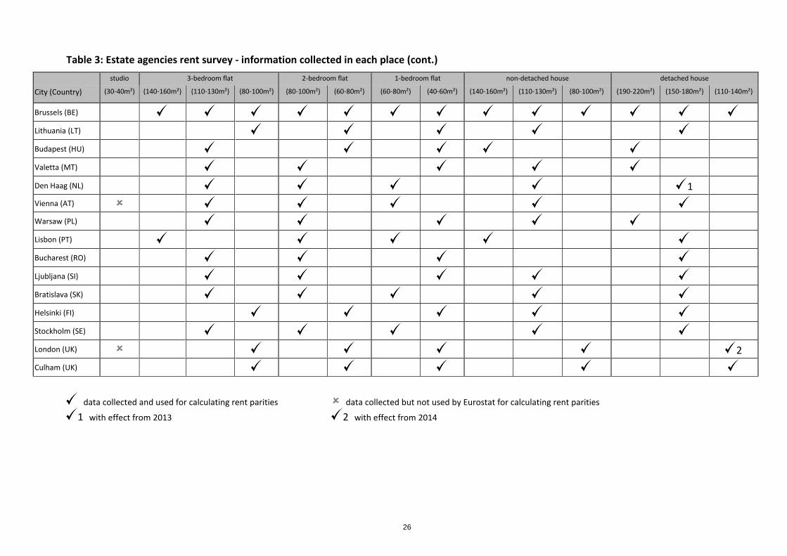
3. The questionnaire

A copy of the London questionnaire, as representative of all the other places is annexed (see appendix 2). The following instructions are included in the guidelines used by surveyors to fill the questionnaire (see appendix 3). Location: The areas are described as “good quality” residential areas favoured by expatriates and professional people such as civil servants, university staff, doctors, managers, etc. The quality should be good to very good, but not luxurious. Characteristics of accommodation: These are specified in the questionnaire. Living area includes cellars and attics if habitable. Accommodation types: At present there are a total of 6 broad categories of dwelling: Detached house Non-detached house (i.e. terraced or semi-detached) 3-bedroom flat 2-bedroom flat 1-bedroom flat Studio flat

Within each of these types, there are different sizes for total living space, depending on the styles commonly found in different places (e.g. UK and Ireland are generally smaller overall). The questionnaires are pre-printed with the sizes, which have already been established as being most commonly found in each place. In total there are 13 different combinations of dwelling type and size, but it is only in Brussels that all 13 are priced. In other places it is just one size-band for each dwelling type.

25

Table 3: Estate agencies rent survey - information collected in each place

studio 3-bedroom flat 2-bedroom flat 1-bedroom flat non-detached house detached house

(30-40m²) (140-160m²) (110-130m²) (80-100m²) (80-100m²) (60-80m²) (60-80m²) (40-60m²) (140-160m²) (110-130m²) (80-100m²) (190-220m²) (150-180m²) (110-140m²)

Brussels (BE)

Sofia (BG)

Prague (CZ)

Copenhagen (DK)

Berlin (DE)

Bonn (DE)

Karlsruhe (DE)

Munich (DE)

Tallinn (EE)

Dublin (IE)

Athens (EL) 1 1

Madrid (ES) 1 2

Paris (FR) 1 1

Zagreb (HR)

Rome (IT) 2

Varese (IT)

Nicosia (CY)

Riga (LV)

data collected and used for calculating rent parities data collected but not used by Eurostat for calculating rent parities

1 with effect from 2013 2 with effect from 2014

26

Table 3: Estate agencies rent survey - information collected in each place (cont.)

studio 3-bedroom flat 2-bedroom flat 1-bedroom flat non-detached house detached house

City (Country) (30-40m²) (140-160m²) (110-130m²) (80-100m²) (80-100m²) (60-80m²) (60-80m²) (40-60m²) (140-160m²) (110-130m²) (80-100m²) (190-220m²) (150-180m²) (110-140m²)

Brussels (BE)

Lithuania (LT)

Budapest (HU)

Valetta (MT)

Den Haag (NL)

1

Vienna (AT)

Warsaw (PL)

Lisbon (PT)

Bucharest (RO)

Ljubljana (SI)

Bratislava (SK)

Helsinki (FI)

Stockholm (SE)

London (UK)

2

Culham (UK)

data collected and used for calculating rent parities data collected but not used by Eurostat for calculating rent parities

1 with effect from 2013 2 with effect from 2014

27

Monthly rent: This is the actual rent currently payable for the various types of dwelling, whether payable partly in cash or not. Thus, if the asking rent normally has to be supplemented by separate cash payment (as happens in some places) it is the total rent that is considered. The figure excludes deposits, key money and similar one-off payments. Surveyors are instructed to ask for real rents (including any "under the counter" part). This can be particularly important in certain places.

Generally the information obtained for each of the specified dwelling types is a range of rentals within which most recent contracts have fallen (excluding the luxury end of the market). Sometimes agents prefer to give just an average value. It is clearly mentioned in the questionnaire, that accommodation rented by the employer must be excluded.

Charges made for general services (concierge. common cleaning. lighting of common parts. central heating. lift. etc.) are excluded as well as charges for gas, electricity, water etc., which are covered elsewhere in the correction coefficient calculation.

4. Management of the survey

a) Selection of appropriate districts

The selection criteria for the areas to be surveyed are of great importance. Dwellings and districts cannot be compared by physical characteristics alone as the duty stations vary enormously in both size and desirability. The rent survey covers those districts where professional people such as doctors, professors, lawyers, managers, etc., who pay the rents from their own pocket, actually live. Areas presently covered by the survey in Brussels as well in all other duty stations are reviewed and agreed bilaterally with respective NSIs before the start of each annual round of surveys to take into account the city-specific circumstances.

b) Quality of data: checking and controls

The main problems are extreme values (outliers) and the fact that the estate agent often has no difficulty in estimating the lower value of a range, but the upper value can be open-ended because there is hardly any limit to what can be charged for a dwelling of great luxury.

Eurostat tries to tackle this problem in the following way:

rent surveyors and local NSI representatives are responsible for the quality of data; they make effort to appreciate in the field whether extreme values are genuine cases or incorrect figures. They report their opinions to Eurostat.

on the basis of the surveyors' reports. Eurostat decides, case by case, whether extreme values are to be eliminated or not.

All the survey results and the surveyors’ reports are stored in Eurostat and analysed, taking also into account all the information contained in the surveyors’ reports. Before starting the process of the data (discussed in the next chapter), the NSI’s agreement to the final results is requested.

28

VI - STAFF HOUSING SURVEY AND THE HOUSING INDICES

The Staff Housing Survey (SHS) is carried out every 5 to 7 years in Brussels13 and the other duty stations. The survey's main purpose is to obtain the housing-type pattern (for the housing parities). Rents come from the Estate Agencies Surveys which are described in chapter III of this document. The questionnaire - sent to the EC staff in all the EU duty stations - asks for:

the type, the size in square metres and other characteristics of dwellings;

the monthly rent for the current and previous year. The rent ratios for each of the dwelling types are aggregated by using a housing weighting structure. Eurostat differentiates two different weighting structures:

a) Weights based on both tenants and owners

As the rent parity (basic heading 20) is also imputed to basic heading 21 (imputed rents of owner-occupiers) the housing-type weights should take into account both tenants and owners.

Table 4 shows how weights are calculated from the SHS for each duty station.

Table 4 Information from the Staff Housing Survey

TENANTS OWNER-OCCUPIERS TENANTS+OWNERS

Kind of dwelling Number Global expenditure

Number Global expenditure (Imputed rent)

Global expenditure (rents + imputed rents)

[1 [2 [3 [4 [5 [6

1 bedroom tn1 tx1 on1 ox1 = on1*tx1/tn1 tx1+ox1

2 bedrooms tn2 tx2 on2 ox2 = on2*tx2/tn2 tx2+ox2

3 bedrooms tn3 tx3 on3 ox3 = on3*tx3/tn3 tx3+ox3

detached houses tn4 tx4 on4 ox4 = on4*tx4/tn4 tx4+ox4

non-det. houses tn5 tx5 on5 ox5 = on5*tx5/tn5 tx5+ox5

TOTAL TN TX ON OX TX+OX

Number of tenants (tni) and owners (oni) by type of dwelling, as well as global expenditure of tenants by type of dwelling (txi) are available from the SHS. Imputed global expenditure of owners

by kind of dwelling (oxi) can be calculated as shown in column 5 and global expenditures for

tenants and owners is obtained in column 6.

13 Prior to 2013, survey was organised every year in Brussels as data was also used in calculation of the Brussels International Index measure used to monitor consumer price inflation, which is now replaced by Joint Brussels-Luxembourg Index.

29

Housing-type weights (wi) are the ratios between the global expenditure (tenants + owners) by kind of dwelling and the total expenditure:

wtx ox

TX OXi

i i

b) Weights based only on tenants or only on owners

There can be a relationship between certain characteristics of the reference population and the corresponding housing pattern. In particular there may be differences between patterns for “permanent” staff (officials staying for long periods in the duty station) and for “temporary” staff. The fact of staying permanently or temporarily in a place has at least two effects on housing-type patterns:

i) A small flat can be enough for a person working on the basis of a short posting, which may not involve the family and which may need just a minimum standard of comfort. By contrast, in duty stations where officials may stay for quite long periods, people tend to look for a permanent dwelling.

ii) In those places with a large number of permanent officials a high percentage are owners. The dwelling in this case is more frequently a house than a flat. Generally it is the case that for permanent and temporary staff there are different proportions of houses and flats. Moreover, owners tend to have bigger dwellings than tenants do.

For A64 purposes, a six year model is applied for rent parity calculation, reflecting the average duration of property occupation. In all duty stations, a weight pattern based on the dwelling choices of both tenants and owners is considered appropriate.

c) Imputed weights for places with insufficient information

There are places for which a correction coefficient has to be calculated, but too few officials are present to obtain specific housing-type weights. In such a case a European pool tenants’ pattern is applied. Before 2010 the European pool structures was based on tenants only. As of 2010 the structure is based on all occupants' pattern.

Table 5 shows an example of the 2012 calculation.

Table 5. SHS Calculation for 2012 exercise

SHS weights calculation

TENANTS+OWNERS

Kind of dwelling

Number Global

expenditure

Number Global

expenditure

(Imputed rent)

Global expenditure

(rents + imputed

rents) Tenants Total

1 bedroom 777 703,949 164 148,581 852,530 1 bedroom flat 23.05 8.96

2 bedrooms 1,053 1,228,393 827 964,749 2,193,142 2 bedroom flat 40.22 23.04

3 bedrooms 306 459,921 590 886,776 1,346,697 3+ bedroom flat 15.06 14.15

detached houses 139 242,235 1,127 1,964,020 2,206,255 Detached house 7.93 23.18

non-det. houses 242 419,543 1,443 2,501,655 2,921,198 Non-detached house 13.74 30.69

TOTAL 2,517 3,054,041 4,151 6,465,782 9,519,823 Σ 100 100

TENANTS OWNER-OCCUPIERS

Dwelling weights

BE-Brussels - 2012

30

A copy of the questionnaire used in the Brussels SHS is annexed (see appendix 6) together with guideline instructions for completion (see appendix 7). Participation in the survey is not compulsory.

31

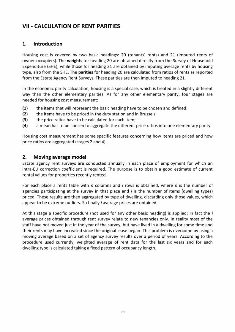
VII - CALCULATION OF RENT PARITIES

1. Introduction

Housing cost is covered by two basic headings: 20 (tenants’ rents) and 21 (imputed rents of owner-occupiers). The weights for heading 20 are obtained directly from the Survey of Household Expenditure (SHE), while those for heading 21 are obtained by imputing average rents by housing type, also from the SHE. The parities for heading 20 are calculated from ratios of rents as reported from the Estate Agency Rent Surveys. These parities are then imputed to heading 21.

In the economic parity calculation, housing is a special case, which is treated in a slightly different way than the other elementary parities. As for any other elementary parity, four stages are needed for housing cost measurement:

(1) the items that will represent the basic heading have to be chosen and defined; (2) the items have to be priced in the duty station and in Brussels; (3) the price ratios have to be calculated for each item; (4) a mean has to be chosen to aggregate the different price ratios into one elementary parity.

Housing cost measurement has some specific features concerning how items are priced and how price ratios are aggregated (stages 2 and 4).

2. Moving average model Estate agency rent surveys are conducted annually in each place of employment for which an intra-EU correction coefficient is required. The purpose is to obtain a good estimate of current rental values for properties recently rented.

For each place a rents table with n columns and i rows is obtained, where n is the number of agencies participating at the survey in that place and i is the number of items (dwelling types) priced. These results are then aggregated by type of dwelling, discarding only those values, which appear to be extreme outliers. So finally i average prices are obtained.

At this stage a specific procedure (not used for any other basic heading) is applied: In fact the i average prices obtained through rent survey relate to new tenancies only. In reality most of the staff have not moved just in the year of the survey, but have lived in a dwelling for some time and their rents may have increased since the original lease began. This problem is overcome by using a moving average based on a set of agency survey results over a period of years. According to the procedure used currently, weighted average of rent data for the last six years and for each dwelling type is calculated taking a fixed pattern of occupancy length.

32

Table 6 shows the weights used in the six years moving average model. These weights were derived from the results of the annual Staff Housing Survey (SHS) in Brussels and in the other main duty stations. It shows that the current year has a weight of 25% and the two most recent years a combined weight of 48%.

Table 6 Weights used in the six-year model

Year Current (t) t-1 t-2 t-3 t-4 t-5

Weight (%) 25 23 17 13 12 10

Before calculating the moving averages, all rent data used in the model is updated to the current year using the most appropriate price index. The index which is usually considered in a lease contract for updating rents is taken for this purpose. They are provided by the NSIs. The indices currently used are shown in table 7.

Table 7: Indices for updating rents

Country Place Index

BE Brussels Séries Indice santé/Gezondheidsindex

CZ Prague CPI

DK Copenhagen

Index of net retail price

DE Berlin COICOP 4.1+4.4 Bonn COICOP 4.1+4.4 Karlsruhe COICOP 4.1+4.4 Munich COICOP 4.1+4.4

EE Tallinn CPI

IE Dublin Sub-index rents from CPI

EL Athens CPI

ES Madrid CPI

FR Paris Séries coût de la construction

HR Zagreb CPI

IT Rome CPI - famiglie di operai e impiegati esclusi tabacchi Varese CPI - famiglie di operai e impiegati esclusi tabacchi

CY Nicosia CPI

LV Riga CPI

LT Vilnius CPI

HU Budapest CPI

MT Valletta CPI

NL The Hague CPI

AT Vienna CPI

PL Warsaw CPI

PT Lisbon CPI

SI Ljubljana CPI

SK Bratislava CPI

FI Helsinki CPI

SE Stockholm CPI

UK London CPI sub-index for private renters Culham CPI sub-index for private renters

33

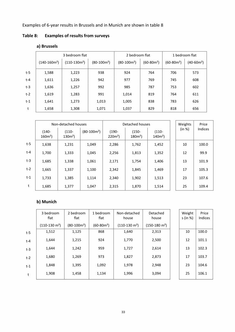
Examples of 6-year results in Brussels and in Munich are shown in table 8

Table 8: Examples of results from surveys

a) Brussels

3 bedroom flat 2 bedroom flat 1 bedroom flat

(140-160m²) (110-130m²) (80-100m²) (80-100m²) (60-80m²) (60-80m²) (40-60m²)

t-5 1,588 1,223 938 924 764 706 573

t-4 1,611 1,226 942 977 769 745 608

t-3 1,636 1,257 992 985 787 753 602

t-2 1,619 1,283 991 1,014 819 764 611

t-1 1,641 1,273 1,013 1,005 838 783 626

t 1,658 1,308 1,071 1,037 829 818 656

Non-detached houses Detached houses Weights (in %)

Price Indices

(140-160m²)

(110-130m²)

(80-100m²) (190-220m²)

(150-180m²)

(110-140m²)

t-5 1,638 1,231 1,049 2,286 1,762 1,452 10 100.0

t-4 1,700 1,333 1,045 2,256 1,813 1,352 12 99.9

t-3 1,685 1,338 1,061 2,171 1,754 1,406 13 101.9

t-2 1,665 1,337 1,100 2,342 1,845 1,469 17 105.3

t-1 1,733 1,385 1,114 2,340 1,902 1,513 23 107.6

t 1,685 1,377 1,047 2,315 1,870 1,514 25 109.4

b) Munich

3 bedroom flat

2 bedroom flat

1 bedroom flat

Non-detached house

Detached house

Weights (in %)

Price Indices

(110-130 m²) (80-100m²) (60-80m²) (110-130 m²) (150-180 m²)

t-5 1,512 1,125 868 1,640 2,313 10 100.0

t-4 1,644 1,215 924 1,770 2,500 12 101.1

t-3 1,644 1,242 959 1,727 2,614 13 102.3

t-2 1,680 1,269 973 1,827 2,873 17 103.7

t-1 1,848 1,395 1,092 1,978 2,948 23 104.6

t 1,908 1,458 1,134 1,996 3,094 25 106.1

34

The price indices in table 8 are used to update the rent data to the price level of the year t. The resulting rent data are presented in Table 9. The last row of table 9 (average rents) is obtained as a weighted average of the figures in each column, where the weights are those in table 8b. Thus, for example, a typical contemporary rent of a detached house in Munich in year (t-5) (2,420 EUR) would have risen by the year t to 2,568 EUR using the ratio of the price indices 106.1/100.0.

Table 9: Updated rents from table 8b (Munich)

3 bedroom flat

2 bedroom flat

1 bedroom flat

Non-detached house

Detached house

(110-130 m²) (80-100m²) (60-80m²) (110-130 m²) (150-180 m²)

t-5 1,582 1,177 908 1,716 2,420

t-4 1,702 1,258 957 1,833 2,588

t-3 1,681 1,270 981 1,766 2,673

t-2 1,696 1,281 982 1,844 2,900

t-1 1,848 1,395 1,092 1,978 2,948

t 1,908 1,458 1,134 1,996 3,094

Average rents 1,695 1,272 983 1,824 2,713

3. Rent ratios

The average adjusted rents for each of the i dwelling types are divided by the corresponding data for Brussels, giving i rent ratios.

An example of how rent ratios are calculated (in the case of Munich) is shown in table 10.

Table 10: Rent ratios for Munich

3 bedroom flat 2 bedroom flat 1 bedroom flat Non-detached house

Detached house

(110-130 m²) (80-100m²) (60-80m²) (110-130 m²) (150-180 m²)

Munich Average rents

1,695 1,272 983 1,824 2,713

Brussels Average rents

1,307 1,026 783 1,385 1,908

Rent ratios 1.2968630 1.2397660 1.255427 1.3169675 1.4219077

35

4 Aggregation of rent ratios

The rent ratios for each of the dwelling types are aggregated by using a housing weighting structure. See details in Chapter IV.

Various formulae have been developed to aggregate price ratios in order to measure the change between two situations (Brussels and a place x). The most common of these are the Laspeyres, Paasche and Fisher indices. These indices do not differ very much as long as the weights do not differ significantly.

Eurostat, in line with many other organisations, uses the Fisher index, which is the geometric average of the Laspeyres and Paasche indices.

(a) Laspeyres is the weighted arithmetic average of the rent ratios, using the weightings of the base period (0):

I

p

pw

wL

i

i

i

i

i

i

1

0

0

1

11

0

1

11

(b) Paasche is the weighted harmonic average of the inverse of the rent ratios, using the weights of the later period (1):

Iw

p

pw

P

i

i

i

i

i

i

1

1

11

0

1

1

1

11

(c) Fisher is the geometric average of the Laspeyres and Paasche indices:

I I IF L P

An example of rent parity calculation is shown in table 11.

36

Table 11: rent parity for Munich

3 bedroom flat

2 bedroom flat

1 bedroom flat

Non-detached house

Detached house

Totals

(110-130 m²) (80-100m²) (60-80m²) (110-130 m²) (150-180 m²)

Munich Average rents 1,695 1,272 983 1,824 2,713

Weights 17.80 17.10 7.80 32.10 25.20 100

Brussels Average rents 1,307 1,026 783 1,385 1,908

Weights 13.06 23.53 10.64 30.24 22.53 100

Price ratios 1.29720 1.23960 1.25498 1.31743 1.42145

Laspeyres index = 1.3706 (using Brussels weights)

Paasche index = 1.3759 (using duty station weights)

Fisher index = 1.373

5. Checks and analyses

As shown in previous paragraphs, several variables influence the final result of the rent parity. The rent parities for the year t are affected by the following factors:

introduction of rent data for the year t.

deletion of the rent data for t-6 from the 6-year moving average model

price indices used for updating the rents for (t-5) to (t-1) to the price level of year t. and

new dwelling-type weights based on staff housing surveys. All these effects as well as the total change in rent parities are shown in table 12.

37

Table 12: Change in rent parities from 2012 to 2013 - decomposition of effects (in %)

Places of employment

Deletion of survey

Introduction of survey

Price index Dwelling structure

Total change

2007 2013 2013

BG Sofia -11.6 -0.5 0.8 0.0 -11.4

CZ Prague -4.9 -0.6 -0.1 0.0 -5.5

DK Copenhagen 0.8 -1.5 -0.6 0.0 -1.2

DE Berlin 2.1 -0.2 -0.2 0.0 1.6

Bonn 1.2 0.3 -0.2 0.0 1.3

Karlsruhe 1.5 0.6 -0.2 0.0 1.9

Munich 4.0 0.6 -0.3 0.0 4.3

EE Tallinn -3.2 -1.5 1.5 0.0 -3.2

EL Athens -5.9 -2.6 24.2 0.0 13.8

ES Madrid -3.9 -1.2 -9.5 0.0 -14.1

FR Paris 0.6 -0.4 20.1 0.0 20.4

HR Zagreb 0.5 -1.3 12.8 0.0 11.9

IE Dublin 1.2 1.6 3.3 0.0 6.2

IT Rome -4.9 -1.5 -0.3 0.0 -6.6

Varese -2.4 -0.5 -0.3 0.0 -3.2

CY Nicosia -2.7 -1.4 -1.2 0.0 -5.2

LV Riga -2.2 -0.6 -1.2 0.0 -4.0

LT Vilnius -8.2 1.8 -0.3 0.0 -6.9

HU Budapest -4.2 -1.1 0.2 0.0 -5.1

MT Valletta -1.9 1.0 -0.1 0.0 -1.0

NL The Hague -1.8 -0.3 8.1 0.0 5.9

AT Vienna -1.3 1.4 0.3 0.0 0.4

PL Warsaw -4.1 -0.6 -0.8 0.0 -5.4

PT Lisbon -3.9 0.2 -0.5 0.0 -4.2

RO Bucharest -8.8 -1.8 3.0 0.0 -7.8

SI Ljubljana -5.0 -1.1 0.2 0.0 -5.9

SK Bratislava -1.5 -0.7 -0.1 0.0 -2.3

FI Helsinki 0.6 -0.4 -0.2 0.0 0.0

SE Stockholm 2.2 1.0 -1.4 0.0 1.8

UK London 2.0 0.6 -0.4 0.0 2.2

Culham 1.3 0.9 -0.4 0.0 1.8

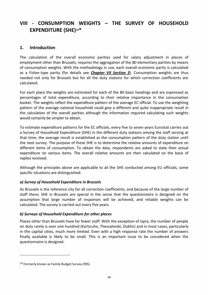
38

VIII - CONSUMPTION WEIGHTS – THE SURVEY OF HOUSEHOLD EXPENDITURE (SHE)14*

1. Introduction

The calculation of the overall economic parities used for salary adjustment in places of employment other than Brussels, requires the aggregation of the 80 elementary parities by means of consumption weights. With the methodology in use, each overall economic parity is calculated as a Fisher-type parity (for details see Chapter VII Section 3). Consumption weights are thus needed not only for Brussels but for all the duty stations for which correction coefficients are calculated.

For each place the weights are estimated for each of the 80 basic headings and are expressed as percentages of total expenditure, according to their relative importance in the consumption basket. The weights reflect the expenditure pattern of the average EC official. To use the weighting pattern of the average national household could give a different and quite inappropriate result in the calculation of the overall parities although the information required calculating such weights would certainly be simpler to obtain.

To estimate expenditure patterns for the EC officials, every five to seven years Eurostat carries out a Survey of Household Expenditure (SHE) in the different duty stations among the staff serving at that time; the average result is established as the consumption pattern of the duty station until the next survey. The purpose of these SHE is to determine the relative amounts of expenditure on different items of consumption. To obtain the data, respondents are asked to state their actual expenditure on various items. The overall relative amounts are then calculated on the basis of replies received.

Although the principles above are applicable to all the SHE conducted among EU officials, some specific situations are distinguished:

a) Survey of Household Expenditure in Brussels

As Brussels is the reference city for all correction coefficients, and because of the large number of staff there, SHE in Brussels are special in the sense that the questionnaire is designed on the assumption that large number of responses will be achieved, and reliable weights can be calculated. The survey is carried out every five years.

b) Surveys of Household Expenditure for other places

Places other than Brussels have far fewer staff. With the exception of Ispra, the number of people on duty rarely is over one hundred (Karlsruhe, Thessaloniki, Dublin) and in most cases, particularly in the capital cities, much more limited. Even with a high response rate the number of answers finally available is likely to be small. This is an important issue to be considered when the questionnaire is designed.

14 Formerly known as Family Budget Survey (FBS)

39

In extreme cases, like places with few officials (i.e.: capital cities) the reduced sample does not permit to estimate reliable consumption weights and a common structure, pooling all the questionnaires from these places, is derived.

2. The SHE in Brussels

a) Main features of the Brussels questionnaire

The questionnaire is divided into five parts:

Part 1 Personal information

Consists of some general information about the status, household composition and accommodation. The information given in this section is essential to validate the survey results and to extend these to the total population of EU officials in Brussels.

Part 2 Dwelling related regular bills in the country

This section concerns the main regular bills such as telephone, electricity, water, local and housing taxes, etc. The usual, or average, amount which is currently paid, together with the frequency, is shown in this section.

Part 3 Daily expenses of the household in the country (14 day diary)

This section records day by day during 2 consecutive weeks, all expenditure on food and food-related articles - such as restaurants and staff canteens.

Part 4 Yearly or average monthly expenses

This is a section in which items not already included in the previous parts are recorded. Total expenditure during a 12-month period in those items is recorded. In case of small or frequent expenditures (e.g. newspapers. flowers. cinema tickets) a monthly average instead of a total can be given. In the case of cars, purchases and sales during the last 5 years are requested.

Part 5 Education and health

This section concerns expenditures and reimbursements for education and health care in the last 12 months.

In accordance with the specific methodology approved for EU purposes, the focus is solely on expenditure in the duty station itself and information collected about out-of-area expenses plays no role in the calculation process15.

The design and content of the questionnaire has been refined over time to minimise the response burden and maximise the quality of the information collected. In general, there is only one question relating to each BH, although there are some exceptions to this rule (e.g. insurances). The 2009 survey was organised simultaneously as a traditional paper survey, an Excel file and a web-based questionnaire.

15 This is a difference from the approach taken by the United Nations.

40

See in appendix 4a the model used in the 2009 Brussels survey (and the glossary in appendix 5).

b) The method to impute rents for owner occupied dwellings

The method followed to impute rents declared in the Brussels SHE to owner-occupiers is to associate the average rents of each dwelling class to all owner-occupiers of the same dwelling class. This procedure is in line with the Commission Decision of 18.7.1995 (JO L186. 5.8.1995) on imputed rents estimation, recommending the use of stratification characteristics closely connected with housing and based on real rents.

The SHE questionnaire records the following variables connected with housing:

Type of dwelling (detached house, semi- or non-detached house, flat); Number of bedrooms;

Total area of living space. Given the sample size constraints, not all the possible classes are used but only those likely to have significantly different average rents. The following classes are defined:

1 Studio 2 Apartment 1 bedroom, <60 m2 3 Apartment 1 bedroom, >60 m2 4 Apartment 2 bedroom, <80 m2 5 Apartment 2 bedroom, >80 m2 6 Apartment >2 bedroom, <120 m2 7 Apartment >2 bedroom, >120 m2 8 House terraced or semi-detached <140 m2 9 House terraced or semi-detached >=140 m2 10 House detached <190 m2 11 House detached >=190 m2

3. SHE for places of employment other than Brussels

a) Preliminary remarks

For places other than Brussels different considerations apply. In the places where there are large centres (e.g. Ispra, Dublin, Thessaloniki, etc.) there exists the possibility of obtaining reasonably large numbers of SHE respondents - though not on the same scale as in Brussels. In some places the combined number of officials (including staff of EU institutions and EU agencies, personnel of the European Schools, the Co-ordinated Organisations, EuroControl, European Patent Office, etc.) – either in a single duty station or combining several places of employment within the same country - is large enough to provide a reasonably reliable estimate of average consumption patterns.

However in those places (mainly capital cities) where there are relatively few officials, there are problems in obtaining enough completed SHE questionnaires to be statistically viable, even if a 100% response were obtained (estimates from small samples will not necessarily represent the target average).

41

The two cases mentioned above need to be treated differently when estimating consumption weights.

Particular problems in the estimation of consumption weights exist for those countries with more than one place of employment and where a separate correction coefficient is applied.

All these issues are treated in detail in the following sections.

b) SHE in places with sufficient staff population to estimate reliable weights.

For these places, basically those with a sufficiently large combined population - either in a single duty station or combining several places of employment within the same country (staff of EU institutions and EU agencies, personnel of the European Schools, the Co-ordinated Organisations, EuroControl, European Patent Office etc.) a questionnaire similar to the one for Brussels is used. The principal difference is the "personal information" part, which is simplified. The questionnaire was reviewed in 2010 in collaboration with the United Nations International Civil Service Commission and the then Inter-Organisation Section of the Co-ordinated Organisations. See in appendix 4b the model used in the 2013 surveys.

c) Consumption weights for places with few officials

Until 2009:

The method recently applied to estimate consumption weights for places with few officials was approved by the Article 64 Working Party in February 1995 and is based on the average of weighting patterns from all places, except Brussels, as they are considered to have similar characteristics. This method treats housing separately from other items of expenditure.

Considering non-housing items list, the method starts from the fact that no basis exists for calculating detailed weights specific to each place: there is no possibility of a special FBS amongst international staff, and the national weights are not relevant. A proxy is therefore sought. Available SHE data show that there is a reasonable degree of similarity amongst the consumption patterns of international officials (at least at a high level of aggregation) regardless of their place of employment. Therefore, a set of average weights at the level of 12 main consumption groups is calculated. These weights are then disaggregated down to the 80-heading level, excluding housing, using national weighting patterns.

Housing weights are calculated based on the Brussels weight, corrected by the housing correction coefficient for each duty station. After introduction of the housing weights, the 80 basic headings are re-scaled to 1000.

The places used for the average weighting are those where SHE have been conducted - a sort of European pool excluding Brussels (given that Brussels represents more than 75% of the total population, its inclusion would dominate a weighted average supposed to reflect the numbers of officials in each place of employment). Furthermore since the purpose of the exercise is to construct a proxy for a Paasche-type “local” weighting, it would have not been logical to include Brussels as, of course, the Laspeyres part of the final Fisher index is wholly Brussels based. Thus the solution retained is to calculate an average set of weights based only on SHE responses from places other than Brussels.

42

From 2009:

A regional weighting structure is constructed, grouping survey responses together for "low-number-of-staff duty stations" within the socio-politico-economic-geographic groups of the European Comparison Programme. These 'pool' weights are then adjusted for each country by correcting housing expenditure using the rent correction coefficient, and re-scaling to 1000.

Under the memorandum of understanding signed with the United Nations and the Coordinated Organisations, it is sometimes possible to combine results for expatriate staff.

d) Consumption weights for countries with more than one place of employment

The estimation of consumption weights, although based where possible on local SHE, presents particular problems for those countries with more than one place of employment and where a separate correction coefficient is applied: Germany, Italy and the UK. Current practices differ according to the country taking into account the size of the population and the response rate to the survey. At present the situation is:

In the UK the same weighting pattern is used for Culham and London (i.e. the structure established for London is also applied for Culham).

In Germany, the same weighting pattern is generally used in all four places of employment (Berlin, Bonn, Karlsruhe and Munich*), pooling survey responses together with replies from other places in Germany (eg. Frankfurt, Köln). However, if there are sufficient replies to justify individual weighting structure for the large staff concentrations in Karlsruhe and in Munich, these could be used.

In Italy, Ispra (Varese) has its own survey-based weighting pattern, while Rome has a separate one based on completed questionnaires from Rome and other places in Italy (eg. Milan/Parma/Turin).

There are a number of other countries, where there are multiple duty stations, but no separate correction coefficient. For these countries, responses from all locations in the country are aggregated, for example:

Belgium (Brussels*/Mol);

Ireland (Dublin/Grange/Cork);

Greece (Athens/Thessalonika/Heraklion);

Spain (Madrid/Alicante/Barcelona/Bilbao/Sevilla/Vigo);

France (Paris*/Angers/Bretigny*/Cadarache/Lille/Marseille/Strasbourg*);

Netherlands (Amsterdam/TheHague*/Bergen/Maastricht*/Noodwijk*/Petten);

Portugal (Lisbon/Porto);

UK (London/Belfast/Bramshill/Cardiff/Culham/Edinburgh/Reading*).

* indicates a high concentration of staff for a partner organisation.

e) Processing family budget survey responses

The majority of responses from surveys amongst active officials are obtained via an online survey questionnaire tool, but a small number of paper questionnaires are also received and manually

43

coded into similar format for subsequent processing. By contrast the majority of responses to periodic survey amongst retired officials are received in paper (or PDF) format.

Expenditure responses are first converted from quinquennial/annual/monthly/weekly/daily format into a common (annual) basis. Information is then reviewed using automatic algorithms and manual checks for reasonableness and completeness. Where possible gaps are filled by imputation.

Analysis includes comparison of results with recent weighting structures from other sources (eg. national Consumer Price Index, national Household Budget Survey, EU staff housing survey, similar survey amongst United Nations personnel).

44

IX - CORRECTION COEFFICIENTS FOR OFFICIALS

1. Introduction

The basic principle behind the application of correction coefficients is that when officials are serving in posts outside Brussels and Luxembourg, they should not have to suffer financially because of higher living costs in their duty station. Equally, if the cost of living at a particular duty station is lower than in Brussels and Luxembourg, officials should not gain an unfair advantage over their counterparts in Brussels and Luxembourg. For this reason, salary adjustment of EU officials outside Brussels and Luxembourg requires to compare relative living costs between Brussels and Luxembourg and the places where these officials are on duty. The technique is to compare the price of a “basket” of goods and services purchased by the average EC official in Brussels with the price of the same basket in each of the other places of employment.

The full range of goods and services, which comprise the total expenditure of an average EC official is divided into 80 groups, called “Basic Headings” (such as footwear, local public transport, bread and cereals, tobacco etc.). Within these “Basic Headings”, the products are selected and specified in enough detail to allow prices in a reasonably narrow range to be collected. The choice of products is agreed at regular meetings between national statistical institutes (NSI) under the supervision of Eurostat. The potential list is endless, but the selection made must be reasonably small for practical purposes. The overall list contains more than 3000 items. Between each duty station and Brussels a parity is obtained for each of the 80 “Basic Headings”. Each elementary parity is calculated as the geometric mean of the price ratios for the items within the basic heading, which have been priced in Brussels and in the duty station. In order to calculate these elementary parities, prices of as many as possible of the items are collected by NSIs in each duty-station through special surveys carried out periodically (see chapter II). Several price quotations for each item are obtained and averaged. The calculation of a global economic parity requires the aggregation of the 80 elementary parities using consumption weights (see chapter VI). Each overall economic parity is calculated as a Fisher parity (geometric mean of Laspeyres and Paasche parities). Thus average prices and consumption weights are needed not only for Brussels but also for all the duty stations for which salaries are adjusted (for details see the following sections).

2. From price surveys to elementary parities

Chapter II gives a detailed description of all activities concerning price surveys. The overall list of products and services priced contains about 3000 items. The items are classified according to the classification system COICOP. COICOP (Classification of Individual COnsumption by Purpose) has been adopted as a national accounts classification for consumer expenditure applying to all national accounts as from 1999. It also applies for the Harmonised Indices of Consumer Prices (HICP).

45

According to COICOP, all products and services are first broken down into 12 main groups:

(1) Food, and non-alcoholic beverages (2) Alcoholic beverages and tobacco (3) Clothing and footwear (4) Housing, water, electricity, gas and other fuels (5) Furnishings, household equipment and maintenance of house (6) Health (7) Transport (8) Communication (9) Recreation and culture (10) Education (11) Hotels. cafes and restaurants (12) Miscellaneous goods and services

Each of the 12 groups is then broken down into sub-groups, which in turn are further broken down into more detailed groups. This operation continues until the most detailed level of the classification for which elementary parities are calculated. This level refers to as so called "basic heading". An exhaustive classification for the correction coefficients calculation comprises 80 basic headings (see appendix 1). The basic headings have a dual role:

first of all, they constitute the most detailed level for which realistic expenditure data (weights) can be obtained by the Surveys of Household Expenditure regularly conducted among the staff serving in the different EU duty stations (see chapter VI).

secondly, they match reasonably homogeneous groups of products from which a number of products are selected for price surveys (see chapter II).

As mentioned above, average prices for each product and place are calculated at the time of the survey. Price ratios between the duty station and Brussels for each product are then calculated. The geometric mean of these price ratios for the products belonging to the same basic heading is called elementary parity. So, there are in total 80 elementary parities for each duty stations reflecting the relative price levels in these duty stations comparing to those in Brussels.

Once a new price survey is conducted and the elementary parities for the basic headings concerned are calculated, they replace the existing elementary parities (derived from the previous survey and updated using harmonised price indices – HICP, see section 4). All elementary parities are then updated to the month of June of the current year for the purpose of annual review (to December, for the purpose of intermediate review).

The 80 elementary parities are then aggregated to one global parity using the consumption weights derived from the Survey of Household Expenditure (see chapter VI).

46

3. Calculation of the global parity

Using the 80 basic parities and the specific weights the overall parity is calculated in two ways: the first uses the consumption pattern for the reference city (Brussels) (this is a type of Laspeyres index); the second uses the consumption pattern for the duty station (this is a type of Paasche index). In accordance with standard practice for international comparisons both types of index are calculated and the geometric mean of the results (a Fisher index) is the one actually used.

First step is the calculation of the basic parities, which are obtained as geometric means of the price ratios for all the common items between place X and Brussels:

where: j = Basic heading 1 to 80

i = Item i

k = Number of items priced both in Brussels and in place X

PiX = Average price of item i in place X

PiB = Average price of item i in Brussels

A first possible aggregation of these basic parities can be obtained using the Brussels pattern of consumption in the following formula:

80 1

80 1

j Bj

j Bj j L B X

W

W PPA PPA

where: PPAj = Basic parity j for place X

WBj = Weight of heading j in the Brussels consumption structure

L = Laspeyres type index

Another aggregation can be obtained using place X consumption structure:

80 1

80 1

1 j Xj

j

j Xj P B X

W PPA

W PPA

where: WXj = Weight of heading j in the place X consumption structure

P = Paasche type index

k

k

i

iB

iXj

BX

P

PPPA 1

k i

47

The geometric mean of the two aggregated indices gives a Fisher type overall parity:

Derivation of the correction coefficient

Finally, for the non-Euro zone countries it is necessary to take the ratio between the Fisher overall parity and the exchange rate between Euro and the national currency for calculating the Correction coefficient.

where: TX/B = Remuneration exchange rate, i.e. the rate used for EU budget, fixed at 1st July each year (for non-Euro zone countries).

Diagram 1 schematises the different steps to follow in order to build up a global parity starting from item prices, i.e. from the results of price surveys. This diagram also mentions some tools needed to go up some steps: the classification and the weights. The last step leads to the global bilateral parity, which gives the correction.

Diagram 1: Different steps in calculating global parity

X B

F

X B

L

X B

PPPA PPA PPA

X B X B

F

X B

CC PPA

T

/

WEIGHTS

CLASSIFICATION global bilateral parity

basic heading parities

price ratios at item level

average

items (= definitions in the survey master)

48

4. Yearly update of the parities

Another element to be considered in the calculation is the temporal dimension since not all the prices are surveyed at the same time. This requires updating with consumer price indices.

The Staff Regulations require each basic parity to be checked by direct survey at least once every five years. In practice checks are carried out at shorter intervals as part of the European Comparison Programme (ECP). At each annual salary review around one third of the basic price parities are replaced by new parities produced by the latest price survey. For instance, for the 2013 annual review, new parities obtained from price surveys were integrated for the following groups:

E12-1 Food, beverages and tobacco (survey spring 2012)

E12-2 Personal appearance (survey autumn 2012) The 80 basic parities are then updated using the price index ratio between the place of employment and Brussels. For this purpose the Harmonised Indices of Consumer Prices (HICP) are used. As required by Council Regulation (EC) no. 2494/95 and with the co-operation of Member States HICPs for each Member State are produced and published monthly. The calculations of HICPs in all Member States are carried out according to the same methodology. They have a common reference base and a common classification. The coverage of the HICPs is defined by the above mentioned COICOP. HICPs are considered by the Commission and the European Central Bank as the best measures of international comparison of consumer price inflation. As the correction coefficients lead to international comparison, the parities are updated using the HICPs. In accordance with the Staff Regulations, the HICP for Member States is compared with the Joint Index for Brussels and Luxembourg. The following schema shows, as an example, the 2013 yearly update.

49

Diagram 2: Calculation procedure for 2013 annual salary review

HICP June 2013/ June 2012

Rent parities 2013

80 weights

Global &

12 groups

parities

Correction

Coefficients

Exchange rates (for non-Euro-zone countries) 1.07.2013

80 parities

June 2013

Final parities from previous annual exercise

80 parities

June 2012 Surveys E12-1 and E12-2: updated to June 2012, replace previous

Joint ‘BELU’ Index June 2013/ June 2012

50

5. Intermediate adjustment

The implicit indices which determine whether or not an intermediate adjustment is applicable for the reference period June (t-1) to December (t-1) multiply the change in the BELU index by the change in the economic parity. The change in the BELU index is discussed in a separate document.

The change in the economic parities is determined by multiplying the final parities at basic heading level from the previous annual exercise (i.e. as at June (t-1)) by the price index ratio between the place of employment and Brussels for the period June-December. For this purpose, HICP are used (also for rents).

A global parity is then calculated in the same way as for the annual exercise.

Note: for administrative reasons, the correction coefficient which is then produced is computed using the exchange rate applicable at the last annual exercise (i.e. 1st July) rather than the current rate.

51

X – CORRECTION COEFFICIENTS FOR PENSIONERS

(a) For the annual exercise

The correction coefficients for pensioners should refer to the country and not to the capital. They are calculated on the basis of the following information:

Parities for all goods and services, except for rents, as used for the calculation of the correction coefficients for active staff. These parities are based on bilateral comparison of prices of about 3000 goods and services between different capital cities and Brussels (for more details see chapter II). The underlying hypothesis is that capital price ratio between the different capital cities and Brussels are equal to the corresponding country ratios.

Rent parities. The hypothesis applied for goods and services parities on the equivalence between capital and country ratios is not likely to be true for rents, thus rent parities are estimated according to the following procedure: a spatial adjustment factor in the form of national/capital ratio of market rents is derived. With the help of this adjustment factor the capital city rent parity from Article 64 estate agency rent surveys is transformed into the country rent parity. For most countries, Eurostat will estimate the ratio using the ECP rent PPP and the A64 rent PPP. (i.e. PPPMS:BE / PPPDS:BXL)

The following exceptions to this general rule were agreed with the respective NSIs:

Germany: As information on rents for four German cities (Berlin, Bonn, Karlsruhe and Munich) is available, the ratio between the average of those cities and Berlin is used.

Malta and Estonia: As no reliable information on the adjustment factors were available for Malta and Estonia, a ratio equal to 1 was used.

Belgium, The Czech Republic, Ireland and Austria

Each National Statistical Institute is required each year to check and, if possible, to update their spatial adjustment factor.

Where this information is not updated, Eurostat will estimate the ratio using the ECP rent PPP and the A64 rent PPP.

Consumption weights for the pensioners are calculated on the basis of a wide scale Survey of Household Expenditure (SHE). The last SHE among pensioners was carried out in 2013.

With the previous information a method similar to that of officials is applied for the estimation of the country economic parities for pensioners.

The correction coefficients applicable to the EC pensioners are determined on the basis of the relationships between the economic parities and the exchange rates fixed by the Commission and specified in the Staff Regulations for the relevant countries. The correction coefficient operates as a percentage adjustment to pensions to take account of the cost of living differences between Belgium and the other Member States, except Luxembourg where, according to the Staff Regulations, a correction coefficient of 100% is applied.

(b) For the intermediate adjustment

At the Spring 2008 meeting of the Article 64 working group it was decided to apply the same methodology of calculation of correction coefficients for pensioners for the intermediate adjustment as was used for the annual exercise. Thus the updated parities for staff are amended for the rent factor (same ratio as was applied for the preceding July calculation) and then aggregated

52

using specific weights for pensioners (same values as were used for the preceding July calculation). The correction coefficient for the intermediate adjustment is established in the same way as for staff.

The difference in the global parity at December (t-1) by comparison to the one for June (t-1), multiplied by the BELU index, gives the implicit index.

53

XII – PUBLICATION OF THE RESULTS

Information relating to the Article 64 Intra-EU correction coefficients is published in the following ways:

Annual Report

Official Journal **

Eurostat free data tables

Work Group (CIRCABC) ***

Overall staff CC Yes Yes Yes Yes

Overall pension CC Yes Yes Yes Yes

Exchange rate to Euro Yes No No16 Yes

Overall staff PPP Yes No No Yes

Overall pension PPP Yes No No Yes

Detailed staff PPP * Yes No No Yes

Detailed staff expenditure weights * Yes No No Yes

Decompose change in overall PPP Yes No No Yes

Detailed rents data Yes No No Yes

Pensioners rents adjustment Yes No No Yes

Detailed HICP No No Yes No

Detailed price survey data No No No No

* Overall and at the level of the 12 main COICOP groups, for Annual Adjustment. ** Until 2013, Annual and Intermediate Intra-EU CC values adopted by Council Regulation, Annual Extra-EU CC values adopted by Council Regulation, Intermediate Extra-EU CC values adopted by Commission Decision. From 2014, all values adopted by automatic procedure. *** A restricted site for nominated national delegates, and a public site for information authorised for release.

Following adoption, correction coefficient figures at July are published on the Eurostat website (http://epp.eurostat.ec.europa.eu/) by clicking on :

Database by themes

.. Economy and finance

…. Prices (prc)

…… Correction coefficients (prc_colc)

…….. Correction coefficients in the European Union (Countries), from 2004 - Belgium=100 (Datarefer to 1st July) (prc_colc_nat)

…….. Correction coefficients in the European Union (Capitals), total and total without rents - Brussels=100 (Data refer to 1st July) (prc_colc_tot)

16 These values are published on the DG.BUDG website: http://ec.europa.eu/budget/inforeuro/

54

The published HICP data can be found nearby:

Database by themes

.. Economy and finance

…. Prices (prc)

…… Harmonised indices of consumer prices (prc_hicp)

The current publication policy for reporting correction coefficients was agreed by the Article 64 Working Group in 1998. It applies to both Extra-EU and Intra-EU results. The policy is repeated below:

a) Eurostat will use all the significant digits available in all intermediate calculations.

b) Parities and exchange rates used for the calculation of correction coefficients will be presented with 4 significant digits. For countries in the Euro zone they will be presented with three decimal places.

c) Correction coefficients will be presented in reports with one decimal place.

d) Correction coefficients will be presented on website with one decimal place.

On the Eurostat free data website, a time series is published for the global correction coefficient, and the global value excluding rents.

On the DG.BUDG website, a time series is published for the official exchange rate between national currency and the Euro.

In the Eurostat annual report, purchasing power parity values for the current year and the preceding year are published at the level of the 12 COICOP main groups, together with the global value, the global value excluding rents, and the value for rents. Additional tables provide information about the main component factors explaining change by comparison to value calculated for the previous year.

At the annual Article A64&65 Working Group meeting is presented the list of authorised analytical categories. This list is derived from the Eurostat-OECD methodological manual on the ECP, with minor changes. It includes the 12 main COICOP groups, and adds a selection of basic headings and interim aggregates. In total there are 35 analytical categories as shown in the table below.

55

Analytical categories for correction coefficients

Analytical category

1 FOOD AND NON-ALCOHOLIC BEVERAGES

2 Food

3 Bread and cereals

4 Meat

5 Fish

6 Milk, cheese and eggs

7 Oils and fats

8 Fruit and vegetables including potatoes and other tubers

9 Other food

10 Non-alcoholic beverages

11 ALCOHOLIC BEVERAGES AND TOBACCO

12 Alcoholic beverages

13 Tobacco

14 CLOTHING AND FOOTWEAR

15 Clothing

16 Footwear, including repairs and hire

17 HOUSING, WATER, ELECTRICITY, GAS AND OTHER FUELS

18 Electricity, gas and other fuels

19 FURNISHINGS, HOUSEHOLD EQUIPMENT AND ROUTINE MAINTENANCE OF THE HOUSE

20 Furniture and furnishings

21 Major household appliances whether electric or not and small electric household appliances

22 HEALTH

23 TRANSPORT

24 Personal transport equipment

25 Transport services

26 COMMUNICATIONS

27 RECREATION AND CULTURE

28 Audio-visual, photographic and information processing equipment

29 EDUCATION

30 HOTELS, CAFES AND RESTAURANTS

31 MISCELLANEOUS GOODS AND SERVICES

32 TOTAL

33 Rents

34 Total excluding rents

35 EXCHANGE RATE

56

APPENDICES

57

Appendix 1 List of 80 basic headings and 12 COICOP Groups

Appendix 2 Questionnaire for the Estate Agency Rent Survey in London

Appendix 3 EARS guideline for surveyors

Appendix 4a SHE questionnaire (paper format: Brussels)

Appendix 4b SHE questionnaire (paper format: Other Intra-EU staff)

Appendix 4c SHE questionnaire (paper format: Pensioners)

Appendix 4d SHE questionnaire (online)

Appendix 5 SHE glossary

Appendix 6a SHS Questionnaire (paper format)

Appendix 6b SHS Questionnaire (online)

Appendix 7 SHS instructions

Appendix 8 Price survey definition for fee-paying schools

NB. For the appendices, please see separate files.