Do We Need More Training Data?

Xiangxin Zhu · Carl Vondrick · Charless C. Fowlkes · Deva Ramanan

Abstract Datasets for training object recognition sys-

tems are steadily increasing in size. This paper inves-

tigates the question of whether existing detectors willcontinue to improve as data grows, or saturate in perfor-

mance due to limited model complexity and the Bayes

risk associated with the feature spaces in which they

operate. We focus on the popular paradigm of discrimi-

natively trained templates defined on oriented gradientfeatures. We investigate the performance of mixtures of

templates as the number of mixture components and

the amount of training data grows. Surprisingly, even

with proper treatment of regularization and “outliers”,

the performance of classic mixture models appears to

saturate quickly (∼10 templates and ∼100 positive train-

ing examples per template). This is not a limitation of

the feature space as compositional mixtures that share

template parameters via parts and that can synthesize

new templates not encountered during training yield

significantly better performance. Based on our analy-

sis, we conjecture that the greatest gains in detection

performance will continue to derive from improved rep-

resentations and learning algorithms that can make

efficient use of large datasets.

Keywords Object detection · mixture models · part

models

Funding for this research was provided by NSF IIS-0954083,NSF DBI-1053036, ONR-MURI N00014-10-1-0933, a GoogleResearch award to CF, and a Microsoft Research gift to DR.The final publication is available at Springer via:http://dx.doi.org/10.1007/s11263-015-0812-2

X. Zhu · C. Fowlkes · D. RamananDepartment of Computer Science, UC IrvineE-mail: xzhu,fowlkes,dramanan@ics.uci.edu

C. VondrickCSAIL, MITE-mail: vondick@mit.edu

1 Introduction

Much of the impressive progress in object detection is

built on the methodologies of statistical machine learn-

ing, which make use of large training datasets to tune

model parameters. Consider the benchmark results of

the well-known PASCAL VOC object challenge (Fig. 1).

There is a clear trend of increased benchmark perfor-

mance over the years as new methods have been de-

veloped. However, this improvement is also correlated

with increasing amounts of training data. One might be

tempted to simply view this trend as a another case of

the so-called “effectiveness of big-data”, which posits

that even very complex problems in artificial intelligence

may be solved by simple statistical models trained on

massive datasets (Halevy et al, 2009). This leads us to

consider a basic question about the field: will continu-

ally increasing amounts of training data be sufficient to

drive continued progress in object recognition absent the

development of more complex object detection models?

To tackle this question, we collected a massive train-

ing set that is an order of magnitude larger than existing

collections such as PASCAL (Everingham et al, 2010).

We follow the dominant paradigm of scanning-window

templates trained with linear SVMs on HOG features

(Dalal and Triggs, 2005; Felzenszwalb et al, 2010; Bour-

dev and Malik, 2009; Malisiewicz et al, 2011), and eval-

uate detection performance as a function of the amount

of training data and the model complexity.

Challenges: We found there is a surprising amount

of subtlety in scaling up training data sets in current sys-

tems. For a fixed model, one would expect performance

to generally increase with the amount of data and even-

tually saturate (Fig. 2). Empirically, we often saw the

bizarre result that off-the-shelf implementations show

decreased performance with additional data! One would

also expect that to take advantage of additional train-

2 Xiangxin Zhu et al.

Fig. 1 The best reported performance on PASCAL VOCchallenge has shown marked increases since 2006 (top). Thiscould be due to various factors: the dataset itself has evolvedover time, the best-performing methods differ across years,etc. In the bottom-row, we plot a particular factor – trainingdata size – which appears to correlate well with performance.This begs the question: has the increase been largely drivenfrom the availability of larger training sets?

ing data, it is necessary to grow the model complexity,

in this case by adding mixture components to capture

different object sub-categories and viewpoints. However,

even with non-parametric models that grow with the

amount of training data, we quickly encountered dimin-

ishing returns in performance with only modest amounts

of training data.

We show that the apparent performance ceiling is not

a consequence of HOG+linear classifiers. We provide an

analysis of the popular deformable part model (DPM),

showing that it can be viewed as an efficient way to

implicitly encode and score an exponentially-large set of

rigid mixture components with shared parameters. With

the appropriate sharing, DPMs produce substantial per-

formance gains over standard non-parametric mixture

models. However, DPMs have fixed complexity and still

saturate in performance with current amounts of train-

ing data, even when scaled to mixtures of DPMs. This

difficulty is further exacerbated by the computational

demands of non-parametric mixture models, which can

be impractical for many applications.

Proposed solutions: In this paper, we offer ex-

planations and solutions for many of these difficulties.

First, we found it crucial to set model regularization as

a function of training dataset using cross-validation, a

standard technique which is often overlooked in current

object detection systems. Second, existing strategies for

discovering sub-category structure, such as clustering

aspect ratios (Felzenszwalb et al, 2010), appearance fea-

tures (Divvala et al, 2012), and keypoint labels (Bourdev

Fig. 2 We plot idealized curves of performance versus train-ing dataset size and model complexity. The effect of additionaltraining examples is diminished as the training dataset grows(left), while we expect performance to grow with model com-plexity up to a point, after which an overly-flexible modeloverfits the training dataset (right). Both these notions can bemade precise with learning theory bounds, see e.g. (McAllester,1999).

and Malik, 2009) may not suffice. We found this was re-

lated to the inability of classifiers to deal with “polluted”

data when mixture labels were improperly assigned.

Increasing model complexity is thus only useful when

mixture components capture the “right” sub-category

structure.

To efficiently take advantage of additional training

data, we introduce a non-parametric extension of a

DPM which we call an exemplar deformable part model

(EDPM). Notably, EDPMs increase the expressive power

of DPMs with only a negligible increase in computation,

making them practically useful. We provide evidence

that suggests that compositional representations of mix-

ture templates provide an effective way to help target

the “long-tail” of object appearances by sharing local

part appearance parameters across templates.

Extrapolating beyond our experiments, we see the

striking difference between classic mixture models and

the non-parametric compositional model (both mixtures

of linear classifiers operating on the same feature space)

as evidence that the greatest gains in the near future

will not be had with simple models+bigger data, but

rather through improved representations and learning

algorithms.

We introduce our large-scale dataset in Sec. 2, de-

scribe our non-parametric mixture models in Sec. 3,

present extensive experimental results in Sec. 4, and

conclude with a discussion in Sec. 5 including related

work.

2 Big Detection Datasets

Throughout the paper we carry out experiments using

two datasets. We vary the number of positive training

examples, but in all cases keep the number of negative

training images fixed. We found that performance was

relatively static with respect to the amount of negative

Do We Need More Training Data? 3

training data, once a sufficiently large negative training

set was used.

PASCAL: Our first dataset is a newly collected

data set that we refer to as PASCAL-10X and describe

in detail in the following section 1. This dataset covers

the 11 PASCAL categories (see Fig. 1) and includes

approximately 10 times as many training examples per

category as the standard training data provided by the

PASCAL detection challenge, allowing us to explore the

potential gains of larger numbers of positive training

instances. We evaluate detection accuracy on the 11

PASCAL categories from the PASCAL 2010 trainval

dataset (because test annotations are not public), which

contains 10000+ images.

Faces: In addition to examining performance on

PASCAL object categories, we also trained models for

face detection. We found faces to contain more struc-

tured appearance variation, which often allowed for more

easily interpretable diagnostic experiments. Face modelsare trained using the CMU MultiPIE dataset(Gross et al,

2010), a well-known benchmark dataset of faces span-

ning multiple viewpoints, illumination conditions, and

expressions. We use up to 900 faces across 13 view points.

Each viewpoint was spaced 15 apart spanning 180.

300 of the faces are frontal, while the remaining 600 are

evenly distributed among the remaining viewpoints. For

negatives, we use 1218 images from the INRIAPerson

database (Dalal and Triggs, 2005). Detection accuracy of

face models are evaluated on the annotated face in-the-

wild (AFW) (Zhu and Ramanan, 2012), which contains

images from real-world environments and tend to have

cluttered backgrounds with large variations in both face

viewpoint and appearance.

2.1 Collecting PASCAL-10X

In this section, we describe our procedure for building

a large, annotated dataset that is as similar as pos-

sible to the PASCAL 2010 for object detection. We

collected images from Flickr and annotations from Ama-

zon Mechanical Turk (MTurk), resulting in the data set

summarized in Tab. 1. We built training sets for 11 of

the PASCAL VOC categories that are an order of mag-

nitude larger than the VOC 2010 standard trainval set.

We selected these classes as they contain the smallest

amount of training examples, and so are most likely to

improve from additional training data. We took care

to ensure high-quality bounding box annotations and

high-similarity to the PASCAL 2010 dataset. To our

1 The dataset can be downloaded from http://vision.ics.

uci.edu/datasets/

PASCAL 2010 Our Data SetCategory Images Objects Images ObjectsBicycle 471 614 5,027 7,401Bus 353 498 3,405 4,919Cat 1,005 1,132 12,204 13,998Cow 248 464 3,194 6,909Dining Table 415 468 3,905 5,651Horse 425 621 4,086 6,488Motorbike 453 611 5,674 8,666Sheep 290 701 2,351 6,018Sofa 406 451 4,018 5,569Train 453 524 6,403 7,648TV Monitor 490 683 5,053 7,808Totals 4,609 6,167 50,772 81,075

Table 1 PASCAL 2010 trainval and our data set for selectcategories. Our data set is an order of magnitude larger.

PASCALAttributes Us 2010 2007Truncated 30.8 31.5 15.8Occluded 5.9 8.6 7.1Jumping 4.0 4.3 15.8Standing 69.9 68.8 54.6Trotting 23.5 24.9 26.6Sitting 2.0 1.4 0.7Other 0.0 0.5 0Person Top 24.8 29.1 57.5Person Besides 8.8 10.0 8.6No Person 66.0 59.8 33.8

Table 2 Frequencies of attributes (percent) across images inour 10x horse data set compared to the PASCAL 2010 train-val data set. Bolded entries highlight significant differencesrelative to our collected data. Our dataset has similar attributedistribution to the PASCAL 2010, but differs significantly from2007, which has many more sporting events.

knowledge, this is the largest publicly available positive

training set for these PASCAL categories.

Collection: We downloaded over one hundred thou-

sand large images from Flickr to build our dataset. We

took care to directly mimic the collection procedure

used by the PASCAL organizers. We begin with a set of

keywords (provided by the organizers) associated with

each object class. For each class, we picked a random

keyword, chose a random date since Flickr’s launch, se-

lected a random page on the results, and finally took arandom image from that page. We repeat this procedure

until we had downloaded an order of magnitude larger

number of images for each class.

Filtering: The downloaded images from Flickr did

not necessarily contain objects for the category that

we were targeting. We created MTurk tasks that asked

workers to classify the downloaded images on whether

they contained the category of interest. Our user inter-

face in Fig. 3 gave workers instructions on how to handle

special cases and this resulted in acceptable annotation

quality without finding agreement between workers.

4 Xiangxin Zhu et al.

Fig. 3 Our MTurk user interfaces for image classificationand object annotation. We provided detailed instructions toworkers, resulting in acceptable annotation quality.

Annotation: After filtering the images, we created

MTurk tasks instructing workers to draw bounding

boxes around a specific class. Workers were only asked

to annotate up to five objects per image using our inter-

face as in Fig.3, although many workers gave us more

boxes. On average, our system received annotations at

three images per second, allowing us to build bounding

boxes for 10,000 images in under an hour. As not every

object is labeled, our data set cannot be used to perform

detection benchmarking (it is not possible to distinguish

false-positives from true-negatives). We experimented

with additional validation steps, but found they were

not necessary to obtain high-quality annotations.

2.2 Data Quality

To verify the quality of our annotations, we performed

an in-depth diagnostic analysis of a particular category

(horses). Overall, our analysis suggests that our col-

lection and annotation pipeline produces high-quality

training data that is similar to PASCAL.

Attribute distribution: We first compared vari-

ous distributions of attributes of bounding boxes from

PASCAL-10X to those from both PASCAL 2010 and

2007 trainval. Attribute annotations were provided by

manual labeling. Our findings are summarized in Tab. 2.

Interestingly, horses collected in 2010 and 2007 vary

significantly, while 2010 and PASCAL-10X match fairly

well. Our images were on average twice the resolution

as those in PASCAL so we scaled our images down to

construct our final dataset.

User assessment: We also gauged the quality of

our bounding boxes compared to PASCAL with a user

study. We flashed a pair of horse bounding boxes, one

from PASCAL-10X and one from PASCAL 2010, on

a screen and instructed a subject to label which ap-

peared to be better example. Our subject preferred the

PASCAL 2010 data set 49% of the time and our data

set 51% of the time. Since chance is 50%-50% and our

subject operated close to chance, this further suggests

PASCAL-10X matched well with PASCAL. Qualita-

tively, the biggest difference observed between the two

datasets was that PASCAL-10X bounding boxes tend to

be somewhat “looser” than the (hand curated) PASCAL

2010 data.

Redundant annotations: We tested the use of

multiple annotations for removing poorly labeled posi-

tive examples. All horse images were labeled twice, andonly those bounding boxes that agreed across the two

annotation sessions were kept for training. We found

that training on these cross-verified annotations didnot significantly affect the performance of the learned

detector.

3 Mixture models

To take full advantage of additional training data, it

is vital to grow model complexity. We accomplish this

by adding a mixture component to capture additional

“sub-category” structure. In this section, we describe

various approaches for learning and representing mixture

models. Our basic building block will be a mixture oflinear classifiers, or templates. Formally speaking, we

compute the detection score of an image window I as:

S(I) = maxm

[wm · φ(I) + bm

](1)

Do We Need More Training Data? 5

(a) Unsupervised

(b) Supervised

Fig. 4 We compare supervised versus automatic (k-means)approaches for clustering by displaying the average RGB imageof each cluster. The supervised methods use viewpoint labelsto cluster the training data. Because our face data is relativelyclean, both obtain reasonably good clusters. However, at somelevels of the hierarchy, unsupervised clustering does seem toproduce suboptimal partitions - for example, at K = 2. Thereis no natural way to group multi-view faces into two groups.Automatically selecting K is a key difficulty with unsupervisedclustering algorithms.

where m is a discrete mixture variable, Φ(I) is a HOG im-

age descriptor (Dalal and Triggs, 2005), wm is a linearly-

scored template, and bm is an (optional) bias parameter

that acts as a prior that favors particular templates over

others.

3.1 Independent mixtures

In this section, we describe approaches for learning

mixture models by clustering positive examples from

our training set. We train independent linear classifiers

(wm, bm) using positive examples from each cluster. One

difficulty in evaluating mixture models is that fluctua-

tions in the (non-convex) clustering results may mask

variations in performance we wish to measure. We took

care to devise a procedure for varying K (the number of

clusters) and N (the amount of training data) in such a

(a) Unsupervised

(b) Supervised

Fig. 5 We compare supervised versus automatic (k-means)approaches for clustering images of PASCAL buses. Supervisedclustering produces more clear clusters, e.g. the 21 supervisedclusters correspond to viewpoints and object type (single vsdouble-decker). Supervised clusters perform better in practice,as we show in Fig. 11.

manner that would reduce stochastic effects of random

sampling.

Unsupervised clustering: For our unsupervised

baseline, we cluster the positive training images of each

category into 16 clusters using hierarchical k-means, re-cursively splitting each cluster into k = 2 subclusters.

For example, given a fixed training set, we would like the

cluster partitions for K = 8 to respect the cluster parti-

tion of K = 4. To capture both appearance and shape

when clustering, we warp an instance to a canonical

aspect ratio, compute its HOG descriptor (reduce the

dimensionality with PCA for computational efficiency),

and append the aspect ratio to the resulting feature

vector.

Partitioned sampling: Given a fixed training set

of Nmax positive images, we would like to construct a

smaller sampled subset, say of N = Nmax

2 images, whose

cluster partitions respect those in the full dataset. This

is similar in spirit to stratified sampling and attempts

to reduce variance in our performance estimates due

to “binning artifacts” of inconsistent cluster partitions

across re-samplings of the data.

To do this, we first hierarchically-partition the full

set of Nmax images by recursively applying k-means.

We then subsample the images in the leaf nodes of the

6 Xiangxin Zhu et al.

Input: Nn; S(i)Output: C(i)

n 1 C

(i)0 = S(i), C

(i)n = ∅ ∀i, ∀n > 1

2 for n = 1 : end do // For each Nn

3 for t = 1 : Nn do

4 z ∼ |C(z)n−1|∑

j |C(j)n−1|

; // Pick a cluster randomly

5 C(z)n ⇐ C

(z)n−1 ; // sample zth cluster

without replacement

6 end

7 end

Algorithm 1: Partitioned sampling of the clus-

ters. Nn is the number of samples to return for

set n with N0 = Nmax; Nn > Nn+1. S(i) is the

ith cluster from the lowest level of the hierarchy

(e.g., with K = 16 clusters) computed on the full

dataset Nmax. Steps 4-5 randomly samples Nntraining samples from C(i)

n−1 to construct K sub-

sampled clusters C(i)n , each of which contain a

subset of the training data while keeping the same

distribution of the data over clusters.

hierarchy in order to generate a smaller hierarchically

partitioned dataset by using the same hierarchical tree

defined over the original leaf clusters. This sub-sampling

procedure can be applied repeatedly to produce train-

ing datasets with fewer and fewer examples that still

respects the original data distribution and clustering.

The sampling algorithm, shown in Alg. 1, yields a

set of partitioned training sets, indexed by (K,N) with

two properties: (1) for a fixed number of clusters K,

each smaller training set is a subset of the larger ones,

and (2) given a fixed training set size N , small clusters

are strict refinements of larger clusters. We compute

confidence intervals in our experiments by repeating this

procedure multiple times to resample the dataset and

produce multiple sets of (K,N)−consistent partitions.

Supervised clustering: To examine the effect of

supervision, we cluster the training data by manually

grouping visually similar samples. For CMU MultiPIE,

we define clusters using viewpoint annotations provided

with the dataset. We generate a hierarchical clustering

by having a human operator merge similar viewpoints,

following the partitioned sampling scheme above. Since

PASCAL-10X does not have viewpoint labels, we gener-

ate an “over-clustering” with k-means with a large K,

and have a human operator manually merge clusters.

Fig. 4 and Fig. 5 show example clusters for faces and

buses.

3.2 Compositional mixtures

In this section, we describe various architectures for

compositional mixture models that share information

between mixture components. We share local spatial

regions of templates, or parts. We begin our discussion

by reviewing standard architectures for deformable part

models (DPMs), and show how they can be interpreted

and extended as high-capacity mixture models.

Deformable Part Models (DPMs): We begin

with an analysis that shows that DPMs are equivalent

to an exponentially-large mixture of rigid templates

Eqn. (1). This allows us to analyze (both theoretically

and empirically) under what conditions a classic mixture

model will approach the behavior of a DPM. Let the

location of part i be (xi, yi). Given an image I, a DPM

scores a configuration of P parts (x, y) = (xi, yi) : i =

1..P as:

SDPM (I) = maxx,y

S(I, x, y) where

S(I, x, y) =

P∑i=1

∑(u,v)∈Wi

αi[u, v] · φ(I, xi + u, yi + v)

+∑ij∈E

βij · ψ(xi−xj−a(x)ij , yi−yj−a(y)ij ) (2)

where Wi defines the spatial extent (length and width)

of part i. The first term defines a local appearance

score, where αi is the appearance template for part

i and φ(I, xi, yi) is the appearance feature vector ex-

tracted from location (xi, yi). The second term defines

a pairwise deformation model that scores the relative

placement of a pair of parts with respect to an anchor

position (a(x)ij , a

(y)ij ). For simplicity, we have assumed all

filters are defined at the same scale, though the above

can be extended to the multi-scale case. When the as-

sociated relational graph G = (V,E) is tree-structured,

one can compute the best-scoring part configuration

max(x,y)∈Ω S(I, x, y) with dynamic programming, where

Ω is the space of possible part placements. Given that

each of P parts can be placed at one of L locations,

|Ω| = LP ≈ 1020 for our models.

By defining index variables in image coordinates

u′ = xi + u and v′ = yi + v, we can rewrite Eqn. (2) as:

S(I, x, y) =∑u′,v′

P∑i=1

αi[u′ − xi, v′ − yi] · φ(I, u′, v′)

+∑ij∈E

βij · ψij(xi − xj − a(x)ij , yi − yj − a(y)ij )

=(∑u′,v′

w(x, y)[u′, v′] · φ(I, u′, v′))

+ b(x, y)

= w(x, y) · φ(I) + b(x, y) (3)

Do We Need More Training Data? 7

where w(x, y)[u′, v′] =∑Pi=1 αi[u

′ − xi, v′ − yi]. For no-tational convenience, we assume parts templates are

padded with zeros outside of their default spatial ex-

tent.

From the above expression it is easy to see that

the DPM scoring function is formally equivalent to an

exponentially-large mixture model where each mixture

component m is indexed by a particular configuration ofparts (x, y). The template corresponding to each mixture

component w(x, y) is constructed by adding together

parts at shifted locations. The bias corresponding to

each mixture component b(x, y) is equivalent to the

spatial deformation score for that configuration of parts.

DPMs differ from classic mixture models previously

defined in that they (1) share parameters across a large

number of mixtures or rigid templates, (2) extrapolate

by “synthesizing” new templates not encountered during

training, and finally, (3) use dynamic programming to

efficiently search over a large number of templates.

Exemplar Part Models (EPMs): To analyze the

relative importance of part parameter sharing and ex-

trapolation to new part placements, we define a part

model that limits the possible configurations of parts to

those seen in the N training images, written as

SEPM (I) = max(x,y)∈ΩN

S(I, x, y) where ΩN ⊆ Ω. (4)

We call such a model an Exemplar Part Model (EPM),

since it can also be interpreted as set of N rigid ex-

emplars with shared parameters. EPMs are not to be

confused with exemplar DPMs (EDPMs), which we

will shortly introduce as their deformable counterpart.

EPMs can be optimized with a discrete enumeration

over N rigid templates rather than dynamic program-

ming. However, by caching scores of the local parts,

this enumeration can be made quite efficient even for

large N . EPMs have the benefit of sharing, but cannotsynthesize new templates that were not present in the

training data. We visualize example EPM templates in

Fig. 6.

To take advantage of additional training data, we

would like to explore non-parametric mixtures of DPMs.

One practical issue is that of computation. We show

that with a particular form of sharing, one can construct

non-parametric DPMs that are no more computationally

complex than standard DPMs or EPMs, but consider-

ably more flexible in that they extrapolate multi-modal

shape models to unseen configurations.

Exemplar DPMs (EDPMs): To describe our

model, we first define a mixture of DPMs with a shared

appearance model, but mixture-specific shape models.

In the extreme case, each mixture will consist of a sin-

gle training exemplar. We describe an approach that

Fig. 7 We visualize exponentiated shape models eb(z) corre-sponding to different part models. A DPM uses a unimodalGaussian-like model (left), while a EPM allows for only adiscrete set of shape configurations encountered at training(middle). An EDPM non-parametrically models an arbitraryshape function using a small set of basis functions. From thisperspective, one can view EPMs as special cases of EDPMsusing scaled delta functions as basis functions.

shares both the part filter computations and dynamic

programming messages across all mixtures, allowing us

to eliminate almost all of the mixture-dependant com-

putation. Specifically, we consider mixture of DPMs of

the form:

S(I) = maxm∈1...M

maxz∈Ω

[w(z) · φ(I) + bm(z)

](5)

where z = (x, y) and we write a DPM as an inner max-

imization over an exponentially-large set of templates

indexed by z ∈ Ω, as in Eqn. (3). Because the appear-

ance model does not depend on m, we can write:

S(I) = maxz∈Ω

[w(z) · φ(I) + b(z)

](6)

where b(z) = maxm bm(z). Interestingly, we can writethe DPM, EPM, and EDPM in the form of Eqn. (6) by

simply changing the shape model b(z):

bDPM (z) =∑ij∈E

βij · ψ(zi − zj − aij) (7)

bEDPM (z) = maxm∈1...M

∑ij∈E

βij · ψ(zi − zj − amij ) (8)

bEPM (z) = bDPM (z) + b∗EDPM (z) (9)

where amij is the anchor position for part i and j in

mixture m. We write b∗EDPM (z) to denote a limiting

case of bEDPM (z) with βij = −∞ and thus takes on a

value of 0 when z has the same relative part locations

as some exemplar m and −∞ otherwise.

While the EPM only considers M different part con-

figurations to occur at test time, the EDPM extrapolates

away from these shape exemplars. The spring param-

eters β in the EDPM thus play a role similar to the

kernel width in kernel density estimation. We show a vi-

sualization of these shape models as probabilistic priors

in Fig. 7.

8 Xiangxin Zhu et al.

Fig. 6 Classic exemplars vs EPMs. On the top row, we show three rigid templates trained as independent exemplar mixtures.Below them, we show their counterparts from an exemplar part model (EPM), along with their corresponding training images.EPMs share spatially-localized regions (or “parts”) between mixtures. Each rigid mixture is a superposition of overlappingparts. A single part is drawn in blue. We show parts on the top row to emphasize that these template regions are trainedindependently. On the [right], we show a template which is implicitly synthesized by a DPM for a novel test image on-the-fly. InFig. 15, we show that both sharing of parameters between mixture components and implicit generation of mixture componentscorresponding to unseen part configurations contribute to the strong performance of a DPM.

Inference: We now show that inference on EDPMs

(Eqn. 8) can be quite efficient. Specifically, inference on a

star-structured EDPM is no more expensive than a EPM

built from the same training examples. Recall that EPMs

can be efficiently optimized with a discrete enumeration

of N rigid templates with “intelligent caching” of part

scores. Intuitively, one computes a response map for each

part, and then scores a rigid template by looking up

shifted locations in the response maps. EDPMs operate

in a similar same manner, but one convolves a “min-

filter” with each response map before looking up shifted

locations. To be precise, we explicitly write out the

message-passing equations for a star-structured EDPM

below, where we assume part i = 1 is the root without

loss of generality:

SEDPM (I) = maxz1,m

[α1 ·φ(I, z1)+

∑j>1

mj(z1+am1j)]

(10)

mj(z1) = maxzj

[αj · φ(I, zj) + β1j · ψ(z1 − zj)

](11)

The maximization in Eqn. (11) needs only be per-

formed once across mixtures, and can be computed effi-

ciently with a single min-convolution or distance trans-

form (Felzenszwalb and Huttenlocher, 2012). The result-

ing message is then shifted by mixture-specific anchor

positions am1j in Eqn. (10). Such mixture-independent

messages can be computed only for leaf parts, because

internal parts in a tree will receive mixture-specific mes-

sages from downstream children. Hence star EDPMs

are essentially no more expensive than a EPM (be-

cause a single min-convolution per part adds a negligible

amount of computation). In our experiments, running

a 2000-mixture EDPM is almost as fast as a standard

6-mixture DPM. Other topologies beyond stars might

provide greater flexibility. However, since EDPMs en-

code shape non-parametrically using many mixtures,

each individual mixture may need not deform too much,

making a star-structured deformation model a reason-

able approximation (Fig. 7).

4 Experiments

Armed with our array of non-parametric mixture models

and datasets, we now present an extensive diagnostic

Do We Need More Training Data? 9

analysis on 11 PASCAL categories from the 2010 PAS-

CAL trainval set and faces from the Annotated Faces in

the Wild test set (Zhu and Ramanan, 2012). For each

category, we train the model with varying number of

samples (N) and mixtures (K). To train our indepen-

dent mixtures, we learn rigid HOG templates (Dalal and

Triggs, 2005) with linear SVMs (Chang and Lin, 2011).

We calibrated SVM scores using Platt scaling (Platt,

1999). Since the goal is to calibrate scores of mixture

components relative to each other, we found it sufficient

to train scaling parameters using the original trainingset rather than using a held-out validation set. To train

our compositional mixtures, we use a locally-modified

variant of the codebase from (Felzenszwalb et al, 2010).

To show the uncertainty of the performance with re-

spect to different sets of training samples, we randomly

re-sample the training data 5 times for each N and

K following the partitioned sampling scheme described

in Sec. 3. The best regularization parameter C for the

SVM was selected by cross validation. For diagnostic

analysis, we first focus on faces and buses.

Evaluation: We adopt the PASCAL VOC precision-

recall protocol for object detection (requiring 50% over-lap), and report average precision (AP). While learning

theory often focuses on analyzing 0-1 classification error

rather than AP (McAllester, 1999), we experimentally

verified that AP typically tracks 0-1 classification error

and so focus on the former in our experiments.

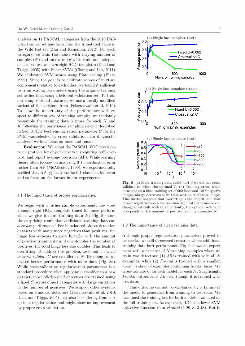
4.1 The importance of proper regularization

We begin with a rather simple experiment: how does

a single rigid HOG template tuned for faces perform

when we give it more training data N? Fig. 8 shows

the surprising result that additional training data can

decrease performance! For imbalanced object detection

datasets with many more negatives than positives, the

hinge loss appears to grow linearly with the amount

of positive training data; if one doubles the number of

positives, the total hinge loss also doubles. This leads to

overfitting. To address this problem, we found it crucial

to cross-validate C across different N . By doing so, we

do see better performance with more data (Fig. 8a).

While cross-validating regularization parameters is a

standard procedure when applying a classifier to a new

dataset, most off-the-shelf detectors are trained using

a fixed C across object categories with large variations

in the number of positives. We suspect other systems

based on standard detectors (Felzenszwalb et al, 2010;

Dalal and Triggs, 2005) may also be suffering from sub-

optimal regularization and might show an improvement

by proper cross-validation.

(a) Single face template (test)

(b) Single face template (train)

(c) Single face template (test)

Fig. 8 (a) More training data could hurt if we did not cross-validate to select the optimal C. (b) Training error, whenmeasured on a fixed training set of 900 faces and 1218 negativeimages, always decreases as we train with more of those images.This further suggests that overfitting is the culprit, and thatproper regularization is the solution. (c) Test performance canchange drastically with C. Importantly, the optimal setting ofC depends on the amount of positive training examples N .

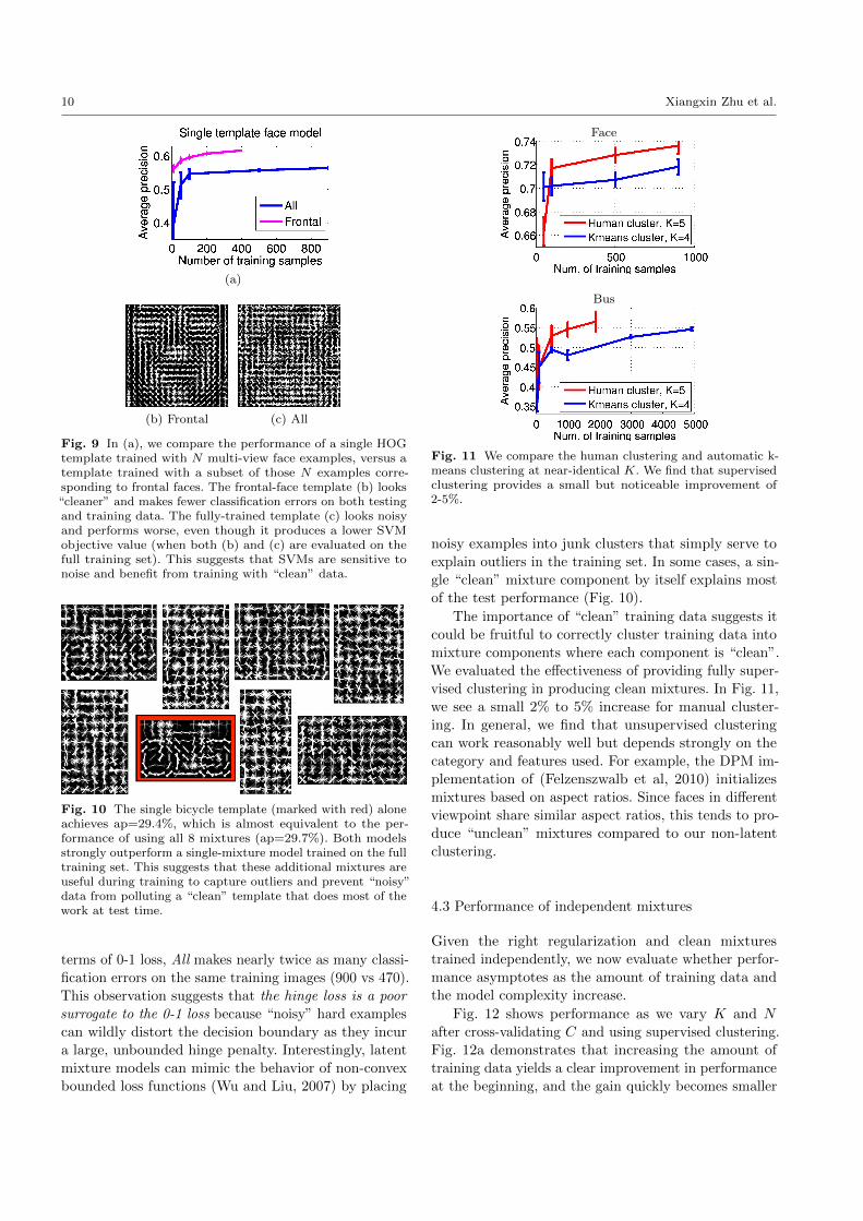
4.2 The importance of clean training data

Although proper regularization parameters proved to

be crucial, we still discovered scenarios where additional

training data hurt performance. Fig. 9 shows an experi-

ment with a fixed set of N training examples where we

train two detectors: (1) All is trained with with all N

examples, while (2) Frontal is trained with a smaller,“clean” subset of examples containing frontal faces. We

cross-validate C for each model for each N . Surprisingly,

Frontal outperforms All even though it is trained with

less data.

This outcome cannot be explained by a failure of

the model to generalize from training to test data. We

examined the training loss for both models, evaluated on

the full training set. As expected, All has a lower SVM

objective function than Frontal (1.29 vs 3.48). But in

10 Xiangxin Zhu et al.

(a)

(b) Frontal (c) All

Fig. 9 In (a), we compare the performance of a single HOGtemplate trained with N multi-view face examples, versus atemplate trained with a subset of those N examples corre-sponding to frontal faces. The frontal-face template (b) looks“cleaner” and makes fewer classification errors on both testingand training data. The fully-trained template (c) looks noisyand performs worse, even though it produces a lower SVMobjective value (when both (b) and (c) are evaluated on thefull training set). This suggests that SVMs are sensitive tonoise and benefit from training with “clean” data.

Fig. 10 The single bicycle template (marked with red) aloneachieves ap=29.4%, which is almost equivalent to the per-formance of using all 8 mixtures (ap=29.7%). Both modelsstrongly outperform a single-mixture model trained on the fulltraining set. This suggests that these additional mixtures areuseful during training to capture outliers and prevent “noisy”data from polluting a “clean” template that does most of thework at test time.

terms of 0-1 loss, All makes nearly twice as many classi-

fication errors on the same training images (900 vs 470).

This observation suggests that the hinge loss is a poor

surrogate to the 0-1 loss because “noisy” hard examples

can wildly distort the decision boundary as they incur

a large, unbounded hinge penalty. Interestingly, latent

mixture models can mimic the behavior of non-convex

bounded loss functions (Wu and Liu, 2007) by placing

Face

Bus

Fig. 11 We compare the human clustering and automatic k-means clustering at near-identical K. We find that supervisedclustering provides a small but noticeable improvement of2-5%.

noisy examples into junk clusters that simply serve to

explain outliers in the training set. In some cases, a sin-

gle “clean” mixture component by itself explains most

of the test performance (Fig. 10).

The importance of “clean” training data suggests it

could be fruitful to correctly cluster training data intomixture components where each component is “clean”.

We evaluated the effectiveness of providing fully super-

vised clustering in producing clean mixtures. In Fig. 11,

we see a small 2% to 5% increase for manual cluster-

ing. In general, we find that unsupervised clustering

can work reasonably well but depends strongly on the

category and features used. For example, the DPM im-

plementation of (Felzenszwalb et al, 2010) initializes

mixtures based on aspect ratios. Since faces in different

viewpoint share similar aspect ratios, this tends to pro-

duce “unclean” mixtures compared to our non-latent

clustering.

4.3 Performance of independent mixtures

Given the right regularization and clean mixtures

trained independently, we now evaluate whether perfor-mance asymptotes as the amount of training data and

the model complexity increase.

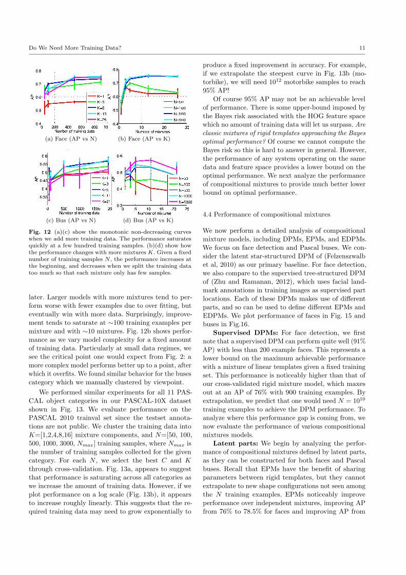
Fig. 12 shows performance as we vary K and N

after cross-validating C and using supervised clustering.

Fig. 12a demonstrates that increasing the amount of

training data yields a clear improvement in performance

at the beginning, and the gain quickly becomes smaller

Do We Need More Training Data? 11

(a) Face (AP vs N) (b) Face (AP vs K)

(c) Bus (AP vs N) (d) Bus (AP vs K)

Fig. 12 (a)(c) show the monotonic non-decreasing curveswhen we add more training data. The performance saturatesquickly at a few hundred training samples. (b)(d) show howthe performance changes with more mixtures K. Given a fixednumber of training samples N , the performance increases atthe beginning, and decreases when we split the training datatoo much so that each mixture only has few samples.

later. Larger models with more mixtures tend to per-

form worse with fewer examples due to over fitting, but

eventually win with more data. Surprisingly, improve-

ment tends to saturate at ∼100 training examples per

mixture and with ∼10 mixtures. Fig. 12b shows perfor-

mance as we vary model complexity for a fixed amount

of training data. Particularly at small data regimes, we

see the critical point one would expect from Fig. 2: a

more complex model performs better up to a point, after

which it overfits. We found similar behavior for the buses

category which we manually clustered by viewpoint.

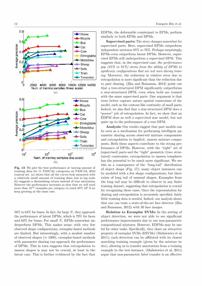
We performed similar experiments for all 11 PAS-

CAL object categories in our PASCAL-10X dataset

shown in Fig. 13. We evaluate performance on the

PASCAL 2010 trainval set since the testset annota-

tions are not public. We cluster the training data into

K=[1,2,4,8,16] mixture components, and N=[50, 100,

500, 1000, 3000, Nmax] training samples, where Nmax is

the number of training samples collected for the given

category. For each N , we select the best C and K

through cross-validation. Fig. 13a, appears to suggest

that performance is saturating across all categories as

we increase the amount of training data. However, if we

plot performance on a log scale (Fig. 13b), it appears

to increase roughly linearly. This suggests that the re-

quired training data may need to grow exponentially to

produce a fixed improvement in accuracy. For example,

if we extrapolate the steepest curve in Fig. 13b (mo-

torbike), we will need 1012 motorbike samples to reach

95% AP!

Of course 95% AP may not be an achievable level

of performance. There is some upper-bound imposed by

the Bayes risk associated with the HOG feature space

which no amount of training data will let us surpass. Are

classic mixtures of rigid templates approaching the Bayes

optimal performance? Of course we cannot compute the

Bayes risk so this is hard to answer in general. However,the performance of any system operating on the same

data and feature space provides a lower bound on the

optimal performance. We next analyze the performance

of compositional mixtures to provide much better lower

bound on optimal performance.

4.4 Performance of compositional mixtures

We now perform a detailed analysis of compositional

mixture models, including DPMs, EPMs, and EDPMs.

We focus on face detection and Pascal buses. We con-

sider the latent star-structured DPM of (Felzenszwalb

et al, 2010) as our primary baseline. For face detection,

we also compare to the supervised tree-structured DPM

of (Zhu and Ramanan, 2012), which uses facial land-

mark annotations in training images as supervised part

locations. Each of these DPMs makes use of different

parts, and so can be used to define different EPMs and

EDPMs. We plot performance of faces in Fig. 15 and

buses in Fig.16.

Supervised DPMs: For face detection, we first

note that a supervised DPM can perform quite well (91%

AP) with less than 200 example faces. This represents a

lower bound on the maximum achievable performance

with a mixture of linear templates given a fixed training

set. This performance is noticeably higher than that of

our cross-validated rigid mixture model, which maxes

out at an AP of 76% with 900 training examples. By

extrapolation, we predict that one would need N = 1010

training examples to achieve the DPM performance. To

analyze where this performance gap is coming from, we

now evaluate the performance of various compositional

mixtures models.

Latent parts: We begin by analyzing the perfor-

mance of compositional mixtures defined by latent parts,

as they can be constructed for both faces and Pascal

buses. Recall that EPMs have the benefit of sharing

parameters between rigid templates, but they cannot

extrapolate to new shape configurations not seen among

the N training examples. EPMs noticeably improve

performance over independent mixtures, improving AP

from 76% to 78.5% for faces and improving AP from

12 Xiangxin Zhu et al.

(a)

(b)

Fig. 13 We plot the best performance at varying amount oftraining data for 11 PASCAL categories on PASCAL 2010trainval set. (a) shows that all the curves look saturated witha relatively small amount of training data; but in log scale(b) suggests a diminishing return instead of true saturation.However the performance increases so slow that we will needmore than 1012 examples per category to reach 95% AP if wekeep growing at the same rate.

56% to 64% for buses. In fact, for large N , they approach

the performance of latent DPMs, which is 79% for faces

and 63% for buses. For small N , EPMs somewhat un-

derperform DPMs. This makes sense: with very few

observed shape configurations, exemplar-based methods

are limited. But interestingly, with a modest number

of observed shapes (≈ 1000), exemplar-based methods

with parameter sharing can approach the performance

of DPMs. This in turn suggests that extrapolation to

unseen shapes is may not be crucial, at least in the

latent case. This is further evidenced by the fact that

EDPMs, the deformable counterpart to EPMs, perform

similarly to both EPMs and DPMs.

Supervised parts: The story changes somewhat for

supervised parts. Here, supervised EPMs outperform

independent mixtures 85% to 76%. Perhaps surprisingly,

EPMs even outperform latent DPMs. However, super-

vised EPMs still underperform a supervised DPM. This

suggests that, in the supervised case, the performance

gap (85% vs 91%) stems from the ability of DPMs to

synthesize configurations that are not seen during train-

ing. Moreover, the reduction in relative error due to

extrapolation is more significant than the reduction due

to part sharing. (Zhu and Ramanan, 2012) point out

that a tree-structured DPM significantly outperforms

a star-structured DPM, even when both are trainedwith the same supervised parts. One argument is that

trees better capture nature spatial constraints of the

model, such as the contour-like continuity of small parts.

Indeed, we also find that a star-structured DPM does a

“poorer” job of extrapolation. In fact, we show that an

EDPM does as well a supervised star model, but not

quite up to the performance of a tree DPM.

Analysis: Our results suggest that part models can

be seen as a mechanism for performing intelligent pa-

rameter sharing across observed mixture components

and extrapolation to implicit, unseen mixture compo-

nents. Both these aspects contribute to the strong per-formance of DPMs. However, with the “right” set of

(supervised) parts and the “right” geometric (tree- struc-

tured) constraints, extrapolation to unseen templates

has the potential to be much more significant. We see

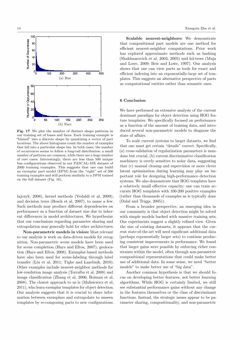
this as a consequence of the “long-tail” distribution

of object shape (Fig. 17); many object instances canbe modeled with a few shape configurations, but there

exists of long tail of unusual shapes. Examples from

the long tail may be difficult to observe in any finite

training dataset, suggesting that extrapolation is crucial

for recognizing these cases. Once the representation for

sharing and extrapolation is accurately specified, fairly

little training data is needed. Indeed, our analysis shows

that one can train a state-of-the-art face detector (Zhu

and Ramanan, 2012) with 50 face images.

Relation to Exemplar SVMs: In the setting of

object detection, we were not able to see significant

performance improvements due to our non-parametric

compositional mixtures. However, EDPMs may be use-

ful for other tasks. Specifically, they share an attractive

property of exemplar SVMs (ESVMs) (Malisiewicz et al,

2011): each detection can be affiliated with its closest

matching training example (given by the mixture in-

dex), allowing us to transfer annotations from a training

example to the test instance. (Malisiewicz et al, 2011)

argue that non-parametric label transfer is an effective

Do We Need More Training Data? 13

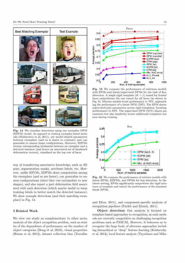
Fig. 14 We visualize detections using our exemplar DPM(EDPM) model. As opposed to existing exemplar-based meth-ods (Malisiewicz et al, 2011), our model shared parametersbetween exemplars (and so is faster to evaluate) and cangeneralize to unseen shape configurations. Moreover, EDPMsreturns corresponding landmarks between an exemplar and adetected instance (and hence an associated set of landmarkdeformation vectors), visualized on the top row of faces.

way of transferring associative knowledge, such as 3D

pose, segmentation masks, attribute labels, etc. How-

ever, unlike ESVMs, EDPMs share computation among

the exemplars (and so are faster), can generalize to un-

seen configurations (since they can extrapolate to new

shapes), and also report a part deformation field associ-

ated with each detection (which maybe useful to warp

training labels to better match the detected instance).

We show example detections (and their matching exem-

plars) in Fig. 14.

5 Related Work

We view our study as complementary to other meta-

analysis of the object recognition problem, such as stud-

ies of the dependence of performance on the number of

object categories (Deng et al, 2010), visual properties

(Hoiem et al, 2012), dataset collection bias (Torralba

Faces

Fig. 15 We compare the performance of mixtures modelswith EPMs and latent/supervised DPMs for the task of facedetection. A single rigid template (K = 1) tuned for frontalfaces outperforms the one tuned for all faces (as shown inFig. 9). Mixture models boost performance to 76%, approach-ing the performance of a latent DPM (79%). The EPM sharessupervised part parameters across rigid templates, boostingperformance to 85%. The supervised DPM (91%) shares pa-rameters but also implicitly scores additional templates notseen during training.

Bus

Fig. 16 We compare the performance of mixture models withlatent EPMs, EDPMs, and DPMs for bus detection. In thelatent setting, EPMs significantly outperform the rigid mix-tures of template and match the performance of the standardlatent DPMs.

and Efros, 2011), and component-specific analysis of

recognition pipelines (Parikh and Zitnick, 2011).

Object detection: Our analysis is focused on

template-based approaches to recognition, as such meth-

ods are currently competitive on challenging recognition

problems such as PASCAL. However, it behooves us to

recognize the large body of alternate approaches includ-

ing hierarchical or “deep” feature learning (Krizhevsky

et al, 2012), local feature analysis (Tuytelaars and Miko-

14 Xiangxin Zhu et al.

(a) Bus

(b) Face

Fig. 17 We plot the number of distinct shape patterns inour training set of buses and faces. Each training example is“binned” into a discrete shape by quantizing a vector of partlocations. The above histograms count the number of examplesthat fall into a particular shape bin. In both cases, the numberof occurrences seems to follow a long-tail distribution: a smallnumber of patterns are common, while there are a huge numberof rare cases. Interestingly, there are less than 500 uniquebus configurations observed in our PASCAL-10X dataset of2000 training examples. This suggests that one can buildan exemplar part model (EPM) from the “right” set of 500training examples and still perform similarly to a DPM trainedon the full dataset (Fig. 16).

lajczyk, 2008), kernel methods (Vedaldi et al, 2009),

and decision trees (Bosch et al, 2007), to name a few.

Such methods may produce different dependencies on

performance as a function of dataset size due to inher-

ent differences in model architectures. We hypothesize

that our conclusions regarding parameter sharing and

extrapolation may generally hold for other architectures.

Non-parametric models in vision: Most relevant

to our analysis is work on data-driven models for recog-

nition. Non-parametric scene models have been used

for scene completion (Hays and Efros, 2007), geoloca-

tion (Hays and Efros, 2008). Exemplar-based methods

have also been used for scene-labeling through label

transfer (Liu et al, 2011; Tighe and Lazebnik, 2010).

Other examples include nearest-neighbor methods for

low-resolution image analysis (Torralba et al, 2008) and

image classification (Zhang et al, 2006; Boiman et al,

2008). The closest approach to us is (Malisiewicz et al,

2011), who learn exemplar templates for object detection.

Our analysis suggests that it is crucial to share infor-

mation between exemplars and extrapolate to unseen

templates by re-composing parts to new configurations.

Scalable nearest-neighbors: We demonstrate

that compositional part models are one method for

efficient nearest-neighbor computations. Prior work

has explored approximate methods such as hashing

(Shakhnarovich et al, 2003, 2005) and kd-trees (Muja

and Lowe, 2009; Beis and Lowe, 1997). Our analysis

shows that one can view parts as tools for exact and

efficient indexing into an exponentially-large set of tem-

plates. This suggests an alternative perspective of parts

as computational entities rather than semantic ones.

6 Conclusion

We have performed an extensive analysis of the current

dominant paradigm for object detection using HOG fea-

ture templates. We specifically focused on performance

as a function of the amount of training data, and intro-

duced several non-parametric models to diagnose the

state of affairs.

To scale current systems to larger datasets, we find

that one must get certain “details” correct. Specifically,

(a) cross-validation of regularization parameters is mun-

dane but crucial, (b) current discriminative classificationmachinery is overly sensitive to noisy data, suggesting

that (c) manual cleanup and supervision or more clever

latent optimization during learning may play an im-

portant role for designing high-performance detection

systems. We also demonstrate that HOG templates have

a relatively small effective capacity; one can train ac-

curate HOG templates with 100-200 positive examples

(rather than thousands of examples as is typically done

(Dalal and Triggs, 2005)).

From a broader perspective, an emerging idea in

our community is that object detection might be solved

with simple models backed with massive training sets.

Our experiments suggest a slightly refined view. Given

the size of existing datasets, it appears that the cur-

rent state-of-the-art will need significant additional data

(perhaps exponentially larger sets) to continue produc-

ing consistent improvements in performance. We found

that larger gains were possible by enforcing richer con-

straints within the model, often through non-parametric

compositional representations that could make better

use of additional data. In some sense, we need “better

models” to make better use of “big data”.

Another common hypothesis is that we should fo-

cus on developing better features, not better learning

algorithms. While HOG is certainly limited, we still

see substantial performance gains without any change

in the features themselves or the class of discriminant

functions. Instead, the strategic issues appear to be pa-

rameter sharing, compositionality, and non-parametric

Do We Need More Training Data? 15

encodings. Establishing and using accurate, clean corre-

spondence among training examples (e.g., that specify

that certain examples belong to the same sub-category,

or that certain spatial regions correspond to the same

part) and developing non-parametric compositional ap-

proaches that implicitly make use of augmented training

sets appear the most promising directions.

References

Beis JS, Lowe DG (1997) Shape indexing using approx-

imate nearest-neighbour search in high-dimensional

spaces. In: Computer Vision and Pattern Recognition,1997. Proceedings., 1997 IEEE Computer Society Con-

ference on, IEEE, pp 1000–1006

Boiman O, Shechtman E, Irani M (2008) In defense of

nearest-neighbor based image classification. In: Com-puter Vision and Pattern Recognition, 2008. CVPR

2008. IEEE Conference on, IEEE, pp 1–8

Bosch A, Zisserman A, Muoz X (2007) Image classifi-

cation using random forests and ferns. In: Computer

Vision, 2007. ICCV 2007. IEEE 11th International

Conference on, IEEE, pp 1–8

Bourdev L, Malik J (2009) Poselets: Body part detec-

tors trained using 3d human pose annotations. In:

International Conference on Computer Vision

Chang C, Lin C (2011) LIBSVM: A library for support

vector machines. ACM Transactions on Intelligent Sys-

tems and Technology 2:27:1–27:27, software available

at http://www.csie.ntu.edu.tw/~cjlin/libsvm

Dalal N, Triggs B (2005) Histograms of oriented gradi-

ents for human detection. In: CVPR 2005.

Deng J, Berg A, Li K, Fei-Fei L (2010) What Does

Classifying More Than 10,000 Image Categories Tell

Us? In: International Conference on Computer Vision

Divvala SK, Efros AA, Hebert M (2012) How impor-

tant are deformable parts in the deformable parts

model? In: European Conference on Computer Vision

(ECCV), Parts and Attributes Workshop

Everingham M, Van Gool L, Williams C, Winn J, Zis-

serman A (2010) The PASCAL visual object classes

(VOC) challenge. International Journal of Computer

Vision 88(2):303–338

Felzenszwalb P, Huttenlocher D (2012) Distance trans-

forms of sampled functions. Theory of Computing

8(19)

Felzenszwalb P, Girshick R, McAllester D, Ramanan D

(2010) Object detection with discriminatively trained

part-based models. IEEE TPAMI

Gross R, Matthews I, Cohn J, Kanade T, Baker S (2010)

Multi-pie. Image and Vision Computing

Halevy A, Norvig P, Pereira F (2009) The unreason-

able effectiveness of data. Intelligent Systems, IEEE

24(2):8–12

Hays J, Efros A (2007) Scene completion using millions

of photographs. In: ACM Transactions on Graphics

(TOG), ACM, vol 26, p 4

Hays J, Efros AA (2008) Im2gps: estimating geographic

information from a single image. In: Computer Vision

and Pattern Recognition, 2008. CVPR 2008. IEEE

Conference on, IEEE, pp 1–8

Hoiem D, Chodpathumwan Y, Dai Q (2012) Diagnosingerror in object detectors. In: Computer Vision ECCV

2012, Springer Berlin Heidelberg, vol 7574, pp 340–353

Krizhevsky A, Sutskever I, Hinton G (2012) Imagenet

classification with deep convolutional neural networks.

In: Advances in Neural Information Processing Sys-

tems 25, pp 1106–1114

Liu C, Yuen J, Torralba A (2011) Nonparametric scene

parsing via label transfer. Pattern Analysis and Ma-

chine Intelligence, IEEE Transactions on 33(12):2368–

2382

Malisiewicz T, Gupta A, Efros A (2011) Ensemble of

exemplar-svms for object detection and beyond. In:

International Conference on Computer Vision, IEEE,

pp 89–96

McAllester DA (1999) Some pac-bayesian theorems. Ma-

chine Learning 37(3):355–363

Muja M, Lowe DG (2009) Fast approximate nearest

neighbors with automatic algorithm configuration. In:

International Conference on Computer Vision Theory

and Applications (VISSAPP09), pp 331–340

Parikh D, Zitnick C (2011) Finding the weakest link in

person detectors. In: Computer Vision and PatternRecognition, IEEE, pp 1425–1432

Platt J (1999) Probabilistic outputs for support vec-

tor machines and comparisons to regularized likeli-

hood methods. In: ADVANCES IN LARGE MARGIN

CLASSIFIERS, MIT Press, pp 61–74Shakhnarovich G, Viola P, Darrell T (2003) Fast pose

estimation with parameter-sensitive hashing. In: Com-

puter Vision, 2003. Proceedings. Ninth IEEE Interna-

tional Conference on, IEEE, pp 750–757

Shakhnarovich G, Darrell T, Indyk P (2005) Nearest-

neighbor methods in learning and vision: theory and

practice, vol 3. MIT press Cambridge

Tighe J, Lazebnik S (2010) Superparsing: scalable non-

parametric image parsing with superpixels. In: Com-

puter Vision–ECCV 2010, Springer, pp 352–365

Torralba A, Efros A (2011) Unbiased look at dataset

bias. In: Computer Vision and Pattern Recognition,

IEEE, pp 1521–1528

Torralba A, Fergus R, Freeman WT (2008) 80 million

tiny images: A large data set for nonparametric object

16 Xiangxin Zhu et al.

and scene recognition. Pattern Analysis and Machine

Intelligence, IEEE Transactions on 30(11):1958–1970

Tuytelaars T, Mikolajczyk K (2008) Local invariant

feature detectors: a survey. Foundations and Trends R©in Computer Graphics and Vision 3(3):177–280

Vedaldi A, Gulshan V, Varma M, Zisserman A (2009)

Multiple kernels for object detection. In: Computer

Vision, 2009 IEEE 12th International Conference on,

IEEE, pp 606–613

Wu Y, Liu Y (2007) Robust truncated hinge loss support

vector machines. Journal of the American StatisticalAssociation 102(479):974–983

Zhang H, Berg AC, Maire M, Malik J (2006) Svm-

knn: Discriminative nearest neighbor classification for

visual category recognition. In: Computer Vision and

Pattern Recognition, 2006 IEEE Computer Society

Conference on, IEEE, vol 2, pp 2126–2136

Zhu X, Ramanan D (2012) Face detection, pose esti-

mation, and landmark localization in the wild. In:

Computer Vision and Pattern Recognition