Do Stock Market Investors Understand the Risk

Sentiment of Corporate Annual Reports? ∗

Feng Li

Stephen M. Ross School of Business, University of Michigan

701 Tappan St., Ann Arbor, MI 48109

Phone: (734)936-2771

Email: Feng@umich.edu

First Draft: August 2005

This Draft: April 21, 2006

∗This paper was previously titled “The implications of annual report’s risk sentiment for future earnings

and stock returns”. I acknowledge the financial support of the Harry Jones Endowment for Research on

Earnings Quality at the Ross School of Business, University of Michigan. I thank Jason Chen, Shijun Cheng,

Patty Dechow, Ilia Dichev, Michelle Hanlon, Yu Huang, Gene Imhoff, Roby Lehavy, Michal Matejka, Venky

Nagar, Richard Sloan, Suraj Srinivasan, and the workshop participants at the University of Michigan for

their comments. All errors remain mine.

Abstract

I test the stock market efficiency with respect to the information in the texts of an-

nual reports. More specifically, I examine the implications of corporate annual reports’

risk sentiment for future earnings and stock returns. I measure the risk sentiment of

annual reports by counting the frequency of words related to risk or uncertainty in the

10-K filings. I find that an increase in risk sentiment is associated with lower future

earnings: Firms with a larger increase in risk sentiment have more negative earnings

changes in the next year. Risk sentiment of annual reports can predict future returns

in a cross-sectional setting: Firms with a large increase in risk sentiment experience

significantly negative returns relative to those firms with little increase in risk senti-

ment in the twelve months after the annual report filing date. A hedge portfolio based

on buying firms with a minor increase in risk sentiment of annual reports and shorting

firms with a large increase in risk sentiment generates an annual Alpha of more than

10% measured using the four-factor model including the Fama-French three factors

and the momentum factor.

1

1 Introduction

This paper tests the efficiency of stock market with respect to the information contained in

the texts of publicly available documents. In particular, I study the implications of corporate

annual report’s risk sentiment (i.e., its emphasis on risk and uncertainty) for future earnings

and stock returns.

There are a large number of studies in finance and accounting that document empirical

regularities on the association between public information and future stock returns. The

information set examined includes financial or market variables such as size, book-to-market

ratio, accruals, corporate investment, past stock returns, and analyst forecast, among others.

Other studies explore future returns following firm events, such as earnings announcement,

IPO, SEO, and merger and acquisitions.

However, very few studies examine the relation between information extracted from the

texts of publicly available documents and stock returns.1 In today’s world, a huge amount

of information is stored as text instead of numeric data (Nasukawa and Nagano (2001)).

Information retrieval and knowledge discovery from textual data thus provide an alternative

methodology for research. Indeed, text-based analysis, as opposed to pure data analysis, has

been gaining popularity in various research fields, including biology (e.g., protein interac-

tion generation by Rindflesch, Hunter, and Aronson (1999)), medical science (e.g., forming

hypotheses about disease by Swanson (1987)), and sociology (e.g., uncovering social impact

by Narin, Hamilton, and Olivastro (1997)).

Text-based information is likely to contain factors relevant to equity prices. For instance,

a typical corporate annual report includes many pages of management discussion and foot-

notes to the financial statements. While almost all the numbers in the financial statements

are historical and backward-looking, texts in corporate annual reports can contain forward-

looking information. For example, in the MD&A (Management Discussion & Analysis)

1One exception is the literature on Internet stock message boards (e.g., Antweiler and Frank (2004)),

which examines the relation between information from Internet discussion board and stock returns and

volatility.

2

section of annual reports, managers may discuss factors related to consumer demand and

competition. Therefore, information extracted from the text portion of corporate annual

reports can potentially contain incremental information about firms’ future performance.

Examining whether stock prices reflect the information contained in the texts of publicly

available documents offers several advantages to test market efficiency theory compared with

the traditional tests based on numeric data. First, public text information provides a setting

more consistent with the argument of limited investor rationality and investor attention

developed in the recent literature (Shleifer (2000) and Hirshleifer and Teoh (2003)). A

puzzling observation for the behavioral explanations for the stock return anomalies is that

many empirical regularities on stock returns still exist without being arbitraged away after

being documented for a long time. This point is especially salient for anomalies based on very

simple financial data, such as book-to-market and accruals. After they are published and

widely studied by academic researchers, the information processing cost should be relatively

low for these factors. Hence, numeric data extracted from financial statements or stock

market seem unlikely to be subject to simple stories of limited investor attention.

Compared with simple numeric data, textual information is presumably more costly

to process. For instance, on average, the annual reports filed by U.S. public companies

analyzed in this paper contain 70,279 words and the median length is 41,973 words. To ex-

tract information from these documents systematically involves non-trivial amount of effort.

Therefore, public text information provides a setting more consistent with the argument of

limited investors rationality and investor attention assumptions developed in the recent lit-

erature. Linking text-based information with stock returns thus provides another interesting

perspective to test market efficiency theory.

Second, many of the existing number-based anomalies are highly correlated. As a result,

some authors have suggested that the same empirical regularity is discovered many times in

different settings and interpreted as different anomalies. This is evidenced by the collinearity

of the return-related factors in Fama and French (2005). The collinearity of the number-based

variables casts doubt on the independence of the large number of studies in the literature.

3

Variables based on the texts in financial statements can potentially offer more orthogonal

factors and provide a more independent test of market efficiency.

Finally, text-based data may provide additional richness for researchers to test market

efficiency. For instance, as part of management disclosure, the texts in financial statements

can be strategic and reflect managers’ opportunistic behavior. Managers are likely to have

more degrees of freedom in writing the texts of the annual report than the numbers, since the

latter are subject to Generally Accepted Accounting Principles. Therefore, investors need

to understand managerial behavior and strategic intent to fully understand the implications

of published disclosure. The power of the market efficiency tests can be improved if the

strategic nature of the published disclosure can be exploited (e.g., Sloan (1996)).

This paper examines whether the stock market is efficient with respect to an important

source of public information – text in the financial statements. I focus on the annual reports’

emphasis on risk. I measure the emphasis on risk in annual reports by counting the frequency

of words related to risk or uncertainty (“risk sentiment”) in the whole 10-K document. In

the MD&A (Management Discussion & Analysis) section of the annual reports, managers

are required to discuss the risks associated with operations. Typical risks discussed include

operating risk, credit risk, interest rate risk, and currency risk. But the discussion is not

limited to the MD&A section. In other parts of the annual report (e.g., notes to the financial

statements), managers may voluntarily discuss more risk-related issues such as contingent

litigation.

There are several reasons why an emphasis on risk by managers may signal poor per-

formance in the future. When discussing the future outlook of firms, managers tend to use

more vague language for bad news. For instance, Skinner (1994) finds that good news dis-

closures by managers tend to be point or range estimates of future EPS, while bad news

disclosures tend to be qualitative statements. Consistent with this, managers rarely discuss

future performance in an absolutely pessimistic tone in the annual reports. Many forward-

looking statements in the annual reports are written with words such as “may”, “might”, or

“could”. They are also likely to use soft words such as “risk” or “uncertain” to describe ad-

4

verse information about future performance. The emphasis on firm operating or other risks

is an alternative approach for managers to present their pessimistic views about future. All

else equal, more emphasis on risk factors may therefore signal lower managerial confidence

about the future.2

More importantly, managers have incentives to disclose their pessimistic views about

the future of the firm in annual reports. Skinner (1994) and Skinner (1997) show that

managers use voluntary disclosures to preempt large, negative earnings surprises more often

than other types of earnings news. To avoid ex post shareholder litigation related to poor

earnings, managers are likely to emphasize the future risks in the annual reports if they

anticipate bad earnings news in the future.

Consistent with the argument that the emphasis on risk signals poor future performance,

I find that an increase in the risk sentiment of annual report is associated with significantly

lower future earnings. Firms in the quintile with the largest increase in annual report risk

sentiment this year experience a change in earnings (scaled by book value of assets) of more

than 0.02 lower than those in the quintile of the lowest risk sentiment increase.

The change of the risk sentiment is also negatively related to future returns in a cross-

section. The effect holds after controlling for market, size, book-to-market, and momentum.

More importantly, this effect remains significant even after controlling for other variables

that are commonly used to predict future earnings. I include all the variables in Fama and

French (2005) in the cross-sectional regression of future returns on risk sentiment increase

and the negative association still remains.

The time-series evidence confirms this finding. A hedge portfolio based on buying firms

with a minor increase in risk sentiment and shorting those with a significant increase gen-

erates an annual Alpha of more than 10% based on the four-factor model including Fama-

French three factors and the momentum factor. The relation between risk sentiment and

2The “risk” as typically used by managers is not the same as the covariance concept in asset pricing

models. Rather, it mostly refers to the cash flow volatility. For instance, the “credit risks” discussed in

annual reports typically are related to future uncollectible receivables.

5

future returns is also robust to arrays of robustness checks.

The evidence in this paper suggests that the stock market does not fully reflect the in-

formation contained in the texts of annual reports about future profitability. This finding

adds another piece of evidence of possible market inefficiency to the literature. However,

a caveat is in order. Using a tautological valuation framework, Fama and French (2005)

argue that three variables are related to expected returns: the book-to-market equity ratio,

expected profitability, and expected investment. Hence, according to them, any variable(s)

that can predict future earnings may predict future stock returns simply because they are

correlated with the (unobserved) expected returns. Their argument provides an alternative

but rational explanation for all investment strategies based on fundamental analysis. Em-

pirically, however, absent a widely accepted asset pricing model, it is difficult to directly test

the rational versus the irrational explanation. This caveat certainly applies to this study.

The remainder of the paper proceeds as follows. Section 2 discusses empirical measures

of annual report risk sentiment and summary statistics. In Section 3, I present the basic

empirical findings on the association of risk sentiment and future earnings and stock returns.

Section 4 discusses the findings and does some additional tests. Section 5 concludes.

2 Data and Empirical Measure of the Risk Sentiment

2.1 Data

Following Li (2006), I collect my sample as follows: (1) I start with the intersection of CRSP-

COMPUSTAT non-financial firm-years. Financial firms (industry code between 6000 and

6999) are dropped because risk-related words have different implications for these firms. (2)

I then manually match GVKEY (from COMPUSTAT) with the Central Index Key (CIK)

used by the SEC online Edgar system using firm name and other firm characteristics. Firms

without matching CIK are dropped. To get stock returns that are based on PERMNO, I

rely on the GVKEY-PERMNO link file in the CRSP-COMPUSTAT merged database. (3) I

download from Edgar the 10-K filing for every remaining firm-year. Those firm-years that do

6

not have electronic 10-K filings on Edgar are then excluded.3 (4) For each 10-K file, all the

heading items, paragraphs that have fewer than one line, and tables are deleted. (5) Firms

with no risk-related words in this or last fiscal year are dropped. The SEC requires firms

to include an MD&A section in their 10-K filing with a discussion of business and financial

risks. Therefore, the documents without a single occurrence of risk-related words are likely

to be unusual documents such as Amendment to the 10-K filings.

My final sample consists of 34,180 firm-years with annual reports filing dates between

calendar years 1994 and 2005. Since December fiscal-year end firms typically file their annual

reports in the next calendar year, my sample mostly covers fiscal year 1993 to 2004. Sample

size varies in the empirical tests depending on the data requirement. For instance, in the tests

linking risk sentiment with future earnings, most of the fiscal year 2004 data are dropped

because the financial numbers for fiscal 2005 are not available yet.

2.2 Measure of Risk Sentiment

To measure the emphasis on risk and uncertainty of the annual reports, I simply count

the number of occurences of the risk-related words. In particular, I count the frequencies

of “risk” (including “risk”, “risks”, and “risky”) and “uncertainty” (including “uncertain”,

“uncertainty”, and “uncertainties”). Since many firms have disclosure about risk-free interest

rate (e.g., in their stock option compensation note), any words in the format of “risk-” are

excluded in the count. Confounding strings such as “asterisk” are also excluded.

My approach is simple but effective. To better capture the risk sentiment of a document

in a more precise way would require much more detailed assumptions about the context and

the linguistic structure. There are some rough methods in computational linguistics to do

this, but the cost seems to outweigh the benefit. For instance, Turney (2002) uses a simple

unsupervised learning algorithm to classify customer reviews of products on epinions.com

into positive and negative. Even though the reviews are much shorter than annual reports,

the classification algorithm does a very poor job for some categories (e.g., the accuracy rate

3SEC has electronic Edgar filing available online from 1994.

7

for movie reviews is only 66%, not much higher than a 50-50 random classification). In a

general setting such as annual reports, which cover perhaps all industries in the economy, a

context-specific measure of risks seems to be difficult to establish at this stage.

I define risk sentiment as

RSt = ln(1 + NRt), (1)

and change of risk sentiment as

∆RSt = ln(1 + NRt) − ln(1 + NRt−1), (2)

where NRt and NRt−1 are the numbers of occurences of risk-related words in year t and

year t− 1 respectively.

2.3 An Example: Ford Motor Co.

To gain some intuition on the risk sentiment measure, the Appendix provides an example

using the disclosures of Ford Motor Co. Table A1 in the Appendix shows the risk sentiment

measures, earnings, and the twelve-month stock returns following the annual report filing

date of Ford for each fiscal year from 1993 to 2003. The focus here is on fiscal 2000, in which

there is a dramatic change in risk sentiment in the annual report.

The earnings of fiscal 2000 is not unusual. The return on assets (ROA) of fiscal year 2000

is 0.023, not quite different from that of 1999 (0.026). The stock returns in 2000, computed

as the twelve-month returns starting from the month after fiscal 1999 annual report filing

date, is 54% after adjusting for the market and is actually much better than the previous

year (a market-adjusted return of -42%). Judged from the earnings and stock performance

in 1999 and 2000, it seems that fiscal 2001 should not be a bad year for Ford.

The risk sentiment change in the 2000 annual report, however, may tell a different story.

From 1993 to 1999, the number of risk-related words in Ford’s annual reports remains rel-

atively stable, ranging from 11 to 30. In the fiscal 2000 annual report, however, there are

99 occurences of risk-related words, an increase of more than 200% from the previous year.

8

A closer look at the annual reports confirms the calculation. For instance, one of the fac-

tors for the increase in risk sentiment is related to credit risks. As can be seen from the

Appendix, Item 7A (“Quantitative and Qualitative Disclosures About Market Risk”) takes

slightly more than one page in the 1999 annual report of Ford. In 2000, there are more than

five pages devoted to the same section. In 1999, only three categories of risks are discussed:

interest rate, foreign currency, and commodity price risks. In fiscal 2000, more than four

pages of discussions on credit risks are added in addition to the three types of risks disclosed

in the previous year. This suggests that Ford was much more worried about its future credit

losses at the end of fiscal 2000 than 1999. Another reason for the sharp increase in risk

sentiment is the litigation risk disclosure related to Firestone tires used on Ford Explorer.

Consistent with the hypothesis that a sharp increase in risk sentiment signals poor per-

formance in the future, the ROA of Ford in 2001 experiences a significant drop and becomes

negative (-0.02). The dramatic increase in the amount of discussion on credit risks in Ford’s

2000 annual report is followed by a significant increase in bad debt in 2001. A careful read

of 2001 annual reports reveals that the provision for credit losses increases by $1.7 billion

(increase from $1.7 billion in 2000 to $3.4 billion in 2001) during this year.

The stock price of Ford in 2001 is consistent with its performance. As the plot in Figure

A1 shows, on May 16, 2001, Ford announced that its European market would not break

even and its price tanked by more than 10% in a week. In August, Ford revealed that its

July sales dropped by 13% and the trial over Firestone tires on Ford SUVs also started on

August 14, 2001. These events triggered another drop of more than 10% in Ford’s stock

price. Overall, the market-adjusted stock return of Ford in the twelve-month period after

the 2000 annual report filing date is -41%.

Thus, the example of Ford confirms the intuition of my risk sentiment measure and the

hypothesis that the change in risk sentiment contains information about future performance.

Of course, the example is just a piece of anecdotal evidence. Formal evidence based on

statistical tests will be shown in Section 3.

9

2.4 Summary Statistics

Table 1 presents the summary statistics of the risk sentiment and some firm characteristics of

my sample. Since my sample covers almost the entire intersection of CRSP-COMPUSTAT,

there is a large variation in the size of the firms. The mean (median) market value of equity

at the end of the fiscal year is $1.42 billion ($175 million), with a standard deviation of $3.78

billion and an interquartile range of $757 million. Book-to-market ratio also has a large

dispersion across firms with a 25th percentile of 0.28 and a 75th percentile of 0.89.

Untabulated results show that 59.3% of my sample firms have a December fiscal year

end. On average, firms file their annual reports 88.5 days or 2.95 months after their fiscal

year end date. The mean number of words in the annual reports (after deleting headings and

financial statements etc. as described in the previous subsection) is 70,279 with a median of

41,973.

From Table 1, on average, there are 28 occurences of risk-related words (NR) in annual

reports. The change of the occurences (∆NRt = NRt − NRt−1) seems substantial, with

a mean of 3.30 (about 10% of the mean of NR level). The mean (median) change of risk

sentiment ∆RS is 0.15 (0.10). The standard deviation of ∆RS is 0.46 and the inter-quartile

range is 0.40, suggesting a substantial variation.

Table 2 shows the correlation of ∆RS with common firm characteristics using a regression

approach. The dependent variable is ∆RSt and the independent variables include ∆Et

(change in earnings, ∆Et = Et −Et−1, where E is earnings, #18 from Compustat, scaled by

beginning book value of assets, #6), lnMV Et (MV E is the market value of equity at the end

of fiscal year t, calculated as #25 times #199), and lnBTM (defined as natural logarithm of

book value of equity, #6 minus #181, divided by MV E). Year (the calendar year in which

an annual report is filed to the SEC) and two-digit SIC industry fixed effects are included

in the regression, but the coefficients on the industry fixed effects are not presented. All

the t-statistics are based on standard errors clustered by year to control for cross-sectional

correlation.

There is a negative correlation between the change of risk sentiment (∆RS) and this

10

year’s earnings, as evidenced by the coefficient of -0.033 on ∆E (t-statistic -5.32). Bigger

firms and growth firms tend to have more increase in risk sentiment: Coefficient on lnMV E

is 0.006 and that on lnBTM is -0.006. However, both coefficients are not statistically

significant. Most of the explanatory power comes from the year fixed effects. The combined

incremental R-squared of ∆E, lnMV E, lnBTM , and the industry fixed effects is only

0.3%. The incremental R-squared of the year fixed effects is about 6%. This suggests that

economy-level factors influence the change in the risk sentiment of firms’ annual reports.

The coefficients on the year fixed effects indicate that, for the sample as a whole, annual

reports filed in year 2000 and year 2001 (i.e., fiscal years 1999 and 2000 for December fiscal

year end firms) have the most negative change in risk sentiment. These happen to be the

years in which the stock market experienced a downward trend. It will be interesting to get

a longer time series to examine the relation between stock market performance and ∆RS.

Fama and French (2005) study a comprehensive set of variables documented in the lit-

erature that are shown to have power to predict future earnings and assets growth. These

variables are also included in the regression to examine their correlations with the change

in annual report risk sentiment. The variables include NegE (negative earnings dummy),

ROE, accruals (positive and negative accruals), assets growth, no-dividend dummy, dividend

to book equity ratio, OH (the bankruptcy score calculated from the Ohlson (1980)), and

PT (the fundamental strength variable calculated following Piotroski (2000)). The results in

column (2) indicate that ∆RS is correlated with many of the earnings-predicting variables

from the prior literature. Four of the nine variables are significantly correlated with ∆RS.

The rest show up insignificantly perhaps because of the potential multicollinearity between

the variables.

However, only two (AssG and PT ) of the four significant coefficients have signs consistent

with the possible argument that ∆RS may predict future earnings because of its correlations

with other earnings-predicting variables. AssG, the growth rate of total book assets, is

negatively related to future earnings (Fama and French (2005)). The positive correlation

between AssG and ∆RS (coefficient 0.020 with a t-value of 4.28) suggests that ∆RS may

11

also predict lower future earnings. PT is related to higher future earnings (Piotroski (2000)

and Fama and French (2005)) and ∆RS is negatively correlated with PT , suggesting that

they may capture similar underlying economic conditions of the firm.

The other two significant variables have the opposite signs. Prior studies find a negative

correlation between NegE, the loss dummy for year t, and future profitability. However,

NegE is negatively associated with ∆RS (coefficient on NegE of -0.030 with a t of -2.78),

suggesting that any possible negative correlation between ∆RS and future earnings is not

because of its correlation with NegE. Similarly, NoD, the no-dividend dummy, is shown to

be negatively related to future earnings but it has a negative correlation with ∆RS.

Overall, there is some correlation between ∆RS and the set of variables constructed

in previous studies. I will control for these variables when using ∆RS to predict future

profitability in later analysis.

3 Empirical Results

3.1 Future Earnings

This section examines the relation between changes in risk sentiment and future earnings.

Table 3 shows the regression results of next year’s earnings change ∆Et+1 on ∆RSt and

other control variables. In all the regressions, year and industry fixed effects are included. I

also include almost all the variables examined in Fama and French (2005) except the analyst

following variable, which will shrink the sample size a lot.4

In the univariate regression, ∆RSt is negatively and significantly related to ∆Et+1 with

a coefficient of -0.014 and a t-statistics of -5.61 with standard errors clustered at year level.

Adding all the controls to the regression dampens the coefficients a little, but the coefficient

on ∆RS is still negative and significant (-0.010 with a t of -3.91). The signs on most control

variables are consistent with previous literature and Fama and French (2005). For instance,

4Financial analysts’ forecast of earnings is included in Fama and French (2005) as a determinant of future

earnings and stock returns. I examine this in Section 4.7.

12

size (lnMV E), dividend (DTB), and PT are positively related to future earnings. Loss

dummy (NegE), +ACC (accruals for firms with positive accruals and 0 otherwise) , −ACC

(accruals for negative accruals and 0 otherwise), and growth (AssG) are related to lower

future earnings. Book-to-market ratio (lnBTM) and OH have the opposite signs with

Fama and French (2005), possibly because the dependent variable in my regressions is the

change, rather than the level, of next year’s earnings.

To see the effect more intuitively and take into consideration possible non-linearity effect,

I replace ∆RS with quintile dummies based on it. Every year, I sort firms into quintiles

based on the change in their annual report risk sentiment (∆RS). Four dummies (Q2 to Q5)

are created and included in the regression. Qi is defined as 1 if RS is in quintile i that year

and 0 otherwise. The results based on quintile dummies confirm the previous results based

on raw ∆RS. From table 3 panel A, it can be seen that the coefficients on Q2, Q3, Q4, and

Q5 are all negative, suggesting that relative to firms with the lowest ∆RS (i.e., Q1 firms),

firms in quintile 2 to 5 all have lower next year earnings changes. Moreover, as the quintile

number goes up, the coefficient becomes more negative, as evidenced by the monotonically

decreasing coefficients on Q2 to Q5. Adding the control variables makes the coefficient on

Q2 and Q3 positive and insignificantly different from zero. But Q4 and Q5 are still negative

and significant.

The negative correlation between ∆RS and future earnings solely comes from firms that

experience an increase in risk sentiment. Table 3 panel B shows the results of the regressions

by dividing firms into positive ∆RS and negative ∆RS. For positive ∆RS sample firms,

change of risk sentiment can predict lower future earnings (coefficient on ∆RS of -0.016 with

a t-value of -3.39) even after controlling for the variables in Fama and French (2005). Using

the quintile approach, the coefficients on Q2 to Q5 are -0.008 (t of -1.24), -0.018 (t of -2.96),

-0.012 (t of -2.56), and -0.023 (t of -3.66), almost monotonically decreasing.

From table 3 panel B, it is clear that there is no association between ∆RSt and ∆Et+1

for negative ∆RS firms. For negative ∆RS sample, ∆RS has a coefficient of 0.013 (t-value

0.86) when the controls are added. Results based on quintiles are similar: All the coefficients

13

on Q2 to Q5 are positive but insignificantly different from zero.

Overall, the finding in this section is that a larger increase in RS is associated with lower

future earnings, but a decrease in RS does not seem to have significant impact on future

earnings. A possible explanation for this is that the risk sentiment of annual report is more

likely to capture downside risk: Managers tend to discuss more about risks if they have

adverse information about future performance, but they do not deemphasize risk factors

even if they are optimistic about future profitability. This could be due to the asymmetric

incentives managers have to avoid ex post litigation. To mitigate litigation risks, managers

tend to be conservative and emphasize risks even when they are optimistic about future

performance.

3.2 Future returns

3.2.1 Cross-sectional evidence

I test for the relation between the change in annual report risk sentiment and future returns

in two steps, using both the cross-sectional regressions in this sub-section and the time-series

portfolio approach in the next sub-section. I first present cross-sectional regressions that link

future returns to ∆RS. I trace a firm’s stock returns in the twelve months after its annual

report filing date. For instance, if a firm files its fiscal 1999 annual report in March 2000,

I examine the relation between its ∆RS in fiscal 1999 and monthly stock returns between

April 2000 and March 2001. Essentially, every month I regress the monthly stock returns of

firm i (RETi) on its most recent ∆RS and control variables. The average of the coefficients

are then reported.

Because I do not find much evidence on the earnings predictive power of negative ∆RS,

I only focus on firm-years with positive ∆RS. I create a variable +∆RS, which equals ∆RS

if ∆RS is positive and 0 if a firm-year has a negative ∆RS. Table 4 presents the Fama-

MacBeth regression results. When +∆RS is used alone to explain returns, there is a strong

negative relation between average return and +∆RS. The average slope on +∆RS is -0.64

with a t-statistics of -4.04.

14

Although the coefficient on +∆RS is very significant, the average R-squared from the

Fama-MacBeth procedure is pretty low (0.001). Untabulated results show that if size (book-

to-market) is used alone to explain returns, the t-statistic is -2.56 (2.68) with an R-squared

of 0.010 (0.008). This suggests that, counter-intuitively, +∆RS is more significantly related

to returns than size or book-to-market, but it explains a smaller amount of variation in

returns. This is a consequence of the Fama-MacBeth procedure. In a univariate regression,

there is a monotonic relation between the regression R-squared and the t-statistic of the

slope: A higher t-statistic for the slope means that the independent variable explains more

variation in the dependent variable. In a Fama-MacBeth setting, however, this relation may

not hold. In our case, untabulated results show that size/book-to-market is significantly

related to returns in most months, but the sign of the coefficient flips. In other words, size

is negatively associated with future returns on average, but it is also often positively and

significantly related to returns. This leads to a high Fama-MacBeth R-squared, but a less

significant coefficient. On the other hand, +∆RS is either negatively or insignificantly related

to future returns and this results in a lower R-squared but a more significant coefficient.

Columns (2) and (3)show the relation between the variables used in prior studies and

future returns. When only size, book-to-market, and accruals are used to predict returns,

there is a negative relation between average returns and accruals (t=-1.32) and size (t=-1.48).

Book-to-market is positively related to future returns but the relation is not statistically

significant (t=1.00). Adding the variables from Fama and French (2005) to the regression

seems to make the coefficients become less significant. Of all the variables examined in Fama

and French (2005), only size (coefficient -0.18 with a t of -1.67), growth (AssG, coefficient of

-0.65 with a t of -4.35), and PT (coefficient of 0.10 with a t of 2.01) are significantly related

to future returns. Accruals is still negatively related to future returns, but it is statistically

insignificant (t=-0.49). This is likely due to the multicollinearity among the variables.

With all the control variables in the regression, +∆RS still predicts future returns neg-

atively (coefficient -0.45 with a t of -3.50 in column (4)). This is consistent with that ∆RS

captures information about future earnings that is more orthogonal to the information con-

15

tained in the variables based on financial or market numbers.

Table 4 panel B shows the results of regressing future returns on ∆RS using positive

∆RS sample firms only. The magnitude of the coefficient on ∆RS (coefficient of -0.72

with a t of -4.34) is larger than that of +∆RS in panel A, consistent with the fact that

the negative relation between ∆RS and future earnings comes from the positive ∆RS side.

Adding the controls to the regression makes the coefficient on ∆RS become -0.60 (t-value

-4.06). Unreported results show that, consistent with the results on earnings prediction,

∆RS is not associated with future stock returns in sample firms with a decrease in risk

sentiment.

3.2.2 Time-series portfolio approach

In this section, I formally test the magnitude of the future returns based on ∆RS using

calendar time-series portfolio approach. Every month, I sort all firms with positive ∆RS of

the annual reports that are filed within the last twelve months into deciles (portfolio 1 to

portfolio 10, with portfolio 1 having the smallest positive ∆RS and portfolio 10 having the

largest positive ∆RS). To examine the future returns of firm-years with negative ∆RS, I

also form a portfolio using firms with negative ∆RS (portfolio 0). Both equal-weight and

value-weight stock returns for the portfolios are calculated for every month.

Table 5 shows the time-series average of the excess returns and Alpha’s of the 11 portfolios

sorted on ∆RS (Ret0 to Ret10) for my sample. Firms with the smallest positive ∆RS have

a equal-weight portfolio excess return of 1.52% (t-statistic 2.31) a month during this period.

As ∆RS becomes more positive, there is a general trend of smaller returns, even though

the trend is not monotonic. The portfolio of firms with the highest ∆RS have an average

equal-weight excess returns of 0.60% (t-value 0.95). A hedge portfolio of buying firms with

the smallest positive ∆RS and shorting those with the largest ∆RS (HGRET 1) generates

a return of 0.92% a month (t-value 3.35). The hedge portfolio based on buying firms with

negative ∆RS and shorting those with the largest ∆RS (HGRET 2) generates a return of

0.77% a month (t-value 3.69).

16

Results based on value-weight portfolio are similar. The value-weight spreads between

portfolio 10 and portfolio 1 (HGRET 1) has an average monthly returns of 1.34%. The value-

weighted portfolio spreads between firms with the highest ∆RS and firms with negative

∆RS (HGRET 2) is 0.52% a month (t-value 1.99). The similar spreads in average equal-

and value-weight returns suggests that small and big firms have roughly similar variation in

∆RS.

To control for the return spreads that may be due to risk or other factors, I regress

the portfolio excess returns on the time-series returns of the Fama-French three factors and

the momentum factor. All the factor returns are obtained from Kenneth French’s website.

Table 5 shows that controlling for the Fama-French three factors, the equal-weighted hedge

portfolio HGRET 1 has an Alpha of 1.01% (t-value 3.62). This translates into an annual

abnormal returns of more than 12%. Adding the momentum factor makes the Alpha become

0.89%, equivalent to about 11% annually. The value-weighted portfolio HGRET 1 produces

slightly higher Alpha’s (1.43% monthly in the three factor specification and 1.26% in the

four-factor specification). Consistent with the previous observation that ∆RS is not quite

correlated with size, unreported results show that SMB does not load up significantly in the

regressions of the hedge portfolio returns on MKT , SMB, HML, and MOM . Interestingly,

the momentum factor has a negative and significant correlation with the hedge portfolio

returns formed on ∆RS. This is consistent with the findings in previous section that ∆RS

is negatively correlated with both current earnings and future earnings, suggesting that the

risk sentiment of annual reports is partially capturing earnings momentum.

4 Discussions

I check the robustness of the findings and discuss several possible explanations in this section.

17

4.1 Sub-period Tests

Due to data availability, the sample in this paper covers a relatively short time period. During

this sample period (1994-2005), the stock market experienced a boom-and-bust cycle. Are

the results in this paper somehow driven by the nature of this period? The ultimate way

to address this issue is to get more data in the future or get similar data from different

countries.

Nevertheless, to check whether the results are time-specific, I split the sample period

into pre-2000 (56 months between 1994 and 1999) and post-2000 (72 months between 2000

and 2005) sub-periods. This division is roughly consistent with a bull and bear market

classification.

Table 6 shows both the cross-sectional regression results and time-series tests using the

pre-2000 and the post-2000 sub-periods. In the first sub-period, the coefficients on +∆RS in

the cross-sectional regressions is -0.51 with a t of -3.34. Focusing on firms with an increase

in risk sentiment only gives a coefficient on ∆RS of -0.70 (t=-3.80). The Alpha of the equal-

weight portfolio returns is 0.91% (t of 2.03) using the four-factor model. Value-weight results

are similar: HGRET 1 has an Alpha of 1.07% with a t-statistic of 1.96

The results from the post-2000 sub-period are weaker but still significant. The coefficient

on +∆RS becomes -0.40 (t of -2.04) in the cross-sectional regressions. The equal-weight

hedge portfolio 1 has an Alpha of 0.73% with a t of 1.72. The value-weight hedge portfolio

1 has an Alpha of 0.74% with t-statistics of 1.66.

Given the short time-series in the paper, the sub-period tests based on five years of data

may not be powerful enough. This might explain the lower statistical significance in the

post-2000 sub-periods. Another possible reason for the weaker results in the second sub-

period is that the Sarbanes-Oxley Act requires CEO and CFO of public companies to certify

their financial statements. This may make firms change their disclosure strategy by adding

a lot more risk factors in the annual report. As a result, the risk sentiment measure becomes

noisier. Nevertheless, the fact that the signs and magnitude of the coefficients and hedge

portfolio returns remain similar in the two sub-periods suggests that the findings in the paper

18

are unlikely to be time-specific.

4.2 Additional sub-sample tests

To further check the robustness of the results, I do the following additional tests.

• Illiquid stocks

First, stocks that are traded infrequently may have high costs of trading and the

observed spreads from these stocks may not be easily arbitraged away. To make sure

that the results in the paper are not driven by illiquid stocks, I do the tests using two

sub-samples based on firm size and the level of stock price. Table 6 shows that the

spreads based on ∆RS sorting are significant for both small firms (firms with a market

value of equity less than $150 million at the end of the month before the portfolio

formation date) and big firms (firms with a market value of more than $150 million).

The equal-weight (value-weight) HGRET 1 of small firms has a four-factor monthly

Alpha of 1.15% (1.02%). For big firms, the monthly Alpha of HGRET 1 is 0.62% and

1.16% for equal-weight and value-weight portfolios respectively.

The evidence based on sub-samples classified by the level of stock price also confirms

my findings. In the monthly cross-sectional regressions of future returns on the change

of risk sentiment and other control variables using firms with a stock price of $5 or

higher in the previous month, +∆RS has a coefficient of -0.44 (t=-3.38) and ∆RS has

a coefficient of -0.58 (t=-3.67). The monthly Alpha of HGRET 1 is 0.73% (t=2.77) for

equal-weight portfolios and 1.23% (t=3.64) for value-weight portfolios for these firms.

This suggests that the future return predictability of ∆RS is not driven by illiquid

penny stocks.

• Firm age

I next check the robustness of the results with respect to firm age, calculated as the

number of years from the first date a firm shows up in the CRSP database. To the

19

extent that more mature firms have less surprises about future profitability, the incre-

mental information content of annual report risk sentiment is likely to be smaller for

these firms. The evidence in table 6 shows that the negative correlation between ∆RS

and future returns holds for both young (defined as firms with a listing history of 20

years or shorter) and old firms (firms with more than 20 years of data in CRSP).

There is some evidence that the earnings predictive power of ∆RS is higher for young

firms than for mature firms. For instance, the cross-sectional regression coefficient on

+∆RS is -0.44 (t=-2.68) for young firms and that for old firms is -0.28 (t=-1.86). The

returns of the value-weight hedge portfolios are bigger for young firms than those of

old firms. However, the evidence is mixed. The equal-weight hedge portfolio return

HGRET 1 is only 0.57% (t=1.53) for small firms, smaller than that of the old firms

(1.02% with a t-value of 3.75).

• Growth

Firms in high growth industry are likely to have greater uncertainty of future profitabil-

ity and higher information asymmetry between managers and investors. Therefore, a

change in annual report sentiment could have different information contents for firms

with different growth prospect. I examine this implication by dividing firms into high

and low growth industries. I get the median value of the long-term EPS growth rate

forecast made by analysts in every December for all firms covered by IBES. Every year,

I then calculate the median of the firm-specific growth rate for all firms in the same

two-digit SIC code and use it as industry-year specific measure of growth rate. A high

(low) growth industry is defined as a two-digit SIC industry with a growth rate greater

(smaller) than 20%.

Results in table 6 lend some support to the hypothesis that ∆RS predicts future returns

more for growth firms. The coefficient on +∆RS in the cross-sectional regressions is

-0.76 (t=-2.73) for firms in the high growth industries, much higher than that for firms

in the low growth industries (coefficient -0.35 with a t of -2.12). The four-factor Alpha

20

of the value-weight portfolio HGRET 1 is 0.90% (t=2.90) for high growth firms, also

higher than that of the low growth firms (0.54% with a t of 2.15).

4.3 Portfolio forming date

To make sure that the strategy based on ∆RS is implementable, I check the sensitivity of the

return predictability with respect to the time of portfolio formations. More specifically, I form

portfolios three months (rather than one month as in the previous tests) after the annual

report filing date. The results in table 6 still show a significant and negative correlation

between change in risk sentiment and future returns. The magnitude of the return spreads is

smaller compared with the one-month portfolio formation approach. The four-factor Alpha’s

of the EW and VW portfolios are 0.6% (t=2.47) and 0.78% (t=2.19) respectively.

4.4 Rebalancing cost

The results reported so far are based on portfolios formed at the beginning of every month

using the firms’ most recent ∆RS. The portfolios need to rebalance every month because

there are firms filing annual reports every calendar month. This might involve significant

portfolio re-balancing cost. Will the results survive possible transaction costs related to the

monthly rebalancing? To further shed light on this issue, I implement two robustness checks.

First, instead of rebalancing every month, I update the portfolios annually on June 1st

every year using the ∆RS in the annual reports filed in the last 12 months. The portfolios

are then held for twelve months until updated again on the next June 1st. Notice that in

assigning firms to portfolios, the information used can be stale. For instance, if a firm files

its annual report sometime in June, then the information from its annual reported will be

reflected only on June 1 of next calendar year.5

From table 6, the coefficients on +∆RS using this annual rebalancing approach for the

5In some cases, some information will never be used. For example, if this company file its next year’s

annual report in May, then the allocation of this firm to portfolios on June 1 next calendar year will be based

on the ∆RS in next year’s annual report.

21

full sample and on ∆RS for the positive ∆RS sample are -0.41 (t=-3.05) and -0.47 (t=-3.40)

respectively. The magnitude of the effect of ∆RS on returns is smaller but comparable to

that from the monthly rebalancing approach. The equal-weight and value-weight returns of

HGRET 1 are 0.81% (t=3.16) and 0.77% (t=2.28) per month.

Second, I focus only on firms that file their annual reports in March. The portfolios are

then formed on April 1 every year and are held for twelve months. This also requires only

annual rebalancing. Results reported in Table 6 are similar to the previous tables. Overall,

rebalancing costs do not seem to be the reason for the spreads reported in the previous

sections.

4.5 Controlling for other factors related to risk or uncertainty

Prior studies have documented systematic relations between stock volatility and stock re-

turns. In particular, Ang, Hodrick, Xing, and Zhang (2006) show that stocks with high

exposure to systematic volatility risk or stocks with high idiosyncratic volatility have low

average returns. This result is similar in spirit to the findings in this paper. However, a key

difference between the hypothesis and findings in this paper and Ang, Hodrick, Xing, and

Zhang (2006) is that I have a clear prediction on future profitability, while they do not have

such a prediction.

To make sure that ∆RS does not simply capture the documented relation between re-

turn volatility and future returns, I control for the idiosyncratic volatility measure in Ang,

Hodrick, Xing, and Zhang (2006). Every month, the following regression is estimated for

every firm using daily returns:

rit = αi + βi

MKTMKTt + βiSMBSMBt + βi

HMLHMLt + εit, (3)

where rit is excess return and MKTt, SMBt, and HMLt are Fama-French three factors. The

idiosyncratic volatility (IV OLit) is then defined as

√var(εi

t).

Panel A of table 7 shows that in the OLS Fama-Macbeth regressions, ∆RS is negatively

associated with future returns (coefficient -0.55 with a t of -3.94), even if IV OL is controlled.

22

The coefficient on IV OL, however, is positive and insignificant (1.09 with a t of 0.09). This

is different from the negative relation between IV OL and future returns documented in

Ang, Hodrick, Xing, and Zhang (2006), perhaps because (1) they examined value-weighted

portfolio returns based on IV OL and (2) the sample in this paper is also different. Indeed,

if the observations are weighted by the market value of equity and weighted least squared

regressions are estimated for every month, the Fama-Macbeth coefficient on IV OL becomes

negative (-13.40 with a t of -0.81). The coefficient on ∆RS remains significant (-0.62 with a

t-value of -2.02) even when the weighted LS regression is used and IV OL is controlled.

In panel B and panel C, I sort firms into quintiles based on ∆RS and IV OL every month

and examine the returns from these portfolios. Panel B sorts firms based on ∆RS and IV OL

independently. In panel C, firms are first sorted into quintiles based on IV OL and, within

each quintile of IV OL, firms are further sorted into quintiles based on ∆RS. The results

indicate the return spreads between portfolios in the first and fifth quintile of ∆RS are all

positive and mostly significant. For instance, in panel C, the hedge portfolios formed by

longing firms in the lowest ∆RS quintile and shorting firms in the highest ∆RS quintile

have four-factor monthly Alpha of 0.59% (t=1.14), 0.46% (t=0.86), 1.66% (t=2.59), 2.00%

(t=2.54), and 2.89% (t=3.76) respectively for firms in the quintiles 1 to 5 based on IV OL.

This suggests that IV OL can’t explain the relation between ∆RS and future returns.

Two other papers also find some relation between measures of uncertainty and returns.

Diether, Malloy, and Scherbina (2002) find that stocks with higher analyst forecast dispersion

have lower future returns. They attribute this to the combined effect of differences in opinions

of investors and the existence of short-sale constraint. They do not have predictions for future

profitability either. Minton, Schrand, and Walther (2002) show that earnings forecasting

models that incorporate earnings and cash flows volatilities have greater accuracy and lower

bias than those that do not. They show that hedge portfolios based on the earnings or cash

flow volatility can generate returns about 2% to 5%. To distinguish the findings of this

paper from these two studies, I include the analysts forecast dispersion and the coefficients

of variation of past earnings and cash flows in the tests. Untabulated results indicate that

23

the observed association between ∆RS and returns remains almost unchanged.

4.6 Does ∆RS capture risk?

Like other empirical results on return regularities, an alternative explanation for the findings

in this paper is that ∆RS captures risk. The risk explanation can be very specific. For

instance, some theory predicts a lower expected returns for firms with better information

disclosure (e.g., Barry and Brown (1985)). To the extent that more risk-related words in the

annual reports indicate better disclosure quality, the negative correlation between ∆RS and

returns could be capturing the disclosure effect on expected returns.

The risk story can also be very general. Fama and French (2005) challenge the inter-

pretation of all investment strategies based on fundamental analysis. They argue that any

factor that predicts future earnings and stock returns may have the power simply because it

is correlated with expected returns. This criticism certainly applies to this paper and, there-

fore, it is possible that an increase in annual report sentiment is negatively correlated with

the change in expected returns. To distinguish the mis-pricing from the risk interpretation,

a better specified asset pricing model is needed.

However, several factors might mitigate the concern that ∆RS captures risk. First, if

more risk-related words in annual reports literally mean higher risks of the firm, then a

high ∆RS should reflect a higher firm risk and higher expected returns. The evidence is

actually the opposite. Second, the fact that ∆RS is related to future earnings suggests that

it does capture fundamentals (i.e., cash flow effects), rather than the cost-of-capital effect

of disclosure quality. The 10% annual return spreads also seem too big to be explained by

differences in disclosure quality. Finally, Figure 1 plots the annual returns of the value-weight

hedge portfolio HGRET 1 for the sample years. Ten of the eleven years between 1995 and

2005 have positive spreads. This suggests that the ∆RS factor is not associated with unusual

risks.

24

4.7 Do financial analysts understand the implications of ∆RS?

In this subsection, I examine whether financial analysts understand the implications of ∆RS

and whether ∆RS can predict future profitability and stock returns after controlling for

analyst forecasts. This is important for two reasons. First, financial analysts are one of

the major sources of information for capital market. It is therefore interesting to examine

whether they understand the implications of information in corporate annual report for

future profitability. Second, if the revisions of financial analysts’ beliefs about firms’ future

profitability as time goes by are a function of ∆RS, then it is less likely that ∆RS simply

captures unobserved firm risk.

Panel A of table 8 shows that ∆RS can still predict next year’s earnings change, even if

IBES analysts’ forecast of next year’s earnings in the month after the annual report filing

date (IFt1) is controlled. The coefficient on ∆RS is -0.005 with a t-statistic of -2.03. Not

surprisingly, the coefficient on IFt1 is positive (0.371 with a t of 8.84). As time goes by,

analysts’ forecast of next year’s earnings is more associated with the realized next year

earnings: The coefficient on IFt3, the analyst forecast made in the third month after annual

report filing date, is 0.461 (t=10.85), and those on IFt6 (forecasts made in the sixth month

after the filing date) and IFt9 (forecasts made in the ninth month after the filing date)

are 0.540 (t=18.49) and 0.575 (t=18.63) respectively. The relation between ∆RS and next

year’s earnings becomes weaker as the more recent analysts forecasts are included in the

regression. For instance, when IFt9 is controlled, the coefficient on ∆RS becomes -0.004 with

a t-statistic of -1.30. This suggests that, over time, financial analysts begin to understand

the implications of the risk sentiment in annual report.

Panel B presents the average slope and t-statistics of the monthly regressions of stock re-

turns on the most recent ∆RS and other variables, including analyst forecasts. The forecasts

of next year’s earnings in the one to nine months after the annual report filing date (IFt1,

IFt3, IFt6, and IFt9) are included in the regressions. Notice that the association between the

forecasts and the returns are not based on an implementable strategy, because the portfolio

is formed at the beginning of the first month after the annual report filing date, while IFt1 to

25

IFt9 are all available after that date. As can be seen from panel B, the relation between ∆RS

and returns remain negative and significant, even after IFt9 is included in the regression.

IFt1 and IFt3 are not significantly related to the returns after the annual report filing date,

but IFt6 and IFt9 are positively associated with the returns. This evidence further suggests

that financial analysts realize (at least partially) the implications of ∆RS as time goes by.

The fact that the inclusion of IFt9 in the return regression can’t fully subsume the

negative relation between ∆RS and future returns also suggests that ∆RS captures future

profitability beyond the one-year horizon. Indeed, it seems to be the case. Figure 2 plots

the analyst long-term growth rate forecast revision, defined as the IBES consensus long-term

growth rate forecast in any given month subtracting the forecast in the month before annual

reporting filing date, in the months after annual report filing date for firms in the top, middle,

and bottom 1/3 of ∆RS for firms with positive ∆RS. The plot shows that firms in the top

1/3 of positive ∆RS experience the most negative long-term growth rate forecast revision in

the one to 15 months after the annual report filing date. By the end of the 15th month after

the filing date, the long-term growth rate of these firms is lowered by about 1.7% relative to

the forecast made in the month before the annual report filing date. For firms in the bottom

1/3 ∆RS, the revision is only about 1.2%. This suggests that long-term growth rate of firms

with higher ∆ is revised downward more, suggesting lower future profitability beyond the

one-year horizon.

5 Conclusion

The empirical findings of the paper can be easily summarized. I find that a stronger emphasis

on risk in the annual report is associated with lower future earnings. The risk sentiment of

annual reports can also predict future returns: Firms with a large increase in risk sentiment

experience significantly negative returns relative to those firms with little increase in risk

sentiment in the twelve months after the annual report filing date. A hedge portfolio based on

buying firms with a minor increase in risk sentiment of annual reports and shorting firms with

26

a large increase in risk sentiment generates an Alpha of more than 10% annually measured

using the four-factor model including the Fama-French three factors and the momentum

factor. The effect is also robust to arrays of sensitivity checks. Taken together, the evidence

in this paper suggests that stock market under-reacts to public information in the text

portion of annual reports.

This paper contributes to the market efficiency literature by examining whether the stock

market reflects information in the text parts of publicly available documents. Compared

with numerical data, information extracted from publicly available texts is more likely to

be ignored by investors. Therefore, this setting is more consistent with the assumptions

of limited investor rationality and limited attention developed in recent literature. Market

efficiency tests based on more systematic analysis of publicly available texts will be interesting

for future research.

27

References

Ang, Andrew, Robert J. Hodrick, Yuhang Xing, and Xiaoyan Zhang, 2006, The cross-section

of volatility and expected returns, Journal of Finance.

Antweiler, Werner, and Murray Z. Frank, 2004, Is all that talk just noise? the information

content of internet stock message boards, Journal of Finance.

Barry, Christopher B., and Stephen J. Brown, 1985, Differential information and security

market equilibrium, Journal of Financial and Quantitative Analysis 20, 407–422.

Diether, Karl B., Christopher J. Malloy, and Anna Scherbina, 2002, Differences of opionion

and the cross section of stock returns, Journal of Finance 57, 2113–2141.

Fama, Eugene F., and Kenneth R. French, 2005, Profitability, investment, and average

returns, Working Paper, University of Chicago.

Hirshleifer, D., and S. Teoh, 2003, Limited attention, financial reporting and disclosure,

Journal of Accounting and Economics.

Li, Feng, 2006, Annual report readability, earnings, and stock returns, Working Paper,

University of Michigan.

Minton, Bernadette A., Catherine M. Schrand, and Beverly R. Walther, 2002, The role of

volatility in forecasting, Review of Accounting Studies 7, 195–215.

Narin, Francis, Kimberly S. Hamilton, and Dominic Olivastro, 1997, The increasing linkage

between us technology and public science, Research Policy 26.

Nasukawa, T., and T. Nagano, 2001, Text analysis and knowledge mining system, IBM Syst.

J. 40, 967–984.

Ohlson, James A., 1980, Financial ratios and the probabilistic prediction of bankruptcy,

Journal of Accounting Research 18, 109–131.

28

Piotroski, Joseph, 2000, Value investing: The use of historical financial statement informa-

tion to separate winners from losers, Journal of Accounting Research.

Rindflesch, TC, L. Hunter, and AR Aronson, 1999, Mining molecular binding terminology

from biomedical text, Proc of the AMIA Annual Symposium.

Shleifer, Andrei, 2000, Inefficient markets: an introduction to behavioral finance (Oxford U.

Press: Oxford).

Skinner, Douglas J., 1994, Why firms voluntarily disclose bad news, Journal of Accounting

Research 32.

, 1997, Earnings disclosures and stockholder lawsuits, Journal of Accounting and

Economics 23.

Sloan, Richard, 1996, Do stock prices fully reflect information in accruals and cash flows

about future earnings?, Accounting Review 71, 289–315.

Swanson, Don R., 1987, Two medical literatures that are logically but not bibliographically

connected, Journal of the American Society for Information Sciences 38.

Turney, Peter D., 2002, Thumbs up or thumbs down? semantic orientation applied to unsu-

pervised classification of reviews, Proceedings of the 40th Annual Meeting of the Associa-

tion for Computational Linguistics (ACL’02).

29

30

Figure A1 - Stock prices of Ford (Jan 2001 - June 2002)

0

5

10

15

20

25

30

35

1/2/20

012/2

/2001

3/2/20

014/2

/2001

5/2/20

016/2

/2001

7/2/20

018/2

/2001

9/2/20

0110

/2/20

0111

/2/20

0112

/2/20

011/2

/2002

2/2/20

023/2

/2002

4/2/20

025/2

/2002

6/2/20

02

Date

Ford

sto

ck p

rice

0

200

400

600

800

1000

1200

1400

1600

S&P

500

Inde

x

Ford price

S&P Index

Fiscal 2000 annual report filed on Mar 22, 2001.Number of risk-related words tripled.

September 10 2001

August 2: July sales dropped by 13%.

May 16, 2001: Ford Europe market will not break even.

August 14, 2001: Trial starts over Firestone tires on Ford SUVs

Note: this graph shows the stock prices of Ford Motor Co. between January 2001 and June 2002 and the level of S&P index in the same period. Major events related to Ford is also shown.

31

Table A1 -- Ford Motor Co. example The table shows the number of risk-related words in the annual reports of Ford Motor Co. and its earnings and stock returns. File date is the date on which the annual report is filed to the SEC Edgar online system. NRt is the number of occurrences of risk-related words including “risk”, “risks”, “risky”, “uncertain”, “uncertainty”, and “uncertainties” in fiscal year t’s annual report. ∆RSt is ln(1+NRt)-ln(1+NRt-1). Earningst is the income before extraordinary items (#18 of Compustat) in fiscal year t. Et is earnings scaled by the book value of assets at the end of the fiscal year (#6). RETt+1 is the twelve-month compounded return in the twelve months following the file date of the annual report for fiscal year t. ARETt+1 is the abnormal twelve-month compounded return in the twelve months following the file date of the annual report for fiscal year t, calculated as RETt minus the returns of the CRSP value-weighted market returns in the same period.

Fiscal year File date NRt ∆RSt Earningst Et RETt+1 ARETt+1

1993 21-Mar-94 11 - 2529 0.014 -0.05 -0.18 1994 16-Mar-95 13 0.15 5308 0.029 0.34 0.02 1995 19-Mar-96 11 -0.15 4139 0.021 -0.04 -0.20 1996 18-Mar-97 16 0.35 4446 0.020 1.15 0.68 1997 18-Mar-98 28 0.53 6920 0.028 0.38 0.26 1998 17-Mar-99 29 0.03 22071 0.084 -0.16 -0.42 1999 16-Mar-00 30 0.03 7237 0.026 0.28 0.54 2000 22-Mar-01 99 1.17 5410 0.023 -0.39 -0.41 2001 28-Mar-02 95 -0.04 -5453 -0.020 -0.53 -0.29 2002 14-Mar-03 107 0.12 284 0.001 0.87 0.46 2003 12-Mar-04 126 0.16 921 0.003 -0.14 -0.22

32

Item 7A extracted from Ford Motor Co. 1999 annual report

Item 7A. Quantitative and Qualitative Disclosures About Market Risk -------------------------------------------------------------------- Ford is exposed to a variety of market risks, including the effects of changes in interest rates, foreign currency exchange rates and commodity prices. o To ensure funding over business and economic cycles and to minimize overall borrowing costs, our Financial Services sector issues debt and other payables with various maturity and interest rate structures. The maturity and interest rate structures frequently differ from the invested assets. Exposures to fluctuations in interest rates are created by the difference in the interest rate structure of assets and liabilities. o Our Automotive sector frequently has expenditures and receipts denominated in foreign currencies, including the following: purchases and sales of finished vehicles and production parts; debt and other payables; subsidiary dividends; and investments in subsidiaries. These expenditures and receipts create exposures to changes in exchange rates. o We also are exposed to changes in prices of commodities used in our Automotive sector. We monitor and manage these financial exposures as an integral part of our overall risk management program, which recognizes the unpredictability of financial markets and seeks to reduce the potentially adverse effect on our results. The effect of changes in exchange rates, interest rates and commodity prices on our earnings generally has been small relative to other factors that also affect earnings, such as unit sales and operating margins. For more information on these financial exposures, see Note 1 (pages FS-9 and FS-10) and Note 15 (page FS-25) of our Notes to Financial Statements. Our interest rate risk, foreign currency exchange rate risk and commodity risk are quantified below. -50- Item 7A. Quantitative and Qualitative Disclosures About Market Risk (Continued) Interest Rate Risk -- We use interest rate swaps (including those with a currency swap component) primarily at Ford Credit to mitigate the effects of interest rate fluctuations on earnings by changing the characteristics of assets and liabilities to match each other. All interest rate swap agreements are designated to hedge either a specific balance sheet item or pool of items. We use a model to assess the sensitivity of our earnings to changes in market interest rates. The model recalculates earnings by adjusting rates associated with variable rate instruments on the repricing date and by adjusting rates on fixed rate instruments scheduled to mature in the subsequent twelve months, effective on their scheduled maturity date. Interest income and interest expense are then recalculated based on the revised rates. Assuming an instantaneous increase or decrease of one percentage point in interest rates applied to all financial instruments and leased assets, our after-tax earnings would change by $29 million over a 12-month period. Foreign Currency Risk -- We use derivative financial instruments to hedge assets, liabilities and firm commitments denominated in foreign currencies. Our hedging policy is defensive, based on clearly defined guidelines. Speculative actions are not permitted. We do not use complex derivative instruments such as interest only or principal only derivatives. We use a value-at-risk ("VAR") analysis to evaluate our exposure to changes in foreign currency exchange rates. The primary assumptions used in the VAR analysis are as follows: o A Monte Carlo simulation model is used to calculate changes in the value of currency derivative instruments (forwards and options) and all significant underlying exposures. The VAR includes an 18-month exposure and derivative hedging horizon and a one-month holding period. o The VAR analysis calculates the potential risk, within a 99% confidence level, on firm commitment exposures (cash flows), including the effects of foreign currency derivatives. (Translation exposures are not included in the VAR analysis). The Monte Carlo simulation model uses historical volatility and correlation estimates of the underlying assets to produce a large number of future price scenarios which have a lognormal distribution. o Estimates of correlations and volatilities are drawn primarily from the JP Morgan RiskMetricsTM datasets.

33

Based on our overall currency exposure (including derivative positions) during 1999, the risk during 1999 to our pre-tax cash flow from currency movements was on average less than $225 million, with a high of $250 million and a low of $175 million. At December 31, 1999, currency movements are projected to affect our pre-tax cash flow over the next 18 months by less than $175 million, within a 99% confidence level. Compared with our projection at December 31, 1998, the 1999 VAR amount is approximately $150 million lower, primarily because of significantly reduced currency exchange rate volatility and higher levels of hedging, partially offset by the inclusion of Volvo currency exposures and hedges. Commodity Price Risk -- Ford enters into commodity forward and option contracts. Such contracts are executed to offset Ford's exposure to the potential change in prices mainly for various non-ferrous metals used in the manufacturing of automotive components. The fair value liability of such contracts, excluding the underlying exposures, as of December 31 1999 and 1998 was approximately $223 and $(48) million, respectively. The potential change in the fair value of commodity forward and option contracts, assuming a 10% change in the underlying commodity price, would be approximately $300 and $69 million at December 31, 1999 and 1998, respectively. This amount excludes the offsetting impact of the price change in the physical purchase of the underlying commodities. -51-

34

Item 7A extracted from Ford Motor Co. 2000 annual report Item 7A. Quantitative and Qualitative Disclosures About Market Risk -------------------------------------------------------------------- OVERVIEW We are exposed to a variety of market and asset risks, including the effects of changes in foreign currency exchange rates, commodity prices, interest rates, and specific asset risks. These risks affect our Automotive and Financial Services sectors differently. We monitor and manage these exposures as an integral part of our overall risk management program, which recognizes the unpredictability of markets and seeks to reduce the potentially adverse effect on our results. The effect of changes in exchange rates, commodity prices, and interest rates on our earnings generally has been small relative to other factors that also affect earnings, such as unit sales and operating margins. For more information on these financial exposures, see Notes 1 and 18 of our Notes to Consolidated Financial Statements. The market risks of our Automotive sector and the market and other risks and capital adequacy of Ford Credit, which comprises substantially all of our Financial Services sector, are discussed and quantified below. Automotive Market Risk Our Automotive sector frequently has expenditures and receipts denominated in foreign currencies, including the following: purchases and sales of finished vehicles and production parts; debt and other payables; subsidiary dividends; and investments in affiliates. These expenditures and receipts create exposures to changes in exchange rates. We also are exposed to changes in prices of commodities used in our Automotive sector. Foreign Currency Risk --------------------- We use derivative financial instruments to hedge assets, liabilities and firm commitments denominated in foreign currencies. Our hedging policy is defensive, based on clearly defined guidelines. Speculative actions are not permitted. We do not use complex derivative instruments. We use a value-at-risk ("VAR") analysis to evaluate our exposure to changes in foreign currency exchange rates. The primary assumptions used in the VAR analysis are as follows: o A Monte Carlo simulation model is used to calculate changes in the value of currency derivative instruments (e.g., forwards and options) and all significant underlying exposures. The VAR analysis includes an 18-month exposure and derivative hedging horizon and a one-month holding period. o The VAR analysis calculates the potential risk, within a 99% confidence level, on cross-border currency cash flow exposures, including the effects of foreign currency derivatives. (Translation exposures are not included in the VAR analysis). The Monte Carlo simulation model uses historical volatility and correlation estimates of the underlying assets to produce a large number of future price scenarios which have a statistically lognormal distribution. o Estimates of correlations and volatilities are drawn primarily from the JP Morgan RiskMetricsTM datasets. <original-page 47 > Item 7A. Quantitative and Qualitative Disclosures About Market Risk (Continued) Based on our overall currency exposure (including derivative positions) during 2000, the risk during 2000 to our pre-tax cash flow from currency movements was on average less than $300 million, with a high of $350 million and a low of $275 million. At December 31, 2000, currency movements are projected to affect our pre-tax cash flow over the next 18 months by less than $300 million, within a 99% confidence level. Compared with our projection at December 31, 1999, the 2000 VAR amount is approximately $125 million higher, primarily because of

35

significantly increased currency exchange rate volatility and the inclusion of Land Rover currency exposures and hedges. Commodity Price Risk -------------------- We enter into commodity forward and option contracts. Such contracts are executed to offset our exposure to the potential change in prices mainly for various non-ferrous metals (e.g., aluminum) used in the manufacturing of automotive components. The fair value liability of such contracts, excluding the underlying exposures, as of December 31, 2000 and 1999 was approximately $56 million and $223 million, respectively. The potential change in the fair value of commodity forward and option contracts, assuming a 10% change in the underlying commodity price, would be approximately $280 million and $300 million at December 31, 2000 and 1999, respectively. This amount excludes the offsetting impact of the price change in the physical purchase of the underlying commodities. FORD CREDIT MARKET AND OTHER RISKS In the normal course of business, Ford Credit is exposed to several types of risk. These risks include primarily credit, residual, interest rate, currency and liquidity risks. Each form of risk is uniquely managed in the context of its contribution to Ford Credit's overall global risk. Business decisions are evaluated on a risk-adjusted basis and products are priced consistent with these risks. Following is a discussion of Ford Credit's risk management practices used to manage more than 90% of Ford Credit's worldwide net finance receivables and operating leases, which equaled $122.7 billion and $38.5 billion, respectively, at December 31, 2000, and essentially all liabilities and equity. Ford Credit is continuously reviewing and improving its risk management practices and extending these risk management practices to its remaining portfolio around the world. Credit Risk ----------- Credit risk is the possibility of loss from a customer's failure to make payments according to contract terms. Ford Credit actively manages credit risk of consumer and non-consumer products to balance the level of risk and return. Consumer Credit Retail products (vehicle installment sale and lease contracts) are divided into more than 75 segments by risk tier, term and whether the vehicle financed is new or used. This segment data are used to assist with product pricing to ensure risk factors are appropriately considered. Data segmentation is also used in contract servicing to make certain that contracts receive attention appropriate to their risk level. In addition, Ford Credit is reorganizing into regional service centers to streamline retail customer service activities and to realize economies of scale from the latest servicing technology. Credit investigations include a credit bureau review of each applicant together with an internal review and verification process. Retail credit loss management strategy is based on historical experience of more than 15 million contracts. Statistically-based retail credit risk rating models are used to determine the creditworthiness of applicants. The accuracy of these models is reviewed and revalidated quarterly against actual performance and recalibrated, as necessary. <original-page 48 > Item 7A. Quantitative and Qualitative Disclosures About Market Risk (Continued) Ford Credit has developed behavioral models to assist in determining optimal collection strategies. Accounts are placed in risk categories for collection follow-up. Reasonable efforts are made to collect on delinquent accounts and keep accounts current. Repossession is considered a last resort. A repossessed vehicle is sold and proceeds are applied to the amount owing on the receivable. Ford's Vehicle Remarketing Department manages the sale of repossessed vehicles, seeking the highest net price for the vehicle. Collection of the remaining balance continues after repossession until the account is paid in full or is deemed uncollectible by Ford Credit.

36

Non-Consumer Credit Ford Credit extends non-consumer credit primarily to vehicle dealers in the form of approved lines of credit to purchase inventories of new and used vehicles. In addition, Ford Credit provides mortgage, working capital and other types of loans to dealers. Ford Credit also provides state and local governments, leasing and daily rental companies as well as other commercial entities with financing for their automotive needs. Each non-consumer loan is evaluated, taking into consideration the borrower's financial condition, collateral, debt servicing capacity, and numerous other financial and qualitative factors. All credit exposures are reviewed at least annually with special loan committees reviewing higher credit exposures. To monitor potential credit deterioration, dealers are required to submit monthly financial statements. An evaluation rating is assigned to each dealer and physical audits of vehicle inventory are performed periodically, with higher audit frequency for higher risk dealers. In addition, inventory financing payoffs are monitored daily to detect adverse deviations from typical payoff patterns, in which case appropriate actions are taken. Residual Risk ------------- Residual risk is the possibility that the actual proceeds realized by Ford Credit upon the sale of returned vehicles at lease termination will be lower than the internal forecast of residual values. In general, lease contracts are written with vehicle lease-end values based on Automotive Leasing Guide (ALG) residual guidelines. For financial reporting purposes, however, Ford Credit sets the internal value of expected residual values (net of costs) based on a proprietary econometric model that uses historical experience and forward-looking information available to Ford Credit. This information includes new product plans, marketing programs and quality metrics. Any unfavorable gap between Ford Credit's internal forecast and contract lease-end value is reserved on the balance sheet as depreciation. Reserve adequacy is reviewed quarterly to reflect changes in the projected values. At lease termination, Ford Credit maximizes residual proceeds through the use of models to determine which geographic market would yield the highest resale value, net of transportation cost. Lease extensions or early terminations also may be offered to take advantage of seasonal resale patterns. Financial Market Risk --------------------- The goal of financial market risk management is to reduce the profit volatility effect of changes in interest rates and currency exchange rates. Interest rate and currency exposures are monitored and managed by Ford Credit as an integral part of its overall risk management program, which recognizes the unpredictability of financial markets and seeks to reduce potential adverse effects on Ford Credit's operating results. Risk is reduced in two ways: 1) through the use of funding instruments that have interest and maturity profiles similar to the assets they are funding, and 2) through the use of interest rate and foreign exchange derivatives. Ford Credit's derivatives strategy is defensive; derivatives are not used for speculative purposes. <original-page 49 > Item 7A. Quantitative and Qualitative Disclosures About Market Risk (Continued) Interest Rate Risk Ford Credit's asset base consists primarily of fixed-rate retail installment sale and lease contracts, with an average life of about two years, and floating rate inventory financing receivables. Funding sources consist of short-term commercial paper, term debt and receivable sales. To ensure funding availability over a business cycle, Ford Credit often borrows longer-term debt (five to ten years). Interest rate swaps are used to change the interest characteristics of the debt to match the interest rate characteristics of Ford Credit's assets. This matching locks in margins and reduces profit volatility. A portion of assets are funded with equity, and volatility can occur as changes in interest rates impact the market value of equity. This volatility is usually small.

37

The interest rate sensitivity of Ford Credit's assets and liabilities, including hedges, is evaluated each month. In addition, the hedging strategy is stress-tested periodically to ensure it remains effective over a range of potential changes in interest rates. Assuming an instantaneous increase of one percentage point in interest rates applied to all financial assets, debt and hedging instruments, Ford Credit's after-tax earnings would decline by $54 million over the ensuing twelve-month period. Currency Risk Ford Credit generally manages assets and liabilities in local country currency, thus eliminating exposure to exchange rate movements. When a different currency is used, Ford Credit typically uses foreign currency agreements to hedge specific debt instruments and intercompany loans. Ford Credit's earnings in the ensuing twelve-month period would not be materially affected by the change in the value of Ford Credit's financial assets, debt and hedging instruments resulting from an instantaneous 10% change in foreign currency rates relative to the U.S. dollar. Counterparty Risk Counterparty risk relates to the loss to Ford Credit that could occur if the counterparty to an interest rate or foreign currency hedging or similar contract with Ford Credit defaults. Ford and Ford Credit jointly establish exposure limits for each counterparty to minimize risk and provide counterparty diversification. Exposures to counterparties, including the mark-to-market on derivatives, are monitored on a perodic basis. Liquidity Risk -------------- Liquidity risk is the possibility of being unable to meet all present and future financial obligations as they come due. One of Ford Credit's major objectives is to maintain funding availability through any economic or business cycle. Ford Credit focuses on developing funding sources to support both growth and refinancing maturing debt. Ford Credit also issues debt that on average matures later than assets liquidate, further enhancing overall liquidity. Ford Credit is one of the world's largest issuers of corporate debt. Global funding activities include the direct sale of commercial paper, the placement of term debt to retail and institutional investors and the sale of receivables. Management closely monitors the amount of short-term funding and mix of short-term funding to total debt, the overall composition of total debt and the availability of committed credit facilities in relation to the level of outstanding short-term debt. Stress testing of Ford Credit's liquidity position is conducted periodically. Recent efforts to provide additional sources of liquidity and further diversify Ford Credit's funding base include the reduction in the reliance on short-term debt and the development of more efficient term debt instruments. In 1999, Ford Credit implemented the first Corporate Global Bond Program (GlobLSTM), <original-page 50 > Item 7A. Quantitative and Qualitative Disclosures About Market Risk (Continued) which offers large liquid transactions with broad investor participation, investor loyalty, and enhanced secondary market performance. Other major initiatives include a multi-issuer Euro medium-term note program for certain international affiliates and the first corporate Internet bond offering. Also, the sale of receivables through asset-backed securitization "ABS" program was expanded to appeal to a global investor base -- the first global ABS transaction was issued by Ford Credit in 2000. The sale of asset-backed commercial paper also adds to Ford Credit's funding capacity. Ford Credit has, and has the ability to use Ford's, committed lines of credit from major banks, which provide additional levels of liquidity. (See Note 13 of Notes to Consolidated Financial Statements for a detailed discussion of these credit lines). About 70% of these facilities have five-year terms. These facilities do not contain restrictive financial covenants (e.g., debt-to-equity limitations) or material adverse change clauses that could preclude borrowing under these facilities.

38

FORD CREDIT CAPITAL ADEQUACY Underlying Ford Credit's risk and capital management strategies is the need to effectively leverage capital in a way that: o Protects creditors against worst-case unexpected losses consistent with Ford Credit's debt ratings. o Provides adequate returns by pricing products commensurate with the

level of risk.

Ford Credit's capital management framework optimizes the use of capital by sizing equity in proportion to risk. Ford Credit manages its capital structure and makes adjustments as the level of portfolio risk changes. A capital adequacy study that quantifies the sources of creditors' risk protection and stress tests risks is performed semi-annually. Sources of Creditor Risk Protection ----------------------------------- In evaluating the sources of creditor risk protection, Ford Credit looks beyond equity stated in its financial statements, and analyzes cash flows in the event of worst-case unexpected losses. Net revenue from the existing asset portfolio, credit loss reserves, residual loss reserves, and net deferred tax liabilities provide incremental creditor risk protection, in addition to stated equity on the balance sheet. Ford Credit believes that the traditional view of capital adequacy, expressed as debt-to-equity ratios, excludes other sources of creditor risk protection, understating creditor risk protection. Ford Credit's objective is to provide customers with competitively priced financing products. In addition to taking into consideration borrowing and operating costs, Ford Credit's pricing model includes factors related to credit and residual risks, profits and related income taxes. To date, total net revenue from the existing asset portfolio has been sufficient to cover both expected and unexpected losses. For example, Ford Credit continued to be profitable even in periods when it experienced higher-than-normal credit losses (late 1980's) and residual losses (late 1990's). Creditor risk protection associated with total net revenue is evaluated using a conservative estimate of lifetime expected net income and related income taxes from the existing portfolio, after consideration of defaults associated with stress testing. Additional sources of creditor risk protection, in the form of reserves on the balance sheet, include credit loss reserves and residual loss reserves. Credit and residual loss reserves are established to reflect partial impairment of underlying asset values as recorded on the balance sheet due to expected losses. Establishment of these reserves results in a charge to earnings (equity) before actual losses occur. Because these reserves are established in addition to credit and residual loss expectation factors included in pricing, they protect creditors if actual losses exceed initial loss expectations. Net deferred tax liabilities reflect timing differences between the financial statement and tax treatment of revenues and expenses. In the event of unexpected losses, the net deferred tax liability is reduced or eliminated without any actual tax payment, thus providing an additional source of creditor risk protection. <original-page 51 > Item 7A. Quantitative and Qualitative Disclosures About Market Risk (Continued) Quantifying Risk Through Stress Testing --------------------------------------- As part of Ford Credit's capital adequacy study, the asset portfolio is stress tested semiannually to simulate lifetime worst-case unexpected losses and define the level of capital required. The results of this study are integrated into the pricing of Ford Credit's products by allocating a capital charge to all products consistent with the underlying risks of each product. The stress test study is based on statistical modeling of lifetime worst-case unexpected losses for each asset class. Worst-case unexpected losses are calculated at a 99.9% confidence level, consistent with bond default levels for single A rated companies. All risk drivers in the portfolio are stress tested, including the likelihood that all segments of

39

the portfolio will experience worst-case losses at the same time. Following is a discussion of the methodology used to stress test consumer credit risk and residual losses: o Consumer credit loss stress testing is based on the historical experience of nearly fifteen million liquidated contracts purchased since 1984. The historic portfolio is stratified and the distribution and correlations of defaults for each group are analyzed. Finally, a simulation model is used to replicate potential retail portfolio behavior in worst-case scenarios, assuming that distribution of defaults is statistically lognormal. o Residual loss stress testing is based on the historical experience of dispositions since 1993 and assumes that all of the vehicles from non-defaulting leases will be returned to Ford Credit at the end of the lease term. The historic portfolio is stratified and a statistical model is used to estimate the volatility of auction values. Finally, to compensate for limited historical data, 30 years of used vehicle price volatility is incorporated. Capital Adequacy Study Conclusions ---------------------------------- To assess Ford Credit's capital adequacy, stress-testing results (total lifetime worst-case unexpected losses) are compared against all sources of creditor risk protection. At December 31, 2000, Ford Credit believed that its creditors had risk protection of more than 150% of modeled worst-case unexpected losses for any operational and other risks that may not have been quantified in the study. Ford Credit updates the capital adequacy study semi-annually. Capital will be adjusted as the level of risk and other sources of creditor risk protection changes. <original-page 52 >

40

Footnote 9 extracted from Ford Motor Co. 2001 annual report NOTE 9. Allowance for Credit Losses ------------------------------------ The allowance for probable credit losses includes a provision for certain non-homogeneous impaired loans. Impaired loans are measured based on the present value of expected future cash flows discounted at the loan's effective interest rate. Finance receivables and lease investments are charged to the allowance for credit losses after consideration of the financial condition of the borrower, the value of the collateral, recourse to guarantors and other factors. Recoveries are credited to the allowance for credit losses. Changes in the allowance for credit losses were as follows (in millions): 2001 2000 1999 -------------- ------------- -------------- Beginning balance $1,694 $1,572 $1,577 Provision for credit losses 3,400 1,706 1,211 Total charge-offs and recoveries: Charge-offs (2,527) (1,618) (1,287) Recoveries 375 300 275 ------ ------ ------ Net losses (2,152) (1,318) (1,012) Other changes (125) (266) (204) ------ ------ ------ Ending balance $2,817 $1,694 $1,572 ====== ====== ======

41

Table 1 - Summary statistics The table shows the summary statistics of the risk sentiment measures and firm characteristics. Year is the calendar year in which the annual report is filed. Fiscal year is the fiscal year that the annual report covers. MVE is the market value of equity of the firm at the fiscal year end and is calculated as #25 times #199 of Compustat. BTM is the book-to-market equity ratio, calculated as (#6-#181)/MVE. NWords is the number of words contained in the annual reports. NRt is the number of risk-related words in the annual report, including “risk”, “risks”, “risky”, “uncertain”, “uncertainty”, and “uncertainties” in the annual reports of fiscal year t. ∆NRt is the change of NR from year t-1 to t. ∆RSt is ln(1+NRt)-ln(1+NRt-1). Day_delay is the number of days between the fiscal year end and the annual report filing date.

Variable Mean 1st Pctl 25th Pctl

50th Pctl

75th Pctl

99th Pctl

STDEV

Year - 1995 1999 2001 2003 2005 - Fiscal year - 1994 1998 2000 2002 2004 - MVEt 1416 1 40 175 797 22026 3780 BTMt 0.81 0.05 0.28 0.51 0.89 5.56 1.35 NWordst 70279 8293 23646 41973 89192 379077 84257 NRt 28 2 12 22 37 121 31 ∆NRt 3.30 -27 -1 2 7 43 18 ∆RSt 0.15 -1.07 -0.06 0.10 0.34 1.61 0.46 Day_delay 88.5 45 77 87 90 268 31

42

Table 2 - Regressions of ∆RS on firm characteristics and variables that can predict future earnings The table shows the regressions of the change in annual report risk sentiment (∆RS) on firm characteristics and other variables that can predict future earnings. The dependent variable is ∆RSt, calculated as ln(1+NRt)-ln(1+NRt-1), where NRt is the number of risk-related words in the annual reports in year t. ∆Et is Et-Et-1, where Et is the income before extraordinary items (#18 of Compustat) in fiscal year t scaled by the book value of assets at the end of the fiscal year (#6). LnMVE is the natural logarithm of the market value of equity of the firm at the fiscal year end and is calculated as #25 times #199 of Compustat. LnBTM is the natural logarithm of book-to-market equity ratio, calculated as (#6-#181)/MVE. NegEt is a dummy that is 1 if Et is negative and 0 otherwise. ROEt is Et scaled by the book value of equity (#6-#181). –ACCt is accruals for firms with negative accruals (zero otherwise) and +ACCt is accruals for firms with positive accruals. Accruals is calculated as (#18-#308) scaled by book value of equity (#6-#181). AssGt is ∆At/At-

1, where At is the book value of assets (#6). NoDt is a dummy that equals 1 if a firm has no dividend (0 otherwise). DTBt is the dividend (#25*#26) divided by book value of equity (#6-#181). OHt is the probability of default on debt, estimated at the end of fiscal year t, from the probit regression model of Ohlson (1980). PTt is Piotroski’s (2000) composite index of firm strength. Y1996 to Y2005 are dummy variables for the calendar year of the filing date. All the variables are winsorized at -3 and 3, except that LnMVE is winsorized at -10 and 10 and OH is winsorized at -100 and 100. The results are not sensitive to the winsorization points. The regressions also include two-digit SIC industry fixed effects and the coefficients are not shown. The t-statistics in brackets are based on standard errors clustered by year. The coefficients in bold are significant at 10% level using two-tail test.

[1] [2] Coeffi t-statistics Coeff. t-statistics Intercept 0.113 [2.13] 0.200 [3.44] ∆Et -0.033 [-5.32] -0.028 [-3.90] LnBTMt -0.006 [-1.11] -0.010 [-1.78] LnMVEt 0.006 [1.62] 0.001 [0.31] NegEt -0.030 [-2.78] ROEt 0.009 [0.97] -ACCt -0.008 [-0.98] +ACCt -0.060 [-2.27] AssGt 0.020 [4.28] NoDt -0.023 [-2.34] DTBt -0.032 [-1.13] OHt -0.000 [-0.36] PTt -0.007 [-4.28] Y1996 0.120 [36.90] 0.122 [38.35] Y1997 0.138 [26.14] 0.131 [24.76] Y1998 0.148 [24.24] 0.142 [20.41] Y1999 0.220 [38.98] 0.214 [32.25] Y2000 -0.147 [-27.85] -0.155 [-23.61] Y2001 -0.047 [-9.16] -0.054 [-7.78] Y2002 0.043 [8.79] 0.046 [6.41] Y2003 0.013 [2.90] 0.015 [2.28] Y2004 -0.032 [-7.85] -0.031 [-4.65] Y2005 -0.069 [-18.73] -0.071 [-12.09] Observations 33852 32695 R-squared 0.065 0.068 Incremental R-squared of year fixed effects

0.060 0.061

43

Table 3 - Regressions to predict next year’s earnings change The table shows the regressions of next year’s earnings change on risk sentiment and other variables that can predict future earnings. The dependent variable is ∆Et+1, calculated as Et+1-Et, where Et is the income before extraordinary items (#18 of Compustat) in fiscal year t scaled by the book value of assets at the end of the fiscal year (#6). ∆RSt is calculated as ln(1+NRt)-ln(1+NRt-1), where NRt is the number of risk-related words in the annual reports in year t. Qit, where i is between 2 and 5, is a dummy variable if RSt is in the ith quintile in year t. ∆Et is Et-Et-1. LnMVE is the natural logarithm of the market value of equity of the firm at the fiscal year end and is calculated as #25 times #199 of Compustat. LnBTM is the natural logarithm of book-to-market equity ratio, calculated as (#6-#181)/MVE. NegEt is a dummy that is 1 if Et is negative and 0 otherwise. ROEt is Et scaled by the book value of equity (#6-#181). –ACCt is accruals for firms with negative accruals (zero otherwise) and +ACCt is accruals for firms with positive accruals. Accruals is calculated as (#18-#308) scaled by book value of equity (#6-#181). AssGt is ∆At/At-1, where At is the book value of assets (#6). NoDt is a dummy that equals 1 if a firm has no dividend (0 otherwise). DTBt is the dividend (#25*#26) divided by book value of equity (#6-#181). OHt is the probability of default on debt, estimated at the end of fiscal year t, from the probit regression model of Ohlson (1980). PTt is Piotroski’s (2000) composite index of firm strength. All the variables are winsorized at -3 and 3, except that LnMVE is winsorized at -10 and 10 and OH is winsorized at -100 and 100. The results are not sensitive to the winsorization points. The regressions also include year fixed effects and two-digit SIC industry fixed effects and the coefficients are not shown. The t-statistics in brackets are based on standard errors clustered by year. The coefficients in bold are significant at 10% level using two-tail test. Panel A - all firms

Coeff. t-statistics Coeff t-statistics Coeff t-statistics Coeff t-statistics Intercept XXX XXX -0.067 [-3.35] -0.064 [-3.18] ∆RSt -0.014 [-5.61] -0.010 [-3.91] Q2t -0.006 [-0.79] 0.005 [0.95] Q3t -0.013 [-2.03] 0.001 [0.33] Q4t -0.023 [-3.79] -0.010 [-2.95] Q5t -0.027 [-4.31] -0.015 [-4.48] ∆Et -0.046 [-2.51] -0.046 [-2.52] LnBTMt 0.028 [3.67] 0.028 [3.68] LnMVEt 0.012 [4.26] 0.012 [4.25] NegEt -0.053 [-3.76] -0.053 [-3.75] ROEt -0.135 [-5.88] -0.135 [-5.88] -ACCt -0.124 [-4.25] -0.124 [-4.25] +ACCt -0.081 [-1.94] -0.081 [-1.93] AssGt -0.040 [-8.96] -0.040 [-8.98] NoDt -0.001 [-0.39] -0.001 [-0.35] DTBt 0.083 [4.29] 0.083 [4.31] OHt 0.000 [3.23] 0.000 [3.24] PTt 0.004 [2.69] 0.004 [2.69] Observations 32147 32320 26899 28699 R-squared 0.016 0.016 0.241 0.240

44

Panel B – positive and negative ∆RSt firms

Positive RS firms Negative RS firms Coeff. t-statistics Coeff t-statistics Coeff t-statistics Coeff t-statistics Intercept -0.065 [-3.75] -0.062 [-4.09] -0.054 [-1.43] -0.066 [-1.95] ∆RSt -0.016 [-3.39] 0.013 [0.86] Q2t -0.008 [-1.24] 0.004 [0.43] Q3t -0.018 [-2.96] 0.018 [1.29] Q4t -0.012 [-2.56] 0.003 [0.29] Q5t -0.023 [-3.66] 0.002 [0.14] ∆Et -0.046 [-2.44] -0.046 [-2.43] -0.039 [-1.73] -0.039 [-1.73] LnBTMt 0.030 [3.37] 0.030 [3.37] 0.025 [3.19] 0.025 [3.19] LnMVEt 0.013 [4.49] 0.013 [4.49] 0.010 [2.36] 0.010 [2.38] NegEt -0.052 [-3.02] -0.052 [-2.99] -0.058 [-4.84] -0.058 [-4.83] ROEt -0.123 [-4.65] -0.123 [-4.64] -0.158 [-6.27] -0.158 [-6.28] -ACCt -0.132 [-4.59] -0.132 [-4.57] -0.122 [-3.46] -0.122 [-3.47] +ACCt -0.061 [-1.65] -0.061 [-1.65] -0.139 [-2.51] -0.139 [-2.51] AssGt -0.039 [-12.29] -0.039 [-12.11] -0.043 [-4.72] -0.043 [-4.74] NoDt 0.002 [0.55] 0.002 [0.48] -0.011 [-3.63] -0.011 [-3.74] DTBt 0.071 [3.43] 0.070 [3.43] 0.063 [2.47] 0.063 [2.41] OHt 0.000 [2.91] 0.000 [2.96] 0.000 [2.17] 0.000 [2.17] PTt 0.003 [2.28] 0.002 [2.34] 0.006 [2.22] 0.006 [2.25] Observations 16593 16593 7595 7595 R-squared 0.228 0.228 0.291 0.291

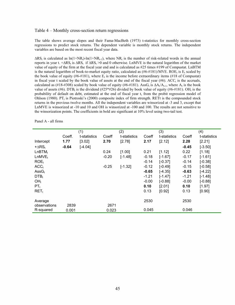
45

Table 4 – Monthly cross-section return regressions The table shows average slopes and their Fama-MacBeth (1973) t-statistics for monthly cross-section regressions to predict stock returns. The dependent variable is monthly stock returns. The independent variables are based on the most recent fiscal year data. ∆RSt is calculated as ln(1+NRt)-ln(1+NRt-1), where NRt is the number of risk-related words in the annual reports in year t. +∆RSt is ∆RSt if ∆RSt >0 and 0 otherwise. LnMVE is the natural logarithm of the market value of equity of the firm at the fiscal year end and is calculated as #25 times #199 of Compustat. LnBTM is the natural logarithm of book-to-market equity ratio, calculated as (#6-#181)/MVE. ROEt is Et scaled by the book value of equity (#6-#181), where Et is the income before extraordinary items (#18 of Compustat) in fiscal year t scaled by the book value of assets at the end of the fiscal year (#6). ACCt is the accruals, calculated as (#18-#308) scaled by book value of equity (#6-#181). AssGt is ∆At/At-1, where At is the book value of assets (#6). DTBt is the dividend (#25*#26) divided by book value of equity (#6-#181). OHt is the probability of default on debt, estimated at the end of fiscal year t, from the probit regression model of Ohlson (1980). PTt is Piotroski’s (2000) composite index of firm strength. RETt is the compounded stock returns in the previous twelve months. All the independent variables are winsorized at -3 and 3, except that LnMVE is winsorized at -10 and 10 and OH is winsorized at -100 and 100. The results are not sensitive to the winsorization points. The coefficients in bold are significant at 10% level using two-tail test. Panel A - all firms (1) (2) (3) (4) Coeff. t-statistics Coeff t-statistics Coeff t-statistics Coeff t-statistics Intercept 1.77 [3.02] 2.70 [2.78] 2.17 [2.12] 2.28 [2.21] +∆RSt -0.64 [-4.04] -0.45 [-3.50] LnBTMt 0.24 [1.00] 0.21 [1.12] 0.22 [1.18] LnMVEt -0.20 [-1.48] -0.18 [-1.67] -0.17 [-1.61] ROEt -0.14 [-0.37] -0.14 [-0.38] ACCt -0.25 [-1.32] -0.12 [-0.49] -0.15 [-0.58] AssGt -0.65 [-4.35] -0.63 [-4.22] DTBt -1.21 [-1.47] -1.21 [-1.48] OHt -0.00 [-0.88] -0.00 [-0.88] PTt 0.10 [2.01] 0.10 [1.97] RETt 0.13 [0.92] 0.13 [0.90] Average observations 2839 2671

2530 2530

R-squared 0.001 0.023 0.045 0.046

46

Panel B – positive ∆RS firms (1) (2) (3) (4) Coeff. t-statistics Coeff t-statistics Coeff t-statistics Coeff t-statistics Intercept 1.84 [3.03] 2.49 [2.54] 2.24 [2.11] 2.48 [2.31] ∆RSt -0.72 [-4.34] -0.60 [-4.06] LnBTMt 0.27 [1.10] 0.16 [0.80] 0.17 [0.88] LnMVEt -0.17 [-1.27] -0.19 [-1.66] -0.18 [-1.64] ROEt 0.05 [0.13] 0.03 [0.09] ACCt -0.39 [-1.64] -0.45 [-1.72] -0.48 [-1.85] AssGt -0.55 [-2.50] -0.51 [-2.28] DTBt -1.75 [-1.44] -1.81 [-1.50] OHt -0.00 [-1.92] -0.00 [-1.91] PTt 0.07 [1.27] 0.07 [1.32] RETt 0.11 [0.69] 0.10 [0.61] Average observations 1755 1653

1566 1566

R-squared 0.002 0.026 0.054 0.055

47

Table 5 – Equal-weight (EW) and value-weight (VW) returns of portfolios sorted on ∆RS Each month the ∆RS values of firms in the last fiscal year are used to allocate stocks to 11 portfolios. Firms with negative ∆RS are allocated to portfolio 0. Firms with positive ∆RS are allocated to portfolio 1 to 10, with portfolio 1 having the smallest increase in RS and portfolio 10 having the largest increase. The time-series mean and t-statistics are shown for both EW and VW portfolios. Two hedge portfolio returns are also shown. HGRET1 is the hedge portfolio formed by longing firms in portfolio 1 and shorting firms in portfolio 10. HGRET2 is the hedge portfolio formed by longing firms in portfolio 0 and shorting firms in portfolio 10. Excess returns are returns in excess of T-bill rate. The Alpha for each portfolio returns are the intercept in the regressions of the time-series portfolio excess returns of T-bill rate on the factor returns. The T-bill rate, the Fama-French three-factor and the momentum factor returns are from Kenneth French’s website. The numbers in bold are significant at 10% level using two-tail test. Panel A – EW returns (128 months)

Excess returns Alpha – three factor model

Alpha – four factor model

Mean t-statistics Coeff t-statistics Coeff t-statistics Ret0 1.37 [2.36] 0.37 [1.49] 0.74 [3.55] Ret1 1.52 [2.31] 0.47 [1.69] 0.82 [3.32] Ret2 1.65 [2.71] 0.64 [2.57] 1.03 [5.01] Ret3 1.26 [2.06] 0.27 [1.06] 0.63 [2.84] Ret4 1.46 [2.33] 0.38 [1.40] 0.83 [3.83] Ret5 1.32 [2.16] 0.29 [1.06] 0.73 [3.17] Ret6 1.02 [1.65] 0.05 [0.16] 0.51 [2.06] Ret7 1.30 [2.00] 0.27 [0.94] 0.75 [3.28] Ret8 0.85 [1.34] -0.18 [-0.59] 0.30 [1.20] Ret9 0.78 [1.33] -0.29 [-1.04] 0.21 [1.02] Ret10 0.60 [0.95] -0.52 [-1.67] -0.05 [-0.18] HGRET1 0.92 [3.35] 1.01 [3.62] 0.89 [3.14] HGRET2 0.77 [3.69] 0.94 [4.28] 0.83 [3.74]

Panel B – VW returns (128 months)

Excess returns Alpha – three factor model

Alpha – four factor model

Mean t-statistics Coeff t-statistics Coeff t-statistics Ret0 0.72 [1.48] -0.02 [-0.16] 0.04 [0.31] Ret1 1.55 [2.89] 0.82 [3.26] 0.78 [3.00] Ret2 1.00 [1.91] 0.24 [1.03] 0.26 [1.07] Ret3 0.45 [0.86] -0.27 [-1.13] -0.11 [-0.48] Ret4 0.71 [1.30] -0.14 [-0.49] 0.18 [0.67] Ret5 0.80 [1.68] 0.06 [0.27] 0.18 [0.79] Ret6 1.18 [2.20] 0.51 [2.09] 0.43 [1.75] Ret7 0.54 [0.93] -0.12 [-0.48] -0.13 [-0.51] Ret8 0.46 [0.80] -0.29 [-1.03] -0.18 [-0.63] Ret9 0.28 [0.53] -0.48 [-2.02] -0.34 [-1.44] Ret10 0.20 [0.37] -0.62 [-2.39] -0.49 [-1.88] HGRET1 1.34 [4.11] 1.43 [4.20] 1.26 [3.65] HGRET2 0.52 [2.00] 0.61 [2.24] 0.55 [1.95]

48

Table 6 - Additional tests The cross-section regressions (columns (1) and (2)) results show the average slopes and their Fama-MacBeth (1973) t-statistics for monthly cross-section regressions to predict stock returns. +∆RSt and ∆RSt are defined as in the notes for table 4. Column (1) use all sample firm-years. Column (2) uses only firm-years with positive ∆RSt. All the regressions also have the following control variables: LnMVE, LnBTM, ROE, ACC, AssG, DTB, OH, and PT, as defined in notes of table 4. All the variables in the cross-section regressions are winsorized at -3 and 3, except that LnMVE is winsorized at -10 and 10 and OH is winsorized at -100 and 100. The results are not sensitive to the winsorization points. The coefficients on the control variables are not shown. Columns (3) to (6) show the four-factor alpha’s of the returns of the equal-weight and value-weight hedge portfolios based on ∆RS. Each month the ∆RS values of firms in the most recent fiscal year are used to allocate stocks to 11 portfolios. Firms with negative RS are allocated to portfolio 0. Firms with positive RS are allocated to portfolio 1 to 10, with portfolio 1 having the smallest increase in RS and portfolio 10 having the largest increase. The time-series mean and t-statistics are shown for both EW and VW portfolios. Two hedge portfolio returns are also shown. HGRET1 is the hedge portfolio formed by longing firms in portfolio 1 and shorting firms in portfolio 10. HGRET2 is the hedge portfolio formed by longing firms in portfolio 0 and shorting firms in portfolio 10. The Alpha for each portfolio returns are the intercept in the regressions of the time-series portfolio excess returns of T-bill rate on the factor returns. The Fama-French three-factor, the momentum factor returns, and the T-bill rate are from Kenneth French’s website. Cross-section

regressions EW four-factor alpha VW four-factor alpha

(1) (2) (3) (4) (5) (6) +∆RSt ∆RSt HGRET1 HGRET2 HGRET1 HGRET2Pre-2000 years (56 months)

-0.51 [-3.34]

-0.70 [-3.80]

0.91 [2.03]

0.83 [2.49]

1.07 [1.96]

0.34 [0.84]

Post-2000 years (72 months)

-0.40 [-2.04]

-0.51 [-2.33]

0.73 [1.81]

0.72 [2.20]

0.74 [1.66]

0.23 [0.57]

Small firms (MVE<$150MM)

-0.51 [-2.50]

-0.69 [-2.58]

1.15 [3.10]

0.88 [2.90]

1.02 [2.63]

0.66 [2.26]

Big firms (MVE>=$150MM)

-0.39 [-2.47]

-0.45 [-2.51]

0.62 [1.94]

0.50 [1.94]

1.16 [3.22]

0.52 [1.82]

Price<$5 -0.47 [-1.49]

-0.76 [-1.93]

1.31 [2.21]

1.12 [2.31]

0.21 [0.22]

0.43 [0.58]

Price>=$5 -0.44 [-3.38]

-0.58 [-3.67]

0.73 [2.77]

0.55 [2.80]

1.23 [3.64]

0.53 [1.90]

Age<20 years -0.44 [-2.68]

-0.57 [-2.97]

0.57 [1.53]

0.69 [2.32]

1.53 [3.27]

1.07 [3.26]

Age>=20 years -0.28 [-1.86]

-0.54 [-3.02]

1.02 [3.75]

0.48 [2.12]

0.75 [1.69]

0.02 [0.04]

High growth industries (LTG>=20)

-0.76 [-2.73]

-0.81 [-2.70]

0.74 [1.54]

0.90 [2.90]

1.59 [2.11]

1.00 [1.51]

Low growth industries (LTG<20)

-0.35 [-2.12]

-0.44 [-2.30]

0.85 [2.53]

0.54 [2.15]

0.68 [1.54]

0.38 [1.16]

Form portfolios 3 months after filing date

-0.46 [-3.49]

-0.57 [-3.66]

0.65 [2.47]

0.66 [3.14]

0.78 [2.19]

0.28 [0.94]

Annual rebalancing on June 1

-0.41 [-3.05]

-0.47 [-3.40]

0.81 [3.16]

0.77 [3.81]

0.77 [2.28]

0.28 [0.97]

Firms with filing date in March only

-0.36 [2.08]

-0.44 [2.25]

0.78 [2.39]

0.60 [2.19]

1.62 [4.00]

0.46 [1.43]

49

Table 7 Control for stock return volatility Panel A shows the average slopes and their Fama-MacBeth (1973) t-statistics for monthly cross-section regressions to predict stock returns using the sample firm-years with positive ∆RS. ∆RSt, LnMVE, LnBTM, ROE, ACC, AssG, DTB, OH, and PT are defined as in the notes for table 4. IVOLm-1, calculated following Ang, Hodrick, Xing, and Zhang (2006) using daily stock returns, is the firm-specific idiosyncratic volatility relative to Fama-French three-factor model in the month prior to the return month. Panel B shows the excess return and four-factor alpha’s of the value-weight portfolios double sorted on ∆RS and IVOL independently using firms with positive ∆RS. Each month, firms are allocated into quintile portfolios based on the ∆RS values in the most recent fiscal year. Firms are also allocated into quintile portfolios based on IVOL of the most recent month. The time-series mean and t-statistics of the excess returns of the portfolios are shown. The column “(1-5)” refers to the difference in returns between portfolio 1 and portfolio 5. The Alpha for each portfolio returns are the intercept in the regressions of the time-series portfolio excess returns of T-bill rate on the factor returns. The Fama-French three-factor, the momentum factor returns, and the T-bill rate are from Kenneth French’s website. Panel A -- Monthly cross-sectional regressions of returns OLS Weighted LS

(weight=MVE)

Coeff. t-statistics Coeff. t-statistics Intercept 2.21 [3.22] 1.82 [1.70] ∆RSt -0.55 [-3.94] -0.62 [-2.02] LnBTMt 0.18 [1.03] 0.27 [1.17] LnMVEt -0.18 [-1.80] -0.03 [-0.28] ROEt 0.05 [0.17] 1.03 [2.37] ACCt -0.48 [-1.92] -1.18 [-3.16] AssGt -0.50 [-2.24] 0.07 [0.27] DTBt -1.57 [-1.38] -4.00 [-1.60] OHt 0.00 [-2.28] 0.00 [-0.76] PTt 0.07 [1.80] 0.02 [0.25] RETt 0.13 [0.86] 0.57 [2.43] IVOLm-1 1.09 [0.09] -13.40 [-0.81] Average observations 1565 1565 R-squared 0.069 0.181

50

Panel B – VW portfolios double sorted on IVOL and IVOL independently Ranking on ∆RS (1-5) Excess return 1 Low 2 3 4 5 High Return 4-factor Alpha

IVOL quintiles

Low 1 1.57 [3.31]

0.46 [0.92]

1.45 [2.86]

0.97 [2.00]

0.47 [0.95]

1.10 [2.10]

0.93 [1.71]

2 1.42 [2.33]

0.14 [0.20]

0.70 [1.09]

0.59 [0.82]

0.74 [1.24]

0.68 [1.41]

0.36 [0.73]

3 1.08 [1.15]

1.14 [1.48]

1.66 [2.02]

0.39 [0.48]

-0.40 [-0.50]

1.48 [2.54]

1.71 [2.60]

4 1.05 [0.92]

0.61 [0.61]

0.98 [1.05]

0.61 [0.58]

-0.24 [-0.22]

1.28 [1.71]

1.42 [1.66]

High 5 2.10 [1.59]

-0.59 [-0.49]

1.50 [1.09]

0.13 [0.10]

-0.74 [-0.53]

2.83 [3.33]

2.61 [3.18]

Panel C -- VW portfolios first sorted on IVOL and then on ∆RS within each IVOL quintile Ranking on ∆RS (1-5) Excess return 1 Low 2 3 4 5 High Return 4-factor Alpha

IVOL quintiles

Low 1 1.36 [2.80]

0.43 [0.86]

1.20 [2.48]

0.77 [1.56]

0.49 [1.06]

0.87 [1.66] 0.59 [1.14]

2 1.24 [1.97]

0.06 [0.08]

0.76 [1.17]

0.76 [1.07]

0.76 [1.25]

0.47 [1.00] 0.46 [0.86]

3 0.94 [1.02]

1.10 [1.37]

1.16 [1.48]

0.41 [0.52]

-0.59 [-0.75]

1.53 [2.51] 1.66 [2.59]

4 1.01 [0.90]

0.91 [0.88]

0.44 [0.45]

0.84 [0.77]

-0.55 [-0.52]

1.57 [2.41] 2.00 [2.54]

High 5 1.43 [1.14]

-0.11 [-0.11]

1.28 [0.98]

0.66 [0.52]

-1.43 [-0.99]

2.86 [3.74] 2.89 [3.76]

51

Table 8 – Analyst forecast and the information content of ∆RS Panel A shows the regressions of next year’s earnings change on risk sentiment and other variables that can predict future earnings, including analysts’ forecast of next year’s earnings. The dependent variable is ∆Et+1, calculated as Et+1-Et, where Et is the income before extraordinary items (#18 of Compustat) in fiscal year t scaled by the book value of assets at the end of the fiscal year (#6). ∆RSt is calculated as ln(1+NRt)-ln(1+NRt-1), where NRt is the number of risk-related words in the annual reports in year t. ∆Et is Et-Et-1. LnMVE is the natural logarithm of the market value of equity of the firm at the fiscal year end and is calculated as #25 times #199 of Compustat. LnBTM is the natural logarithm of book-to-market equity ratio, calculated as (#6-#181)/MVE. NegEt is a dummy that is 1 if Et is negative and 0 otherwise. ROEt is Et scaled by the book value of equity (#6-#181). –ACCt is accruals for firms with negative accruals (zero otherwise) and +ACCt is accruals for firms with positive accruals. Accruals is calculated as (#18-#308) scaled by book value of equity (#6-#181). AssGt is ∆At/At-1, where At is the book value of assets (#6). NoDt is a dummy that equals 1 if a firm has no dividend (0 otherwise). DTBt is the dividend (#25*#26) divided by book value of equity (#6-#181). OHt is the probability of default on debt, estimated at the end of fiscal year t, from the probit regression model of Ohlson (1980). PTt is Piotroski’s (2000) composite index of firm strength. All the variables are winsorized at -3 and 3, except that LnMVE is winsorized at -10 and 10 and OH is winsorized at -100 and 100. The results are not sensitive to the winsorization points. The regressions also include year fixed effects and two-digit SIC industry fixed effects and the coefficients are not shown. IFti is the mean IBES analysts’ forecast of year t+1 earnings in the ith month after the fiscal year t annual report filing date, scaled by book value of assets at the end of year t. The t-statistics in brackets are based on standard errors clustered by year. The coefficients in bold are significant at 10% level using two-tail test. Panel A: dependent variable -- ∆Et+1; sample – all firm-years with analyst forecast Coeff. t-statistics Coeff t-statistics Coeff t-statistics Coeff t-statistics Intercept -0.044 [-2.39] -0.038 [-2.22] -0.019 [-1.34] -0.007 [-1.34] ∆RSt -0.005 [-2.03] -0.005 [-2.11] -0.005 [-1.88] -0.004 [-1.30] ∆Et -0.043 [-2.98] -0.043 [-2.82] -0.047 [-3.19] -0.043 [-2.43] LnBTMt 0.011 [1.58] 0.008 [1.17] 0.002 [0.40] -0.000 [-0.08] LnMVEt 0.003 [1.51] 0.002 [0.80] -0.001 [-0.67] -0.003 [-1.71] NegEt -0.011 [-0.68] -0.002 [-0.12] 0.006 [0.36] 0.017 [0.93] ROEt -0.174 [-6.11] -0.190 [-6.27] -0.205 [-6.53] -0.205 [-6.30] -ACCt -0.098 [-2.58] -0.094 [-2.47] -0.077 [-2.22] -0.068 [-2.00] +ACCt -0.042 [-0.60] -0.006 [-0.12] -0.009 [-0.16] 0.006 [0.10] AssGt -0.035 [-8.31] -0.034 [-8.09] -0.035 [-8.71] -0.034 [-8.34] NoDt 0.000 [0.12] 0.000 [0.07] 0.001 [0.39] 0.001 [0.26] DTBt 0.108 [2.97] 0.106 [3.57] 0.121 [3.80] 0.117 [4.17] OHt 0.000 [0.10] -0.000 [-0.28] -0.000 [-1.10] -0.000 [-1.16] PTt 0.003 [1.90] 0.002 [1.51] 0.001 [0.70] 0.001 [0.61] IFt1 0.371 [8.84] IFt3 0.461 [10.85] IFt6 0.540 [18.49] IFt9 0.575 [18.63] Observations 17203 16730 16315 15933 R-squared 0.263 0.284 0.169 0.161

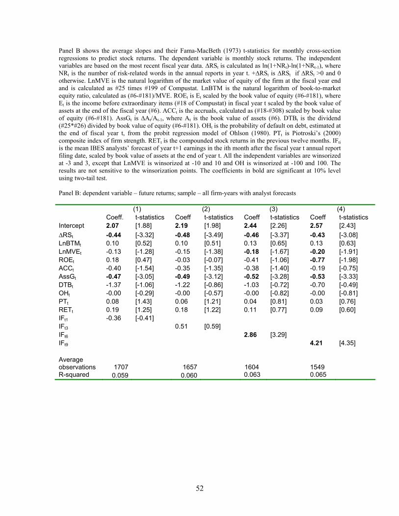
52

Panel B shows the average slopes and their Fama-MacBeth (1973) t-statistics for monthly cross-section regressions to predict stock returns. The dependent variable is monthly stock returns. The independent variables are based on the most recent fiscal year data. ∆RSt is calculated as ln(1+NRt)-ln(1+NRt-1), where NRt is the number of risk-related words in the annual reports in year t. +∆RSt is ∆RSt if ∆RSt >0 and 0 otherwise. LnMVE is the natural logarithm of the market value of equity of the firm at the fiscal year end and is calculated as #25 times #199 of Compustat. LnBTM is the natural logarithm of book-to-market equity ratio, calculated as (#6-#181)/MVE. ROEt is Et scaled by the book value of equity (#6-#181), where Et is the income before extraordinary items (#18 of Compustat) in fiscal year t scaled by the book value of assets at the end of the fiscal year (#6). ACCt is the accruals, calculated as (#18-#308) scaled by book value of equity (#6-#181). AssGt is ∆At/At-1, where At is the book value of assets (#6). DTBt is the dividend (#25*#26) divided by book value of equity (#6-#181). OHt is the probability of default on debt, estimated at the end of fiscal year t, from the probit regression model of Ohlson (1980). PTt is Piotroski’s (2000) composite index of firm strength. RETt is the compounded stock returns in the previous twelve months. IFti is the mean IBES analysts’ forecast of year t+1 earnings in the ith month after the fiscal year t annual report filing date, scaled by book value of assets at the end of year t. All the independent variables are winsorized at -3 and 3, except that LnMVE is winsorized at -10 and 10 and OH is winsorized at -100 and 100. The results are not sensitive to the winsorization points. The coefficients in bold are significant at 10% level using two-tail test. Panel B: dependent variable – future returns; sample – all firm-years with analyst forecasts (1) (2) (3) (4) Coeff. t-statistics Coeff t-statistics Coeff t-statistics Coeff t-statistics Intercept 2.07 [1.88] 2.19 [1.98] 2.44 [2.26] 2.57 [2.43] ∆RSt -0.44 [-3.32] -0.48 [-3.49] -0.46 [-3.37] -0.43 [-3.08] LnBTMt 0.10 [0.52] 0.10 [0.51] 0.13 [0.65] 0.13 [0.63] LnMVEt -0.13 [-1.28] -0.15 [-1.38] -0.18 [-1.67] -0.20 [-1.91] ROEt 0.18 [0.47] -0.03 [-0.07] -0.41 [-1.06] -0.77 [-1.98] ACCt -0.40 [-1.54] -0.35 [-1.35] -0.38 [-1.40] -0.19 [-0.75] AssGt -0.47 [-3.05] -0.49 [-3.12] -0.52 [-3.28] -0.53 [-3.33] DTBt -1.37 [-1.06] -1.22 [-0.86] -1.03 [-0.72] -0.70 [-0.49] OHt -0.00 [-0.29] -0.00 [-0.57] -0.00 [-0.82] -0.00 [-0.81] PTt 0.08 [1.43] 0.06 [1.21] 0.04 [0.81] 0.03 [0.76] RETt 0.19 [1.25] 0.18 [1.22] 0.11 [0.77] 0.09 [0.60] IFt1 -0.36 [-0.41] IFt3 0.51 [0.59] IFt6 2.86 [3.29] IFt9 4.21 [4.35] Average observations 1707 1657

1604

1549

R-squared 0.059 0.060 0.063 0.065

53

Figure 1 -- Value-weight hedge portfolio returns (HGRET1) by calendar year

-10

-5

0

5

10

15

20

25

30

35

1995 1996 1997 1998 1999 2000 2001 2002 2003 2004 2005

Year

Hedg

e po

rtfol

io r

etur

n (%

)

Note: This graph plots the annual compounded returns of the value-weighted portfolio HGRET1, as defined in Table 5.

Figure 2: Long-term growth rate revision

-1.8

-1.6

-1.4

-1.2

-1

-0.8

-0.6

-0.4

-0.2

01 3 6 9 12 15

Months after annual report file date

Cha

nge

in lo

ng-te

rm g

row

th

rate

Firms with ∆RS in the bottom 1/3 Firms with ∆RS in the middle 1/3 Firms with ∆RS in the top 1/3 Note: This graph plots the mean long-term growth rate revision made by IBES analysts in the 1 to 15 months after annual report filing date, relative to the forecasts made in the month before annual report filing date, for firms in the top 1/3, middle 1/3, and bottom 1/3 positive ∆RS portfolios.