Do Loan Officers Impact Lending Decisions?Evidence from the Corporate Loan Market*

Janet Gao Xiumin Martin Joseph Pacelli

Indiana University Washington University at St. Louis Indiana University

janetgao@indiana.edu xmartin@wustl.edu jpacelli@indiana.edu

March 14, 2017

Abstract

We examine and quantify the economic importance of loan officers in the corporate lending

process. We construct a comprehensive database that allows us to track the lending terms and

loan performance of corporate loans issued by over 7,000 loan officers employed by major U.S.

corporate lending departments during the period spanning from 1994 to 2012. We find that

loan officers have a substantial impact on both the contract terms (loan spreads, covenants,

and maturity) and the performance of corporate loans. The results are robust to controlling

for endogeneity concerns related to assortative matching in the labor market. Loan officers’

influence on the lending process has not declined much over time, despite technological inno-

vations designed to automate lending. Furthermore, these officers exhibit a greater impact on

the lending process in larger, more complex organizations in which information asymmetries

are more pronounced. Overall, our study sheds light on the inner workings of corporate bank-

ing departments and suggests that a significant portion of lending decisions are delegated to

individual loan officers.

Key words: Loan Officers, Human Capital, Syndicated Loans, Loan Contracts.

JEL classification: G30, G32, J24, D23

*We appreciate the helpful feedback and suggestions from workshop participants at Washington Univer-

sity at St. Louis, Greg Udell, and Robert Mahoney, the current CEO and president of Belmont Savings

Bank.

1 Introduction

A central objective of banks is to collect and process information (Petersen (2004)).

Accordingly, theoretical studies argue that banks, compared to bond investors, are su-

perior at producing information about their borrowers, especially when that information

is not publicly observable (Diamond (1984, 1991), Ramakrishnan and Thakor (1984)).

Rapid consolidation in the banking industry coupled with technological advancements

have potentially reshaped the information production processes underlying many lending

decisions (Petersen and Rajan (2002)). Within these modern organizations, loan officers

at lower tiers are typically responsible for collecting information about borrowers and

transmitting this information to managers of the bank (Stein (2002)). However, with the

existence of multiple layers and advanced technology within a bank, it is not clear where

the final decision rights reside between the headquarters and loan officers.

In this study, we examine and quantify the relative importance of individual loan

officers compared to their institutions in setting loan terms and influencing loan perfor-

mance. Our goal is to shed light on how information is produced and used in banks’

lending decisions. Ultimately, banks face a trade-off between complete delegation, where

lower-tiered agents (such as loan officers) make final lending decisions, and centralization,

where decision rights are concentrated completely at headquarters. Too much delegation

could lead to information manipulation due to loan officers having misaligned incentives

and facing costly communication (Stein (2002), Dessein (2002), Agarwal and Hauswald

(2010), Gropp et al. (2012), Brown et al. (2012)), while too little delegation could result

in the loss of valuable soft information regarding the banks’ borrowers. With improve-

ments in lending technology and financial reporting quality, recent research suggests that

banks may be able to rely more on hard information (Petersen and Rajan (2002), Berger

et al. (2005)). As such, it remains unknown how much decision rights are delegated to

loans officers. This study seeks to bridge this gap by piercing the “black box” of banks’

corporate lending activities.

We focus on the market for corporate loans, as it represents an important source

of financing for corporations and a major service provided by banks (Roberts (2015)).

1

Moreover, corporate lending contains significant information asymmetries between banks

and their borrowers, thus providing a setting in which loan officers’ judgment may be

a valuable asset for banks. Traditionally, data on the identities of loan officers issuing

corporate loans are not readily available, making it difficult for researchers to distinguish

the effect of the loan officer on the lending process from that of the bank. To overcome

this data challenge, we collect and analyze 4,215 loan agreements from SEC filings in

which we identify the loan officers underwriting these contracts. We then supplement

these SEC documents using loan contract terms provided by LPC Dealscan. To our

knowledge, this represents one of the most comprehensive databases on U.S. loan officer

employment as it contains 7,892 loan officers working in major U.S. corporate lending

departments from 1994 to 2012. These officers issue nearly $1.8 trillion in financing to

1,678 corporate borrowers over our sample period. Importantly, our dataset allows us

to observe loan officers at different points of employment over their careers and to track

the lending terms and loan performance related to a particular loan officer as she moves

across banks.

Our objective is to identify and quantify the effects of loan officers in the lending

process. To this end, we exploit loan officer turnover as an important source of varia-

tion to estimate loan officer fixed effects. We employ empirical methods developed by

Abowd, Kramarz, and Margolis (1999) and Abowd, Creecy, and Kramarz (1999) that

allow the estimation of individual effects in large panel data (hereafter, AKM method).

This methodology identifies bank fixed effects using changes in lending outcomes asso-

ciated with loan officers moving between banks, and identifies loan officer fixed effects

by removing the estimated bank fixed effects from individual loan outcomes. Following

recent research distinguishing the effects of institutions and individuals in labor market

settings (e.g., Graham et al. (2012), Ewens and Rhodes-Kropf (2015), Liu et al. (2016)),

we adopt this methodology to quantify the extent to which loan officers influence lending

processes within corporate lenders.

Our analyses reveal an economically important role of loan officers in the lending pro-

cess. We first estimate loan officers’ impact on three common lending terms: loan spread,

2

loan covenant, and loan maturity. We find that loan officers explain a substantial portion

of the variation in lending terms. For example, loan officer effects explain approximately

24% of the variation in loan spreads. Relatively speaking, loan officer effects explain

about five times as much variation in loan spreads as do bank fixed effects. These results

suggest that loan officer fixed effects are economically significant in both an absolute and

relative sense. Similarly, loan officers explain five times more variation in loan covenants

and nine times more variation in loan maturity than do banks. These findings are robust

to controlling for observable characteristics of the borrower and loan contracts. This ini-

tial analysis thus suggests an important role of loan officers in setting corporate lending

terms.

As loan officers are delegated with significant power in designing loan contract terms,

it is natural to conjecture that their influence will have implications for future loan per-

formance. Therefore, our next set of analyses examines loan officers’ effects on loan

performance, as measured by future borrower defaults, downgrades, and accounting per-

formance (i.e., ROA). The evidence from these tests confirms this conjecture. For ex-

ample, our estimates suggest that loan officer fixed effects explain 47% of the variation

in future borrower default, which is much greater than the variation explained by other

borrower and loan characteristics combined. In addition, loan officers explain over 13

times more variation in the occurrence of defaults in loan portfolios than do banks alone.

We generate similar inferences using other measures of performance. Taken together, the

evidence from our main analyses suggests that loan officers play an important role in

both setting lending terms and influencing loan performance.

Before proceeding, it is critical to note that the estimation techniques we employ

rely on non-random loan officer movement, and that these methods can admit potential

endogeneity concerns. Indeed, these concerns represent a limitation common to all studies

relying on employee movement as a source of variation (Graham et al. (2012), Ewens and

Rhodes-Kropf (2015), Liu et al. (2016)). Outside of experimental settings, it is difficult

to perfectly isolate employee effects due to the scarcity of exogenous movement. Research

must inevitably face a trade-off between the loss of precision available in experimental

3

settings, and the gains associated with generalizable, large-scale evidence of economic

phenomena. We view our study as a complement to prior experimental research on loan

officers’ behavior (e.g., Liberti and Mian (2009), Agarwal and Ben-David (2014)). We

extend this line of research by quantifying the effects of loan officers in an important

lending market across a long time span and a wide-spectrum of banks. At the same time,

we are cognizant of the limitations of our analysis. We conduct a battery of robustness

tests to address these concerns in turn.

First, we address a common issue associated with the AKM methodology in that

individual fixed effects may be over-estimated when we only observe limited movement

in the sample. With movers comprising 17% of our sample, our data structure is unlikely

to introduce significant biases in our findings.1 Nevertheless, we re-examine our analysis

by restricting our sample to only movers (i.e., loan officers that can be observed in at

least two banks during the sample period). Using this subsample, we directly compare

the incremental R2 attributed to loan officer fixed effects and bank fixed effects.2 Even

in this subsample restricted to movers, loan officers explain at least two to three times

more variation in lending terms and loan performance than do bank fixed effects. This

suggests that our inferences are unlikely to be biased by limited movement.

We next examine whether and to what extent assortative matching between loan

officers and banks affects our findings (Becker (1973)). Assortative matching entails

banks’ tendency to hire loan officers with similar quality, risk preferences, or judgment.

It is important to note that assortative matching does not always pose a challenge to our

inferences as it often will result in loan officer fixed effects being under-estimated in the

AKM framework. For example, if movement is a result of loan officers seeking positions

in banks that have similar time-invariant characteristics related to their lending decisions

(e.g., risk tolerance), the AKM method would over-estimate the bank’s effect, which biases

against our conclusion that loan officers matter in the lending process. Accordingly, we

conduct detailed analyses and focus our attention on scenarios in which bank effects are

1This figure is also in line with prior studies using the AKM method (e.g., Graham et al. (2010),Ewens and Rhodes-Kropf (2015)).

2This method is commonly referred to as the mover-dummy-variable method (MDV).

4

likely under-estimated.

We begin by visually inspecting the severity of assortative matching in the data. To

do so, we compute the variation in loan contract terms extended by all loan officers in

a given bank-year, and compare this with the variation in loan contract terms generated

by a randomly-selected, equal-sized group of loan officers employed across all banks in

the same year. Our visual inspection of the variances suggests that assortative matching,

although present, is not pronounced in our data. In some scenarios, the variation in loan

contract terms extended by loan officers in our sample is almost indistinguishable from

those generated by a randomly-selected group of loan officers.

Next, we examine whether time-varying lending policies across banks influence our

findings. For example, a bank may change its lending policies over time and hire loan

officers that are aligned with this new direction. This represents a concern because the

movers we observe (i.e., newly hired loan officers) may exhibit similar lending preferences

prior to the move as the lending policies at the bank of interest. In this case, one

would under-estimate time-invariant bank effects using the AKM method. Accordingly,

we control for banks’ time-varying lending policies by including bank-year fixed effects

in our baseline framework. Our findings continue to indicate that loan officers explain

a large portion of the variation in lending terms and loan performance. This test also

represents an important extension from prior studies examining individual fixed effects,

as these studies generally do not have sufficient variation to control for time-varying

preferences of the employer (e.g., Graham et al. (2012)).

We further consider scenarios in which we only observe movers between similar banks.

Bank effects will be under-estimated in such scenarios since the original bank and des-

tination bank of a given mover have similar lending policies. To alleviate this concern,

we re-examine our analyses using a subsample of banks connected by loan officers that

move to different categories of banks in terms of market share rankings (i.e., moving up

or moving down in bank ranking). Our inferences remain unchanged in this subsample.

Finally, we consider additional matching concerns related to loan officers’ selection of

borrowers. Conceptually, we do not exclude the choice of borrowers from loan officers’

5

lending decisions. Nonetheless, to better understand whether loan officers’ choice of

borrower influences our findings, we conduct an additional analysis that purges the choice

of borrower from loan officers’ lending decisions. To do so, we modify our baseline models

by controlling for bank-firm pairings, which artificially attributes all the decision rights in

borrower selection to banks. Our results continue to hold in this analysis, indicating that

the non-random assignment of borrowers to loan officers does not explain our findings.

Overall, the battery of robustness tests we conduct verifies our baseline findings that

loan officers play an important role in setting lending terms and influencing loan per-

formance. Similar to prior studies, we recognize that the complexity of labor market

matching creates endogeneity problems that cannot be completely addressed (Graham et

al. (2012), Ewens and Rhodes-Kropf (2015)). Importantly, our tests offer several novel

extensions to the prior literature. For example, by controlling for bank-year two-way in-

teractive effects, we can alleviate to a large extent concerns regarding time-varying bank

characteristics influencing our findings.

Our next analyses examine cross-sectional and time-series variation in the explana-

tory power of loan officer fixed effects. We first partition banks by the size and industry

concentration of their loan portfolios, and find that loan officers explain a greater por-

tion of the variation in lending terms and loan outcomes in banks with larger and more

diverse loan portfolios. These findings suggest that complex organizations might benefit

more from delegation, potentially due to the increased communication costs associated

with transmitting soft information through organizational hierarchies and greater risks of

information manipulation in that process. We next partition our sample into four time

periods of similar sample size to investigate whether technological improvements have

reduced banks’ dependence on loan officers collecting soft information in the lending pro-

cess (Rajan and Petersen (2002), Berger et al. (2005)). Loan officer effects explain a

large portion of the variation in lending terms and loan performance across all subsam-

ples, suggesting that either the corporate lending process is difficult to automate or the

automation process continues to involve significant human judgment. Interestingly, we

find that loan officers have a substantial effect on loan performance in the pre-crises years,

6

consistent with the argument that agency problems were intensified prior to the crises.

Finally, having established evidence that loan officers play an important role in the

corporate lending process, we conduct exploratory analyses to further understand the

inter-relations and sources of loan officers’ fixed effects. First, we correlate estimated

loan officer fixed effects across different lending terms and loan performance to identify

whether there are overarching patterns in loan officers’ lending decisions. We find that

loan officers who include more covenants in loan contracts tend to charge lower interest

rates and shorten debt maturity. Officers also seem to pair high interest rates with long

maturities. Importantly, we find that officers who consistently impose higher interest rates

tend to issue riskier loans. These results suggest certain strategies in lending decisions.

We further investigate whether loan officers’ personal backgrounds contribute to this

heterogeneity. We collect information regarding loan officers’ educational background,

gender, and place of first employment from LinkedIn. We find evidence suggesting that

loan officers who studied at top tier schools tend to charge higher interest rates. In

addition, officers that begin their career at large institutions are more likely to originate

loans with short maturity and issue loans that perform poorly. However, these observable

characteristics only explain a negligible portion of the variation in their lending decisions,

suggesting that these decisions are likely attributable to other, unobservable factors.

Our study contributes to the literature in several ways. First, we provide the first

large-sample evidence showing the role of individual loan officers in the corporate lending

process. There is a burgeoning literature examining the role of loan officers and how

they respond to various incentive schemes (e.g., Liberti and Mian (2009), Berg, Puri,

and Rocholl (2013), Mosk (2014), Drexler and Schoar (2014), Degryse et al. (2014),

Agarwal and Ben-David (2014), Cole et al. (2015), Karolyi (2017)).3 However, these

studies generally sample on foreign lending markets, different banking products, or focus

on experimental settings inside a single bank. Our broad sample of loan officers enables us

to examine and quantify the importance of loan officers in the corporate lending market.

3In a related study, Herpfer (2016) examines the role of soft information in lending relationships. Hisstudy focuses on the role of time-varying soft information and examines a smaller sample of loan officersemployed primarily by lead banks.

7

Our finding that loan officers consistently play a significant role in the lending process over

time complements studies that document changes in banks’ reliance on soft information

(Petersen and Rajan (2002), Berger and Udell (2004)).

Second, we contribute to a growing literature examining the relative importance of

employees within a firm (e.g., Bertrand and Schoar (2003), Schoar and Zuo (2017), Gra-

ham, Li and Qiu (2012), Ewens and Rhodes-Kropf (2015), Liu et al. (2016)). These

studies generally suggest that executives, fund partners, and inventors have significant

influence over corporate decisions and performance. Our study contributes to this liter-

ature in two dimensions. First, our study is among the first to highlight the influence

of lower-level employees inside large organizations, such as loan officers. Second, we fo-

cus on the function of those employees in financial intermediaries (Petersen 2004). The

heterogeneity in the influence of loan officers we document reflects the varying degree of

delegation across banks in the corporate lending market.

Finally, our study extends the literature examining corporate loan markets, in par-

ticular, studies documenting persistent lender characteristics affecting loan performance

and contract terms (Billet, Flannery and Garfinkel (1995), Ross (2010), Gopalan, Nanda

and Yerramilli (2011), Bushman and Wittenberg-Moerman (2012), Ellull and Yerramilli

(2012)). Complementary to these studies, our study quantifies the explanatory power of

the time-invariant dimension of loan officers’ heterogeneities and compares that with the

banks where these loan officers are employed. The main takeaway is that loan officers

appear to play an economically meaningful role in the syndicated lending market.

This paper develops as follows: Section 2 describes our data source, variable construc-

tion, and empirical methodology. Section 3 describes the univariate patterns of our data.

Section 4 provides our main results. Section 5 discusses and addresses the endogeneity

concerns related to our findings. Section 6 exploits cross-sectional variation. Section 7

concludes.

8

2 Data & Empirical Methodology

2.1 Sample Selection

We begin our sample selection by retaining all loans issued on LPC Dealscan between

the years 1994 and 2012. We start with a sample of 93,073 loans with information

regarding contract terms, including spreads, covenants, and maturity. To be included in

the sample, we require borrowers to have available financial information from Compustat.

We further exclude borrowers in financial and utility industries as they generally have less

comparable financial policies. This procedure leaves us with an initial sample of 41,977

loans extended to 4,446 firms.

2.2 SEC Filings

Based on the initial Dealscan sample, we search SEC filings for the official contracts

related to these loans. Loan contracts are considered material public disclosures and are

generally filed as Exhibits to firms’ 8-K’s, 10-Q’s and 10-K’s. In particular, we search

for any public filing that contains an appended Exhibit 10 (which relates to “Material

Contracts”). We further require the contract to contain either the word “loan” or “credit”

followed by “agreement” in the title to ensure that the material contract we are extracting

relates to a loan agreement, as opposed to other contracts (e.g., supply agreements,

executive compensation agreements, etc.). We search for all filings meeting this criteria

in the 90-day window centered on the loan initiation date observed in Dealscan. Doing

so allows us to account for errors in the dates that Dealscan reports.4

A large proportion of loan agreements contain signature pages attached to the end

of the agreement. These signature pages allow us to identify the names of loan officers.

Accordingly, we require the documents in our sample to contain the string “/s/”, which

indicates that the document contains such a signature page. Following this symbol, we

extract the name of the loan officer, the bank in which she is employed, and her title as

shown in the signature page. This process results in a sample of 7,892 unique loan officers

4As noted in Murfin (2012), Dealscan sometimes reports loan dates at a lag due to delays related tobanks approving term sheets and receiving mandates.

9

with 4,215 loan contracts, representing a 10% match to the original loan sample. While

this sample may seem small, it is important to note that the SEC Edgar database was

not complete for our entire sample period.

Before proceeding, it is important to discuss some assumptions and judgments we

have to make with respect to our data collection process. First, we assume that loan

officers who signed the loan contracts appended to SEC documents are the loan officers

responsible for screening and monitoring the borrower. Per our discussion with an in-

dustry practitioner, syndicated loans are commonly written and monitored by a team

consisting of a managing director or senior vice president, a loan officer and a credit

analyst at each lead bank and participant bank. The managing director or senior vice

president usually supervises the whole syndication team. The majority of loan officers in

our sample have a title of “Vice President” (Figure 1). We therefore believe it is appro-

priate to attribute loan performance to these officers as they likely had some influence

in the lending decision. Second, we identify loan officer turnovers by the dates and the

affiliation listed on the loan contracts. We admit that this identification is imprecise. As

such, we do not observe the exact timing that a loan officer transition between banks in

her career. However, this limitation does not affect our empirical inferences because our

unit of analysis is at the loan-bank-officer level.

2.3 Variables of Interest

2.3.1 Loan Terms

We examine three aspects of loan contract terms that prior studies consider to be im-

portant dimensions of the debt contracting process (e.g., Bharath et al. 2011, Chava and

Roberts 2008). We first consider interest rate spreads (Loan Spreads), representing the

markup charged by the lender (all-in-drawn spreads, in basis points over LIBOR). Next,

we examine the total number of covenants included in a loan package (Loan Covenants).

We also consider the maturity of the loan contract (Loan Maturity), measured as the

number of months until the loan matures. These terms encompass both the pricing and

non-pricing dimensions of a loan contract.

10

2.3.2 Loan Performance

We also examine three measures of loan performance. Our main measure is the

occurrence of default. We define an indicator variable Default that takes the value of one

if a borrower receives a default rating as per S&P (“D” or “SD”) or files for bankruptcy

before the loan matures, and zero otherwise. Albeit rare, defaults constitute the most

extreme credit events that can occur in a lending portfolio. We thus use Default as

the primary measure of loan performance. We also construct a supplementary, yet less

extreme measure of loan performance: the extent of borrowers’ downgrades (Downgrade).

To construct this measure, we decode all S&P ratings from (AAA = 1, AA+ = 2,..., and

D or SD = 22), and calculate the difference in ratings for the borrower from the loan

initiation date to loan maturity. Downgrades suggest that borrowers are less likely to

meet their debt obligations. Our final measure of loan performance is borrowers’ average

profitability over the course of the loan (ROA). Although it does not represent direct

losses to lenders, borrowers’ ROA provides a continuous metric that can reflect declines

in future credit quality (Bushman and Wittenberg-Moerman (2011)).

2.3.3 Control Variables

We include control variables related to characteristics of the borrower and the loan

contract (defined in Appendix A). Firm controls include Size, Age, Profitability, Tangi-

bility, M/B, Leverage, and an indicator for whether a firm receives credit ratings (Rated).

Loan controls include Loan Spreads, Loan Covenants and Loan Maturity when they are

not examined as outcome variables. We also control for Loan Size, an indicator for

whether the bank is a Lead Arranger, and loan type fixed effects (e.g., revolver, term

loan A, term loan B, etc.). The models also include year and borrower industry fixed

effects. We winsorize all continuous variables except leverage to 5th and 95th percentiles.

We restrict Leverage to be within 0 and 1. Detailed definitions of these variables are

described in Appendix A.

11

2.4 Loan Officer Fixed Effects Models

Our research objective is to disentangle the effects of loan officers from those of banks

in the lending process. In this section, we outline the fixed effects methodology we employ.

We begin with a baseline model that regresses lending terms and loan performance on

firm characteristics, loan terms (other than the dependent variable), borrower-industry

fixed effects, and year fixed effects:

Yibkt = β1Xjt + β2Zk + δh + µt + εibkt, (1)

where i denotes loan officer, b denotes bank, j denotes the firm in which the loan officer

lends to, k denotes the loan package, and t denotes time. In the above equation, Yibkt is

either the lending term (Spread, Covenants, or Maturity) or loan performance (Defaults,

Downgrades, or ROA) associated with loan officer i’s loan to firm j at time t while

employed by bank b. The variables Xjt and Zk control for time-varying attributes of

the borrower and loan contracts, as discussed in Section 2.3.3. The vector δh captures

industry-fixed effects for which firm j is a member of. The vector µt controls for year

fixed effects.

To estimate the explanatory power of individual loan officers and the banks that

employ them, we next add loan officer- and bank-fixed effects φi and θb to Eq. 1:

Yibkt = β1Xjt + β2Zk + δh + µt + φi + θb + εibkt, (2)

Our objective in this analysis is to retrieve the loan officer- and bank-fixed effects φi

and θb by exploiting variation in loan officers employed at the banks in our sample, and

estimate their incremental explanatory power to the variables of interest.

In order to estimate loan officer fixed effects from Eq. 2, one needs to observe loan

officer movement. As such, a loan officer must be observed in at least two banks in

the sample, and a bank must employ at least two such loan officers. This empirical

approach was originally presented in Bertrand and Schoar (2003) and has subsequently

been referred to as the mover dummy variable approach (MDV). One concern with this

12

approach is that it relies on a sample consisting of only movers, thus potentially limiting

the external validity of the analysis. Accordingly, our main analysis relies on a modified

version of the MDV approach introduced by Abowd, Kramarz, and Margolis (1999) and

later refined by Abowd, Creecy, and Kramartz (2002), henceforth the AKM method.

The AKM method allows us to expand our analysis to both “movers” and “non-

movers.” With the AKM method, we are able to separate loan officer and bank fixed

effects through a connectedness sample containing a set of banks connected through

movers. To construct the connectedness sample, we track all the banks that loan officers

in our sample are ever employed by, and consider a common loan officer as a “connection”

between banks. Using these connections, we extract all the connected components as our

sample of banks, thus requiring all banks to employ at least one loan officer that can be

observed in another bank. This allows us to estimate loan officer and bank fixed effects

within the connected set of banks following the procedures outlined in Cornelissen (2008)

and more recently, Liu et al. (2016).

The following steps illustrate the AKM approach in more detail. We begin by mod-

ifying Eq. 2 to allow for the estimation of loan officer and bank effects through the

connectedness sample as opposed to the “movers” only sample. As discussed above, this

approach includes all loan officers and banks regardless of whether the loan officer tran-

sitions across banks. To illustrate, consider the dummy variable Dibt which is equal to

one if loan officer i works at bank b in year t and zero otherwise. Eq. 2 can be rewritten

as follows:

Yibkt = β1Xjt + β2Zk + δh + µt + φi +B∑b=1

Dibtθb + εibkt, (3)

where J indicates the collection of banks in our sample.

The AKM method first averages across all of loan officer i’s lending terms or loan

performance outcomes to obtain the following:

Yi = β1Xi + β2Zi + δi + φi +B∑b=1

Dibθb + µt + εi, (4)

Accordingly, Yi is the average lending term or loan performance for a deal associated with

13

a loan officer across the entire sample period. Next, Eq. 3 can be demeaned by Eq. 4:

(Yibkt−Yi) = β1(Xjt−Xi)+β2(Zt−Zi)+(δh− δi)+c∑

b=1

(Dibt−Dib)θb+(µt−µt)+(εibkt− εi),

(5)

The demeaning process removes the loan officer fixed effects (φi) from the estimation

process. Accordingly, we are able to use movers’ information to identify bank fixed effects

since Dibt − Dib 6= 0 for a mover. This can be estimated using the least square dummy

variable approach following Andrews et al. (2006). We can then re-arrange the terms in

Eq. 4 to obtain the following estimates of loan officer fixed effects:

φi = Yi − β1Xi − β2Zi − δi −B∑b=1

Dibθb − µt (6)

It is important to note that prior studies indicate that an estimation bias might result

if our loan officer movement sample is small (Abowd et al. (2004), Andrews et al. (2006),

Liu et al. (2016)). We do not expect this bias to be severe in our sample as we observe

about 17% of loan officers move across banks in our connectedness sample. This number

is similar to recent studies using the AKM procedure.5

In sum, we view both the AKM and MDV approaches as having trade-offs. The AKM

method allows us to infer connections through the full sample of loan officer and bank

pairs and thus is more generalizable.6 However, this method also introduces potential

biases if the sample of movers is small. On the other hand, the MDV approach focuses

on only movers and reduces the potential for such biases to arise, but is limited in its

external validity. Consistent with prior literature, we present the AKM method as our

primary analysis, and demonstrate the robustness of our results using the mobility sample

and the MDV approach.

5For example, Liu, Mao, and Tian (2016) report that 16% of inventors in their sample move, Ewensand Rhodes-Kropf (2015) report 30% of venture capital partners move in their sample, and Graham, Li,and Qiu (2012) report that only 5% of executives in their sample move.

6Note that prior studies also indicate that the AKM method has the added benefit of being morecomputationally feasible. However, we refrain from making this claim for our sample given the substantialincreases in computing power in recent years. For example, Graham, Li, and Qiu (2012) claim thatapproximately 6GB of memory is needed to compute MDV fixed effects for a sample of 65,000 executives.This amount of memory is rather standard in current computer configurations.

14

3 Univariate Analyses

3.1 Loan Officer Descriptive Statistics

Table 1 describes the movement of loan officers in our sample. Panel A presents the

frequency of loan officers moving within our sample. Our final sample consists of 7,892

loan officers, of which 1,325 move at least once during our sample. Thus, movers represent

nearly 17% of our sample. This statistic is comparable to recent studies examining

employment movement. For example, Graham et al. (2012) and Liu et al. (2016)

find that movers account for approximately 5% and 16% of the population of employees

examined, respectively. Panel B reports the number of banks with movers. Our sample

consists of 982 banks, of which about 55% employ at least one mover during the sample

period. Moreover, 42% of banks in our sample employ between one to five movers. As we

examine higher thresholds on the number of moves per bank (e.g., 6–10, 11–20, etc.), we

find that these banks constitute less of our sample. Consistent with prior studies, there is

a negative relation between the number of banks and the number of movers they employ.

Table 1 About Here

Figure 1 reports the distribution of the titles for loan officers in our sample, as observed

in the electronic signatures extracted from the SEC loan contracts. Roughly 60-70% of

loan officers in our sample hold positions as senior vice presidents (Senior VP), vice pres-

idents (VPs) or managing directors. About 10-15% of loan officers are bank CEOs and

board directors. As our study focuses on mid-level managers, we conduct robustness

analyses (untabulated) excluding these senior employees. All our results are both qual-

itatively and quantitatively similar when we exclude higher-level management from the

sample.

Overall, the trends in Table 1 indicate that the labor market for loan officers appears

to be quite dynamic. We document substantial variation in both the number of banks in

which loan officers are employed as well as the number of moves each bank experiences.

This variation suggests that we can exploit fixed effects models in separating the effects

15

0

0.05

0.1

0.15

0.2

0.25

0.3

0.35

0.4

0.45

0.5

Chief Executives Managing

Directors

Senior VP VPs Associate and

Analysts

Other

Percentage of Officers by Title

Leader Participants

Figure 1. Distribution of loan officer titlesThis figure describes the distribution of the titles of loan officers that issued syndicated loan contracts.The vertical axis represents the percentage of total loan officers. The horizontal axis displays titles in abank. The solid columns indicate the percentage of officers with each title in a syndicated lead arrangerbank. The patterned columns indicate the percentage of officers in a participant bank.

of loan officers and banks in lending decisions.

We further visualize the career movement of loan officers using a group of banks across

which we observe at least 20 movers. Figure 2 describes the mapping among this set of

banks. In this plot, the size of each node is proportional to the number of movers within

each bank. The edges connecting the nodes represent the connections among banks that

are formed by movers. Bank of America Merill Lynch, Wells Fargo, and JP Morgan are

among the top in terms of officer movements. This is consistent with prior empirical

evidence indicating that these banks also dominate the syndicated lending market in

terms of market share (Ross (2010)).

We next inspect the number of loans issued by each loan officer as observed in our

sample. This helps us better understand the data structure and validate the testing

sample. Figure 3 counts the number of loans issued by each loan officer in our sample,

and plots the percentage of loan officers observed issuing a given number of loans. Over

70% of loan officers in our sample issue fewer than three loans, and 44% of them issue

only one loan.

With this data structure, we continue to examine whether loan officers in our sample

specialize in extending credit to certain industries. Using the industry classification of

16

●

●

●

●

●

●

●

●

●

●

●

●

AIB

Fifth Third

SunTrust

Wells Fargo

PNC

US Bancorp

Comerica

Northern Trust

GE Capital

Goldman Sachs

TD

Credit Suisse

Societe Generale

Deutsche

RBS

HSBC

KeyBank

UBS

ING

BBVA

BNPJP Morgan

Mizuho

Morgan Stanley

RBC

Mitsubishi

BMO

Citi

BNY MellonLloyds

BOA

Sumitomo

Credit Agricole

Barclays

Scotiabank

Figure 2. A network of banks connected by officer movementThis figure describes the connectedness among a set of banks that contain at least 20 movers (officersthat can be observed in more than one banks). The size of the nodes reflects the number of moverswithin the sample of banks.

our sample borrowers, we count the number of industries covered by a given loan officer

and plot the distribution of loan officers covering a certain number of industries. Figure 4

describes the industry concentration of loan officers. The majority of loan officers issue

loans in only one industry, and nearly 90% of loan officers issue loans in only one or

two industries.7 This pattern suggests that the job function of loan officers is highly

specialized.

Finally, we examine whether our sample fairly represents the Dealscan universe, as

there is a high level of attrition when we match Dealscan data to SEC documents. Accord-

ingly, Figure 5 compares the industry distribution of borrowers in the Dealscan universe

to the industry distribution of borrowers in our sample. The figures suggest that the ma-

7As shown in Figure 3, single loan officers (i.e., loan officers issuing only one loan) represent 30 percentof our sample. Therefore, the observed industry concentration of loan officers are unlikely to be drivenby officers with only one loan.

17

0%

5%

10%

15%

20%

25%

30%

35%

40%

45%

50%

1 2 3 4 5 6 7 8 9 10 >10

Per

cen

tage

of

Loan

Off

icer

s

Number of Loans Issued

Figure 3. Number of loans issued by a loan officerThis figure describes the number of loans issued by a given loan officer. The horizontal axis shows thenumebr of loans issued by a loan officer, and the vertical axis suggests the percentage of officers issuingthe corresponding number of loans.

jority of borrowers in both samples are concentrated in manufacturing industries. The

percentage of borrowers in other industries is also similar: Transportation & Communi-

cation, Services, Wholesale & Retail, and Mining industries constitute the majority of

borrowers outside of manufacturing industries. Agricultural firms, on the other hand,

constitute a very small portion of the sample. Overall, the visual inspection of industry

composition suggests that the sample attrition does not affect the generalizabilty of our

inferences to the entire Dealscan universe of borrowers.

3.2 Summary Statistics

Table 2 describes the summary statistics of our variables of interest. For each variable,

we report the statistics from four samples. We start with the initial sample from Dealscan

that we match to borrowers’ SEC filings. This sample contains 41,977 loan contracts,

24,693 of which have complete information regarding loan contract terms and borrower

characteristics. After matching the initial Dealscan sample with loan officer signature

data from SEC documents, we are left with a sample of 15,513 loan contract-officer

observations (“Full Sample”) in which we observe all borrower characteristics. To conduct

AKM analyses, we further restrict the full sample to the loan contracts extended by

a group of banks that are connected by movers (“Connectedness Sample”). Finally,

18

0%

10%

20%

30%

40%

50%

60%

70%

80%

1 2 3 4 5 6 7 >7

Per

cen

tage

of

Lo

an O

ffic

ers

Number of Industries Covered

Figure 4. Industry coverage of loan officersThis figure describes the number of industries covered by a given loan officer inside a bank. Industry isdefined by two-digit SIC industries. The horizontal axis indicates the number of industries covered by aloan officer, and the vertical axis suggests the percentage of officers covering the corresponding numberof industries.

Agriculture

Mining

Manufacturing

Transportaion & Communication

Wholesale & Retail

Services

(a) Distribution of Borrower Industry in Dealscan

Agriculture

Mining

Manufacturing

Transportation & Communication

Wholesale & Retail

Services

(b) Distribution of Borrower Industry in Sample

Figure 5. Distribution of Borrower Industries. This figure presents the percentage of borrowers’industries in all Dealscan loans and in our sample. Panel (a) illustrates the percentage of Dealscan loanswhere the borrowers belong to a given industry. Panel (b) illustrates the percentage of loans in oursample where the borrowers belong to a given industry.

we consider the sample comprised of only loan contracts extended by movers, which

constitute the basis for our MDV estimation (“Mobility Sample”).

Table 2 About Here

Panel A reports summary statistics for loan contract terms. The average loan contract

in the connectedness sample has a slightly higher loan spread (194 basis points), more

19

covenants (around 2 covenants), and a longer maturity (53 months) than the average

contract in Dealscan, which specifies 186 basis points in loan spreads, 1.8 covenants, and

48 months in maturity. However, the differences in loan contract terms between these

two samples are economically small. Loan contract terms also do not vary significantly

between the connectedness sample and the mobility sample. The contract terms of loans

in the mobility sample are very close to those in the initial Dealscan sample.

Panel B presents the summary statistics for loan performance measures. In general,

the descriptive statistics appear to be in line with prior studies. For example, defaults are

generally rare, accounting for only 4% to 6% of the sample. Downgrades also seem to be

uncommon, as the average firm receives only a one-notch downgrade and the median firm

receives no downgrade. Borrowers in our sample appear to be more profitable than typical

borrowers, with an average level of ROA being around 1.2%, compared to the average

ROA of 1.1% in the Dealscan sample. All of these statistics suggest that our sample

of borrowers are on average financially healthy. Moreover, the average occurrences of

Default, the extent of Downgrades, and the average level of ROA are comparable across

the three samples.

Panel C describes the summary statistics of our firm-level control variables. Our

sample firms are slightly larger than the average firm in Dealscan. They are also around

two years older than the average Dealscan firm. The average level and the distribution

of all other variables are similar across all samples, suggesting that it is unlikely that our

sample selection introduces a strong bias.

4 Fixed Effects Regression Results

In this section, we present tests examining the relative explanatory powers of loan

officer fixed effects and bank fixed effects. Our goal is to shed light on the influence of

loan officers on setting lending terms and influencing loan performance.

Table 3 presents estimates of three-way-fixed-effect regressions where the outcome

variable reflects lending terms (Loan Spreads, Loan Covenants, or Loan Maturity). Panel

20

A reports the incremental R2s explained by officer fixed effects and bank fixed effects for

loan contract terms when added to a baseline model (Equation 1). We report separately

the explanatory powers of loan officers and banks for spreads, covenants, and maturity.

For each loan contract term, we first present the R2 of the baseline model (line (a),

specified in Equation 1). We then add loan officer fixed effects (line (b)) and bank fixed

effects (line (c)) separately into the baseline model and extract the incremental R2s from

each set of fixed effects. Finally, we add both loan officer fixed effects and bank fixed

effects in the baseline model (line (d)), extracting the incremental R2 of loan officer

fixed effects in addition to bank fixed effects. Panel B reports the results from AKM

estimation, as specified in Equation 2. In this panel, we report both the percentage of

variations explained by officer effects and bank effects (R2 explained) as well as the joint

significance of these effects (F -test on FE). Column (1) reports results for Loan Spreads,

Column (2) reports the estimation results for Loan Covenants, and Column (3) presents

results for Loan Maturity. In Panel B, we report both the R2 explained by officer and

bank fixed effects as well as the joint F -test significance of each set of fixed effects.

Table 3 About Here

Across all three lending terms, loan officer fixed effects explain a substantial portion

of the variation in lending terms. For example, the first section of Panel A shows that

the baseline model for loan spreads yields an R2 of 52%, suggesting that borrower and

loan characteristics combined explain a little more than half of the total variation in the

pricing of corporate loans. Adding loan officer fixed effects increases the R2 to 75.8%,

an increase of roughly 24%. In contrast, adding bank fixed effects only improves the

R2 by 9.3%, less than half of the increase brought by loan officer effects. Column (1)

of Panel B shows that, in a relative sense, loan officer fixed effects explain 4.5 times

more variation in loan spreads than do bank fixed effects. Loan officers explain a large

portion of the variation in non-pricing contract terms as well. Our estimates in Panel

A suggest that loan officers explain 37% of the variation in loan covenants and 26% of

the variation in maturity, while bank fixed effects explain a much smaller portion (7.8%

21

in loan covenants and 6.9% in maturity). Based on the AKM estimation, loan officers

explain up to five times more variation in loan covenants (Column (2) of Panel B) and

nine times more variation in maturity (Column (3)) than do banks. These tests include

a wide array of controls for firm characteristics and lending terms, as well as fixed effects

for loan type, borrower-industry, and year. In sum, we find strong evidence to suggest

that loan officers exert significant influence in setting lending terms, particularly for loan

covenants. Moreover, loan officer effects appear to be more economically important than

bank effects in explaining the heterogeneity in lending terms.

Having established robust evidence that loan officers have a significant impact on

lending terms, we next examine whether loan officers affect ex post loan performance. If

delegated with powers to screen and monitor the borrowers, loan officer effects should

exhibit pronounced explanatory powers not only in the ex ante negotiated lending terms,

but also in ex post loan performance.

Table 4 reports the explanatory powers of loan officers and banks for loan performance

(Defaults, Downgrades, or ROA). Panel A reports the incremental R2s estimated from

traditional fixed effect models. From the baseline specifications, borrower characteristics,

loan contract features, industry classification, and time-specific conditions generate R2s of

24% for loan defaults, 29% for downgrades, and 40% for borrower ROA. When we include

loan officer fixed effects in these regressions, we observe the R2s increase by over twofold,

reaching 71% for loan defaults, 68% for downgrades, and 74% for borrower ROA. Hence,

loan officer effects explain as much or even more of the variation in loan performance as

those well-known borrower and loan characteristics. In stark contrast, bank fixed effects

contribute to less than 10% increases in R2 across all performance measures.

Panel B reports the explanatory powers of loan officer and bank effects from AKM

estimation. Column (1) examines our primary measure of performance, Defaults, while

Columns (2) and (3) examine alternative measures of performance (i.e., Downgrades

and ROA). Across all three measures, loan officers exhibit a significant impact on loan

performance, especially when performance is measured by Default (with R2 reaching

53%). In a relative sense, loan officers explain fourteen times as much variation in loan

22

default than do bank fixed effects. Compared to banks, loan officers seem to be more

influential when performance is measured based on Downgrades, with officer fixed effects

explaining up to 63 times more variation than do bank fixed effects.

Table 4 About Here

Overall, results from our baseline estimation suggest that loan officers play an im-

portant role in setting loan terms and exert significant influence on loan performance.

These findings indicate that banks delegate substantial decision rights to loan officers in

extending credit to corporations. In the next section, we conduct a battery of robustness

tests that help to alleviate endogeneity concerns associated with our empirical methods.

5 Analysis of Endogeneity Concerns

As discussed above, the analyses in this study are estimated using the AKM method.

This methodology estimates bank effects using the difference in outcome variables (i.e.,

lending terms or loan performance) associated with loan officers’ moves across banks (see

Eq. 5), and then backs out loan officer fixed effects by comparing outcomes of loan officers

within a given bank (see Eq. 6). Although this method generally provides consistent

estimates of loan officer and bank fixed effects, it could potentially introduce biases when

the sample lacks sufficient career movements of loan officers, or when such movements

are correlated with unobservable, time-varying features of the bank or the loan officer.

In this section, we provide an extensive discussion on specific empirical challenges this

method faces. We then validate our base results through an array of tests designed to

address each of these challenges.

5.1 MDV Method

Given that our primary testing method relies on loan officers’ career information to

identify bank effects, the empirical power of our tests depends crucially on the number of

career movements in the sample. If there is limited movement in our sample, the estimated

23

fixed effects could be fraught with errors and even over-estimate the explanatory power

of loan officer fixed effects (Graham et al. (2012)). Our baseline sample consists of 891

movers and 4,403 non-movers, thus indicating that 17% of the loan officers in our sample

move across banks. As discussed earlier, we believe this is a reasonable level of movement

that is in line with prior studies (e.g., Graham et al. (2012); Ewens and Rhodes-Kropf

(2015)). Nevertheless, we still test the sensitivity of our results to a sample that is

restricted to only movers.

Specifically, we consider a subsample of loans extended only by movers, i.e., officers

that can be observed in at least two banks during our sample period. Within this sample,

we directly estimate the incremental R2 contributed by movers and the banks they have

worked in. This method regresses our variables of interest (i.e., lending terms and loan

peformance) on dummy variables defined for only movers and their banks (i.e., mover-

dummy-variable method, or MDV method). As the MDV method employs a sample of

100% movers, it alleviates the concern that insufficient testing power resulting from a lack

of career movement biases our inferences. This methodology is similar to that used in

Bertrand and Schoar (2003). It is important to note, however, that this approach draws

inferences from a restricted sample that focuses only on movers, and thus may be limited

in its generalizability.

Table 5 presents the results from estimating Equation 2 using the MDV method. In

Panel A, we present the results for lending terms (Loan Spreads, Loan Covenants, and

Loan Maturity). In Panel B, we present the results for loan performance (Default, Down-

grades, and ROA). For each variable we present four rows of results. First, we present the

explained R2 based on a baseline regression of the outcome variable on control variables.

We then independently augment the baseline model with loan officer fixed effects and

bank fixed effects, and display the F -statistics, total explained R2 and incremental R2

explained for each set of fixed effects. Finally, we present statistics after including both

loan officer and bank fixed effects. The mobility sample admits only 6,172 observations,

24

a reduction of approximately 60% from the baseline analyses.

Table 5 About Here

The results from the MDV approach continue to suggest that loan officers play a

significant role in setting lending terms and influencing loan performance. In Panel A,

including bank fixed effects increases the R2s from regressions of Loan Spreads, Loan

Covenants, and Loan Maturity by 9%, 11%, and 8%, respectively. Adding loan officer

fixed effects in these regressions increases the R2 by 16%, 23%, and 16%, respectively.

Panel B reports similar results for loan performance. Across all three measures of per-

formance, we find that regressions of performance on loan officer fixed effects generates

higher explanatory power in terms of incremental R2 than do regressions of performance

on bank fixed effects alone. Adding loan officer fixed effects increases the R2 from regres-

sions of ROA, Default and Downgrades by 25%, 23%, and 18%, respectively. Consistent

across all of the dependent variables, the incremental R2s generated by loan officer effects

are about twice as large as those generated by bank fixed effects. Overall, the results

based on the MDV approach suggest that loan officer fixed effects continue to explain a

significant portion of the variation in lending terms and loan performance, even within

this limited mobility sample.

5.2 Assortative Matching Between Loan Officers and Banks

Studies using labor market data often face the challenge of assortative matching be-

tween employees and institutions. Assortative matching reflects the possibility that high

(low) quality firms are often able to hire high (low) quality employees, or that people

working in certain institutions tend to have similar risk preferences, judgment, or dis-

position (Becker (1973, 1974)). Within the context of our study, assortative matching

between loan officers and banks may manifest in banks with low risk tolerance being more

likely to hire conservative officers, and vice versa. These matching outcomes may gener-

ate an array of interesting and nuanced implications for our inferences. In this section,

25

we discuss each of these implications in turn.

First, we consider the scenario of stationary assortative matching. In this scenario,

movement across banks is driven by loan officers seeking positions in banks that have sim-

ilar time-invariant characteristics that are potentially relevant to lending decisions (e.g.,

risk tolerance). Under such circumstances, the changes in a mover’s lending decisions from

the previous, ill-fitted bank to the new, well-fitted bank would be attributed to differences

between fixed effects from those two banks. In other words, regardless of whether differ-

ences in lending outcomes arise from changes in loan officer behavior (individual effect)

or changes in bank environment (bank effect), those differences are completely attributed

to the bank by the AKM method (Ewens and Rhdoes-Kropf 2015). For example, if a loan

officer is fired and moves to a worse bank, and this subsequently affects her performance,

the AKM method would attribute the decline in performance to bank fixed effects. A

similar situation arises if a loan officer is a high-quality employee that seeks better jobs at

more prestigious banks, which then improves her performance. Again, the AKM method

would attribute all such changes in performance to the differences in banks, instead of the

loan officer. Overall, the above discussion suggests that stationary assortative matching

would underestimate loan officer fixed effects and bias against finding our results that

loan officers impact the lending process.

We next consider a more complicated form of assortative matching in which loan offi-

cers or banks have time-varying preferences or characteristics. We consider two scenarios

related to forms of “dynamic” matching. First, movers’ lending decisions may be based

on their anticipation of changes in their own behavior in the future. As such, loan offi-

cers may move to banks that better suit their future contracting tendencies. Second, it

is also possible that movers in our sample differ from non-movers in that they want to

benefit from better interactions with future colleagues. In either case, the AKM method

attributes changes in lending outcomes to bank fixed effects, resulting in an overstate-

ment of bank fixed effects. As is the case with stationary matching, dynamic matching

between loan officers and banks will also bias against us finding that loan officers impact

the lending process.

26

The above discussion examines situations in which assortative matching would bias

against our findings. We next discuss scenarios and empirical strategies for types of as-

sortative matching that pose concerns for our inferences. We begin by visually inspecting

the severity of matching effects between loan officers and banks in our sample. To do so,

we compute the variation in loan contract terms extended by all officers in a given bank

at a given time, and compare that with the variation in loan contract terms extended by

a randomly-selected, equal-sized group of loan officers in the same year. For example, if

our sample includes 40 loan officers working in Citibank during 2003, we will randomly

sample 40 loan officers in 2003 and compare the standard deviation of the loan contract

terms they issue with the standard deviation of loan contract terms issued by the 40 loan

officers employed by Citibank.

Figure 6 displays results from this simulation. For brevity, we display the three lending

terms and only our primary performance measure, although we note that results based on

alternative loan performance measures yield similar inferences. Across all of the outcome

variables, the graphical evidence suggests that matching is not particularly pronounced

in our sample. For some group sizes and loan terms (e.g., Loan Spreads for groups 15 and

16), the average standard deviation of loan contract terms issued by officers employed

by the same banks are almost indistinguishable from the average standard deviation of

loan contract terms issued by a random sample of loan officers. Although being far

from conclusive evidence regarding the degree of matching problems in our sample, the

graphical evidence does provide some visual support to indicate that matching is not

overly pronounced.

Having provided visual evidence on the severity of matching, we next discuss scenar-

ios that will lead us to bias against finding bank effects, and would thus result in an

over-estimatation of loan officers’ importance. One such scenario is when a bank decides

to change its lending policies and hires loan officers suitable for this new direction. The

newly-hired loan officers may move from a bank with policies similar to the bank of inter-

est adopting the new policies, thus resulting in a small observed difference between her

lending terms before and after her move. Given that our empirical method takes into ac-

27

0

10

20

30

40

50

60

70

80

90

100

3 4 5 6 7 8 9 10 11 12 13 14 15 16 17 18 19 20 21 22 23 24 25 26 27 28 29 30 31 32 33 35 37 38

Number of Officers in Group

Standard Deviation in Loan Spreads

Bank-Year Sample Random Sample

(a)

0.0

0.2

0.4

0.6

0.8

1.0

1.2

1.4

1.6

3 4 5 6 7 8 9 10 11 12 13 14 15 16 17 18 19 20 21 22 23 24 25 26 27 28 29 30 31 32 33 35 37 38

Number of Officers in Group

Standard Deviation in Loan Covenants

Bank-Year Sample Random Sample

(b)

0

2

4

6

8

10

12

14

16

3 4 5 6 7 8 9 10 11 12 13 14 15 16 17 18 19 20 21 22 23 24 25 26 27 28 29 30 31 32 33 35 37 38

Number of Officers in Group

Standard Deviation in Loan Maturity

Bank-Year Sample Random Sample

(c)

0.00

0.05

0.10

0.15

0.20

0.25

0.30

0.35

0.40

3 4 5 6 7 8 9 10 11 12 13 14 15 16 17 18 19 20 21 22 23 24 25 26 27 28 29 30 31

Number of Loan Officers in Group

Standard Deviation in Default

Bank-Year Sample Random Sample

(d)

Figure 6. Scramble test of the variation in lending decisions. This figure presents the standarddeviation of bank loan contract terms and performance for loan officer fixed effects in a given bank-yearin our sample, compared with a randomly selected sample of loan officer fixed effects of equal group size.Panel (a) presents the standard deviation for loan spreads; Panel (b) presents the standard deviation forloan covenants; Panel (c) presents the standard deviation for loan maturity; and Panel (d) presents thestandard deviation of loan default. In each panel, the columns suggest the standard deviation of loanofficer fixed effects from actual bank-year groups. The solid line indicates the standard deviation fromrandomly selected samples of the same size. The horizontal axis indicates the number of loan officers ina given bank-year. The vertical axis indicates the standard deviation.

count such a difference when estimating bank-fixed effects, it may underestimate changes

in bank-level policies. To address this possibility, we augment our baseline analyses with

bank-year two-way interacted fixed effects. These fixed effects control for time-varying

bank characteristics such as performance, risk preference, or policy choices. To our knowl-

edge, this test also represents an extension of the prior literature as other studies lack

sufficient variation in the labor pool to include time-varying institutional fixed effects in

their analyses.

Table 6 reports results from estimations of the AKM method after including 1,977

bank-year two-way interacted fixed effects. While economically more modest, the results

continue to indicate that loan officers explain a large portion of the variation in lending

28

terms and loan performance. Depending on the specific outcome variable we examine,

loan officer fixed effects explain around three times more variation than bank-year fixed

effects. Overall, this analysis suggests that, even after controlling for banks’ time-varying

preferences, loan officers play an important role in influencing lending terms and loan

performance.

Table 6 About Here

Along similar lines, potential biases could also arise when loan officers move between

similar banks. If loan officers move between banks with similar lending policies or risk

preferences, the AKM method would estimate a small difference in lending outcomes,

thus contributing to a small estimated bank fixed effect. If the career movements in our

sample predominantly occur between similar banks and there are few movements between

banks with drastically different lending policies, we would mistakenly attribute the small

differences in loan contract terms across banks as being representative of the universe

of syndicated lenders. In this scenario, bank fixed effects will be under-estimated in the

lending terms and performance regressions.

To examine the robustness of our results to this concern, we restrict our sample to a

mapping of banks connected by loan officers who move between differently-ranked banks.

Specifically, we consider two types of movers, movers-up and movers-down. We define

a loan officer to be moving up if her previous employment was at a bank that was not

ranked in the top 20 in terms of market share, but is currently employed by a top-20

bank. Analogously, we define a loan officer to be moving down if she transitions from

a top-20 bank to a non-top-20 bank. We examine the sample of loans extended by a

network of banks that are connected only by movers-up and movers-down. In such a

subsample, we effectively remove loan officers that move between similar banks from our

sample. In other words, this subsample “biases” our estimation towards finding stronger

bank effects.

Table 7 presents the results from this analysis. The sample contains 7,284 observa-

tions, indicating that a large portion of our original sample of loan officers moves to a

distinctly different institution. Using this restricted sample, we continue to find that loan

29

officers have a significant impact on lending terms and loan performance. Depending on

the variable of interest, loan officer fixed effects explain 6 to 13 times more variation in

R2 than do bank fixed effects. Overall, this analysis suggests that our baseline findings

are unlikely to be explained by loan officer movements between similar institutions.

Table 7 About Here

5.3 Matching Between Loan Officers and Firms

The above discussion focuses on whether and how the matching between loan officers

and banks can bias our inferences. In our last set of analyses regarding endogeneity con-

cerns, we discuss whether the matching (or selection, or assignment) of borrowers to loan

officers can confound our analyses. From the prior literature, it is unclear how borrowers

are chosen in lending markets. For example, Hertzberg et al. (2010) study a market

segment where banks assign borrowers’ loan applications to officers, thus giving officers

no influence in the initial selection of borrowers. Other studies conduct experiments

in which officers are incentivized to seek potential borrowers (Agarwal and Ben-David

(2014)). It is not clear which approach is adopted by the majority of U.S. corporate

lenders. Below, we discuss the implications for our findings if banks play a dominating

role in the allocation of borrowers to loan officers.

In the extreme scenario, where all borrowers are assortatively matched with banks,

loan officers do not play any role in prospecting or screening borrowers. This scenario

would lead our econometric methods to (correctly) attribute the differences in borrowers’

performance to bank-level differences. It is thus unlikely that our econometric method will

bias the estimation of bank-fixed effects downwards due to banks’ selection of borrowers.

Nonetheless, we augment our baseline analyses with bank-borrower two-way fixed

effects and re-examine our main analyses. These tests artificially attribute all the decision

rights related to borrower selection to banks. Conceptually, although we do not rule out

the role of loan officers in selecting and screening borrowers from our framework, these

tests provide an opportunity to examine loan officers’ influence after requiring the bank

30

to have an established lending relationship with the firm of interest.

Table 8 reports the results from this test. The number of observations in this test

is reduced to 5,916 since estimation of bank-borrower fixed effects requires borrowers to

have at least two loans with a bank. It is interesting to note that the number of loan

officer fixed effects in this analysis (1,789 + 655 = 2,444) is similar in magnitude to the

number of bank-firm fixed effects (2,387 pairs). Given the small sample size and the

large number of fixed effects, this test is very restrictive. Nevertheless, we still find that

loan officers are instrumental in setting lending terms and influencing loan performance.

The relative explanatory power of loan officers to that of bank-borrower pairings remains

larger than one in almost all of the outcome variables we examine. Facing a pre-selected

borrower base in a given bank, loan officers still explain 30% (55%) of the decisions

on the costs (maturity) of the loan contract, a figure that is around 26% (63%) higher

than the explanatory power of the bank-borrower pair. Admittedly, loan officers seem to

have weaker effects on setting the covenants on the loan contracts of a given borrower.

To wit, the relative R2 explained by loan officers over that explained by bank-borrower

pairs is generally smaller than the relative R2 in the main results. This is because we

non-indiscriminately attribute all the variation in borrower characteristics to bank-level

differences.

Table 8 About Here

Before concluding our discussion on endogeneity, we offer one final comment on the

issues related to endogenous matching. Despite our attempts to address endogeneity

concerns, we admit that our empirical endeavor cannot fully address the complex effects

that arise in labor market matching settings. As discussed by both Graham et al. (2012)

and Ewens and Rhodes-Kropf (2015), the matching issue is present in any employer-

employee matched dataset and is not unique to our methodology. Notably, compared

to the previous studies, our study takes one step further in addressing this issue by

controlling for observable and unobservable time-variant employer effects through the

inclusion of bank-year two-way interacted fixed effects. This alleviates to a large extent

the endogeneity issues resulting from time-varying employer characteristics.

31

6 Cross-Sectional Analyses

Having established that loan officers are instrumental in setting lending terms and

influencing loan performance, we further explore how these influences vary across banks

and over time. We also explore the heterogeneity in loan officers’ fixed effects to better

understand their influence.

6.1 Loan Officer Influence in Different Banks

We begin by examining how differences in bank characteristics are related to different

degrees of delegation of lending decisions. We posit that large, complex banks might

benefit more from higher levels of delegation as information asymmetries are more pro-

nounced within these organizations. Accordingly, we partition our sample based on bank

size and industry diversity, and re-examine the relative importance of loan officer fixed

effects to bank fixed effects in each of those subsamples.

Table 9 provides the results from this analysis. Panel A provides results when the

outcome variable is Loan Spreads. Panel B reports the results for Loan Covenants. Panel

C reports results for Loan Maturity. Finally, Panel D presents the results for our primary

loan performance measure, Defaults. In each panel, we partition banks by both their

market shares in terms of newly issued loans, and the industry concentration of the loans

they issue each year. Column (1) examine the subset of banks that issue more than 1% of

loans in the syndicated lending market in a given year; Column (2) examine banks with

less than 1% market share. Column (3) focuses on banks that issue loans to a diverse set

of industries each year (below median HHIs in borrowers’ industries), and Column (4)

focuses on banks that issue loans to a concentrated set of industries (above median HHIs

in borrowers’ industries).

Table 9 About Here

The results from this analysis indicate that loan officers exhibit stronger influences

over lending decisions and loan outcomes in large, diverse banks. For example, loan

officer fixed effects explain around six times more variation in loan spreads than do bank

32

fixed effects in large banks and 35 times more variation in loans spreads than do bank

fixed effects in banks with diverse industry coverage. In contrast, loan officer fixed effects

only explain three times more variation in loan spreads than do bank fixed effects in

small banks and banks with concentrated industry coverage. The results depict a similar

message as we examine other outcome variables with only one exception: Loan officer

fixed effects explain less variation in covenants than do bank fixed effects in large banks

than they do in small banks. Overall, these cross-sectional analyses generally indicate

that loan officers are delegated more decision rights in complex organizations, potentially

due to the increased costs of communication and heightened information asymmetries

within these organizations.

6.2 Loan Officers’ Effects Over Time

We next examine how loan officers’ influence in the lending process has evolved over

time. Prior studies argue that technological improvements have led to more efficient and

automated lending processes (Petersen and Rajan (2002); Berger et al. (2005)). Thus,

it is possible that loan officers are no longer important in the lending process in recent

years and that their value has declined over time.

We test this conjecture by partitioning our sample into four time periods. In doing so,

we try to maintain similar sample sizes across these subsamples. Given that our sample is

more sparse in the 1990s and early 2000s, we split our sample period in half and consider

1994–2003 to be our first sub-period. In the rest of the sample period, we equally divide

the nine years into three sub-periods. Specifically, we define the pre-crises years, 2004–

2006, as our second sub-period, the crises years, 2007–2009, as our third sub-period, and

the post-crises years, 2010–2012, as our last sub-period.

In our analyses across these sub-periods, we note that the proportions of movers over

the total number of loan officers are significantly lower in each subsample relative to the

main sample, and using the AKM method in those subsamples may induce biases. We

thus extract the incremental R2 from loan officer fixed effects and bank fixed effects from

a simple fixed-effect model, without relying on the AKM method. Table 10 provides the

33

results. Loan officers appear to play an important role in influencing lending terms and

loan performance across all sub-periods. In the pre-crises years, loan officers exhibit a

more pronounced influence over loan spreads and loan performance. However, in terms

of other contract terms such as loan covenants and loan maturity, the effects of loan

officers have remained steady in recent years. Comparing the first half of our sample

period (1994–2003) and the later years of our sample, loan officers have exhibited a

declining influence over these non-pricing terms. Overall, these tests suggest technological

advancements have not reduced loan officers’ influence on setting lending terms and

influencing loan performance.

Table 10 About Here

6.3 Heterogeneity within Loan Officers

Our final analyses are exploratory and examine loan officer heterogeneity within banks.

To this end, we conduct two sets of analyses. First, we examine correlations between

loan officer fixed effects observed across different lending terms and loan performance

to determine if there are any overarching patterns in loan officers’ lending decisions.

Second, we examine whether observable characteristics of loan officers (e.g., educational

background, gender, and work history) explain patterns in lending decisions.

We start by investigating the inter-relation among loan officers’ lending patterns. To

conduct this analysis, we first extract loan officer fixed effects using the baseline AKM

method. We then present simple correlations between the extracted loan officer fixed

effects for each outcome variable.

Table 11 About Here

Table 11 reports the correlation of loan officer fixed effects across different lending

outcomes. The results indicate a number of interesting patterns. First, loan officers that

tend to issue higher spreads also tend to impose more covenants and lower maturity on

34

the loan contracts. This pattern seems to suggest that delegation leads loan officers to

develop distinct lending styles. Loan officers’ lending terms (i.e., Loan Spreads, Loan

Covenants, and Loan Maturity) are also correlated with their influence on loan perfor-

mance (Default). For example, officer fixed effects on loan spreads and loan covenants

are positively correlated with the occurrence of loan default rates. This suggests that

officers who tend to issue loans with higher spreads and more covenants also grant riskier

loans, i.e., lend to borrowers that are more likely to default. Moreover, loan officers

that issue shorter maturity loans are also likely to issue riskier loans, as indicated by

the negative correlation between loan officer fixed effects for Loan Maturity and Default.

Taken together, these results suggest that loan officers recognize a borrower’s riskiness.

Consequently, they increase the markup on those loans and intensify their monitoring

efforts on those borrowers accordingly.

Given the observed heterogeneity in lending styles, we further explore whether observ-

able, time-invariant characteristics of loan officers contribute to the differences in their

lending styles. To do so, we regress the estimated fixed effects of loan officers on loan con-

tract terms and loan performance on the background characteristics of those loan officers

obtained from their LinkedIn profiles. In this analysis, we consider five characteristics.

The first characteristic we consider is First Bank Size which is the market share of the

first syndicated lender that an officer works at after completing her education. Recent

research indicates that an individual’s early work experience shapes her judgment for

the remainder of her career (e.g., He, Kothari, Xiao and Zuo (2016)). Next, we examine

whether the education a loan officer receives helps shape her lending decisions. We thus

define an indicator variable Business/Econ Degree that equals one if a loan officer ma-

jors in business degrees or economics in her undergraduate degree, and zero otherwise.

We further consider an indicator variable Top School that equals one if a loan officer

attended a top ten undergraduate or MBA program prior to joining our sample, and zero

otherwise. Finally, we consider the gender and age of a loan officer, defining Female to

indicate a female loan officer, and Cohort Year as the year that the loan officer entered

college.

35

We regress the loan officer fixed effects estimated from our full-fledged fixed effect

models (Equation 2) on the variables indicating their time-invariant background charac-

teristics. Each unit of observation is a unique loan officer, who has available estimated

fixed effects from the baseline tests and a complete LinkedIn Profile. Since we are only

able to obtain LinkedIn data for a small subset of the loan officer population, the sample

size in these tests is reduced to 919 unique loan officers. Table 12 presents the results

from regressing officer fixed effects on each of their characteristics separately and jointly.

Table 12 About Here

There are several interesting findings from our investigation. First, we note that many

common and unobservable characteristics of the labor force are unable to explain loan

officers’ lending styles, as evidenced by the low R2s ranging from 0.5% to 1.5%. However,

the size of the first bank that a loan officer is employed at has a significant influence over

the contract terms she extends later in her career. In univariate tests, First Bank Size

is positively associated with the interest rate markups and loan covenants imposed by a

loan officer. It is also negatively related to the maturity of the loan she grants. Finally,

the size of a loan officer’s first employer is also positively correlated with the level of loan

risks, as First Bank Size is positively associated with Default. Note that the effects from

these regressions are incremental to controlling for all observable firm characteristics, loan

contract terms, bank effects, and time fixed effects.

Taken together, the results from our exploratory analyses suggest that loan officers

that start their careers at large, prestigious institutions may develop a pattern of charging

higher interest rates, imposing more covenants and extending shorter-term loans. How-

ever, the loans they originate have excessively high default rates. In addition, loan officers

that graduate from top schools have a tendency of charging higher interest rates.

36

7 Conclusion

Despite being key economic agents and having the potential to influence billions of

dollars in corporate lending each year, the role of loan officers has remained largely

unexplored, especially in the U.S. corporate loan market. In this study, we seek to

address this important question. We construct a comprehensive database that allows us

to track the employment history, performance, and lending terms related to over 7,000

loan officers employed by major U.S. corporate lending departments from the period

spanning 1994 to 2012. Our findings indicate that loan officers play an important role in

both setting lending terms and influencing loan performance. These results are robust

to a battery of endogeneity tests designed to address matching concerns that arise in the

labor market of loan officers as well as the market for corporate lending.

Our study contributes to the literature by providing the first large sample evidence

of the role of time-invariant loan officer heterogeneity in the corporate lending process.

While a a growing literature has examined the role of loan officers in the lending process,

these studies have mostly focused on foreign lending markets or case analyses of single

banks (e.g., Liberti and Mian (2009); Berg, Puri, and Rocholl (2013), Mosk (2014),

Drexler and Schoar (2014), Degryse et al. (2014), Agarwal and Ben-David (2014), Cole

(2015)). By constructing a novel broad sample of major U.S. banks over time with loan

officer identities matched to each lending agreement, we are able to examine and quantify

the importance of loan officers in the corporate lending market and its dynamic changes in

recent years. These findings should be of interest to researchers, regulators, and corporate

borrowers.

37

References

Abowd, John M., Francis Kramarz, and David N. Margolis, 1999. “High wage workersand high wage firms.” Econometrica 67: 251–333.

Abowd, John M., Robert H. Creecy, and Francis Kramarz, 2002. “Computing per-son and firm effects using linked longitudinal employer-employee data.” TechnicalReport 2002-06 U.S. Census Bureau.

Abowd John M., Francis Kramarz, Paul Lengermann, and Sebastien Perez-Duarte, 2004.“Are good workers employed by good firms? A test of a simple assortative matchingmodel for France and the United States.” Working Paper.

Agarwal, Sumit, and Robert Hauswald, 2010. “Distance and private information inlending.” Review of Financial Studies 23: 2757–2788.

Agarwal, Sumit, and Itzhak Ben-David, 2014. “From Loan Screening to Loan Prospect-ing.” Working Paper.

Andrews, Martyn, Thorsten Schank, and Richard Upward, 2006. “Practical fixed-effectsestimation methods for the three-way error-components model.” Stata Journal 6:461.

Berger, Allen N., and Gregory F. Udell, 2004. “The institutional memory hypothesis andthe procyclicality of bank lending behavior.” Journal of Financial Intermediation13: 458–495.

Becker, Gary S, 1973. “A Theory of Marriage: Part I.” Journal of Political Economy81: 813-846.

Becker, Gary S, 1974. “A Theory of Marriage: Part II.” Journal of Political Economy82: S11-S26.

Berg, Tobias, Manju Puri, and Jorg Rocholl, 2013. “Loan officer incentives and thelimits of hard information.” Working Paper.

Berger, Allen, Nathan Miller, Mitchell Petersen, Raghuram Rajan, and Jeremy Stein,2005. “Does Function Follow Organizational Form? Evidence from the LendingPractices of Large and Small Banks.” Journal of Financial Economics 76: 237–269.

Bertrand, Marianne, and Antoinette Schoar, 2003. “Managing with style: The effect ofmanagers on firm policies.” The Quarterly Journal of Economics 118: 1169–1208.

Bharath, Sreedhar, Dahiya, Sadeep, Saunders, Anthony, and Anand Srinivasan, 2011.“Lending relationships and loan contract terms.” Review of Financial Studies 24:1141–1203.

Billett, Matthew T., Mark J. Flannery, and Jon A. Garfinkel, 1995. “The effect of lenderidentity on a borrowing firm’s equity return.” Journal of Finance 50: 699–718.

Bouwens, J., and Peter Kroos, 2012. “The Effect of Organizational Hierarchy on LoanRates and Risk Assessments.” Working Paper.

Brown, M., Simone Westerfield, Matthias Schaller, and Markus Heusler, 2012. “Infor-mation or Insurance? On the Role of Loan Officer Discretion in Credit Assessment.”Working Paper.

Bushman, Robert M., and Regina Wittenberg-Moerman, 2010. “The role of bank rep-utation in “certifying” future performance implications of borrowers’ accountingnumbers.” Journal of Accounting Research 50: 883–930.

Campbell, D., 2012. “Employee Selection as a Control System.” Journal of AccountingResearch 50: 931–966.

38

Chava, Sudheer, and Michael R. Roberts, 2008. “How does financing impact investment?The role of debt covenants.” Journal of Finance 63: 2085–2121.

Cole, Shawn, Martin Kanz, and Leora Klapper, 2015. “Incentivizing Calculated Risk-Taking: Evidence from an Experiment with Commercial Bank Loan Officers.” Jour-nal of Finance 70: 537-575.

Coase, Ronald H., 1988. “The nature of the firm: Origin, meaning, influence.” Journalof Law, Economics, and Organization 4: 3–17.

Cornelissen, Thomas, 2008. “The Stata command felsdvreg to fit a linear model withtwo high-dimensional fixed effects” Stata Journal 8: 170–189.

Degryse, Hans, Jose Liberti, Steven Ongena, and Thomas Mosk, 2014. “Is Loan OfficerDiscretion Advised when Viewing Soft Information?” Working Paper.

Dessein, Wouter, 2002. “Authority and Communications in Organizations.” Review ofEconomic Studies 69: 811–838.

Diamond, Douglas W., 1984. “Financial intermediation and delegated monitoring.” TheReview of Economic Studies 51: 393-414.

Diamond, Douglas W., 1991. “Monitoring and reputation: The choice between bankloans and directly placed debt.” Journal of Political Economy 99: 689-721.

Drexler, Alejandro, and Antoinette Schoar, 2014. “Do Relationships Matter? Evidencefrom loan officer turnover.” Management Science 60: 2722–2736.

Ellul, Andrew, and Vijay Yerramilli, 2013. “Stronger risk controls, lower risk: Evidencefrom US bank holding companies.” Journal of Finance 68: 1757-1803.

Ewens, Michael, and Matthew Rhodes-Kropf, 2015. “Is a VC partnership greater thanthe sum of its partners?” Journal of Finance 70: 1081–1113.

Gopalan, Radhakrishnan, Vikram Nanda, and Vijay Yerramilli, 2011. “Does poor per-formance damage the reputation of financial intermediaries? Evidence from theloan syndication market.” Journal of Finance 66: 2083-2120.

Graham, John R., Si Li, and Jiaping Qiu, 2012. “Managerial attributes and executivecompensation.” Review of Financial Studies 25: 144–186.

Gropp, Reint, Christian Grundl, and Andre Guettler, 2012. “Does Discretion in LendingIncrease Bank Risk? Borrower Self-Selection and Loan Officer Capture Effects.”Working Paper.

Herpfer, Christoph, 2016. “Loan officers, Soft Lending and Relationship Lending.”Unpublished working paper.

Hertzberg, Andrew, Jose Liberti, and Daniel Paravisini, 2010. “Information and incen-tives inside the firm: Evidence from loan officer rotation.” Journal of Finance 65:795–828.

Karolyi, Stephen, 2017. “Personal Lending Relationships.” Journal of Finance forth-coming.

Xianjie He, SP Kothari, Tusheng Xiao, and Luo Zuo, 2017. “Long-Term Impact ofEconomic Conditions on Auditors’ Judgment.” Working Paper.

Liberti, Jose M., and Atif R. Mian, 2009. “Estimating the effect of hierarchies oninformation use.” Review of Financial Studies 22: 4057–4090.

Liu, Tong, Yifei Mao, and Xuan Tian, 2016. “Do individuals or firms matter more?The case of patent generation.” Unpublished Working Paper.

39

Mosk, Thomas, 2014. “Delegation of Authority and Information Manipulation: Evi-dence from Bank Lending Decisions.” Working Paper.

Murfin, Justin, 2012. “The supplyside determinants of loan contract strictness.” Journalof Finance 67: 1565–1601.

Petersen, Mitchell A., 2004. “Information: Hard and soft.” Working Paper.

Petersen, Mitchell A., and Raghuram G. Rajan, 2002. “Does distance still matter? Theinformation revolution in small business lending.” Journal of Finance 57: 2533–2570.

Ramakrishnan, Ram TS, and Anjan V. Thakor, 1984. “Information reliability and atheory of financial intermediation.” The Review of Economic Studies 51: 415–432.

Roberts, Michael R., 2015. “The role of dynamic renegotiation and asymmetric infor-mation in financial contracting.” Journal of Financial Economics 116: 61–81.

Ross, David Gaddis, 2010. “The ’dominant bank effect:’ How high lender reputation af-fects the information content and terms of bank loans.” Review of Financial Studies23: 2730–2756.

Schoar, Antoinette, and Luo Zuo, 2017. “Shaped by booms and busts: How the econ-omy impacts CEO careers and management styles.” Review of Financial Studies,forthcoming.

Stein, Jeremy C., 2002. “Information production and capital allocation: Decentralizedversus hierarchical firms.” Journal of Finance 57: 1891-1921.

40

Appendix A Variable definitions

Size: Log of total assets (AT)

Age: Years after a firm’s first appearance in Compustat database

Profitability : Operating income (OIBDP)/total assets

Tangibility : Property, plant, and equipment (PPENT)/total assets

M/B : (Stock price (PRCC)×shares outstanding (CSHO) + total assets – book equity(CEQ))/total assets

Leverage: (Long-term debt (DLTT) + current debt (DLC))/total assets

Ratings : A dummy variable that equals one if the firm has a bond rating, zero otherwise

Credit spread : Yield spread between average AAA-rated corporate bonds and averageBBB-rated corporate bonds

Federal fund rate: Federal fund rate

GDP growth: Quarterly average of GDP growth rate of the year

Loan spread : All-in-drawn loan spread over LIBOR

Loan covenants : Total number of covenants on the loan package

Loan maturity : Loan maturity in months

Loan size: Log of total loan amount (in dollars)

Loan type: Indicators for whether a loan is a term loan, revolver, or other

41

Table 1Loan officer and bank movementThis table shows the summary statistics for loan, borrower, officer, and bank characteristics, as wellas macroeconomic variables. The sample spans over the period of 1994–2012, including all syndicatedloans in Dealscan that we can identify loan officer signatures from the borrower’s SEC documents. PanelA reports the statistics for our full loan contract-officer sample. Panel B reports the statistics for thesample of banks connected by movers used in AKM method. All continuous variables except Leverageare winsorized within 1 and 99 percentile. Leverage is restricted to the 0–1 range.

Panel A: Number of loan officers moving

Mover No. of banks in which loanofficers are employed

No. of Loan Officers Percentage of total loanofficers

No 1 6,567 83.21%

SubtotalYes 2 1,000 12.67%

3 239 3.03%4 60 0.76%5 17 0.22%>5 9 0.11%

Subtotal 1,325 16.79%

Total 7,892

Panel B: Number of banks with movers

Movers per bank Frequency Percentage of banks Cumulative percentage

0 446 45.42% 45.42%1–5 416 42.36% 87.78%6–10 49 4.99% 92.77%11–20 33 3.36% 96.13%21–30 16 1.63% 97.76%31–50 13 1.32% 99.08%>50 9 0.92% 100.00%Total 982 100%

42

Table 2Summary statisticsThis table shows the summary statistics for performance measures, as well as loan and borrower char-acteristics. The sample spans over the period of 1994–2012, including all syndicated loans in Dealscanthat we can identify loan officer signatures from the borrower’s SEC documents. We compute summarystatistics for the initial sample from Dealscan (before matching to signatures from SEC), the full sampleof loans with signatures, the sample of loans with connected banks (Connectedness sample), and thesample with only movers (Mobility sample). Panel A reports the summary statistics for loan contractterms. Panel B reports the summary statistics for loan performance measures. Panel C reports thestatistics for borrower characteristics. All continuous variables except Leverage are winsorized within 1and 99 percentile. Leverage is restricted to the 0–1 range.

Panel A: Summary statistics of loan characteristics variables

Variable N Mean Std. Dev. 25th pctile Median 75th pctile

Loan SpreadsDealscan Sample 24,693 185.5925 133.8348 75 175 250Full Sample 15,513 194.4486 137.7318 100 175 250Connectedness Sample 14,715 190.1663 129.8214 100 175 250Mobility Sample 6,172 187.4251 129.4239 87.5 175 250

Loan CovenantsDealscan Sample 24,693 1.7769 1.6161 0 2 3Full Sample 15,513 1.9840 1.2958 1 2 3Connectedness Sample 14,715 1.9671 1.2809 1 2 3Mobility Sample 6,172 1.8715 1.2060 1 2 3

Loan MaturityDealscan Sample 24,693 47.6045 23.9846 33 56 60Full Sample 15,513 52.7827 19.2663 46 60 60Connectedness Sample 14,715 52.8143 19.0087 47 60 60Mobility Sample 6,172 52.7605 19.0832 48 60 60

Loan SizeDealscan Sample 24,692 18.7154 1.5585 17.7275 18.8262 19.8070Full Sample 15,513 19.5867 1.2985 18.8262 19.6734 20.4356Connectedness Sample 14,715 19.6065 1.2728 18.8262 19.6734 20.4356Mobility Sample 6,172 19.7667 1.2398 18.9803 19.8070 20.6179

Panel B: Summary statistics of loan performance

DefaultDealscan Sample 24,693 0.0512 0.2205 0 0 0Full Sample 15,513 0.0656 0.2476 0 0 0Connectedness Sample 14,715 0.0610 0.2394 0 0 0Mobility Sample 6,172 0.0446 0.2063 0 0 0

DowngradesDealscan Sample 24,693 0.8137 2.0172 0 0 1Full Sample 15,513 1.0209 2.3155 0 0 1Connectedness Sample 14,715 0.9990 2.2873 0 0 1Mobility Sample 6,172 0.9227 2.1034 0 0 1

ROADealscan Sample 24,685 0.0109 0.0759 -0.1663 0.0280 0.0597Full Sample 15,513 0.0104 0.0958 -0.0073 0.0301 0.0582

43

Connectedness Sample 14,715 0.0120 0.0949 -0.0061 0.0313 0.0591Mobility Sample 6,172 0.0163 0.0867 -0.0026 0.0329 0.0601

Panel C: Summary statistics of firm characteristics

Variable N Mean Std. Dev. 25th pctile Median 75th pctile

SizeDealscan Sample 24,693 7.0943 1.7817 5.8484 7.0479 8.3145Full Sample 15,513 7.8613 1.4617 6.9000 7.7676 8.8403Connectedness Sample 14,715 7.8848 1.4421 6.9105 7.7884 8.8403Mobility Sample 6,172 8.0828 1.4238 7.1112 7.9728 9.0036

AgeDealscan Sample 24,693 20.6940 15.9223 8 15 32Full Sample 15,513 22.3843 16.9518 9 16 34Connectedness Sample 14,715 22.3810 16.9664 9 16 34Mobility Sample 6,172 22.9384 17.4761 9.5 16 35

ProfitabilityDealscan Sample 24,693 0.1256 0.0996 0.0832 0.1238 0.1698Full Sample 15,513 0.1250 0.0799 0.0831 0.1184 0.1633Connectedness Sample 14,715 0.1263 0.0786 0.0843 0.1198 0.1648Mobility Sample 6,172 0.1272 0.0769 0.0852 0.1185 0.1670

TangibilityDealscan Sample 24,693 0.3260 0.2378 0.1325 0.2667 0.4756Full Sample 15,513 0.3235 0.2587 0.1007 0.2619 0.4975Connectedness Sample 14,715 0.3216 0.2585 0.1002 0.2582 0.4924Mobility Sample 6,172 0.3274 0.2702 0.0970 0.2557 0.5036

M/BDealscan Sample 24,693 1.6654 1.0682 1.1152 1.3918 1.8722Full Sample 15,513 1.6108 0.7818 1.1688 1.4266 1.7937Connectedness Sample 14,715 1.6181 0.7855 1.1744 1.4342 1.8130Mobility Sample 6,172 1.6384 0.8126 1.1773 1.4441 1.8676

LeverageDealscan Sample 24,693 0.3414 0.2158 0.1913 0.3170 0.4605Full Sample 15,513 0.3384 0.2025 0.1954 0.3125 0.4439Connectedness Sample 14,715 0.3346 0.2013 0.1920 0.3095 0.4390Mobility Sample 6,172 0.3291 0.1928 0.1919 0.3070 0.4377

RatedDealscan Sample 24,693 0.5383 0.4985 0 1 1Full Sample 15,513 0.6899 0.4625 0 1 1Connectedness Sample 14,715 0.6932 0.4612 0 1 1Mobility Sample 6,172 0.7328 0.4425 0 1 1

44

Table 3Loan officer effects in loan contract termsThis table reports estimation results of bank- and loan officer-fixed effects in explaining loan contractterms, including loan spreads, covenants, and maturity. Panel A reports the incremental R2s explainedby bank and officer FEs from fixed effect when added to a baseline model. The specification of the base-line model is introduced in Equation 1. Panel B reports the results from the AKM method (introducedin Abowd, Kramarz, and Margolis (1999) and Abowd, Creecy, and Kramarz (2002)) as specified in Equa-tion 2. The estimation is implemented using the Stata command “felsdvreg” as described in Cornelissen(2008). The unit of observation is a syndicated loan, bank, and loan officer. Column (1) examines loanspreads; Column (2) examines the number of loan covenants; Column (3) examines loan maturity. Therows for “F -test on FE” report the F-statistics of the null hypothesis that the estimated loan officer-or bank-fixed effects are jointly zero. See Appendix A for variable definitions. “# Movers” reports thenumber of loan officers that changed affiliation in the sample, “# Stayers” reports the number of loanofficers that do not change affiliation, and “# Banks” is the total number of banks in the sample. PanelB reports incremental R2s from fixed-effect models.

Panel A Incremental R2s

Regression: Adjusted R2 Unadjusted R2 Incremental R2

Dep. Var.: Loan Spreads

(a) Baseline 51.82% 52.10%

(b) Officer FE 67.38% 75.80% (b) - (a) 23.70%

(c) Bank FE 59.65% 61.44% (c) - (a) 9.34%

(d) Bank and Officer FE 68.38% 77.34% (d) - (c) 15.90%

Dep. Var.: Loan Covenants

(a) Baseline 31.19% 31.58%

(b) Officer FE 58.17% 68.96% (b) - (a) 37.38%

(c) Bank FE 36.55% 39.38% (c) - (a) 7.80%

(d) Bank and Officer FE 61.58% 72.47% (d) - (c) 33.09%

Dep. Var.: Loan Maturity

(a) Baseline 31.59% 31.98%

(b) Officer FE 44.03% 58.47% (b) - (a) 26.49%

(c) Bank FE 36.01% 38.85% (c) - (a) 6.87%

(d) Bank and Officer FE 44.69% 60.36% (d) - (c) 21.51%

45

Panel B AKM Estimation

(1) (2) (3)Dep. Var.: Loan Spreads Loan Covenants Loan Maturity

R2 explainedOfficer FE 27.06% 43.27% 32.62%Bank FE 7.42% 6.85% 3.28%Officer FE/Bank FE 4.54 5.30 9.94

F -test on FEOfficer FE 1.86*** 2.83*** 1.49***Bank FE 1.98*** 3.16*** 1.45***

# Movers 891 891 891# Stayers 4,403 4,403 4,403# Banks 471 471 471Unique officer-bank pair 6,430 6,430 6,430

Size -23.0545*** -0.2160*** -3.2105***(-6.53) (-5.60) (-4.24)

Age -0.1008 0.0015 -0.0949***(-0.65) (0.64) (-2.72)

Profitability -82.1431 -0.4353 4.9067(-1.55) (-0.83) (0.62)

Tangibility 10.1957 -0.2135 -7.4180**(0.47) (-0.82) (-2.49)

M/B -17.5786*** -0.0026 -0.6630(-4.80) (-0.04) (-1.10)

Leverage 102.5006*** 0.5841*** 8.3563***(5.45) (2.63) (2.76)

Rated 5.3942 0.1337 2.7009**(0.65) (1.27) (2.24)

Loan spread 0.0008*** -0.0075(2.60) (-0.98)

Loan covenants 7.2321*** 1.4149***(2.91) (3.11)

Loan maturity -0.2052 0.0045***(-0.95) (3.13)

Loan size -6.8006** -0.0422* 2.4120***(-2.01) (-1.81) (3.66)

Lead arranger 29.5824*** -0.1412** -0.1408(4.47) (-1.98) (-0.15)

LoanType FE Yes Yes YesYear FE Yes Yes YesIndustry FE Yes Yes YesOfficer FE Yes Yes YesBank FE Yes Yes Yes

Observations 14,715 14,715 14,715

*** p <0.01, ** p <0.05, * p <0.1

46

Table 4Loan officer effects in loan performanceThis table reports estimation results of bank- and loan officer-fixed effects in explaining loan performance.Panel A reports the incremental R2s for bank and officer FEs from fixed effect models in addition to abaseline model. The baseline model is introduced in Equation 1. Panel B reports the results from theAKM method (introduced in Abowd, Kramarz, and Margolis (1999) and Abowd, Creecy, and Kramarz(2002)) as specified in Equation 2. The estimation is implemented using the Stata command “felsdvreg”as described in Cornelissen (2008). The unit of observation is a syndicated loan, bank, and loan officer.Column (1) examines the occurrence of loan default; Column (2) examines the extent of downgrade theborrower receives over the course of the loan; Column (3) examines borrower ROA over the course ofthe loan. “F -test on FE” reports the F -statistics of the null hypothesis that the estimated loan officer-or bank-fixed effects are jointly zero. See Appendix A for variable definitions. “# Movers” reports thenumber of loan officers that changed affiliation in the sample, “# Stayers” reports the number of loanofficers that do not change affiliation, and “# Banks” is the total number of banks in the sample.

Panel A Incremental R2s

Regression: Adjusted R2 Unadjusted R2 Incremental R2

Dep. Var.: Default

(a) Baseline 23.30% 23.73%

(b) Officer FE 60.38% 70.61% (b) - (a) 46.88%

(c) Bank FE 30.32% 33.42% (c) - (a) 9.69%

(d) Bank and Officer FE 63.81% 74.06% (d) - (c) 40.64%

Dep. Var.: Downgrades

(a) Baseline 28.69% 29.09%

(b) Officer FE 56.88% 68.00% (b) - (a) 38.91%

(c) Bank FE 32.82% 35.81% (c) - (a) 6.72%

(d) Bank and Officer FE 59.47% 70.96% (d) - (c) 35.15%

Dep. Var.: ROA

(a) Baseline 39.55% 39.89%

(b) Officer FE 64.86% 73.93% (b) - (a) 34.04%

(c) Bank FE 43.02% 45.55% (c) - (a) 5.66%

(d) Bank and Officer FE 67.59% 76.77% (d) - (c) 31.22%

47

Panel B AKM Estimation

(1) (2) (3)Dep. Var.: Default Downgrades ROA

R2 explainedOfficer FE 52.78% 47.08% 40.37%Bank FE 3.71% 0.74% 6.56%Officer FE/Bank FE 14.23 63.28 6.15

F -test on FEOfficer FE 3.27*** 2.67*** 3.17***Bank FE 3.23*** 2.55*** 2.95***

# Movers 891 891 891# Stayers 4,403 4,403 4,403# Banks 471 471 471Unique officer-bank pair 6,430 6,430 6,430

Size -0.0003 0.0926 0.0068**(-0.04) (1.36) (2.08)

Age -0.0003 -0.0021 0.0001(-0.83) (-0.40) (0.71)

Profitability -0.1307 -0.3079 0.2629***(-1.33) (-0.34) (5.37)

Tangibility 0.0987* 1.0146** 0.0072(1.92) (2.09) (0.35)

M/B -0.0128 -0.2170*** 0.0260***(-1.43) (-2.65) (6.22)

Leverage 0.0720 0.9709** -0.0263(1.57) (2.18) (-1.59)

Rated 0.0191 0.5963*** 0.0018(1.17) (3.17) (0.27)

Loan spread 0.0001 0.0006 -0.0000(0.79) (0.88) (-0.62)

Loan covenants 0.0025 0.1360* -0.0030(0.35) (1.88) (-1.30)

Loan maturity 0.0012*** 0.0173*** 0.0000(3.76) (6.09) (0.31)

Loan size -0.0075 -0.0216 0.0017(-1.46) (-0.47) (0.81)

Lead arranger -0.0167 -0.2489* 0.0033(-1.09) (-1.91) (0.70)

LoanType FE Yes Yes YesYear FE Yes Yes YesIndustry FE Yes Yes YesOfficer FE Yes Yes YesBank FE Yes Yes Yes

Observations 14,715 14,715 14,715

*** p <0.01, ** p <0.05, * p <0.1

48

Table 5Loan officer effects: MDV approachThis table shows the variations in loan contract terms and loan performance explained by loan officer-fixed effects and lender-fixed effects. We follow the fixed effect method employed by Bertrand and Shoar(2003). The test uses a sample that contains only movers, i.e., officers that have worked at more thanone banks. We require all the officers in the sample to issue at least three loans. All regressions controlfor borrower and loan characteristics, year-fixed effects, and borrower industry-fixed effects. Columns 1and 2 display F -statistics of loan officer- and lender-fixed effects.

Panel A Loan Contract Terms

(1) (2) (3) (4) (5)Regression Loan officer FE Bank FE N Explained R2 Incremental R2

Dep. Var.: Loan SpreadsBaseline 6,172 53.95%Loan officer fixed-effects 2.100*** 6,172 69.48% 15.53%Bank fixed-effects 3.206*** 6,172 63.29% 9.34%Both fixed effects 1.727*** 2.153*** 6,172 73.47% 19.52%

Dep. Var.: Loan CovenantsBaseline 6,172 30.50%Loan officer fixed-effects 2.072*** 6,172 53.73% 23.23%Bank fixed-effects 2.296*** 6,172 41.21% 10.71%Both fixed effects 2.274*** 2.594*** 6,172 62.55% 32.05%

Dep. Var.: Loan MaturityBaseline 6,172 34.98%Loan officer fixed-effects 1.394*** 6,172 51.40% 16.42%Bank fixed-effects 1.847*** 6,172 43.29% 8.31%Both fixed effects 1.269*** 1.573*** 6,172 56.73% 21.75%

Panel B Loan Performance

(1) (2) (3) (4) (5)Regression Loan officer FE Bank FE N Explained R2 Incremental R2

Dep. Var.: DefaultBaseline 6,172 23.82%Loan officer fixed-effects 1.958*** 6,172 48.34% 24.52%Bank fixed-effects 2.483*** 6,172 36.37% 12.55%Both fixed effects 2.301*** 3.119*** 6,172 59.25% 35.43%

Dep. Var.: DowngradesBaseline 6,172 29.95%Loan officer fixed-effects 2.015*** 6,172 52.93% 22.98%Bank fixed-effects 1.963*** 6,172 39.39% 9.44%Both fixed effects 2.237*** 2.418*** 6,172 61.02% 31.07%

Dep. Var.: ROABaseline 6,172 39.93%Loan officer fixed-effects 1.763*** 6,172 57.92% 17.99%Bank fixed-effects 2.750*** 6,172 50.69% 10.76%Both fixed effects 1.746*** 2.578*** 6,172 65.07% 25.14%

t-statistics in parentheses*** p <0.01, ** p <0.05, * p <0.1

49

Tab

le6

Contr

oll

ing

for

ban

ks’

tim

e-v

ary

ing

eff

ects

Th

ista

ble

rep

orts

esti

mat

edlo

anoffi

cer-

fixed

effec

tsu

sin

gth

eA

KM

met

hod

wh

ile

contr

ollin

gfo

rb

an

k-y

ear

fixed

effec

ts.

Th

ees

tim

ati

on

isim

ple

men

ted

usi

ng

the

Sta

taco

mm

and

“fel

sdvre

g”as

des

crib

edin

Cor

nel

isse

n(2

008).

Th

eu

nit

of

ob

serv

ati

on

isa

syn

dic

ate

dlo

an

,b

ank,

and

loan

offi

cer.

Th

esa

mp

lein

clu

des

all

firm

sth

ath

ave

bor

row

edfr

omth

esa

me

ban

kpri

orto

the

loan

of

inte

rest

.C

olu

mn

s1

thro

ugh

3re

port

resu

lts

for

loan

contr

act

term

s,an

dco

lum

ns

4th

rou

gh

6es

tim

ate

resu

lts

for

loan

per

form

ance

.T

he

row

sfo

r“F

-tes

ton

FE

”re

port

the

F-s

tati

stic

sof

the

nu

llhyp

oth

esis

that

the

esti

mate

dlo

an

offi

cer-

or

ban

k-fi

xed

effec

tsar

ejo

intl

yze

ro.

See

Ap

pen

dix

Afo

rva

riab

led

efinit

ion

s.“#

Mov

ers”

rep

ort

sth

enu

mb

erof

loan

offi

cers

that

chan

ged

affi

liati

on

inth

esa

mp

le,

“#

Sta

yers

”re

por

tsth

enu

mb

erof

loan

office

rsth

atd

on

otch

an

ge

affi

liati

on

,an

d“#

Ban

ks”

isth

eto

tal

nu

mb

erof

ban

ks

inth

esa

mp

le.

(1)

(2)

(3)

(4)

(5)

(6)

Dep

.V

ar.:

Loa

nS

pre

ad

Loa

nC

ove

nan

tL

oan

Matu

rity

Def

au

ltD

ow

ngr

ade

RO

A

%R

2exp

lain

ed

Offi

cer

FE

28.8

5%

48.7

0%

33.8

1%

50.8

7%

43.4

4%

41.6

4%

Ban

k-Y

ear

FE

26.5

1%

18.2

3%

19.4

4%

16.0

2%

16.7

7%

12.6

6%

Offi

cer

FE

/Ban

k-Y

ear

FE

1.09

2.6

71.7

43.1

82.5

93.2

9

F-t

est

on

FE

Offi

cer

FE

1.94

***

3.2

2***

1.5

3***

3.6

1***

2.8

0***

3.5

7***

Ban

k-Y

ear

FE

3.43

***

3.4

6***

2.1

0***

3.2

7***

2.8

3***

3.5

5***

#M

over

s1,

656

1,6

56

1,6

56

1,6

56

1,6

56

1,6

56

#S

taye

rs3,

642

3,6

42

3,6

42

3,6

42

3,6

42

3,6

42

#B

ank-Y

ear

Ob

serv

atio

ns

1,977

1,9

77

1,9

77

1,9

77

1,9

77

1,9

77

Un

iqu

eoffi

cer-

ban

k-y

ear

pai

r8,

481

8,4

81

8,4

81

8,4

81

8,4

81

8,4

81

Contr

ols

:

Siz

e-2

5.20

32***

-0.2

217***

-3.2

898***

-0.0

041

0.0

641

0.0

076***

(-6.

75)

(-5.6

0)

(-4.0

5)

(-0.6

8)

(0.8

9)

(2.7

1)

Age

-0.0

858

0.0

015

-0.1

012***

-0.0

004

-0.0

030

0.0

000

(-0.

57)

(0.6

0)

(-3.0

5)

(-0.9

5)

(-0.5

8)

(0.2

7)

Pro

fita

bili

ty-8

5.0274

-0.6

075

5.1

230

-0.1

318

-0.1

468

0.3

077***

(-1.

51)

(-1.0

7)

(0.6

1)

(-1.1

6)

(-0.1

4)

(5.6

1)

Tan

gibi

lity

4.51

80

-0.1

348

-7.5

739**

0.0

841

0.7

468

-0.0

027

50

(0.2

0)

(-0.4

8)

(-2.4

8)

(1.5

4)

(1.4

9)

(-0.1

4)

M/B

-18.

8238***

0.0

172

-0.9

066

-0.0

119

-0.2

134**

0.0

230***

(-5.

24)

(0.2

8)

(-1.4

9)

(-1.2

8)

(-2.4

5)

(5.2

1)

Lev

erage

96.0

404***

0.5

111**

6.5

696**

0.0

865*

1.2

915***

-0.0

256

(4.7

2)

(2.1

9)

(2.0

8)

(1.7

6)

(2.6

7)

(-1.5

1)

Rate

d7.

7155

0.1

267

3.1

434***

0.0

141

0.5

730***

0.0

001

(0.9

0)

(1.1

0)

(2.6

8)

(0.8

6)

(2.7

5)

(0.0

1)

Loa

nsp

read

0.0

007**

-0.0

095

0.0

000

0.0

002

-0.0

000

(2.1

2)

(-1.1

0)

(0.1

7)

(0.3

1)

(-0.4

3)

Loa

nco

ven

an

ts6.

4138**

1.2

601***

0.0

001

0.1

084

-0.0

024

(2.3

7)

(2.6

3)

(0.0

2)

(1.3

7)

(-1.0

3)

Loa

nm

atu

rity

-0.2

599

0.0

036***

0.0

010***

0.0

164***

0.0

000

(-1.

06)

(2.5

9)

(3.3

9)

(5.4

0)

(0.0

0)

Loa

nsi

ze-5

.7861

-0.0

366*

2.2

789***

-0.0

068

-0.0

255

0.0

011

(-1.

52)

(-1.6

6)

(3.1

7)

(-1.3

6)

(-0.6

0)

(0.6

6)

Lea

dA

rran

ger

26.6

860***

-0.1

844**

-0.0

961

-0.0

115

-0.2

424

0.0

012

(3.6

3)

(-2.2

6)

(-0.0

9)

(-0.6

8)

(-1.5

8)

(0.2

4)

Loa

nT

yp

eF

EY

esY

esY

esY

esY

esY

es

Ind

ust

ryF

EY

esY

esY

esY

esY

esY

es

Offi

cer

FE

Yes

Yes

Yes

Yes

Yes

Yes

Ban

k-Y

ear

FE

Yes

Yes

Yes

Yes

Yes

Yes

Ob

serv

atio

ns

14,7

36

14,7

36

14,7

36

14,7

36

14,7

36

14,7

36

t-st

atis

tics

inp

aren

thes

es

***p<

0.01

,**

p<

0.05

,*p<

0.1

51

Tab

le7

Movers

acro

ssd

iffere

nt

ban

ks

Th

ista

ble

rep

orts

resu

lts

from

the

AK

Mm

eth

od

wh

enw

ere

stri

ctth

em

over

sin

ou

rsa

mp

leto

be

those

wh

om

ove

from

low

lyra

nke

db

anks

toh

igh

lyra

nke

db

anks,

orfr

omh

igh

lyra

nke

db

anks

tolo

wly

ran

ked

ban

ks.

Ban

kare

ran

ked

by

the

volu

me

of

loan

sth

eyex

ten

din

agiv

enyea

r.W

eco

nsi

der

ab

an

kto

be

low

lyra

nke

dif

the

amou

nt

oflo

ans

exte

nd

edby

the

ban

kra

nks

at

the

bott

om

terc

ile

of

all

ou

rsa

mp

leb

an

ks

ina

giv

enye

ar.

We

defi

ne

ab

an

kto

be

hig

hly

ran

ked

ifth

elo

ans

exte

nd

edby

the

ban

kra

nks

atth

eto

pte

rcil

eof

all

ban

ks

ina

giv

enyea

r.C

olu

mn

s1

thro

ugh

3re

port

resu

lts

for

loan

contr

act

term

s,an

dco

lum

ns

4th

rou

gh6

esti

mat

ere

sult

sfo

rlo

anp

erfo

rman

ce.

Th

ero

ws

for

“F-t

est

on

FE

”re

port

the

F-s

tati

stic

sof

the

nu

llhyp

oth

esis

that

the

esti

mate

dlo

an

offi

cer-

or

ban

k-fi

xed

effec

tsar

ejo

intl

yze

ro.

See

App

end

ixA

for

vari

able

defi

nit

ion

s.“#

Mov

ers”

rep

ort

sth

enu

mb

erof

loan

office

rsth

at

chan

ged

affi

liati

on

inth

esa

mp

le,

“#S

taye

rs”

rep

orts

the

nu

mb

erof

loan

office

rsth

atd

on

otch

an

ge

affi

liati

on

,an

d“#

Banks”

isth

eto

tal

nu

mb

erof

ban

ks

inth

esa

mp

le.

(1)

(2)

(3)

(4)

(5)

(6)

Dep

.V

ar.:

Loa

nS

pre

ad

Loa

nC

ove

nan

tL

oan

Matu

rity

Def

au

ltD

ow

ngr

ade

RO

A

%R

2exp

lain

ed

Offi

cer

FE

35.8

1%52.8

6%

37.3

3%

55.6

4%

35.7

8%

56.5

0%

Ban

kF

E4.

98%

1.1

7%

5.7

8%

6.7

7%

5.5

1%

4.2

3%

Offi

cer

FE

/Ban

kF

E7.

197.0

66.4

68.2

26.4

913.3

7

F-t

est

on

FE

Offi

cer

FE

2.18

***

3.3

5***

1.6

3***

3.6

1***

3.01***

4.6

3***

Ban

kF

E2.

82**

*2.6

6***

1.4

9***

3.3

4***

2.3

6***

4.7

5***

#M

over

s14

6146

146

146

146

146

#S

taye

rs2,

999

2,9

99

2,9

99

2,9

99

2,9

99

2,9

99

#B

anks

262

262

262

262

262

262

Un

iqu

eoffi

cer-

ban

kp

air

3,31

33,3

13

3,3

13

3,3

13

3,3

13

3,3

13

Contr

ols

:

Siz

e-2

1.11

90***

-0.2

355***

-2.8

203***

-0.0

008

0.0

868

0.0

046

(-4.

97)

(-4.6

7)

(-3.3

3)

(-0.1

0)

(0.9

8)

(1.1

8)

Age

-0.1

594

0.0

022

-0.0

367

-0.0

008

-0.0

053

0.0

001

(-0.

84)

(0.6

8)

(-0.8

9)

(-1.2

9)

(-0.7

1)

(0.6

6)

Pro

fita

bili

ty-3

9.06

74

-0.7

663

4.0

962

-0.1

345

0.8

932

0.2

132***

(-0.

60)

(-1.1

9)

(0.4

7)

(-1.1

4)

(0.8

0)

(4.5

1)

52

Tan

gibi

lity

-1.7

081

-0.1

366

-5.0

312

0.0

947

0.7

246

0.0

214

(-0.

08)

(-0.4

0)

(-1.2

6)

(1.5

3)

(1.1

6)

(0.9

7)

M/B

-20.

5408

***

-0.0

006

-0.3

951

-0.0

126

-0.2

546***

0.0

260***

(-3.

95)

(-0.0

1)

(-0.4

8)

(-1.1

9)

(-2.6

4)

(4.6

6)

Lev

erage

86.3

179*

**

0.8

590**

9.9

990**

0.0

730

1.5

340***

-0.0

433**

(3.6

1)(2

.36)

(2.3

6)

(1.2

8)

(2.6

0)

(-2.0

9)

Rate

d5.

8668

0.0

319

1.1

664

0.0

114

0.5283**

0.0

042

(0.6

4)(0

.21)

(0.7

0)

(0.4

9)

(2.2

4)

(0.5

1)

Loa

nsp

read

0.0

008*

-0.0

037

0.0

001

0.0

007

-0.0

000

(1.9

4)

(-0.3

2)

(1.3

1)

(0.9

3)

(-1.1

1)

Loa

nco

ven

an

ts7.

0379

**

1.0

584*

0.0

035

0.1

643*

-0.0

040

(2.2

3)(1

.65)

(0.3

8)

(1.7

8)

(-1.4

0)

Loa

nm

atu

rity

-0.0

987

0.0

032

0.0

014***

0.0

185***

0.0

000

(-0.

33)

(1.6

4)

(3.6

0)

(4.9

2)

(0.3

4)

Loa

nsi

ze-5

.994

4*

-0.0

417

2.7

972***

-0.0

031

-0.0

178

0.0

016

(-1.

67)

(-1.5

3)

(3.5

4)

(-0.5

6)

(-0.3

8)

(0.8

3)

Lea

dA

rran

ger

26.0

519*

**

-0.2

519**

-0.9

925

-0.0

053

-0.0

684

0.0

004

(3.0

3)(-

2.1

9)

(-0.6

3)

(-0.2

5)

(-0.3

4)

(0.0

5)

Loa

nT

yp

eF

EY

esY

esY

esY

esY

esY

es

Ind

ust

ryF

EY

esY

esY

esY

esY

esY

es

Offi

cer

FE

Yes

Yes

Yes

Yes

Yes

Yes

Ban

k-Y

ear

FE

Yes

Yes

Yes

Yes

Yes

Yes

Ob

serv

atio

ns

7,28

47,2

84

7,2

84

7,2

84

7,2

84

7,2

84

t-st

atis

tics

inp

aren

thes

es

***p<

0.01

,**

p<

0.05

,*p<

0.1

53

Tab

le8

Contr

oll

ing

for

ban

k-b

orr

ow

er

pair

ings

Th

ista

ble

rep

orts

resu

lts

from

the

AK

Mm

eth

od

wh

enw

eco

ntr

ol

for

the

banks’

sele

ctio

nof

borr

ower

sby

incl

ud

ing

ban

k-b

orr

ower

-fixed

effec

tsin

the

regre

ssio

ns.

Col

um

ns

1th

rou

gh3

rep

ort

resu

lts

for

loan

contr

act

term

s,an

dco

lum

ns

4th

rough

6es

tim

ate

resu

lts

for

loan

per

form

an

ce.

Th

ero

ws

for

“F

-tes

ton

FE

”re

port

the

F-s

tati

stic

sof

the

nu

llhyp

oth

esis

that

the

esti

mat

edlo

an

offi

cer-

or

ban

k-fi

xed

effec

tsare

join

tly

zero

.S

eeA

pp

end

ixA

for

vari

ab

led

efin

itio

ns.

“#

Mov

ers”

rep

orts

the

num

ber

oflo

anoffi

cers

that

chan

ged

affili

atio

nin

the

sam

ple

,“#

Sta

yers

”re

port

sth

enu

mb

erof

loan

offi

cers

that

do

not

chan

ge

affi

liati

on

,an

d“#

Ban

ks”

isth

eto

tal

nu

mb

erof

ban

ks

inth

esa

mp

le.

(1)

(2)

(3)

(4)

(5)

(6)

Dep

.V

ar.:

Loa

nS

pre

ad

Loa

nC

ove

nan

tL

oan

Matu

rity

Def

au

ltD

ow

ngr

ade

RO

A

%R

2exp

lain

ed

Offi

cer

FE

30.0

5%

15.6

7%

54.5

9%

66.3

9%

69.1

5%

111.0

3%

Ban

k-B

orro

wer

FE

23.8

2%

29.9

9%

33.5

2%

39.1

0%

50.8

0%

49.1

8%

Offi

cer

FE

/Ban

k-B

orro

wer

FE

1.2

60.5

21.6

31.7

01.3

62.2

6

F-t

est

on

FE

Offi

cer

FE

1.59***

5.2

5***

1.1

1***

9.8

8***

9.3

7***

10.7

2***

Ban

k-B

orro

wer

FE

1.96***

5.0

3***

1.2

9***

8.8

0***

9.8

1***

8.5

8***

#M

over

s655

655

655

655

655

655

#S

taye

rs1,7

89

1,7

89

1,7

89

1,7

89

1,7

89

1,7

89

#B

ank-F

irm

Pai

r2,3

87

2,3

87

2,3

87

2,3

87

2,3

87

2,3

87

Un

iqu

eoffi

cer-

ban

k-fi

rmp

air

3,8

22

3,8

22

3,8

22

3,8

22

3,8

22

3,8

22

Contr

ols

:

Siz

e3.

8741

-0.1

320

1.5

634

0.0

226

0.2

758

-0.0

033

(0.1

6)

(-0.5

0)

(0.4

6)

(0.6

5)

(0.7

7)

(-0.2

7)

Age

-0.8

747

-0.2

542

4.4

045

0.0

037

0.8

853

-0.0

095

(-0.0

3)

(-0.5

4)

(0.5

9)

(0.1

0)

(0.9

0)

(-0.9

2)

Pro

fita

bili

ty40

.4424

0.0

376

14.8

438

0.0

180

2.5

533

0.1

709***

(0.2

7)

(0.0

2)

(0.6

5)

(0.1

7)

(0.9

9)

(2.6

6)

Tan

gibi

lity

-132.9

922

-0.7

197

5.9

585

-0.1

070

-3.2

488

-0.0

162

54

(-1.1

1)

(-0.2

5)

(0.2

2)

(-1.0

1)

(-1.3

9)

(-0.2

2)

M/B

-20.8

762

-0.0

972

-5.4

696

-0.0

028

-0.0

026

0.0

253**

(-1.1

7)

(-0.4

2)

(-1.1

7)

(-0.1

3)

(-0.0

1)

(2.3

7)

Lev

erage

86.2

771

0.0

392

33.3

604

-0.1

054

-0.1

800

0.1

030

(0.7

1)

(0.0

2)

(1.6

0)

(-0.4

2)

(-0.0

7)

(1.2

9)

Rate

d-7

0.0

775

-0.3

419

-2.3

390

-0.0

304

-0.5

406

-0.0

175

(-1.3

6)

(-0.4

8)

(-0.3

9)

(-0.6

1)

(-0.9

3)

(-0.6

7)

Loa

nsp

read

0.0

008

-0.0

372*

-0.0

004

-0.0

023

0.0

001

(0.8

1)

(-1.8

8)

(-0.9

4)

(-0.9

6)

(1.2

5)

Loa

nco

ven

an

ts13

.8536

0.7

602

-0.0

049

-0.1

533

0.0

056

(0.8

3)

(0.3

4)

(-0.2

0)

(-0.8

3)

(0.8

4)

Loa

nm

atu

rity

-0.6

709

0.0

008

0.0

006

0.0

175**

-0.0

000

(-1.2

3)

(0.3

3)

(1.2

5)

(2.5

5)

(-0.1

5)

Loa

nsi

ze-2

.8202

-0.0

097

2.7

830

-0.0

104

-0.0

865

0.0

027

(-0.1

8)

(-0.2

0)

(1.6

2)

(-0.9

7)

(-1.0

8)

(1.0

1)

Lea

dA

rran

ger

11.6

120

-0.3

196

-0.3

560

0.0

100

0.1

100

0.0

007

(0.4

6)

(-0.6

2)

(-0.0

5)

(0.5

7)

(0.5

0)

(0.0

7)

Loa

nT

yp

eF

EY

esY

esY

esY

esY

esY

es

Ind

ust

ryF

EY

esY

esY

esY

esY

esY

es

Offi

cer

FE

Yes

Yes

Yes

Yes

Yes

Yes

Ban

k-Y

ear

FE

Yes

Yes

Yes

Yes

Yes

Yes

Ob

serv

atio

ns

5,9

16

5,9

16

5,9

16

5,9

16

5,9

16

5,9

16

t-st

atis

tics

inp

aren

thes

es

***p<

0.01

,**

p<

0.05

,*p<

0.1

55

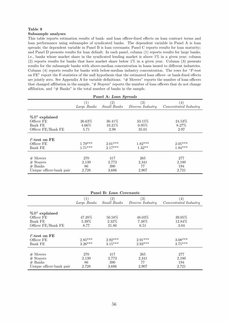
Table 9Subsample analysesThis table reports estimation results of bank- and loan officer-fixed effects on loan contract terms andloan performance using subsamples of syndicated banks. The dependent variable in Panel A is loanspreads; the dependent variable in Panel B is loan covenants; Panel C reports results for loan maturity;and Panel D presents results for loan default. In each panel, column (1) reports results for large banks,i.e., banks whose market share in the syndicated lending market is above 1% in a given year; column(2) reports results for banks that have market share below 1% in a given year. Column (3) presentsresults for the subsample banks with above-median concentration in loans issued to different industries.Column (4) reports results for banks with below-median industry concentration. The rows for “F -teston FE” report the F-statistics of the null hypothesis that the estimated loan officer- or bank-fixed effectsare jointly zero. See Appendix A for variable definitions. “# Movers” reports the number of loan officersthat changed affiliation in the sample, “# Stayers” reports the number of loan officers that do not changeaffiliation, and “# Banks” is the total number of banks in the sample.

Panel A: Loan Spreads

(1) (2) (3) (4)Large Banks Small Banks Diverse Industry Concentrated Industry

%R2 explainedOfficer FE 26.63% 30.41% 33.15% 24.53%Bank FE 4.66% 10.21% 0.95% 8.27%Officer FE/Bank FE 5.71 2.98 35.01 2.97

F -test on FEOfficer FE 1.79*** 2.01*** 1.82*** 2.05***Bank FE 1.71*** 2.17*** 1.32** 1.94***

# Movers 270 417 265 277# Stayers 2,139 2,773 2,341 2,100# Banks 86 390 77 194Unique officer-bank pair 2,728 3,686 2,907 2,721

Panel B: Loan Covenants

(1) (2) (3) (4)Large Banks Small Banks Diverse Industry Concentrated Industry

%R2 explainedOfficer FE 47.28% 50.58% 48.03% 39.05%Bank FE 5.39% 2.32% 7.38% 12.84%Officer FE/Bank FE 8.77 21.80 6.51 3.04

F -test on FEOfficer FE 2.85*** 2.92*** 2.91*** 3.08***Bank FE 3.26*** 3.15*** 2.93*** 3.75***

# Movers 270 417 265 277# Stayers 2,139 2,773 2,341 2,100# Banks 86 390 77 194Unique officer-bank pair 2,728 3,686 2,907 2,721

56

Panel C: Loan Maturity

(1) (2) (3) (4)Large Banks Small Banks Diverse Industry Concentrated Industry

%R2 explainedOfficer FE 31.06% 38.93% 34.50% 34.47%Bank FE 0.98% 5.19% 1.70% 4.70%Officer FE/Bank FE 31.86 7.51 20.35 7.33

F -test on FEOfficer FE 1.35*** 1.61*** 1.42*** 1.47***Bank FE 0.82 1.65*** 1.27* 1.53***

# Movers 270 417 265 277# Stayers 2,139 2,773 2,341 2,100# Banks 86 390 77 194Unique officer-bank pair 2,728 3,686 2,907 2,721

Panel D: Loan Performance (Default)

(1) (2) (3) (4)Large Banks Small Banks Diverse Industry Concentrated Industry

%R2 explainedOfficer FE 53.22% 52.02% 57.42% 56.62%Bank FE 1.47% 10.09% 1.61% 2.59%Officer FE/Bank FE 36.26 5.16 35.78 21.85

F -test on FEOfficer FE 3.07*** 3.67*** 3.22*** 3.63***Bank FE 2.04*** 4.05*** 2.26*** 4.09***

# Movers 270 417 265 277# Stayers 2,139 2,773 2,341 2,100# Banks 86 390 77 194Unique officer-bank pair 2,728 3,686 2,907 2,721

*** p <0.01, ** p <0.05, * p <0.1

57

Table 10Sub-period analysesThis table reports estimation results of bank- and loan officer-fixed effects on loan contract terms andloan performance from different sample periods. The first column describes the dependent variables ineach test. Column (1) reports the sub-periods. Column (2) reports the incremental R2 explained byofficer fixed effects relative to the baseline model. Column (3) presents the incremental R2 explained bybank fixed effects relative to the baseline model. Column (4) compares the relative explanatory powerof officer fixed effects relative to bank fixed effects (Officer FE/Bank FE). The baseline model controlsfor firm characteristics, loan terms (other than dependent variable), borrower industry fixed effects, andyear fixed effects.

(1) (2) (3) (4)

Dep. Var. Sub-period Officer incremental R2 Bank incremental R2 Relative

Loan Spreads 1994–2003 19.29% 1.99% 9.69

2004–2006 19.34% 0.62% 31.19

2007–2009 18.57% 2.03% 9.15

2010–2012 20.23% 2.06% 9.82

Loan Covenants 1994–2003 33.19% 2.82% 11.77

2004–2006 36.00% 3.36% 10.71

2007–2009 37.46% 3.42% 10.95

2010–2012 37.26% 3.65% 10.21

Loan Maturity 1994–2003 16.12% 0.83% 19.42

2004–2006 28.67% 2.73% 10.50

2007–2009 20.09% 1.84% 10.92

2010–2012 21.53% 1.96% 10.98

Default 1994–2003 35.62% 2.70% 13.19

2004–2006 34.90% 1.46% 23.90

2007–2009 43.35% 3.46% 12.53

2010–2012 19.00% 3.83% 4.96

*** p <0.01, ** p <0.05, * p <0.1

58

Table 11Loan officer heterogeneityThis table reports the correlation of loan officers’ lending styles. We first extract loan officer fixed effectsusing three-way fixed effects regressions using the method detailed in Abowd, Creecy, and Kramarz(2002). For detailed procedures, please see description in Table 4. After extracting loan officers’ fixedeffects in all aspects of lending activities, we examine the simple correlation between fixed effects.

Loan Spreads Loan Covenants Loan Maturity

Loan Covenants -0.0528***

Loan Maturity 0.0605*** -0.0323**

Default 0.1735*** 0.0407*** 0.0991***

*** p <0.01, ** p <0.05, * p <0.1

59

Tab

le12

Loan

offi

cer

hete

rogen

eit

yT

his

tab

lees

tim

ates

the

corr

elat

ion

oflo

anoffi

cer

per

form

an

cean

dth

eb

ack

gro

un

dch

ara

cter

isti

csof

thes

elo

an

offi

cer.

We

regre

ssth

ees

tim

ate

dfi

xed

effec

tsof

loan

office

ron

loan

contr

act

term

san

dlo

anp

erfo

rman

cem

etri

cson

loan

offi

cer

back

gro

und

chara

cter

isti

csex

tract

edfr

om

Lin

kedIn

info

rmati

on

.T

he

ind

epen

den

tva

riab

les

are

esti

mat

edoffi

cer

fixed

effec

ts,

coll

apse

dat

the

offi

cer

leve

l.F

irst

Ban

kS

ize

isth

em

ark

etsh

are

of

the

firs

tsy

nd

icate

dle

nd

erth

at

an

offi

cer

work

sat

afte

rgr

adu

atio

n.

Bu

sin

ess/

Eco

nD

egre

eis

anin

dic

ator

that

equ

als

on

eif

alo

an

offi

cer

ma

jors

inb

usi

nes

s(i

ncl

ud

ing

Fin

an

ce,

Acc

ou

nti

ng,

etc.

)or

econ

om

ics.

Top

Sch

ool

isan

ind

icat

orfo

rw

het

her

anoffi

cer

atte

nd

eda

top

ten

un

der

gra

du

ate

or

MB

Ap

rogra

m.

Fem

ale

isan

ind

icato

rfo

rw

het

her

the

loan

offi

cer

isfe

male

.C

ohort

Yea

ris

the

year

that

alo

anoffi

cer

ente

rsco

lleg

e.C

olu

mn

(6)

rep

ort

sth

eR

2fr

om

the

com

bin

edre

gre

ssio

ns.

Loan

offi

cer

fixed

effec

tsare

esti

mate

din

afi

rst

stag

ere

gres

sion

foll

owin

gth

em

eth

od

intr

od

uce

din

Ab

owd,

Kra

marz

,an

dM

arg

oli

s(1

999)

an

dA

bow

d,

Cre

ecy,

an

dK

ram

arz

(2002).

The

fixed

effec

tsare

then

nor

mal

ized

wit

hin

each

grou

pof

con

nec

ted

ban

ks

toh

ave

zero

mea

ns.

(1)

(2)

(3)

(4)

(5)

(6)

Dep

.V

ar.

Reg

ress

ion

Fir

stB

an

kS

ize

Bu

sin

ess/

Eco

nD

egre

eT

op

Sch

ool

Fem

ale

Coho

rtY

ear

R2

Loa

nS

pre

ads

Sep

arat

e86

.198

2***

0.9

792

13.4

813**

0.3

539

0.1

130

Tog

eth

er57

.298

913.4

738

18.2

356*

7.3

121

0.0

928

0.0

157

Loa

nC

ove

nan

tsS

epar

ate

0.84

36**

-0.0

361

0.0

958

0.1

082

-0.0

033

Tog

eth

er0.

7754

-0.0

240

-0.0

634

0.0

173

0.0

008

0.0

050

Loa

nM

atu

rity

Sep

arat

e-1

0.30

22**

0.3

033

1.6

043

0.6

298

0.0

875

Tog

eth

er-1

2.80

32**

-0.3

003

1.3

410

0.3

633

0.0

181

0.0

089

Def

au

ltS

epar

ate

0.20

94**

*-0

.0069

0.0

035

0.0

068

0.0

003

Tog

eth

er0.

1742

*0.0

115

-0.0

166

-0.0

135

0.0

008

0.0

075

60