CENTRE FOR APPLIED MACROECONOMICS AND COMMODITY PRICES (CAMP)

CAMP Working Paper Series No 12/2020

Do Central Banks Respond to Exchange Rate Movements? A Markov-Switching Structural Investigation of Commodity Exporters and Importers

Ragna Alstadheim, Hilde C. Bjørnland and Junior Maih

© Authors 2020 This paper can be downloaded without charge from the CAMP website.bi.no/camp

Do Central Banks Respond to Exchange Rate

Movements? A Markov-Switching Structural

Investigation of Commodity Exporters and Importers*

Ragna Alstadheim� Hilde C. Bjørnland� Junior Maih§

January 25, 2021

Abstract

We analyse whether central banks in small open commodity exporting and im-

porting countries respond to exchange rate movements, taking into consideration

that there may be structural changes in parameters and volatility throughout the

sample. Using a Markov Switching Rational Expectations framework, we estimate

the model for Australia, Canada, New Zealand, Norway, Sweden and the UK. We

find that the size of policy responses, and the volatility of structural shocks, have not

stayed constant during the sample. Furthermore, monetary policy has responded

strongly to the exchange rate in many commodity exporters, most notably in Nor-

way. This has had a stabilizing effect on the exchange rate. In particular, although

the terms of trade are highly volatile among commodity exporters, the exchange

rate has about the same volatility across all importers and exporters in the recent

period.

JEL-codes: C68, E52, Q4

Keywords: Monetary policy, exchange rates, commodity exporters, markov switching*We thank Zack Miller - the Guest Editor to the special issue in Energy Economics, two anonymous

referees, Yoosoon Chang, Sandra Eickmeier, Ibolya Schindele, participants at seminars in the ECB, IMF,

Norges Bank, the Central Bank of Budapest, The Central Bank of Armenia, and at the CEF conference

in Vancouver for constructive comments. This is a substantially revised version of a paper with title: ”Do

Central Banks Respond to Exchange Rate Movements? A Markov-Switching Structural Investigation”

This paper is part of the research activities at the Centre for Applied Macroeconomics and commodity

Prices (CAMP) at the BI Norwegian Business School. The views expressed in this paper are those of

the authors and do not necessarily reflect those of Norges Bank. The usual disclaimers apply.�Ragna Alstadheim, Norges Bank. Email: Ragna.Alstadheim@norges-bank.no�Corresponding author : Hilde C. Bjørnland, Centre for Applied Macroeconomics and commodity

prices (CAMP), BI Norwegian Business School. Email: hilde.c.bjornland@bi.no§Junior Maih, Norges Bank and Centre for Applied Macroeconomics and commodity prices (CAMP),

BI Norwegian Business School. Email: Junior.Maih@norges-bank.no

1

1 Introduction

During the last two decades an increasing number of small open economies have officially

abandoned their fixed exchange rate arrangements to allow their currencies to float within

an inflation targeting framework for monetary policy. More exchange rate flexibility is

associated with macroeconomic and financial stability (see Ghosh et al. (2015)), as well

as a requirement for monetary policy independence according to the classic monetary

policy trilemma (see Mundell (1963)). However, small open economies will be affected

differently by the global business cycles, depending on whether they are major exporters

or importers of commodities. As terms of trade is often very volatile in resource rich

countries, flexible exchange rates may not be enough to provide overall economic stability,

as well as guarantee monetary autonomy in a world of large capital flows, see e.g. Rey

(2016).1 Inflation targeting central banks may therefore want to respond to the exchange

rate to independently stabilize the economy.

Previous studies analyzing whether central banks respond to the exchange rate, how-

ever, have found conflicting evidence. In particular, Lubik and Schorfheide (2007) esti-

mate a small structural general equilibrium model for Australia, Canada, New Zealand

and the UK, and find that Canada and the UK include the exchange rate in their Taylor

rule. However, in another study, using more recent data, Dong (2013) finds that nei-

ther of the four countries show any clear evidence that they adjusted the interest rate in

response to the exchange rate.2

In this paper we take a different approach. Where previous studies have estimated

structural general equilibrium models with interest rate rules for monetary policy using

constant parameters, we will allow policy rule coefficients to change over time. In partic-

ular, there is ample reduced form evidence that the degree of exchange rate stabilization

has changed over time in many small open economies (see Ilzetzki et al. (2017a)), and

maybe more so for commodity exporters. Failure to also then allow parameters to change

when analysing the role of monetary policy in exchange rate stabilization could bias the

estimates, and explain the different results in the literature.

Against this background, we analyse whether central banks respond to exchange rate

changes in a framework allowing for regime changes to the monetary policy responses

and in the variance of shocks that hit small open economies. Our main aim is to explore

1Furthermore some also question the extent to which exchange rates are truly flexible, see Calvo and

Reinhart (2002).2In addition to having more recent data, the model setup also varies slightly, as Dong (2013) allows both

the terms of trade to be endogenous and incomplete pass-through beyond sticky-price-only set-up.

2

whether inflation targeting central banks in commodity exporting countries put the same

weight on stabilising the exchange rate throughout the period independently of the known

regime changes and the volatility of shocks, and also compared to commodity importing

countries. Furthermore, given that we observe a policy regime change, we analyse how

this may have impacted the responses of output and inflation to external shocks. A strong

or weak policy response to the exchange rate may imply larger or smaller volatility of

endogenous variables, depending on the cocktail of disturbances hitting the economy.

To answer these questions, we extend a small open economy dynamic stochastic gen-

eral equilibrium (DSGE) model to include a time-varying policy rule as well as time-

varying structural shocks. The constant parameter part of the model is similar in style

to the model in Galı and Monacelli (2005) and adapted also in Lubik and Schorfheide

(2007). Our aim of the paper is to shed light on the question about whether central banks

respond to exchange rate movements using a standard framework like that in Lubik and

Schorfheide (2007), but allowing for non-linearities.3

The time-variation that we allow for is modeled as independent Markov switching in

monetary policy responses on the one hand, and in the variances of structural shocks on

the other. With rational expectations, our model incorporates the fact that agents in the

economy realize that regime changes are possible at any time.4 To estimate the regime

switches, we use the Newton solution algorithm developed by Maih (2015), which extends

Farmer et al. (2011) by being more general and efficient. The model is estimated using

Bayesian techniques accommodating different regimes within one model. We estimate a

model where the parameters may switch simultaneously or independently, allowing for a

simultaneous inference on both the policy parameters and the stochastic volatilities.5

The analysis is applied (independently) to six small-open-economy countries: Aus-

tralia, Canada, New Zealand, Norway, Sweden and the UK, that are differently affected

by the global business cycle: Australia, Canada, Norway and New Zealand are commodity

exporters, of which Canada and Norway are major oil exporters. Sweden and the UK are

commodity importing countries. By analysing these countries we believe our results can

3Our model can be further improved by, say, allowing for endogenous terms of trade and incomplete

pass-through, as in Dong (2013). However, for the question we are trying to answer, we believe the

framework in Lubik and Schorfheide (2007) is sufficient.4This means that the so-called “peso problem” (see e.g. Evans (1996)) can be consistently dealt with in

our framework.5Our study is also unique in another important way; we don’t de-trend the data prior to estimation. We

believe non-filtered data are important to let the Markov-switching framework inform about medium-

term changes in the dynamics of the data, which detrending effectively eliminates. Our hypothesis is

that the variables can be stationary but from different distributions reflected by different regimes.

3

be generalized to a broader set of countries, and we are able to shed light on differences

in exchange rate policy between commodity exporters and importers. We use quarterly

data with the longest available sample possible: Starting in 1964 for Canada and the

UK; 1968 for Australia, 1974 for New Zealand and 1982 for Norway and Sweden. Over

the sample analysed, all countries have also formally abandoned exchange rate targeting

and adopted inflation targeting as a framework for monetary policy. Consistent with

the structural model, the exchange rate that countries potentially stabilize in our model

is measured as the nominal effective exchange rate (measured with time-varying trade

weights).

We have three main findings. First, there is strong evidence that neither policy

responses nor the volatility of structural shocks have remained constant throughout the

sample period in any of the six countries. For each country, we identify both a “high”

and “low” exchange rate response regime, as well as a “high” and “low” volatility regime.

Still, the timing of the policy parameter changes and the persistence of the high response

regime vary from country to country: Australia stands out and responds strongly to the

exchange rate only in certain brief periods early in the sample. In Sweden and the UK,

the central banks switch from a high to a low exchange rate response regime shortly after

severe periods of currency crisis and collapse of their fixed exchange rate regime - UK

after the collapse of the Bretton Woods system in 1972 and Sweden after the regime to

European Currency Union (ECU) broke down in 1992 and they adopt inflation targeting

(1993). The central banks in three of the commodity exporting countries Canada, New

Zealand and Norway, however, remain in a high response regime until the end of the

1990s, some time after adopting inflation targeting. For Norway, the central bank also

responds strongly to the exchange rate even after adopting inflation targeting. These are

new results in the literature, giving a more nuanced picture of the weights that central

banks give to stabilizing the nominal exchange rate. In particular, the results stand

in contrast to the perception one gets by observing official (”de jure”) monetary policy

frameworks.

Second, we show that policy rules with a high response to the exchange rate exacer-

bate the effects of external shocks on the domestic variables in advanced economies. In

particular, for resource rich Norway, that has responded strongly to the exchange rate in

most of the sample, the effect of the terms-of-trade shocks on output and inflation are

clearly exacerbated relative to the other countries. However, volatility of the terms of

trade is much higher in Norway than in the other countries, which is most likely due to

the size of the petroleum sector. Given this volatility, and a formal regime of inflation

4

targeting, it may seem surprising that the terms of trade shocks do not explain even

more of the variance in the nominal exchange rate in Norway than they do. The fact that

the central bank in Norway has stabilized the exchange rate somewhat more than in the

other countries may have contributed to this. Still, other objectives may be satisfied, and

exchange rate stabilization may be optimal given the different exposure to commodity

markets.6

Third, there is a striking similarity in the timing of the switch between the high

and low volatility regimes across countries, independently of the chosen policy rules.7

This suggests that common international volatility shocks may play a role, both for the

commodity exporters and the commodity importers in our sample.

Our paper contributes to a large literature on exchange rates and monetary policy,

see in particular Taylor (2001), Engel and West (2006), Galı and Monacelli (2005), Lubik

and Schorfheide (2007) and Clarida et al. (1998), that study from various perspectives

monetary policy response to nominal or real exchange rate changes.8 Relevant are also the

papers that analyse the interdependence between monetary policy responses and exchange

rates dynamics in an inflation targeting area, see for instance Scholl and Uhlig (2008),

Bjørnland (2009) and Bjørnland and Halvorsen (2014). To the best of our knowledge, our

paper is the first paper to address the specific question of regime shifts in the monetary

policy responses to the exchange rate.

Our work also contributes more generally to a broader literature that emphasizes the

importance of allowing for parameters and volatility of shocks to change when analysing

policy questions. So far, only a few papers in the literature address this issue in open

economies, see for instance Liu and Mumtaz (2011), Dybowski et al. (2018) and Jin

and Xiong (2020).9 However, changes in shock variances and/or studies of the great

moderation in closed economies such as the US have for some time been documented,

see e.g. Stock and Watson (2005), Sims and Zha (2006), Lubik and Schorfheide (2004),

6Similar arguments are also put forward ion Catao and Chang (2013) and De Paoli (2009).7Note, to economize on parameters and strengthen identification of different regimes, we let the switch in

variances for different shocks be synchronized (but can of course vary from country to country).8For an early article analysing exchange rate stabilization, see Obstfeld and Rogoff (1995), or, see Corsetti

et al. (2010) and Engel (2014) for more recent surveys on the large literature on monetary policy and

exchange rate determination.9Liu and Mumtaz (2011) is most related to us, as they analyse regime shifts in the UK using a Markov

switching open economy DSGE model, although the focus there is on changes in volatility and breaks

in structural parameters in general, and not on the open economy issues in particular. Dybowski et al.

(2018) estimate a time-varying parameter (TVP) Bayesian VAR model for Canada, while Jin and Xiong

(2020) analyse the link between the exchange rate and oil prices in Russia, using a Markov switching

framework.

5

Smets and Wouters (2007), and Bjørnland et al. (2018). Through our Markov Switching

framework we are able to compare the estimated effects of shocks, across different types of

monetary policy regimes, and across countries where exports are important to a varying

degree. Thus, the fact that we are applying the same analysis across small open economies

and yet get different results for the various countries, is a strong indication that we are

picking up relevant information about changing regimes in open economies.

Finally, our paper is also related to the literature on exchange rate regime classifica-

tion. The development of exchange rate regimes over time is well documented in Ilzetzki

et al. (2017a), Ilzetzki et al. (2017b) and Klein and Shambaugh (2012). In particular,

the “bipolar view” of exchange rate regimes, where countries either tend to let their ex-

change rate float relatively freely or firmly peg their exchange rates, is not an accurate

description of reality, see e.g. Brooks et al. (2004). This paper provides results consistent

with multiple changes in the adopted regimes.

The remainder of the paper is structured as follows. We start by discussing some

stylized facts and acknowledging the periods of known policy changes in Section 2. Section

3 describes the New Keynesian model for small open economies (SOE) which is extended

with regime switching, while the solution algorithms are described in Section 4. Data,

priors and details on estimation procedure are presented in Section 5, and the results are

reported in Section 6. Section 7 discusses robustness, and Section 8 concludes.

2 Stylized facts and known policy changes in ad-

vanced small open economies

While the six countries we analyse are all small and open inflation targeting countries,

the dates for when they adopted an inflation targeting framework vary, see Ilzetzki et al.

(2017b): Commodity exporter New Zealand was the pioneer, creating inflation targeting

as a concept and establishing it by law in 1989. Their background was a history of

exchange rate targeting but an unstable inflation rate. The regime in New Zealand

became more flexible over time, after a quite rigid start, see McDermott and Williams

(2018). Oil exporter Canada was the next country to adopt inflation targeting. In

Canada, the exchange rate was pegged to the US dollar until 1970, thereafter it stayed

within a narrow band, before it floated in 1973. Eventually Canada adopted an inflation

target in 1991, but has changed the explicit target and range several times since then, see

Bordo et al. (1999). However, since the end of 1995, the target for the annual rate of total

6

consumer price inflation has been the 2 percent midpoint of a 1 to 3 per cent range.10 The

next two nations to adopt inflation targeting were UK and Sweden. They switched to

inflation targeting in October 1992 and January 1993 respectively, after currency crises

and the collapse of their fixed exchange rate regimes to the ECU in the fall of 1992. In so

doing, UK was the first country in Europe to adopt inflation targeting. The countries have

adhered to a policy of not intervening systematically in the foreign exchange market since

then. Note that although Sweden formally announced inflation targeting in 1993, it was

not applied before 1995. Australia was in 1993 the next adopter of inflation targeting.

In commodity exporter Australia, the transition to the new regime happened without a

reform of the legal framework, as in New Zealand, and also without a dramatic exit from

a fixed exchange rate regime, as in Sweden and the UK. Instead, the transition has been

described as “evolutionary rather than revolutionary”, see Debelle (2018). Oil exporter

Norway has had a history of various fixed exchange rate arrangements. Interventions

to fix the Norwegian krone were abandoned in December 1992, and the foreign exchange

regime thereafter became more flexible, see Alstadheim (2016). Monetary policy was still

oriented towards maintaining a stable exchange rate in relation to European currencies

(but now without defining a central exchange rate to be defended by interventions). Yet

with volatile terms of trade, this became challenging. From 1999, monetary policy was

more explicitly geared towards stable consumer price inflation though, and eventually, in

early 2001, a formal inflation targeting framework was adopted in Norway as well.

The above discussion of formal regime changes illustrates several reasons why esti-

mating exchange rate responses with a split sample is not satisfactory: First, the an-

nouncement of official (“de jure”) inflation targeting (and flexible exchange rates) may

not come at the same time as the actual adoption of (“de facto”) inflation targeting

and more exchange rate flexibility. A country may want to gradually adapt to the new

target, see Reinhart and Rogoff (2004). Secondly, inflation targeting is often practised

flexibly, taking into account other goals such as the stability of output, and also - directly

or indirectly - exchange rate fluctuations. It is therefore not obvious how to split the

sample based on formal policy change. Our approach is therefore to examine the relevant

parameters in a structural model, in order to uncover evidence of (”de facto”) changed

behavior by policymakers.

Finally, stylized facts suggest there have been large changes in the volatility of macroe-

conomic variables over the sample we are analysing, changes which are important to in-

10Note, however, that until September 1998, the Bank of Canada intervened in the foreign exchange market

in a systematic and automatic fashion to avoid significant upward or downward pressures on the Canadian

dollar. Since September 1998, the policy has been to intervene only in exceptional circumstances.

7

Table 1: Stylized facts

AU CA NZ NO SW UK

Exchange rate 3.78/4.01 1.60/2.95 3.55/3.43 1.58/2.34 3.30/2.50 3.10/2.41

Terms of trade 3.46/3.05 1.27/2.08 3.85/2.69 4.23/5.05 1.88/1.23 1.94/0.88

GDP 1.24/0.56 1.13/0.58 1.32/0.96 1.28/1.27 1.18/1.12 1.13/0.58

Inflation 1.18/0.54 0.80/0.55 1.55/0.50 0.68/0.51 0.82/0.41 1.56/0.65

Interest rate 4.06/1.44 3.28/1.86 0.45/0.22 1.83/2.03 1.78/2.35 2.97/2.31

Note: Each cell reports the standard deviations in the period prior to 1993 to the left and in the period

post 1993 to the right. Start dates reflects data availability, see section 5.1.

corporate when analysing our question of interest. Table 1 illustrates this, by reporting

standard deviations of some key macro variables before and after the exchange rate tur-

bulence in 1992/1993.11 There are three key findings: First, we find that volatility has

declined over time for GDP and inflation in all six countries, although for New Zealand

the decline in GDP volatility is negligible. On the other hand, the decline in volatility of

inflation is substantial for all countries, and in particular for New Zealand and the UK.

Hence, good policies (i.e. adopting an inflation targeting framework instead of target-

ing the exchange rate) and maybe also good luck, have made the small open economies

overall more stable.

Second, volatility of terms of trade have fallen in the post 1993 period for all countries

but Canada and Norway. This is not very surprising, given that these two countries are

important oil and gas exporters. High volatility in oil prices is reflected in the terms of

trade. Still, volatility remains quite high also after 1993 in the other two resource rich

countries Australia and New Zealand. Norway stands out, however, with terms of trade

being almost 5 times as volatile compared to UK, which has the lowest volatility in terms

of trade.

Third, despite this, the exchange rate has about the same volatility across the coun-

tries in the recent inflation targeting period, but with Australia and New Zealand at the

higher end, and the three European countries, Norway, Sweden and the UK, at the lower

end. This could suggests that monetary policy has had a role to play in the stabilizing of

the exchange rate (and subsequently inflation), eventhough these countries have adopted

inflation targeting and are both commodity exporters and importers. Hence, by respond-

ing (flexibly) to the exchange rate, they may also have managed to shelter the economy

from terms of trade fluctuations, and better stabilize the economy. We now formally

11By 1993, all countries had formally given up targeting the exchange rate.

8

address these issues using a structural model.

3 A regime-switching small open economy model

Our model is a simplified version of Galı and Monacelli (2005), adapted from Lubik and

Schorfheide (2007),12 However, in contrast to these papers, our model accommodates

independent Markov switching in the structural shocks that hit the economy and in

the monetary policy responses. That is, we will allow some parameters to be drawn

from different distribution, so they can switch through time. Additional details on the

estimation of the Markov switching framework will be given in Section 4. Here we focus

on explaining how we have extended the model in Galı and Monacelli (2005), with regime

switches.

In brief, the model consists of a forward-looking (open economy) IS equation, a Phillips

curve, an exchange rate equation and a monetary policy (interest rate) rule. Below we

present the model framework. Following Lubik and Schorfheide (2007), we rewrite the

(consumption) Euler equation as an open economy IS-curve:

yt = Etyt+1 − (τ + λ)(it − Etπt+1)− ρzzt − α(τ + λ)Et∆qt+1 +λ

τEt∆y

∗t+1, (1)

where 0 < α < 1 is the import share (that measures the degree of openness), τ is the

intertemporal substitution elasticity and we define λ = α(2 − α)(1 − τ). Note that the

equation reduces to its closed economy variant when α = 0. The endogenous variables

are output yt, the CPI inflation rate πt and the nominal interest rate it. qt is the terms

of trade, y∗t is world output, while zt is the growth rate of an underlying non-stationary

world technology process At. It is assumed that y∗t and zt are exogenous variables that

evolve as AR processes with autoregressive coefficients ρy∗ and ρz respectively.

Optimal price setting of domestic firms, together with an assumption of perfect risk-

sharing across countries that links domestic potential output to foreign output, leads to

the open economy Phillips curve

πt = βEtπt+1 + αβEt∆qt+1 − α∆qt +κ

(τ + λ)(yt − yt), (2)

where yt ≡ −α(2−α)(1− τ)/τy∗t is domestic potential output in the absence of nominal

rigidities. Again this reduces to the closed economy variant with α = 0. In a standard

New-Keynesian model, κ is the slope coefficient. It is related to the price stickiness,

the degree of competition and the representative firm’s cost function parameters. Like

12See also Del Negro and Schorfheide (2009) for a similar exposition.

9

Lubik and Schorfheide (2007), we treat κ itself as structural, but we do not model the

underlying structure of the production side of the economy. Finally, when estimating the

model, we add a demand shock εy to the IS equation and a cost push shock επ to the

Phillips curve.

We introduce the nominal exchange rate (et) via the definition of the real exchange

rate, rert = ∆et − πt + π∗t , where π∗t is world inflation. The real exchange rate is

proportional to the terms of trade in this model. With rert = (1−α)∆qt, the definition of

the real exchange rate then gives, up to a first order approximation, the following process

for the nominal exchange rate in our model:

∆et = πt − (1− α)∆qt − π∗t , (3)

The nominal exchange rate, domestic inflation, the terms of trade and foreign inflation

are all observable variables. Of these, the exchange rate and the domestic inflation rate

are endogenous, while the other variables will be exogenous and follow AR-processes.13

Finally, the assumption of proportionality between the real exchange rate and the terms

of trade does not hold exactly empirically, and we thus allow for measurement errors in

this equation.14

Monetary policy is described by an interest rate rule where we assume that the central

bank can adjust its instrument in response to inflation, output and the nominal exchange

rate depreciation:

it = ρi(SPolt )it−1 + (1− ρi(SPol

t ))(γπ(SPolt )πt + γy(SPol

t )yt + γe(SPolt )∆et) + εr,t. (4)

By adding the nominal exchange rate to the more standard Taylor rule, the rule en-

compasses periods of exchange rate targeting and inflation targeting, which are the two

regimes that we are interested in.15 We assume that the policy coefficients γπ, γy and γe

13Note that while we specify the terms-of-trade to be exogenous, it can be decided endogenously from the

model, as underscored by e.g. Del Negro and Schorfheide (2009). The same authors stick to exogenous

terms-of-trade in their estimation, as they find the impulse responses using an endogenous terms of trade

specification to be very similar. Still, as many of the variables in our estimation are observable, including

the terms-of-trade, a tighter specification of the terms-of-trade equation would be challenging, see also

Canova et al. (2014).14Implicitly, equation (3) also imposes a tight UIP-condition, since changes in the real exchange rate map

into a difference between real interest rates, and by implication between nominal interest rates and

inflation rates at home and abroad. The measurement errors can thus alternatively be interpreted as

allowing for UIP-deviations.15Note that the rule indirectly also encompasses real exchange rate stabilization, in that a stabilization

of the inflation rate as well as the nominal exchange rate change also stabilizes the real exchange rate,

see e.g. Galı and Monacelli (2005), Lubik and Schorfheide (2007), Clarida et al. (1998), Taylor (2001),

Engel and West (2006) and Caputo and Herrera (2017) for previous studies.

10

≥ 0. We also allow for a smoothing term in the rule, with 0< ρi < 1. εi,t is the exoge-

nous monetary policy shock, which can be interpreted as the unsystematic component of

monetary policy (deviation from the rule). Importantly, we allow all parameters that the

monetary authorities have control over to switch throughout the sample in the following

way:

SPolt ∈ {High, Low}.

Hence, the parameters ρi, γπ, γy and γe are allowed to follow an independent two-state

Markov process, where we denote the low response regime as (SPolt = Low) and the high

response regime as (SPolt = High).16 To compare systematically across countries, we

normalize the high response regime to be the regime where the central bank responds

strongly to the exchange rate, taking also into account the interest rate smoothing, i.e.,

(1− ρi(SPolt = High))γe(SPol

t = High) > (1− ρi(SPolt = Low))γe(SPol

t = Low).

Turning to the terms of trade, instead of solving endogenously for the terms of trade, we

follow Lubik and Schorfheide (2007) and add a law of motion for their growth rate to the

system:

∆qt = ρq∆qt−1 + εq,t (5)

Finally, we assume that the volatility of the shocks in the model can follow an in-

dependent two-state Markov process, of low and high volatility. As motivated above,

different policy responses may also reflect changes in volatility. In particular, some infla-

tion targeting central banks may, in certain periods, have a specific interest in explicitly

reacting to and smoothing exchange rate movements as a predictor of domestic volatil-

ity. Hence, assuming a time-invariant parameter reaction function as well as constant

volatility during the sample period may bias the results.

Hence, we allow the volatility of shocks to the variables to change over time;

SVolt ∈ {High, Low},

where we denote the low volatility regime as (SVolt = Low) and the high volatility regime

as (SVolt = High). Note that data will determine if the other variables are observing

16To economize on parameters, and given our very flexible model specification, a natural and reasonable

identifying assumption for regime change is that all policy rule parameters in a given country change at

the same time. We want to identify significant changes in policy, and we achieve this by requiring the

parameters to switch in a synchronized fashion. We label the regimes that we identify according to the

strength of the exchange rate response. However, it is not necessarily the case that all coefficients change

by much even if a regime change is identified.

11

the same pattern of high and low volatility. To compare systematically across countries,

we normalize the high volatility regime to be the regime where volatility (in output) is

highest, i.e.

σy(SVolt = High) > σy(SVol

t = Low).

Below we describe the Markov switching framework in more detail.

4 Markov Switching Rational Expectation framework

For each country, we will estimate a Markov switching model that allows for switching in

volatility and parameters in the monetary policy rule. For completeness we also estimate

three variants of the model with either time invariant regimes, switching in volatilities

only or switching in parameters in the policy rule only. With four countries this implies

that we will estimate a total of 16 models.17 Below we will describe details.

The model outlined above can be cast in a general Markov Switching DSGE (MS-

DSGE) framework

Et

h∑rt+1=1

prt,rt+1drt (xt+1 (rt+1) , xt (rt) , xt−1, εt) = 0, (6)

where Et is the expectation operator, drt : Rnv −→ Rnd is a nd × 1 vector of possibly

nonlinear functions of their arguments, rt = 1, 2, .., h is the regime a time t, xt is a nx× 1

vector of all the endogenous variables, εt is a nε× 1 vector of shocks with εt ∼ N (0, Inε),

prt,rt+1 is the transition probability for going from regime rt in the current period to

regime rt+1 = 1, 2, .., h in the next period and is such that∑h

rt+1=1 prt,rt+1 = 1.

We are interested in solutions of the form

xt (rt) = T rt (wt) , (7)

where wt is an nw × 1 vector of state variables.

In general, there is no analytical solution to (6) even in cases where drt is linear.

Maih (2015) develops a perturbation solution technique that allows us to approximate

the decision rules in (7) . The vector of state variables is then

wt ≡[x′t−1 σ ε′t

]′,

where σ is a perturbation parameter.

17In the robustness section we re-estimate all models using a shorter sample period, implying that we

estimate another 16 models, that is, 32 models in total.

12

The solution of our model takes the form

T rt (w) ' T rt (wrt) + T rtw (wt − wrt) , (8)

where wrt is the steady state values of the state variables in regime rt.

This solution is computed using the Newton algorithm of Maih (2015), which extends

that of Farmer et al. (2011), henceforward FWZ. In particular, the algorithm is more

general and efficient, as it solves a smaller system than FWZ by avoiding the computation

of expectational errors. Furthermore, the algorithms avoids building and storing large

Kronecker products and without inverting large matrices. This makes the algorithm

suitable for large systems.18

This type of solution in (8) makes it clear that the framework allows the model

economy to be in different regimes at different points in time, with each regime being

governed by certain rules specific to the regime. In that case the traditional stability

concept for constant-parameter linear rational expectations models, the Blanchard-Kahn

conditions, cannot be used. Instead, following the lead of Svensson and Williams (2007)

and Farmer et al. (2011) among others, this paper uses the concept of mean square

stability (MSS) borrowed from the engineering literature, to characterize stable solutions.

5 Data and Bayesian estimation

We estimate the parameters in the model with Bayesian methods using the RISE toolbox

in Matlab. The equations of the system are coded up using the RISE language in a text

file. The software takes the file containing the equations and automatically computes

the perturbation solution as well as the state-space form that is used for the likelihood

computation. For a regime-switching model like ours, the computation of the likelihood

has to be done via a filtering algorithm due to the presence of unobservable variables.

An exact filtering procedure that will track all possible histories of regimes is infeasible.

One solution described by Kim and Nelson (1999) consists of collapsing (averaging) the

forecasts for various regimes in order to avoid an explosion of the number of paths.

An alternative approach, the one we follow, is to collapse the updates in the filtering

procedure. This approach yields numerically similar results as the Kim and Nelson filter

but has the advantage of being computationally more efficient, see Maih (2015).

18The algorithm has been used in the solving of a system of upwards of 300 equations.

13

5.1 Data

The estimation is based on quarterly time-series observations for the period 1964Q1-

2015Q1 for Canada and the UK, 1968Q1-2015Q1 for Australia, 1974Q2-2015Q1 for New

Zealand while for Norway and Sweden, the sample runs from 1982Q1 to 2015Q1. The

start dates reflect data availability for the interest rate series and exchange rate series. For

each country, there are seven observable variables: Real GDP, inflation, the short term

interest rate, the nominal (trade weighted) effective exchange rate, the terms of trade and

foreign output and inflation. Note that in contrast to Lubik and Schorfheide (2007) who

treat foreign output and inflation as unobservable (latent) variables, we include foreign

output and inflation explicitly as observables in the model in order to better identify

the effects of foreign shocks. This ties the dynamics of the small open economies model

more explicitly to the global shocks. We approximate foreign output and foreign inflation

for each country based on the time-varying weights that were also used to calculate the

effective exchange rate. As far as possible, we collect data from the national sources. All

data except the nominal interest rate and the exchange rate are seasonally adjusted.

Regarding the transformation, output growth rates are computed as log differences of

GDP and multiplied by 100 to convert them into quarter to quarter percentages. Inflation

rates are defined as log differences of the consumer price indices and multiplied by 400

to obtain annualised percentage rates. We use the log differences (multiplied by 100) of

the trade-weighted nominal effective exchange rate to obtain depreciation rates (seen as

an increase). Percentage changes in the terms of trade are computed as log differences

and multiplied by 100 while the nominal interest rate is measured in levels. More details

about sources and transformations are given in Appendix A.

5.2 Choice of priors and estimation

Besides the model equations and the data, another input has to be provided for us to

do Bayesian estimation: the prior information on the parameters. Rather than setting

means and standard deviations for our parameters as it is customarily done, we set our

priors using quantiles of the distributions. Specifically, we use the 90 percent probabil-

ity intervals of the distributions to uncover the underlying hyperparameters. With the

exception of the parameter α, we allow for loose priors to entertain the idea that there

have been multiple regime changes in the sample. α, which is the import share, is tightly

centered around 0.2, as in Lubik and Schorfheide (2007).

The full list of our prior assumptions along with the posterior mode are reported in

Table 3. To compute the posterior kernel, the software (RISE) combines the (approxi-

14

mated) likelihood function with the prior information.19 The sampling of the posterior

distribution is not an easy task and there is no guarantee, in a complicated model like

ours in which the posterior density function is multimodal, that the posterior distribution

will be adequately sampled or that the optimization routines used will find the global

peak of the posterior distribution of the parameters. We exploit the stochastic search

optimization routines of the RISE toolbox to estimate the mode. Our stochastic search

approach is based on the Artificial Bee Colony (ABC) optimization (see Karaboga and

Akay (2011)).20 The algorithm alternates between phases of exploration (global search)

and phases of exploitation (local search) and avoids stalling by randomly restarting the

locations in which exploitation does not lead to any improvement of the likelihood.21

With a mode or starting point in hand, our strategy to simulate the posterior dis-

tribution is to run 5 parallel chains of the Adaptive Parallel Tempering (Miasojedow

et al. (2012)), a generic Markov chain Monte Carlo sampling method which allows good

mixing with multimodal target distributions, where conventional Metropolis-Hastings al-

gorithms often fail. The adaptive algorithm tunes both the temperature schedule, which

efficiently copes with multimodality22, and the parameters of the random-walk Metropo-

lis kernel automatically. In particular, the scale parameter in particular is adapted so as

to maintain an acceptance ratio of about 0.234.

The whole process is rather computationally intensive. For a given parameter draw,

the first-order perturbation solution of the model is computed following the Newton

algorithms described in Maih (2015), setting the convergence criterion to the square root

of machine epsilon. If a solution is found, it is checked for MSS. If the MSS test is passed,

the likelihood of the data is computed using the solution found and then combined with

the prior distribution of the parameters. This process, which has to be repeated millions

of times, takes several weeks to complete. We monitor convergence using various tools

such as trace plots as well as the Potential Scale Reduction Factor statistic as outlined

in Gelman et al. (2004).

19To specify the priors we use quantiles. It is customary in the literature to set priors in terms of means and

standard deviations. This does not necessarily work the other way around. That is for given quantiles,

we do not necessarily have corresponding means and standard deviations.20This optimization technique is inspired from the intelligent behavior of honey bees. Artificial bees fly

around a potentially multidimensional search space and adjust their position in the landscape according

to the amount of food (likelihood) that is found in various locations.21In our experience, the algorithm is easily capable of improving the solutions found by Newton-based

optimization techniques such as e.g. Matlab’s fmincon or Christopher Sims’ csminwell.22We apply twelve levels of tempering that progressively transform an almost uniform distribution into the

posterior kernel.

15

6 Results

We start out by estimating the parameters in a time invariant model before turning to

our preferred regime switching model; a model where both parameters and volatility are

allowed to switch over time. As stated above, the sample runs from 1964Q1 to 2015Q1

for Canada and the UK, from 1968Q1 to 2015Q1 for Australia, from 1974Q2 to 2015Q1

for New Zealand, while for Norway and Sweden, the sample runs from 1982Q1 to 2015Q1.

Eventually we will test robustness to starting the analysis in 1982 for all countries.

6.1 Time invariant Rational Expectation benchmark

The estimation results for the posterior mode, along with the prior distribution using a

time invariant (constant) model is reported in Table 2. For ease of exposition, we report

here only the parameters in the policy rule, other parameters can be obtained at request.

Table 2: Priors and Posterior mode of policy rule

Params P.distr P.prob low high AU CA NO NZ SW UK

ρi beta 0.90 0.40 0.75 0.79 0.84 0.93 0.88 0.78 0.80

γπ gamma 0.90 0.90 3.00 0.13 0.17 0.50 0.54 0.09 0.19

γy gamma 0.90 0.10 3.00 2.49 3.35 1.14 0.36 1.31 2.88

γe gamma 0.90 0.05 3.00 0.01 0.04 2.18 0.50 0.00 0.01

The table suggests policy rules that have a high weight on output and a small weight

on inflation. With regard to the exchange rate, the central bank in Norway respond

strongly to the exchange rate, whereas in the other countries, the response is small or

negligible. Hence, from these results we would conclude that only the central bank in

Norway responds strongly to the exchange rate.

Are these parameters reasonable? First, we note that when including the exchange

rate in the interest rate reaction function, the response to inflation becomes lower in a

standard Taylor rule. This is as expected, as the response goes via the exchange rate

also. More importantly, given our long sample, and the many known policy changes,

estimating constant parameter models over the sample may seem very restrictive. In

fact, we would argue that if the data are generated by different distributions reflected

by different regimes, forcing a time invariant distribution to the data should potentially

yield different results depending on the sample analysed. Thus, we can anticipate that

there will be a more nuanced picture when we allow the parameters to switch between

different regimes. We turn to this now.

16

6.2 A model with switching policy rule and volatility

The used procedure allows the likelihood to be evaluated at each point in time under

the different regimes. This information, through a Bayesian filtering scheme, is used to

update the probabilities of being in different states. So even if there was only one outlying

observation (perhaps a switch to inflation targeting), the estimation procedure would still

pick it up. But we do not just have one outlying observation, we have at least a decade of

inflation targeting after periods of fixed exchange rates. This allows us to better evaluate

both the switch in regimes and the duration of the regimes.

Economic reasoning suggests that it may be useful to allow both the parameters and

the volatility to potentially switch over time. Still, we could use a statistical criteria

to evaluate if such a regime switching model gives an accurate description of the data.

Table 4 in Appendix B provides such an evaluation by comparing the log Marginal Data

Density (MDD) Laplace approximation for the constant model with three alternative

regime switching models; a model with switches in the parameters only, a model with

switches in volatility only and our preferred model with both switches in volatility and

parameters.23 The results confirm that models that allow for switches in either policy

parameters and/or volatility are preferred to a constant parameter model in all countries.

Still, the most preferred model is the model that allows for switches in both parameters

and volatility, such as the one we estimate here. In the robustness section, however, we

will discuss robustness to some other alternative model specifications.

Table 3 displays the posterior mode of the estimated parameters in our preferred

model with switches in both policy responses and volatility of the structural shocks. We

find that the size of the policy responses, and the volatility of structural shocks, have not

remained constant during the different sample periods. First, for all countries, interest

rate smoothing is more pronounced in the low exchange rate response regime, as central

banks seem to minimize interest rate changes. The exchange rate regime is normalised

taking also into account the interest rate smoothing parameter. Independent of that,

we find that in the high response regime, Norway has by far the strongest response to

the exchange rate, followed by Sweden and the UK. In fact, for Norway the response is

substantial also in the low response regime, followed by New Zealand.24 We note here that

23Because the likelihood we work with is only approximate, we use the laplace approximation to the

posterior distribution, see Christiano et al. (2011) for details on computation.24Note that the exchange rate behavior may be affected by fiscal policy in commodity exporting countries,

via public commodity export revenues being invested abroad (in effect amounting to scheduled or non-

discretionary foreign exchange interventions, with reserves being held by the government rather than the

central bank).

17

Lubik and Schorfheide (2007) did not find that New Zealand responds to the exchange

rate. We believe that the added observables in our setup, combined with realistic flexibilty

that regime switching provides, allows for better identification of parameters.

For the other countries, the response is close to zero in the low response regime.

Hence, the picture is nuanced relative to the constant parameter model. Interestingly, it

is the three European countries that respond the most, that also have the most stable

exchange rate in the inflation targeting period, c.f. the stylized facts in Table 1.

With regard to the other policy parameters, for most countries the interest rate re-

sponds more strongly to inflation and output in the low response regime. Exceptions

are Australia and Norway, where the interest rate responds more strongly to output in

the high response regime. However, given that the interest rate smoothing is also more

pronounced in the low response regime, the low response regime can be characterized by

an interest rate rule that emphasises interest rate smoothing and strong inflation and

output response, while the high response regime is characterized by strong exchange rate

response, and for Norway, also substantial output response. Interestingly, with regard

to the size of the estimated parameters, the responses to output in the low response

regime have now declined substantially relative to the constant parameter model, while

the responses to inflation and the exchange have increased.

Regarding the Markov state processes for volatility, most shocks display the highest

volatility in regime (SVolt = High). For all countries, the probability of moving from a

high to a low volatility regime is greater than moving from a low to a high volatility

regime. Note that Norway stands out from the other countries in that volatility of terms

of trade is 2-3 times higher than in the other countries (in both the low and high volatility

regime), see Table 3. This is most likely due to the relative size of the petroleum sector in

that country. Still, despite this high volatility in the terms of trade, output and inflation

do not display much higher volatility in Norway than in the other countries. This may

suggest that by responding strongly to the implied exchange rate volatility, they are also

able to partly shelter the domestic economy from the volatile terms of trade shocks, as

emphasized first when we discussed stylized facts. We turn to this in more detail below.

Finally, with respect to the other structural parameters (that are not switching),

most parameters seem to be within reasonable values. We note that the parameter α

that measures the degree of openness, is estimated to be the largest in Norway, followed

by Sweden, Canada and the UK. Hence, by that measure Norway is the most open coun-

try. Interestingly, these four countries are also those that observe the most pronounced

response to the exchange rate in the high response regime.

18

Table 3: Priors and posterior mode

Params P.distr P.prob low high AU CA NO NZ SW UK

τ beta 0.90 0.17 0.83 0.19 0.17 0.51 0.15 0.37 0.17

k gamma 0.90 0.12 0.87 0.05 1.23 3.94 2.37 2.88 1.68

α beta 0.90 0.12 0.28 0.16 0.05 0.41 0.12 0.17 0.07

ρq beta 0.90 0.10 0.80 0.27 0.30 0.57 0.36 0.23 0.07

ρy∗ beta 0.90 0.40 0.80 0.93 0.97 0.83 0.96 0.97 0.96

ρπ∗ beta 0.90 0.10 0.80 0.97 0.81 0.97 0.81 0.85 0.93

ρz beta 0.90 0.40 0.80 0.38 0.33 0.85 0.59 0.56 0.29

coef tp L H beta 0.90 0.00 0.10 0.03 0.00 0.00 0.00 0.01 0.00

coef tp H L beta 0.90 0.00 0.10 0.12 0.01 0.01 0.01 0.06 0.04

ρi(SPolt = Low) beta 0.90 0.40 0.75 0.94 0.91 0.96 0.93 0.90 0.91

ρi(SPolt = High) beta 0.90 0.40 0.75 0.47 0.82 0.92 0.84 0.73 0.72

γπ(SPolt = Low) gamma 0.90 0.90 3.00 0.17 0.77 0.57 0.65 0.96 0.82

γπ(SPolt = High) gamma 0.90 0.90 3.00 0.16 0.58 0.57 0.49 0.95 0.82

γy(SPolt = Low) gamma 0.90 0.10 3.00 2.58 0.22 0.06 0.22 0.23 0.28

γy(SPolt = High) gamma 0.90 0.10 3.00 2.60 0.04 0.21 0.09 0.04 0.16

γe(SPolt = Low) gamma 0.90 0.05 3.00 0.00 0.07 2.03 0.24 0.00 0.07

γe(SPolt = High) gamma 0.90 0.05 3.00 0.30 0.27 2.49 0.35 0.91 0.71

vol tp L H beta 0.90 0.00 0.10 0.01 0.02 0.04 0.01 0.03 0.06

vol tp H L beta 0.90 0.00 0.10 0.02 0.05 0.13 0.06 0.12 0.09

σi(SV olt = Low) inv gamma 0.90 0.01 1.00 0.00 0.00 0.00 0.00 0.00 0.00

σi(SV olt = High) inv gamma 0.90 0.01 1.00 0.00 0.00 0.01 0.01 0.01 0.00

σq(SV olt = Low) inv gamma 0.90 0.01 1.00 0.02 0.01 0.05 0.02 0.01 0.01

σq(SV olt = High) inv gamma 0.90 0.01 1.00 0.04 0.03 0.07 0.04 0.03 0.02

σz(SV olt = Low) inv gamma 0.90 0.01 1.00 0.00 0.01 0.00 0.00 0.00 0.00

σz(SV olt = High) inv gamma 0.90 0.01 1.00 0.01 0.01 0.00 0.01 0.01 0.01

σy∗(SV olt = Low) inv gamma 0.90 0.01 1.00 0.00 0.00 0.00 0.00 0.00 0.00

σy∗(SV olt = High) inv gamma 0.90 0.01 1.00 0.00 0.01 0.01 0.01 0.01 0.00

σπ∗(SV olt = Low) inv gamma 0.90 0.01 1.00 0.00 0.01 0.00 0.01 0.01 0.00

σπ∗(SV olt = High) inv gamma 0.90 0.01 1.00 0.02 0.03 0.00 0.02 0.02 0.01

σy(SV olt = Low) inv gamma 0.90 0.01 1.00 0.00 0.00 0.00 0.00 0.00 0.00

σy(SV olt = High) inv gamma 0.90 0.01 1.00 0.01 0.00 0.01 0.00 0.01 0.01

σπ(SV olt = Low) inv gamma 0.90 0.01 1.00 0.03 0.01 0.01 0.01 0.01 0.01

Continued on next page

19

– Continued from previous page

Params P.distr P.prob low high AU CA NO NZ SW UK

σπ(SV olt = High) inv gamma 0.90 0.01 1.00 0.05 0.01 0.07 0.01 0.01 0.05

stderr DCPI inv gamma 0.90 0.01 0.10 0.01 0.01 0.01 0.01 0.01 0.01

stderr DFCPI inv gamma 0.90 0.01 0.10 0.00 0.00 0.00 0.00 0.00 0.00

stderr DGDP inv gamma 0.90 0.01 0.10 0.00 0.01 0.01 0.01 0.01 0.00

stderr DFGDP inv gamma 0.90 0.01 0.10 0.01 0.01 0.01 0.01 0.01 0.01

Figure 1 displays the smoothed probabilities of being in the high policy response,

(SPolt = High) while Figure 2 displays the probability of being in a high volatility regime

(SVolt = High). The figures emphasise that all the central banks but Australia switched

from a high to a low response regime at some point in the sample. Australia stands

out in the sense that they have responded on-off to the exchange rate during certain

brief periods, ending around 1996. UK also stands out, in the sense that they only

responded strongly early in the sample; around 1971/1972. This period corresponds well

with the end of the Bretton Woods system, an exchange rate arrangement where the US

dollar was tied to gold.25 After the US dollar’s convertibility into gold was suspended in

August 1971, several countries that had pegged their currencies to the US dollar changed

their arrangements. UK abandoned the peg in June 1972 and adopted instead a moving

band around the Deutchmark (DM).26 The observed switch to the low response regime is

characterised by an increased smoothing parameter (ρi), see Table 3 for details, implying

an overall decline in the response to the exchange rate.

For Sweden, the switch to the low response regime corresponds well with the adoption

of an inflation targeting regime for monetary policy.27 For the three resource rich coun-

tries, Canada, New Zealand and Norway, the switch from a high to low response regime

came some time in the 1990s, and after they adopted inflation targeting. In particular,

although Canada adopted the inflation targeting framework already in 1991, our results

suggest that the switch did not occur before 1997/1998, corresponding to the time when

25The Bretton Woods system dissolved between 1968 and 1973. In August 1971, the dollar’s convertibility

into gold was suspended. The dollar had struggled throughout most of the 1960s within the parity

established at Bretton Woods, and this crisis marked the breakdown of the system. By March 1973 most

of the major currencies had begun to float against each other.26The moving band was subsequently replaced by a managed floating in 1992.27By 1993, Sweden had been through a turbulent period trying to defend the exchange rate against the

DM (crawling peg). Eventually they gave up defending the currency and adopted instead a managed

float for the exchange rate and an inflation targeting framework for monetary policy, see the discussion

in Section 2.

20

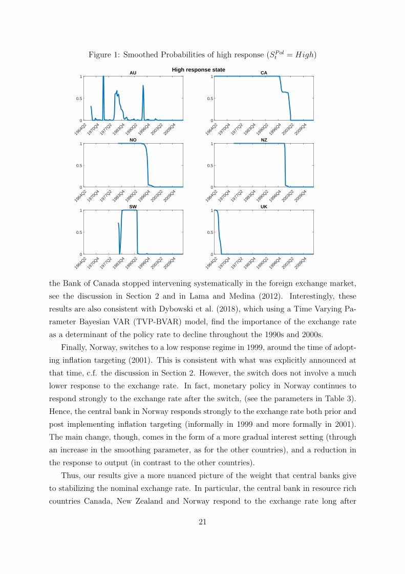
Figure 1: Smoothed Probabilities of high response (SPolt = High)

1964

Q2

1970

Q4

1977

Q2

1983

Q4

1990

Q2

1996

Q4

2003

Q2

2009

Q40

0.5

1AU

1964

Q2

1970

Q4

1977

Q2

1983

Q4

1990

Q2

1996

Q4

2003

Q2

2009

Q40

0.5

1CA

1964

Q2

1970

Q4

1977

Q2

1983

Q4

1990

Q2

1996

Q4

2003

Q2

2009

Q40

0.5

1NO

1964

Q2

1970

Q4

1977

Q2

1983

Q4

1990

Q2

1996

Q4

2003

Q2

2009

Q40

0.5

1NZ

1964

Q2

1970

Q4

1977

Q2

1983

Q4

1990

Q2

1996

Q4

2003

Q2

2009

Q40

0.5

1SW

1964

Q2

1970

Q4

1977

Q2

1983

Q4

1990

Q2

1996

Q4

2003

Q2

2009

Q40

0.5

1UK

High response state

the Bank of Canada stopped intervening systematically in the foreign exchange market,

see the discussion in Section 2 and in Lama and Medina (2012). Interestingly, these

results are also consistent with Dybowski et al. (2018), which using a Time Varying Pa-

rameter Bayesian VAR (TVP-BVAR) model, find the importance of the exchange rate

as a determinant of the policy rate to decline throughout the 1990s and 2000s.

Finally, Norway, switches to a low response regime in 1999, around the time of adopt-

ing inflation targeting (2001). This is consistent with what was explicitly announced at

that time, c.f. the discussion in Section 2. However, the switch does not involve a much

lower response to the exchange rate. In fact, monetary policy in Norway continues to

respond strongly to the exchange rate after the switch, (see the parameters in Table 3).

Hence, the central bank in Norway responds strongly to the exchange rate both prior and

post implementing inflation targeting (informally in 1999 and more formally in 2001).

The main change, though, comes in the form of a more gradual interest setting (through

an increase in the smoothing parameter, as for the other countries), and a reduction in

the response to output (in contrast to the other countries).

Thus, our results give a more nuanced picture of the weight that central banks give

to stabilizing the nominal exchange rate. In particular, the central bank in resource rich

countries Canada, New Zealand and Norway respond to the exchange rate long after

21

Figure 2: Smoothed Probabilities of high volatility (vol, 2)

1964

Q2

1970

Q4

1977

Q2

1983

Q4

1990

Q2

1996

Q4

2003

Q2

2009

Q40

0.5

1AU

1964

Q2

1970

Q4

1977

Q2

1983

Q4

1990

Q2

1996

Q4

2003

Q2

2009

Q40

0.5

1CA

1964

Q2

1970

Q4

1977

Q2

1983

Q4

1990

Q2

1996

Q4

2003

Q2

2009

Q40

0.5

1NO

1964

Q2

1970

Q4

1977

Q2

1983

Q4

1990

Q2

1996

Q4

2003

Q2

2009

Q40

0.5

1NZ

1964

Q2

1970

Q4

1977

Q2

1983

Q4

1990

Q2

1996

Q4

2003

Q2

2009

Q40

0.5

1SW

1964

Q2

1970

Q4

1977

Q2

1983

Q4

1990

Q2

1996

Q4

2003

Q2

2009

Q40

0.5

1UK

High volatility state

adopting inflation targeting, and for Norway, the response is high in all periods. These

are new findings in the literature. Australia stands our from the other resource rich

countries, as the interest rate responds to the exchange rate only at certain brief periods

early in the sample. However, as the Australia Dollar is the fifth most traded currency in

the world, responding to the exchange rate would be challenging, and could be the reason

for the lack of response. We emphasize, however, that we can not rule out that the central

banks that respond strongly to the exchange rate do so to achieve the inflation target

and overall macroeconomic stability. This may differ from country to country, based on

different preferences and concerns, see also Kam et al. (2009).

Our results stand in contrast to Lubik and Schorfheide (2007) and Dong (2013),

who analyse interest rate response in Australia, Canada, New Zealand and the U.K. In

particular, Lubik and Schorfheide (2007) found only Canada and UK to respond to the

exchange rate, while Dong (2013) found no evidence that the central Banks adjusted the

interest rate in response to the exchange rate. We believe that the added observables

in our setup, combined with realistic flexibilty that regime switching provides, allows for

better identification of parameters in more countries.

Turning to volatility in Figure 2, there is a striking similarity in the timing of the

switch between the high and low volatility regimes across countries, with the possible ex-

22

ception of Norway. In particular, independently of the chosen policy rules, the probability

of being in a regime of low volatility was high from the middle 1990s until the middle

2000s (the period referred to as ’the Great Moderation’). Following this, there is a high

probability of being in a high volatility regime during the period of the financial crisis in

all countries. For Australia, Canada and the UK for which we observe a longer sample,

there is an additional prolonged period of high volatility in the 1970s, whereas Norway

and Sweden experience a period of high volatility during the Nordic banking crisis in the

early 1990s. Norway also experience pronounced volatility in 2002/2003.

Hence, it seems that the switches in volatility indeed pick up well known episodes of

changes in exogenous volatility that many countries have in common, and independent

of the chosen regime.

6.3 Impulse responses

Having observed the different responses to the exchange rate, an interesting question to

discuss is the extent to which policy rules with a high response to the exchange rate

amplify or reduce the effects of terms of trade shocks on the domestic variables. To

address this, Figure 3 displays the generalized impulse responses to the terms-of-trade

shock (which increases export prices relative to import prices). The impulse responses

emphasize that responding strongly to the exchange rate will exacerbate the effects of a

terms-of-trade shock on both output and domestic inflation. In particular, a favorable

terms-of-trade shock appreciates the exchange rate on impact. The effect on output (and

inflation) will depend on the expected interest rate response. If the central bank is in a

policy regime of high interest rate response, then the exchange rate will appreciate by

much less, as the interest rate will also take into account the fact that the exchange rate

has appreciated. This will reverse the initial exchange rate response and push up output

and inflation relative to a regime of no exchange rate response. This is clearly seen in

Figure 3. Norway has been in a regime of high exchange rate response in most of the

sample, and the effect of the terms-of-trade shocks on output and inflation are therefore

clearly amplified relative to the other countries.

On a final note, recall from the discussion above that volatility of the terms of trade

is much higher in Australia, Canada, New Zealand, and in particular, Norway, than in

Sweden and the UK. This is most likely due to the fact that these are resource rich

countries, facing volatile commodity markets. Given this volatility, and a formal regime

of inflation targeting, it may seem surprising that the terms of trade shocks do not explain

even more of the variance in the nominal exchange rate than they do. The fact that the

23

Figure 3: Generalized IRFs to a Terms of trade shock

0 2 4 6 8 10 120

1

2

3

410-3 Output gap

0 2 4 6 8 10 12-1

0

1

2

3

4

5

610-3 Domestic Inflation

0 2 4 6 8 10 12-20

-15

-10

-5

0

510-3 Change in NEER

0 2 4 6 8 10 12-7

-6

-5

-4

-3

-2

-1

010-3 Interest rate

AUCANONZSWUK

IRF : Terms of trade shock shock

central banks have stabilized the exchange rate substantially more may have contributed

to this. As pointed out in Section 2, despite large differences in the terms of trade, the

exchange rate has about the same volatility across the countries in the recent period, but

with Australia at the higher end. Hence, we believe this suggests that monetary policy

has had a role to play in the stabilizing of the exchange rate (and subsequently inflation),

eventhough they have adopted inflation targeting.28

We conclude by noting that applying the same analysis across countries and yet getting

different results for the resource rich countries, is a strong indication that we are picking

up relevant information about changing regimes in open commodity exporting economies.

7 Extensions and robustness

In the figures above, we displayed the smoothed probabilities of being in various regimes

based on the mode. We believe our regime switching model suggests a reasonable pic-

ture of policy switches and spurs of volatility consistent with historical experience and

28Finally, the contributions to net capital outflows from high public sector foreign savings during high

oil-tax income periods, may also have helped contain nominal exchange rate appreciation, in particular

in Norway. This mechanism has allowed the policymakers to respond to the exchange rate.

24

information available from speeches and publication from the relevant Central Banks.

From Table 4, we saw that such a model was also preferred to a constant parameter or

volatility model. Still it is interesting to know what the results would have been if we

had allowed for different regime switching model, say allowing for switches in volatility

only or parameter only.

Table 5 in Appendix B displays the coefficients in the policy rule for all countries

assuming a model that only allows for switches in volatility (only) The table confirms

again that Norway responds by far the most to the exchange rate, followed by New

Zealand, while there is virtually no response to the exchange rate in the other countries.

This is very similar to the constant parameter case. Also, as in the constant parameter

model, there is very little response to inflation and a high response to output (except

Norway). Smoothing is also high in all countries. This could suggest that the model now

interprets some of the periods of known policy changes as spurs of high volatility instead.

Table 6 in Appendix B displays the coefficients in the policy rule for all countries

assuming a model that only allows for switches in parameters (only). Compared to the

constant parameter and volatility only model, now also Canada and the UK respond,

in addition to Norway and New Zealand. We also see that the interest rate generally

respond more to inflation and output when we allow parameters to also change.

The sample start used in the estimation varies, with data dating back to the 1960s

for all countries but Norway and Sweden, that has data only available from the 1980s.

To examine the results starting in more recent time for all countries, we start the sample

in 1980 also for Australia, Canada, New Zealand and the UK. Re-estimating the model

from 1980, we find the overall conclusion to be robust. In particular, Canada switches

between high and low response as before, although for some countries, Canada and the

UK in particular, the switches have moved a few quarters relative to the baseline model,

see the Figure 5 in the Appendix.

8 Conclusion

We analyse whether inflation targeting central banks in advanced small open economies

respond to the exchange rate. Using a Markov switching DSGE model that explicitly al-

lows for parameter changes, we observe that the size of policy responses and the volatility

of structural shocks, have not remained constant during the sample period.

Our results give a more nuanced picture of the weight that central banks give to

stabilizing the nominal exchange rate. In particular, while the central banks in Sweden

25

and the UK switch to a low exchange rate response regime shortly after severe periods

of currency crisis and collapse of their fixed exchange rate regime, the central bank in

Canada, New Zealand and Norway continue to respond to the exchange rate even after

adopting inflation targeting framework, and for Norway, throughout the whole sample.

Australia stands out from the other resource rich countries, by responding to the exchange

rate only at certain brief periods early in the sample.

Through our Markov Switching mechanism we are able to compare the estimated effect

of shocks, across different types of monetary policy regimes, and across countries where

export is important to a varying degree. Thus, the fact that we are applying the same

analysis across small open economies and yet get different results for the various countries,

is a strong indication that we are picking up relevant information about changing regimes

in open economies.

26

References

Alstadheim, R. (2016). Exchange rate regimes in Norway 1816-2016. Staff memo no. 15,

Norges Bank.

Bjørnland, H. C. (2009). Monetary policy and exchange rate overshooting: Dornbusch

was right after all. Journal of International Economics 79 (1), 64–77.

Bjørnland, H. C. and J. I. Halvorsen (2014). How does monetary policy respond to

exchange rate movements? new international evidence. Oxford Bulletin of Economics

and Statistics 76 (2), 208–232.

Bjørnland, H. C., V. H. Larsen, and J. Maih (2018). Oil and macroeconomic (in) stability.

American Economic Journal: Macroeconomics 10 (4), 128–51.

Bordo, M. D., A. Redish, and R. A. Shearer (1999). Canada’s Monetary System in

Historical Perspective: Two faces of the exchange rate regime. Discussion Paper 24,

Department of Economics, The University of British Columbia.

Brooks, R., K. Rogoff, A. Mody, N. Oomes, and A. M. Husain (2004). Evolution and

Performance of Exchange Rate Regimes. IMF Occasional Papers 229, International

Monetary Fund.

Calvo, G. A. and C. M. Reinhart (2002). Fear of floating. The Quarterly Journal of

Economics 117 (2), 379–408.

Canova, F., F. Ferroni, and C. Matthes (2014). Choosing The Variables To Estimate

Singular DSGE Models. Journal of Applied Econometrics 29 (7), 1099–1117.

Caputo, R. and L. O. Herrera (2017). Following the leader? the relevance of the fed funds

rate for inflation targeting countries. Journal of International Money and Finance 71,

25–52.

Catao, L. and R. Chang (2013). Monetary Rules for Commodity Traders. IMF Economic

Review 61 (1), 52–91.

Christiano, L. J., M. Trabandt, and K. Walentin (2011). DSGE models for monetary

policy. In B. Friedman and M. Woodford (Eds.), Handbook of Monetary Economics,

Volume 3A, pp. 285–367. Elsevier.

Clarida, R., J. Galı, and M. Gertler (1998). Monetary policy rules in practice: some

international evidence. European Economic Review 42 (6), 1033–1067.

27

Corsetti, G., L. Dedola, and S. Leduc (2010). Optimal monetary policy in open economies.

In B. M. Friedman and M. Woodford (Eds.), Handbook of Monetary Economics, Vol-

ume 3 of Handbook of Monetary Economics, Chapter 16, pp. 861–933. Elsevier.

De Paoli, B. (2009). Monetary policy and welfare in a small open economy. Journal of

International Economics 77 (1), 11–22.

Debelle, G. (2018). Twenty-five years of inflation targeting in Australia. Speech, Reserve

Bank of Australia.

Del Negro, M. and F. Schorfheide (2009). Inflation dynamics in a small open economy

model under inflation targeting: Some evidence from Chile. Central Banking, Analysis,

and Economic Policies Book Series 13, 511–562.

Dong, W. (2013). Do central banks respond to exchange rate movements? Some new

evidence from structural estimation. Canadian Journal of Economics 46 (2), 555–586.

Dybowski, T. P., M. Hanisch, and B. Kempa (2018). The role of the exchange rate

in Canadian monetary policy: evidence from a TVP-BVAR model. Empirical Eco-

nomics 55 (2), 471–494.

Engel, C. (2014). Exchange Rates and Interest Parity, Volume 4 of Handbook of Interna-

tional Economics, Chapter 0, pp. 453–522. Elsevier.

Engel, C. and K. West (2006). Taylor Rules and the Deutschmark-Dollar Real Exchange

Rate. Journal of Money, Credit and Banking 38 (5), 1175–1194.

Evans, M. D. (1996). 21 peso problems: Their theoretical and empirical implications.

In Statistical Methods in Finance, Volume 14 of Handbook of Statistics, pp. 613 – 646.

Elsevier.

Farmer, R. E., D. F. Waggoner, and T. Zha (2011). Minimal state variable solutions to

markov-switching rational expectations models. Journal of Economic Dynamics and

Control 35 (12), 2150–2166.

Galı, J. and T. Monacelli (2005). Monetary policy and exchange rate volatility in a small

open economy. Review of Economic Studies 72, 707–734.

Gelman, A., J. B. Carlin, H. S. Stern, and D. B. Rubin (2004). Bayesian Data Analysis

(2 ed.). Chapman & Hall/CRC.

28

Ghosh, A. R., J. D. Ostry, and M. S. Qureshi (2015). Exchange Rate Management and

Crisis Susceptibility: A Reassessment. IMF Economic Review 63 (1), 238–276.

Ilzetzki, E., C. M. Reinhart, and K. S. Rogoff (2017a). Exchange arrangements entering

the 21st century: Which anchor will hold? Working Paper 23134, National Bureau of

Economic Research.

Ilzetzki, E., C. M. Reinhart, and K. S. Rogoff (2017b). The Country Chronologies to

Exchange Rate Arrangements into the 21st Century: Will the Anchor Currency Hold?

Working Papers 23135, National Bureau of Economic Research, Inc.

Jin, H. and C. Xiong (2020). Fiscal stress and monetary policy stance in oil-exporting

countries. Journal of International Money and Finance 111.

Kam, T., K. Lees, and P. Liu (2009). Uncovering the hit list for small inflation targeters:

A bayesian structural analysis. Journal of Money, Credit and Banking 41 (4), 583–618.

Karaboga, D. and B. Akay (2011). A Modified Artificial Bee Colony (ABC) Algorithm

for Constrained Optimization Problems. Appl. Soft Comput. 11 (3), 3021–3031.

Kim, C.-J. and C. R. Nelson (1999). Has the U.S. economy become more stable? A

bayesian approach based on a markov-switching model of the business cycle. The

Review of Economics and Statistics 81 (4), 608–616.

Klein, M. W. and J. C. Shambaugh (2012). Exchange Rate Regimes in the Modern Era,

Volume 1 of MIT Press Books. The MIT Press.

Lama, R. and J. P. Medina (2012). Is Exchange Rate Stabilization an Appropriate Cure

for the Dutch Disease? International Journal of Central Banking 8 (1), 5–46.

Liu, P. and H. Mumtaz (2011). Evolving macroeconomic dynamics in a small open

economy: An estimated markov switching dsge model for the uk. Journal of Money,

Credit and Banking 43 (7), 1443–1474.

Lubik, T. A. and F. Schorfheide (2004). Testing for indeterminacy: an application to US

monetary policy. American Economic Review 94 (1), 190–217.

Lubik, T. A. and F. Schorfheide (2007). Do Central Banks respond to exchange rate

movements? A structural investigation. Journal of Monetary Economics 54, 1069–

1087.

29

Maih, J. (2015). Efficient perturbation methods for solving regime-switching DSGE mod-

els. Norges Bank Working Paper Series 1/2015.

McDermott, J. and R. Williams (2018). Inflation targeting in New Zealand: an experience

in evolution. Speech, Reserve Bank of New Zealand.

Miasojedow, B., E. Moulines, and M. Vihola (2012). Adaptive parallel tempering algo-

rithm. ArXiv e-prints .

Mundell, R. A. (1963). Capital mobility and stabilization policy under fixed and flexible

exchange rates. The Canadian Journal of Economics and Political Science / Revue

canadienne d’Economique et de Science politique 29 (4), 475–485.

Obstfeld, M. and K. Rogoff (1995). The Mirage of Fixed Exchange Rates. Journal of

Economic Perspectives 9 (4), 73–96.

Reinhart, C. M. and K. S. Rogoff (2004). The Modern History of Exchange Rate Ar-

rangements: A Reinterpretation. The Quarterly Journal of Economics 119 (1), 1–48.

Rey, H. (2016). International Channels of Transmission of Monetary Policy and the

Mundellian Trilemma. Working Papers 21852, National Bureau of Economic Research,

Inc.

Scholl, A. and H. Uhlig (2008). New evidence on the puzzles: Results from agnostic

identification on monetary policy and exchange rates. Journal of International Eco-

nomics 76 (1), 1–13.

Sims, C. A. and T. Zha (2006). Where there regime switches in U.S. monetary policy?

American Economic Review 96 (1), 54–81.

Smets, F. and R. Wouters (2007). Shocks and frictions in us business cycles: A bayesian

DSGE approach. American Economic Review 97 (3), 586–606.

Stock, J. H. and M. W. Watson (2005). Understanding changes in international business

cycle dynamics. Journal of the European Economic Association 3 (5), 968–1006.

Svensson, L. E. O. and N. Williams (2007). Monetary policy with model uncertainty:

Distribution forecast targeting. CEPR Discussion Papers 6331, C.E.P.R.

Taylor, J. B. (2001). The role of the exchange rate in monetary-policy rules. The American

Economic Review 91 (2), 263–267.

30

Appendices

Appendix A Data and sources

We use nominal effective exchange rates from the BIS for all countries, based on their

time-varying narrow weight set. The data set is monthly and is downloaded from the

FRED database.29 From this we calculate quarterly averages. We invert the indexes so

that a higher index value indicates a weaker local currency.

Seasonally adjusted CPI series are collected from national sources (Australian Bureau of

Statistics, Statistics Canada, Statistics New Zealand, Statistics Norway, Statistics Swe-

den and Statistics UK) for all countries. We use standard series that are long enough for

our sample: For Australia and Canada we use Consumer Prices, All Items, for Sweden we

use the Consumer Price Index, Standardized, for New Zealand we use Consumer Prices

All Groups, for Norway we use Consumer Prices, All Items, Total and for the UK, we use

the All Items Retail Price Index. The data series are monthly. From this we calculate

quarterly averages.30

For real GDP, we use data from national sources, except for Canada, where we use

data from the IMF IFS and for New Zealand where we use data from OECD in order

to get long enough series.31 The data series are seasonally adjusted by their national

sources, except for Canada and Sweden, where we have to seasonally adjust the data.

For interest rates, we collect three-month interbank rates for Australia, Canada, Swe-

den, New Zealand and the UK from the FRED database. The interest rate for Norway

was downloaded from national sources via Datastream.32 National sources did not pro-

vide long enough series for the other three countries.

29We use the following FRED data series Australia: NNAUBIS, New Zealand: NNNZBIS, Canada:

NNCABIS, UK: NNGBBIS, Norway: NNNOBIS and Sweden: NNSEBIS.30Datastream series ID AUCONPRCF for Australia, UKCHAW for the UK, CNCONPRCF for Canada,

SDCCPI..E for Sweden, NZCONPRCF for New Zealand and NWCONPRCE for Norway.31EcoWin codes gbr01020 for the UK, swe01850 for Sweden and nor01005 for Norway, and Datas-

tream series AUGDP...D for Australia. The series for Canada collected from the IMF IFS is denoted

15699BVRZF..., and the OECD EO series for New Zealand is Q.NZL.GDPV32FRED data series are denoted Australia: IRTIBO1AUQ156N, Canada: IR3TIB01CAQ156N, Sweden:

IR3TIB01SEQ156N, New Zealand: IRTIBO1NZQ156N and the UK: IR3TTS01GBQ156N. For Norway,

we find the series in Datastream denoted: NWIBK3M.

31

For the terms of trade, we use data from national sources for Australia, Canada, New

Zealand and Norway33, while we use IMF-data for the UK and Sweden, in order to obtain

long enough data series for those countries.34

We construct series for foreign inflation and foreign GDP for each country, based on

time-varying weights from the BIS (the same set that was used to construct the effective

exchange rates). We select the three largest trading partners for each country from the

weight-set in the year 1993, and apply the time-varying weights to those three countries

(rescaled to make up 100 percent in total for each year). Weights are fixed back in time

from 1991, since the time-varying weights are available only from 1991. For most of the

sample, the three largest trading partners are, for Australia: the US, Japan and the Euro

Area, for New Zealand Australia, Japan and the US, for Norway: the Euro Area, Sweden

and the UK, for Canada: the US, Japan and the Euro area, for Sweden: the Euro area,

the US and the UK and for the UK: the Euro area, the US and Japan.35

33For Australia from Australian Bureu of Statistics via Datastream: AUTERMTDE, For Canada from

Statistics Canada via Datastream: CNTRMTRDG. The series from Statistics Canada is available back

to Q1 1981, and we use data from the OECD MEI before that. The two series track each other closely

after 1981. For New Zealand we use NZTOTPRCF from Datastream. For Norwegian terms of trade, we

use the series QUA PXM from Statistics Norway.34We calculate the terms of trade from IMF-data as the quarterly export price index divided by the

quarterly import price index (both unadjusted). The series IDs in the IMF IFS data base are, for e.g.

UK export prices, Q11276ZF. National series and IMF-series track each other closely for the UK and

Sweden.35Note that Euro area GDP/CPI series are only available from 1995/1996. To construct Euro area data

prior to 1995/1996, we construct time series based on data from Germany and France (weights 0.5 on

each in 1960). Inflation data for France, Germany, the Euro Area, the US and Japan are collected from

Datastream (local sources, corresponding to those for our six home countries under study). GDP data for

France, the Euro Area and the US are Ecowin-series, local sources (fra01980, emu01718, usa01006), while

GDP data for Germany (Q13499BURZF...) and Japan (Q15899BURZF...) are from IMF-IFS. Note also

that in calculating the foreign series for Australia and New Zealand, Japan has a more significant weight

than in the case of the other countries (where the weight is small or zero). The IMF IFS-series for

Japan, for the period before 1979:q3, is replaced with OECD EO-series QJPN.GDPV because the IMF

IFS-series seems to have a break and be non SA for the earlier period. This matters for Australia and

New Zealand where the weight for Japan is significant.

32

Appendix B Extra tables and figures

Table 4: Model comparison - Log MDD (Laplace)

AU CA NO NZ SW UK

Constant 3683.5 4469.7 2616.0 3194.1 2796.0 4253.1

Parameter only 3506.7 4384.9 2536.4 3207.4 2850.5 4285.9

Volatility only NaN 4443.4 2612.2 3237.1 2899.5 4385.7

Parameter and volatility 3773.9 4513.8 2793.0 3247.1 2942.6 4571.6

Table 5: Prior and poster mode, volatility only

Params P.distr P.prob low high AU CA NO NZ SW UK

ρi beta 0.90 0.40 0.75 0.89 0.89 0.95 0.92 0.87 0.92

γπ gamma 0.90 0.90 3.00 0.14 0.28 0.49 0.57 0.09 0.28

γy gamma 0.90 0.10 3.00 2.93 4.87 0.08 0.59 1.25 4.70

γe gamma 0.90 0.05 3.00 0.01 0.08 2.71 0.64 0.00 0.01

Table 6: Priors and Posterior mode, parameter only

Params P.distr P.prob low high AU CA NO NZ SW UK

ρi(SPolt = Low) beta 0.90 0.40 0.75 0.66 0.93 0.92 0.86 0.92 0.88

ρi(SPolt = High) beta 0.90 0.40 0.75 0.78 0.85 0.87 0.91 0.48 0.67

γπ(SPolt = Low) gamma 0.90 0.90 3.00 1.11 0.97 0.52 0.58 1.09 0.57

γπ(SPolt = High) gamma 0.90 0.90 3.00 0.15 0.56 0.52 0.58 1.09 0.57

γy(SPolt = Low) gamma 0.90 0.10 3.00 0.30 0.54 0.65 0.19 1.12 0.20

γy(SPolt = High) gamma 0.90 0.10 3.00 2.91 0.25 0.35 0.04 0.58 0.23

γe(SPolt = Low) gamma 0.90 0.05 3.00 0.00 0.06 1.26 0.00 0.00 0.10

γe(SPolt = High) gamma 0.90 0.05 3.00 0.02 0.43 2.39 1.45 0.00 1.22

33

Figure 4: Smoothed probabilities, high volatility (vol, 2) - volatility only

1964

Q2

1970

Q4

1977

Q2

1983

Q4

1990

Q2

1996

Q4

2003

Q2

2009

Q40

0.5

1AU

1964

Q2

1970

Q4

1977

Q2

1983

Q4

1990

Q2

1996

Q4

2003

Q2

2009

Q40

0.5

1CA

1964

Q2

1970

Q4

1977

Q2

1983

Q4

1990

Q2

1996

Q4

2003

Q2

2009

Q40

0.5

1NO

1964

Q2

1970

Q4

1977

Q2

1983

Q4

1990

Q2

1996

Q4

2003

Q2

2009

Q40

0.5

1NZ

1964

Q2

1970

Q4

1977

Q2

1983

Q4

1990

Q2

1996

Q4

2003

Q2

2009

Q40

0.5

1SW

1964

Q2

1970

Q4

1977

Q2

1983

Q4

1990

Q2

1996

Q4

2003

Q2

2009

Q40

0.5

1UK

High volatility state

34

Figure 5: High response: Smoothed probabilities - short sample (post 1980)

1980Q1 1984Q3 1989Q1 1993Q3 1998Q1 2002Q3 2007Q1 2011Q30

0.005

0.01UK

1980Q1 1984Q3 1989Q1 1993Q3 1998Q1 2002Q3 2007Q1 2011Q30

0.5

1CA

1980Q1 1984Q3 1989Q1 1993Q3 1998Q1 2002Q3 2007Q1 2011Q30

0.5

1AU

1980Q1 1984Q3 1989Q1 1993Q3 1998Q1 2002Q3 2007Q1 2011Q3

0.44

0.46

0.48NZ

Prob. of high exchange rate response

35

BI Norwegian Business SchoolCentre for Applied Macro - Petroleum economics (CAMP)N-0442 Oslo

www.bi.no/camp

CAMP Working Paper SeriesISSN: 1892-2198

Centre for Applied Macroeconomics and Commodity Prices (CAMP) will bring together economists working on applied macroeconomic issues, with specialemphasis on petroleum economics.

CENTRE FOR APPLIED MACROECONOMICS AND COMMODITY PRICES (CAMP)