dna mapping and brute force algorithms - phillip...
TRANSCRIPT

www.bioalgorithms.info An Introduction to Bioinformatics Algorithms
DNA Mapping and Brute Force Algorithms
An Introduction to Bioinformatics Algorithms www.bioalgorithms.info
1. Restriction Enzymes 2. Gel Electrophoresis 3. Partial Digest Problem 4. Brute Force Algorithm for Partial Digest Problem 5. Branch and Bound Algorithm for Partial Digest Problem
Outline

An Introduction to Bioinformatics Algorithms www.bioalgorithms.info
Section 1: Restriction Enzymes

An Introduction to Bioinformatics Algorithms www.bioalgorithms.info
Discovery of Restriction Enzymes
• HindII: First restriction enzyme. • Was discovered accidentally in 1970 while scientists were
studying how the bacterium Haemophilus influenzae takes up DNA from the virus.
• Recognizes and cuts DNA at sequences: • GTGCAC • GTTAAC

An Introduction to Bioinformatics Algorithms www.bioalgorithms.info
Discovering Restriction Enzymes
Werner Arber
Werner Arber Discovered restriction enzymes
Daniel Nathans Pioneered the application of restriction for the construction of genetic maps
Hamilton Smith Showed that restriction enzyme cuts DNA in the middle of a specific sequence
My father has discovered a servant who serves as a pair of scissors. If a foreign king invades a bacterium, this servant can cut him in small fragments, but he does not do any harm to his own king. Clever people use the servant with the scissors to find out the secrets of the kings. For this reason my father received the Nobel Prize for the discovery of the servant with the scissors.”
Daniel Nathans’ daughter (from Nobel lecture)
Hamilton Smith Daniel Nathans

An Introduction to Bioinformatics Algorithms www.bioalgorithms.info
Molecular Scissors
Molecular Cell Biology, 4th edition

An Introduction to Bioinformatics Algorithms www.bioalgorithms.info
Restriction Enzymes: Common Recognition Sites
Molecular Cell Biology, 4th edition

An Introduction to Bioinformatics Algorithms www.bioalgorithms.info
• Recombinant DNA technology
• Cloning
• cDNA/genomic library construction
• DNA mapping
Uses of Restriction Enzymes

An Introduction to Bioinformatics Algorithms www.bioalgorithms.info
• A restriction map is a map showing positions of restriction sites in a DNA sequence.
• If DNA sequence is known then construction of restriction map is trivial exercise.
• In early days of molecular biology DNA sequences were often unknown.
• Biologists had to solve the problem of constructing restriction maps without knowing DNA sequences.
Restriction Maps
An Introduction to Bioinformatics Algorithms www.bioalgorithms.info
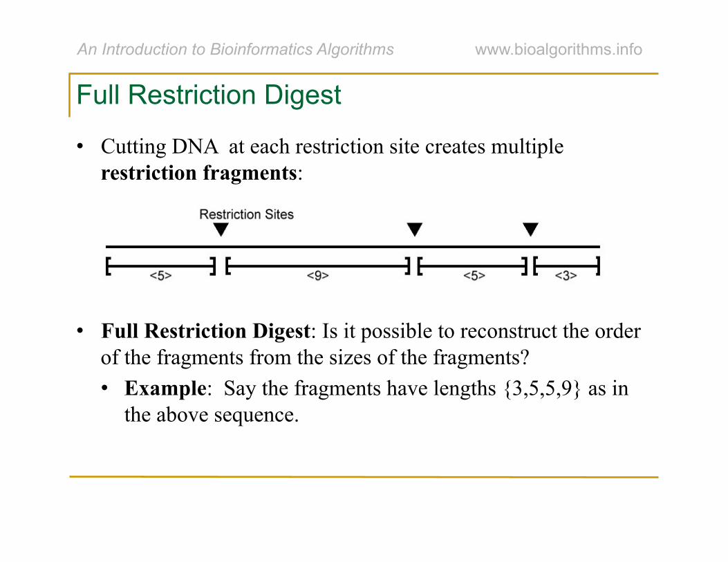
Full Restriction Digest
• Cutting DNA at each restriction site creates multiple restriction fragments:
• Full Restriction Digest: Is it possible to reconstruct the order of the fragments from the sizes of the fragments? • Example: Say the fragments have lengths {3,5,5,9} as in
the above sequence.
An Introduction to Bioinformatics Algorithms www.bioalgorithms.info
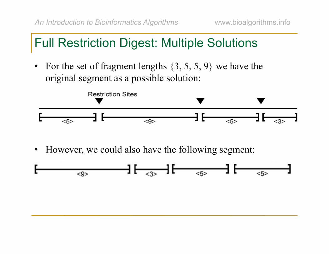
Full Restriction Digest: Multiple Solutions
• For the set of fragment lengths {3, 5, 5, 9} we have the original segment as a possible solution:
• However, we could also have the following segment:
An Introduction to Bioinformatics Algorithms www.bioalgorithms.info
Section 2: Gel Electrophoresis

An Introduction to Bioinformatics Algorithms www.bioalgorithms.info
• Restriction enzymes break DNA into restriction fragments.
• Gel electrophoresis: A process for separating DNA by size and measuring sizes of restriction fragments.
• Modern electrophoresis machines can separate DNA fragments that differ in length by 1 nucleotide for fragments up to 500 nucleotides long.
Gel Electrophoresis: Measure Segment Lengths

An Introduction to Bioinformatics Algorithms www.bioalgorithms.info
• DNA fragments are injected into a gel positioned in an electric field.
• DNA are negatively charged near neutral pH. • The ribose phosphate backbone of each nucleotide is
acidic; DNA has an overall negative charge. • Thus DNA molecules move towards the positive electrode.
Gel Electrophoresis: How It Works
An Introduction to Bioinformatics Algorithms www.bioalgorithms.info
Gel Electrophoresis
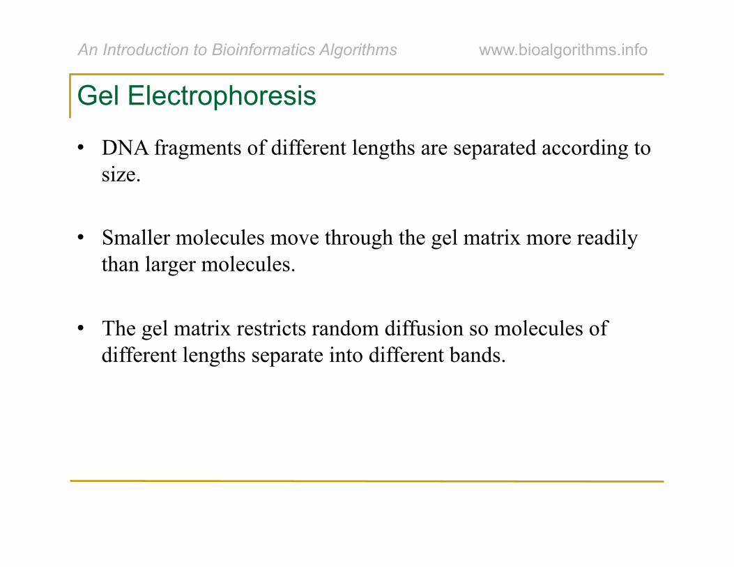
• DNA fragments of different lengths are separated according to size.
• Smaller molecules move through the gel matrix more readily than larger molecules.
• The gel matrix restricts random diffusion so molecules of different lengths separate into different bands.
An Introduction to Bioinformatics Algorithms www.bioalgorithms.info
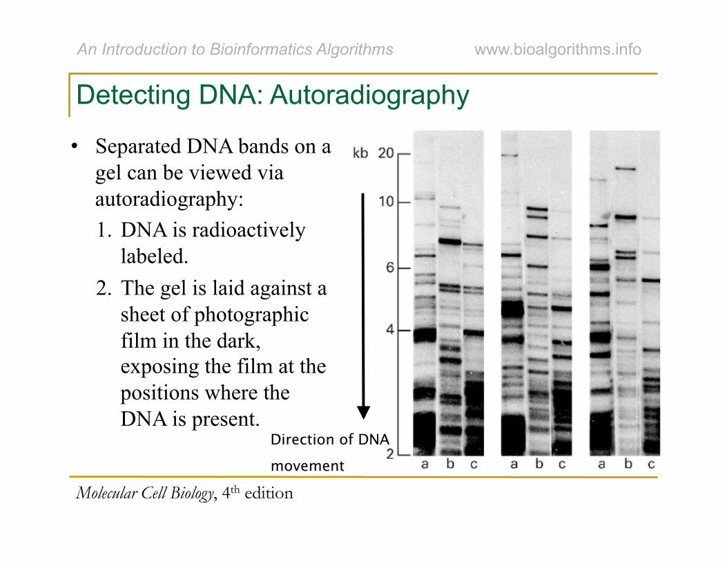
Direction of DNA movement
Detecting DNA: Autoradiography
• Separated DNA bands on a gel can be viewed via autoradiography: 1. DNA is radioactively
labeled. 2. The gel is laid against a
sheet of photographic film in the dark, exposing the film at the positions where the DNA is present.
Molecular Cell Biology, 4th edition
An Introduction to Bioinformatics Algorithms www.bioalgorithms.info
• Another way to visualize DNA bands in gel is through fluorescence: • The gel is incubated with a solution containing the
fluorescent dye ethidium. • Ethidium binds to the DNA. • The DNA lights up when the gel is exposed to ultraviolet
light.
Detecting DNA: Fluorescence

An Introduction to Bioinformatics Algorithms www.bioalgorithms.info
Section 3: Partial Digest Problem

An Introduction to Bioinformatics Algorithms www.bioalgorithms.info
• The sample of DNA is exposed to the restriction enzyme for only a limited amount of time to prevent it from being cut at all restriction sites; this procedure is called partial (restriction) digest.
• This experiment generates the set of all possible restriction fragments between every two (not necessarily consecutive) cuts.
• This set of fragment sizes is used to determine the positions of the restriction sites in the DNA sequence.
Partial Restriction Digest

An Introduction to Bioinformatics Algorithms www.bioalgorithms.info
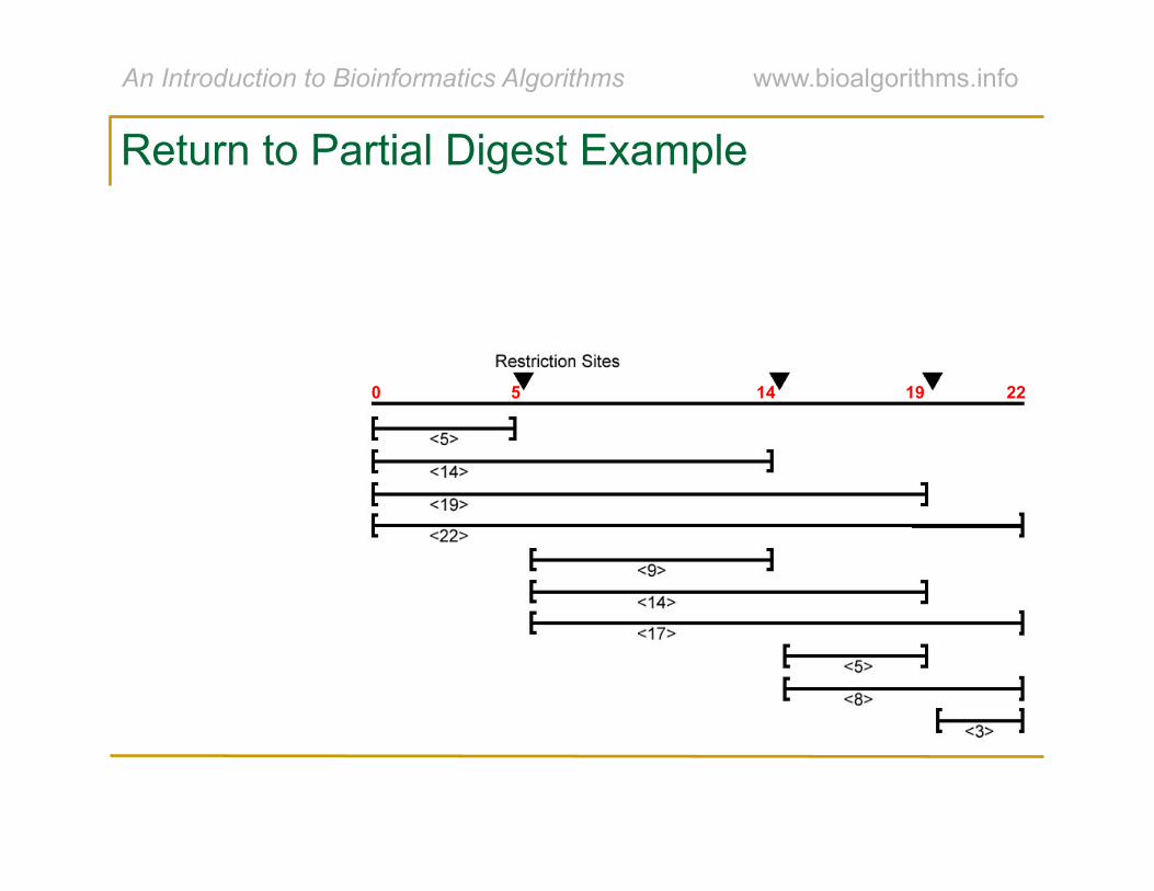
• Partial Digest results in the following 10 restriction fragments:
Partial Digest: Example
An Introduction to Bioinformatics Algorithms www.bioalgorithms.info
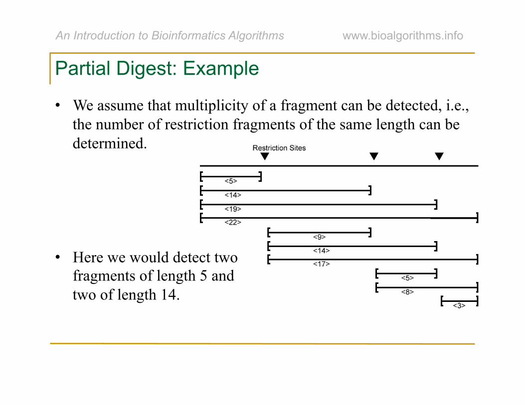
• We assume that multiplicity of a fragment can be detected, i.e., the number of restriction fragments of the same length can be determined.
• Here we would detect two fragments of length 5 and two of length 14.
Partial Digest: Example

An Introduction to Bioinformatics Algorithms www.bioalgorithms.info
Multiset: {3, 5, 5, 8, 9, 14, 14, 17, 19, 22}
Partial Digest: Example
• We therefore have a multiset of fragment lengths.
An Introduction to Bioinformatics Algorithms www.bioalgorithms.info
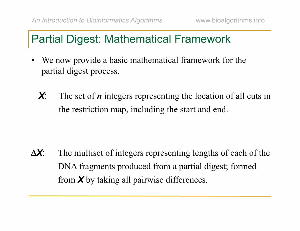
• We now provide a basic mathematical framework for the partial digest process.
The multiset of integers representing lengths of each of the DNA fragments produced from a partial digest; formed from X by taking all pairwise differences.
The set of n integers representing the location of all cuts in the restriction map, including the start and end.
X:
ΔX:
Partial Digest: Mathematical Framework

An Introduction to Bioinformatics Algorithms www.bioalgorithms.info
Return to Partial Digest Example
An Introduction to Bioinformatics Algorithms www.bioalgorithms.info
Return to Partial Digest Example
0 5 14 19 22

An Introduction to Bioinformatics Algorithms www.bioalgorithms.info
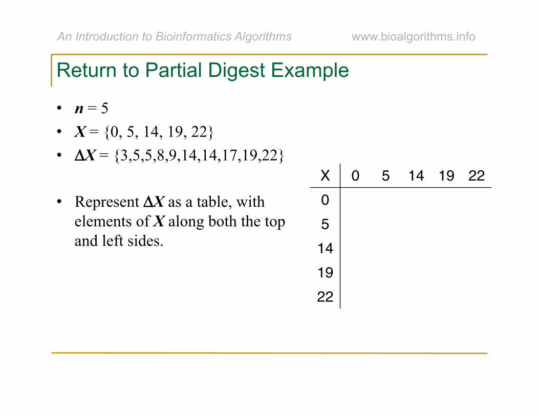
• n = 5
Return to Partial Digest Example
0 5 14 19 22

An Introduction to Bioinformatics Algorithms www.bioalgorithms.info
• n = 5 • X = {0, 5, 14, 19, 22}
Return to Partial Digest Example
0 5 14 19 22

An Introduction to Bioinformatics Algorithms www.bioalgorithms.info
Return to Partial Digest Example
0 5 14 19 22
• n = 5 • X = {0, 5, 14, 19, 22} • ΔX = {3,5,5,8,9,14,14,17,19,22}

An Introduction to Bioinformatics Algorithms www.bioalgorithms.info
• n = 5 • X = {0, 5, 14, 19, 22} • ΔX = {3,5,5,8,9,14,14,17,19,22}
• Represent ΔX as a table, with elements of X along both the top and left sides.
Return to Partial Digest Example
An Introduction to Bioinformatics Algorithms www.bioalgorithms.info
• n = 5 • X = {0, 5, 14, 19, 22} • ΔX = {3,5,5,8,9,14,14,17,19,22}
• Represent ΔX as a table, with elements of X along both the top and left sides.
X" 0" 5" 14" 19" 22"0"5"
14"19"22"
Return to Partial Digest Example

An Introduction to Bioinformatics Algorithms www.bioalgorithms.info
• n = 5 • X = {0, 5, 14, 19, 22} • ΔX = {3,5,5,8,9,14,14,17,19,22}
• Represent ΔX as a table, with elements of X along both the top and left sides.
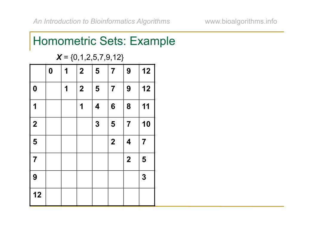
• We place xj – xi into entry (i,j) for all 1 ≤ i < j ≤ n
X" 0" 5" 14" 19" 22"0" 5" 14" 19" 22"5" 9" 14" 17"
14" 5" 8"19" 3"22"
Return to Partial Digest Example

An Introduction to Bioinformatics Algorithms www.bioalgorithms.info
• Goal: Given all pairwise distances between points on a line, reconstruct the positions of those points.
• Input: The multiset of pairwise distances L, containing n(n-1)/2 integers.
• Output: A set X, of n integers, such that ∆X = L.
Partial Digest Problem (PDP): Formulation

An Introduction to Bioinformatics Algorithms www.bioalgorithms.info
• It is not always possible to uniquely reconstruct a set X based only on ∆X. • Example: The sets
X = {0, 2, 5} (X + 10) = {10, 12, 15} both produce ∆X = ∆(X + 10) = {2, 3, 5} as their partial digest.
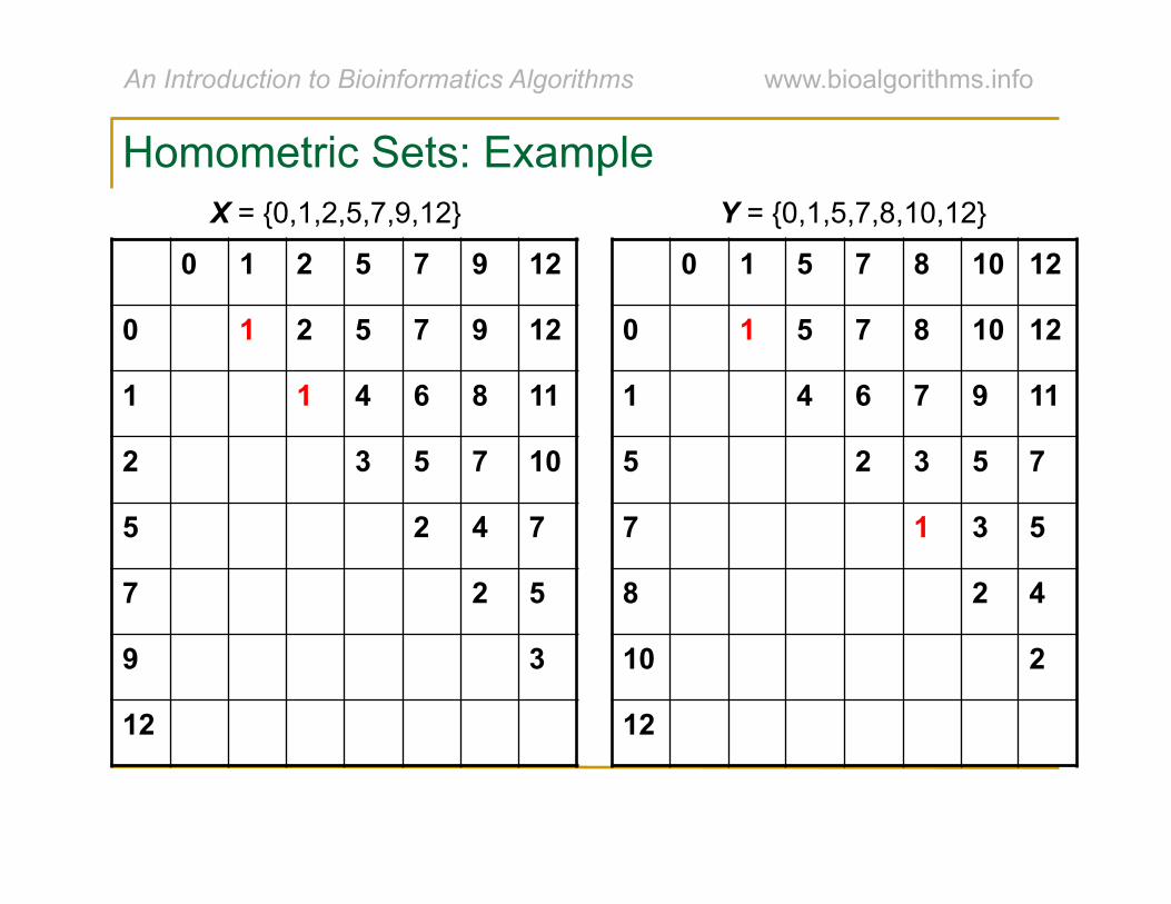
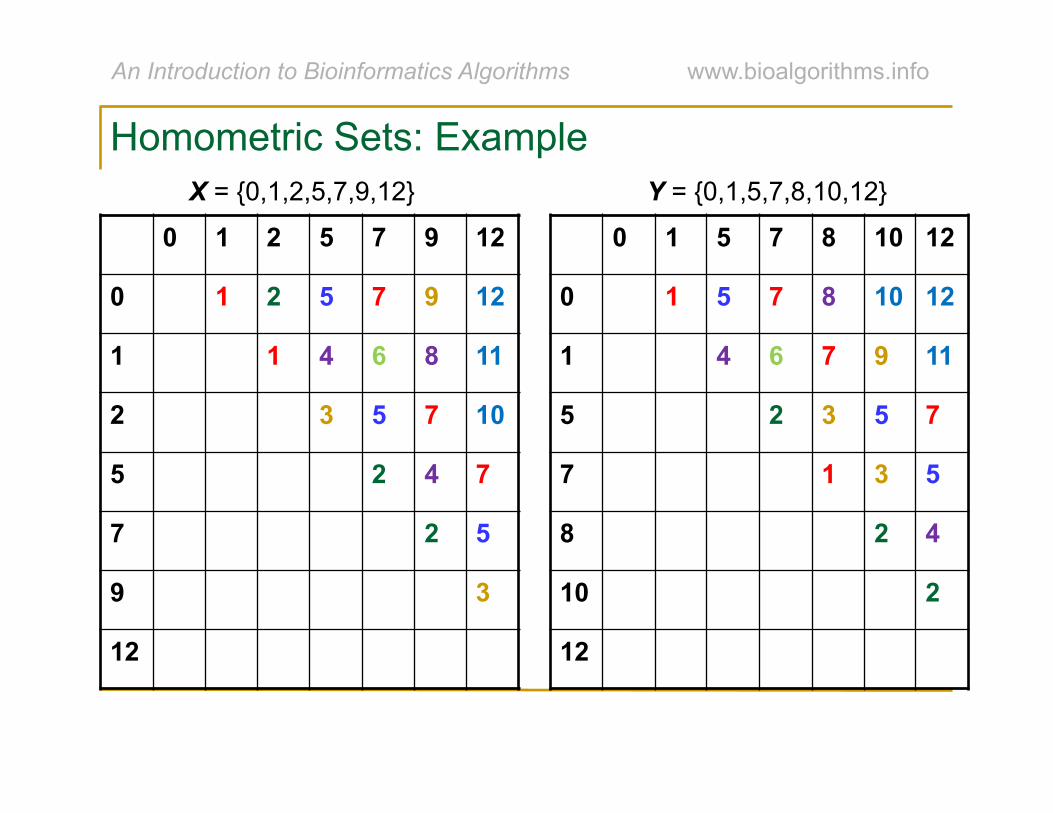
• Two sets X and Y are homometric if ∆X = ∆Y.
• The sets {0,1,2,5,7,9,12} and {0,1,5,7,8,10,12} present a less trivial example of homometric sets. They both digest into:
{1, 1, 2, 2, 2, 3, 3, 4, 4, 5, 5, 5, 6, 7, 7, 7, 8, 9, 10, 11, 12}
Multiple Solutions to the PDP

An Introduction to Bioinformatics Algorithms www.bioalgorithms.info
X = {0,1,2,5,7,9,12}
Homometric Sets: Example
An Introduction to Bioinformatics Algorithms www.bioalgorithms.info
0 1 2 5 7 9 12
0 1 2 5 7 9 12
1 1 4 6 8 11
2 3 5 7 10
5 2 4 7
7 2 5
9 3
12
X = {0,1,2,5,7,9,12}
Homometric Sets: Example

An Introduction to Bioinformatics Algorithms www.bioalgorithms.info
0 1 2 5 7 9 12
0 1 2 5 7 9 12
1 1 4 6 8 11
2 3 5 7 10
5 2 4 7
7 2 5
9 3
12
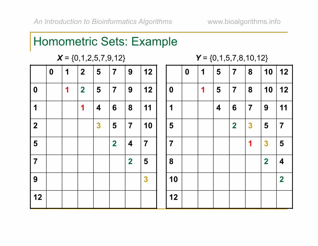
X = {0,1,2,5,7,9,12} Y = {0,1,5,7,8,10,12}
Homometric Sets: Example

An Introduction to Bioinformatics Algorithms www.bioalgorithms.info
0 1 2 5 7 9 12
0 1 2 5 7 9 12
1 1 4 6 8 11
2 3 5 7 10
5 2 4 7
7 2 5
9 3
12
0 1 5 7 8 10 12
0 1 5 7 8 10 12
1 4 6 7 9 11
5 2 3 5 7
7 1 3 5
8 2 4
10 2
12
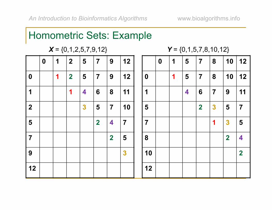
X = {0,1,2,5,7,9,12} Y = {0,1,5,7,8,10,12}
Homometric Sets: Example
An Introduction to Bioinformatics Algorithms www.bioalgorithms.info
0 1 2 5 7 9 12
0 1 2 5 7 9 12
1 1 4 6 8 11
2 3 5 7 10
5 2 4 7
7 2 5
9 3
12
0 1 5 7 8 10 12
0 1 5 7 8 10 12
1 4 6 7 9 11
5 2 3 5 7
7 1 3 5
8 2 4
10 2
12
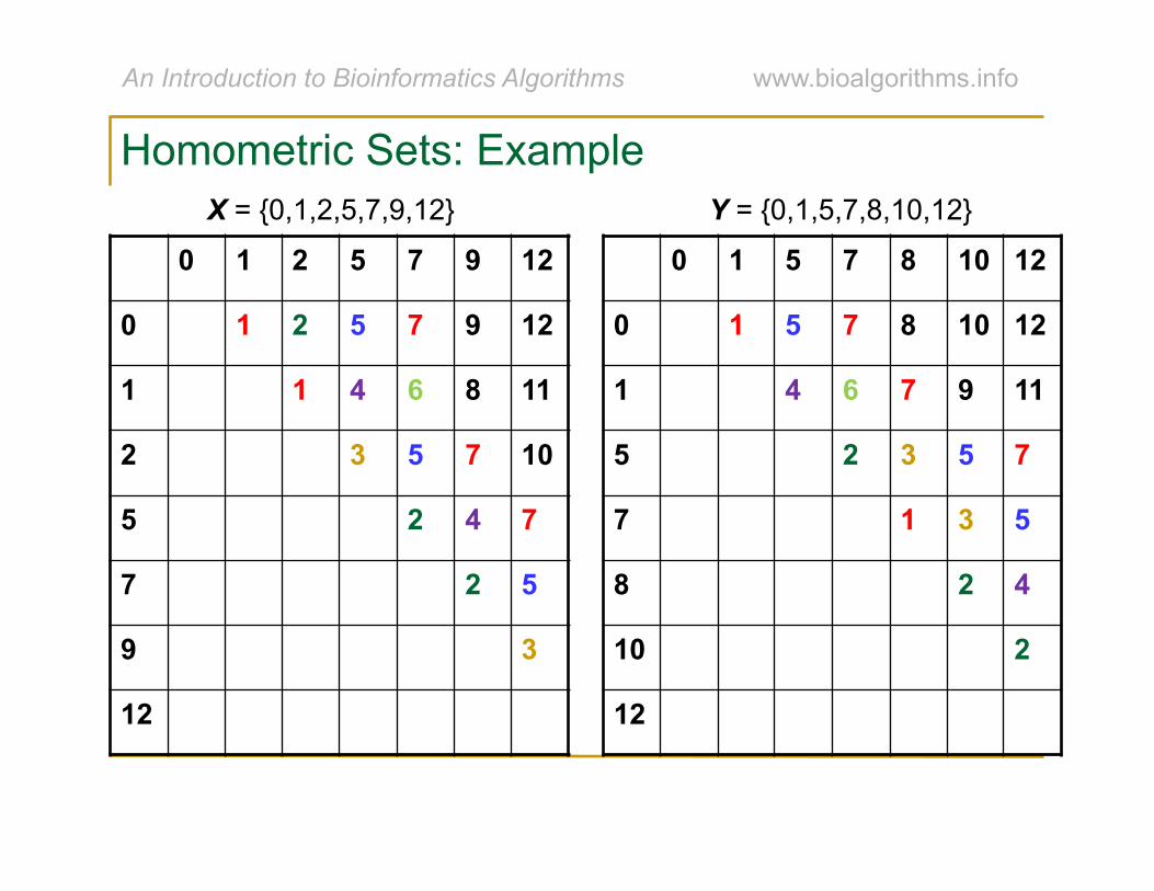
X = {0,1,2,5,7,9,12} Y = {0,1,5,7,8,10,12}
Homometric Sets: Example

An Introduction to Bioinformatics Algorithms www.bioalgorithms.info
0 1 2 5 7 9 12
0 1 2 5 7 9 12
1 1 4 6 8 11
2 3 5 7 10
5 2 4 7
7 2 5
9 3
12
0 1 5 7 8 10 12
0 1 5 7 8 10 12
1 4 6 7 9 11
5 2 3 5 7
7 1 3 5
8 2 4
10 2
12
X = {0,1,2,5,7,9,12} Y = {0,1,5,7,8,10,12}
Homometric Sets: Example
An Introduction to Bioinformatics Algorithms www.bioalgorithms.info
0 1 2 5 7 9 12
0 1 2 5 7 9 12
1 1 4 6 8 11
2 3 5 7 10
5 2 4 7
7 2 5
9 3
12
0 1 5 7 8 10 12
0 1 5 7 8 10 12
1 4 6 7 9 11
5 2 3 5 7
7 1 3 5
8 2 4
10 2
12
X = {0,1,2,5,7,9,12} Y = {0,1,5,7,8,10,12}
Homometric Sets: Example
An Introduction to Bioinformatics Algorithms www.bioalgorithms.info
0 1 2 5 7 9 12
0 1 2 5 7 9 12
1 1 4 6 8 11
2 3 5 7 10
5 2 4 7
7 2 5
9 3
12
0 1 5 7 8 10 12
0 1 5 7 8 10 12
1 4 6 7 9 11
5 2 3 5 7
7 1 3 5
8 2 4
10 2
12
X = {0,1,2,5,7,9,12} Y = {0,1,5,7,8,10,12}
Homometric Sets: Example

An Introduction to Bioinformatics Algorithms www.bioalgorithms.info
0 1 2 5 7 9 12
0 1 2 5 7 9 12
1 1 4 6 8 11
2 3 5 7 10
5 2 4 7
7 2 5
9 3
12
0 1 5 7 8 10 12
0 1 5 7 8 10 12
1 4 6 7 9 11
5 2 3 5 7
7 1 3 5
8 2 4
10 2
12
X = {0,1,2,5,7,9,12} Y = {0,1,5,7,8,10,12}
Homometric Sets: Example

An Introduction to Bioinformatics Algorithms www.bioalgorithms.info
0 1 2 5 7 9 12
0 1 2 5 7 9 12
1 1 4 6 8 11
2 3 5 7 10
5 2 4 7
7 2 5
9 3
12
0 1 5 7 8 10 12
0 1 5 7 8 10 12
1 4 6 7 9 11
5 2 3 5 7
7 1 3 5
8 2 4
10 2
12
X = {0,1,2,5,7,9,12} Y = {0,1,5,7,8,10,12}
Homometric Sets: Example
An Introduction to Bioinformatics Algorithms www.bioalgorithms.info
0 1 2 5 7 9 12
0 1 2 5 7 9 12
1 1 4 6 8 11
2 3 5 7 10
5 2 4 7
7 2 5
9 3
12
0 1 5 7 8 10 12
0 1 5 7 8 10 12
1 4 6 7 9 11
5 2 3 5 7
7 1 3 5
8 2 4
10 2
12
X = {0,1,2,5,7,9,12} Y = {0,1,5,7,8,10,12}
Homometric Sets: Example

An Introduction to Bioinformatics Algorithms www.bioalgorithms.info
0 1 2 5 7 9 12
0 1 2 5 7 9 12
1 1 4 6 8 11
2 3 5 7 10
5 2 4 7
7 2 5
9 3
12
0 1 5 7 8 10 12
0 1 5 7 8 10 12
1 4 6 7 9 11
5 2 3 5 7
7 1 3 5
8 2 4
10 2
12
X = {0,1,2,5,7,9,12} Y = {0,1,5,7,8,10,12}
Homometric Sets: Example

An Introduction to Bioinformatics Algorithms www.bioalgorithms.info
0 1 2 5 7 9 12
0 1 2 5 7 9 12
1 1 4 6 8 11
2 3 5 7 10
5 2 4 7
7 2 5
9 3
12
0 1 5 7 8 10 12
0 1 5 7 8 10 12
1 4 6 7 9 11
5 2 3 5 7
7 1 3 5
8 2 4
10 2
12
X = {0,1,2,5,7,9,12} Y = {0,1,5,7,8,10,12}
Homometric Sets: Example
An Introduction to Bioinformatics Algorithms www.bioalgorithms.info
0 1 2 5 7 9 12
0 1 2 5 7 9 12
1 1 4 6 8 11
2 3 5 7 10
5 2 4 7
7 2 5
9 3
12
0 1 5 7 8 10 12
0 1 5 7 8 10 12
1 4 6 7 9 11
5 2 3 5 7
7 1 3 5
8 2 4
10 2
12
X = {0,1,2,5,7,9,12} Y = {0,1,5,7,8,10,12}
Homometric Sets: Example
An Introduction to Bioinformatics Algorithms www.bioalgorithms.info
Section 4: Brute Force Algorithm for
Partial Digest Problem

An Introduction to Bioinformatics Algorithms www.bioalgorithms.info
• Brute force algorithms, also known as exhaustive search algorithms, examine every possible variant to find a solution.
• Efficient only in rare cases; usually impractical.
Brute Force Algorithms

An Introduction to Bioinformatics Algorithms www.bioalgorithms.info
1. Find the restriction fragment of maximum length M. Note: M is the length of the DNA sequence.
2. For every possible set X={0, x2, … ,xn-1, M}
compute the corresponding ΔX.
3. If ΔX is equal to the experimental partial digest L, then X is a possible restriction map.
Partial Digest: Brute Force

An Introduction to Bioinformatics Algorithms www.bioalgorithms.info
�
1 BruteForcePDP(L,n) :2 M← maximum element in L3 for every set of n integers 0 < x2 < < xn−1 < M
4 X← 0,x2,…xn−1,M{ }5 Form DX from X6 if DX = L7 return X8 output "no solution"
Partial Digest: Brute Force

An Introduction to Bioinformatics Algorithms www.bioalgorithms.info
• BruteForcePDP takes O(M n-2) time since it must examine all possible sets of positions. Note: the number of such sets is
• One way to improve the algorithm is to limit the values of xi to only those values which occur in L, because we are assuming for the sake of simplicity that 0 is contained in X.
Efficiency of BruteForcePDP

An Introduction to Bioinformatics Algorithms www.bioalgorithms.info
�
1 BruteForcePDP(L,n) :2 M← maximum element in L3 for every set of n integers 0 < x2 < < xn−1 < M
4 X← 0,x2,…xn−1,M{ }5 Form DX from X6 if DX = L7 return X8 output "no solution"
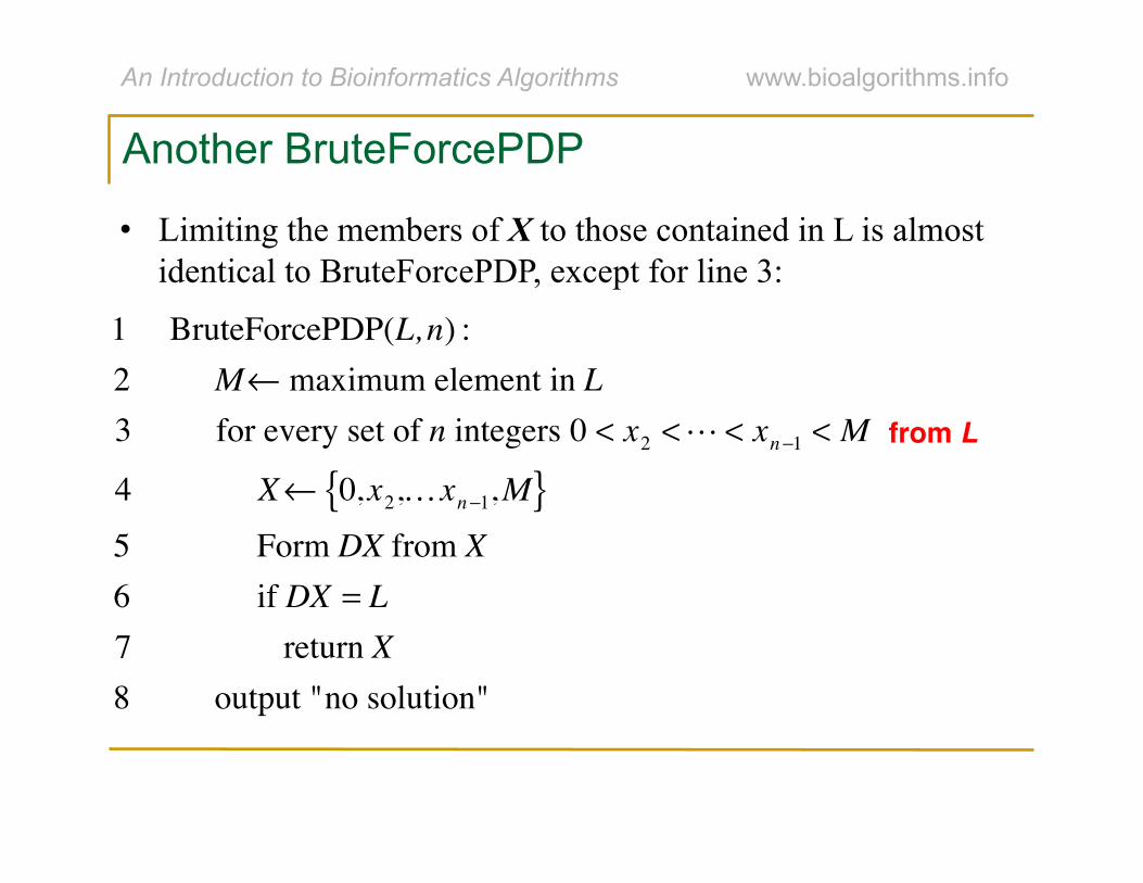
Another BruteForcePDP
• Limiting the members of X to those contained in L is almost identical to BruteForcePDP, except for line 3:
An Introduction to Bioinformatics Algorithms www.bioalgorithms.info
Another BruteForcePDP
• Limiting the members of X to those contained in L is almost identical to BruteForcePDP, except for line 3:
from L
�
1 BruteForcePDP(L,n) :2 M← maximum element in L3 for every set of n integers 0 < x2 < < xn−1 < M
4 X← 0,x2,…xn−1,M{ }5 Form DX from X6 if DX = L7 return X8 output "no solution"
An Introduction to Bioinformatics Algorithms www.bioalgorithms.info
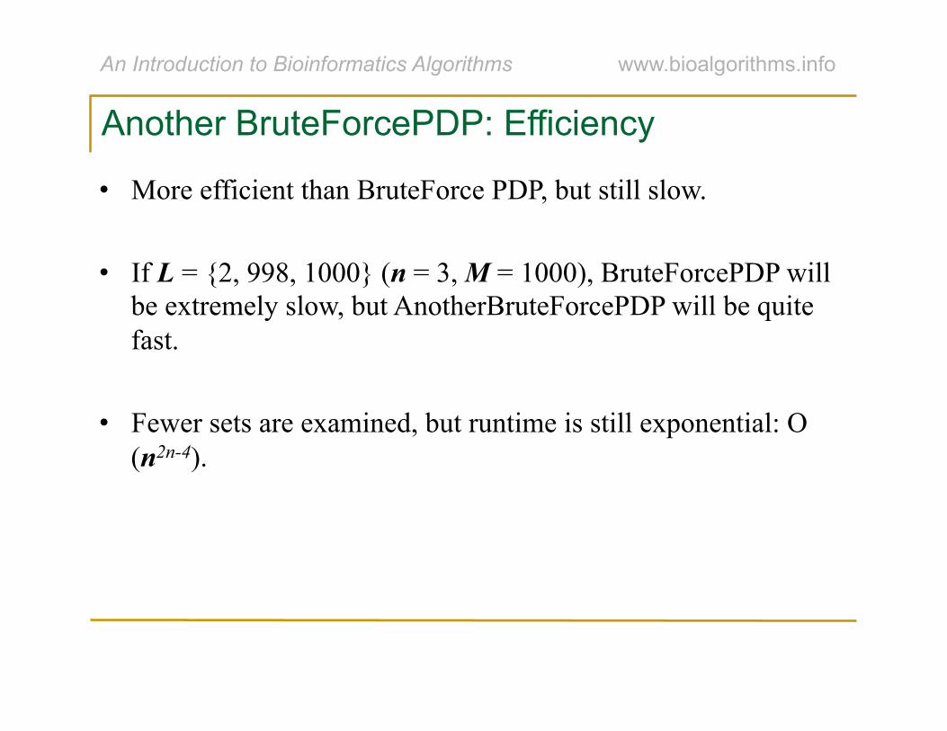
• More efficient than BruteForce PDP, but still slow.
• If L = {2, 998, 1000} (n = 3, M = 1000), BruteForcePDP will be extremely slow, but AnotherBruteForcePDP will be quite fast.
• Fewer sets are examined, but runtime is still exponential: O(n2n-4).
Another BruteForcePDP: Efficiency

An Introduction to Bioinformatics Algorithms www.bioalgorithms.info
Section 5: Branch and Bound Algorithm for Partial
Digest Problem
An Introduction to Bioinformatics Algorithms www.bioalgorithms.info
1. Begin with X = {0}.
Branch and Bound Algorithm for PDP
An Introduction to Bioinformatics Algorithms www.bioalgorithms.info
1. Begin with X = {0}. 2. Remove the largest element in L and place it in X.
Branch and Bound Algorithm for PDP
An Introduction to Bioinformatics Algorithms www.bioalgorithms.info
1. Begin with X = {0}. 2. Remove the largest element in L and place it in X. 3. See if the element fits on the right or left side of the restriction
map.
Branch and Bound Algorithm for PDP

An Introduction to Bioinformatics Algorithms www.bioalgorithms.info
1. Begin with X = {0}. 2. Remove the largest element in L and place it in X. 3. See if the element fits on the right or left side of the restriction
map. 4. When if fits, find the other lengths it creates and remove those
from L.
Branch and Bound Algorithm for PDP

An Introduction to Bioinformatics Algorithms www.bioalgorithms.info
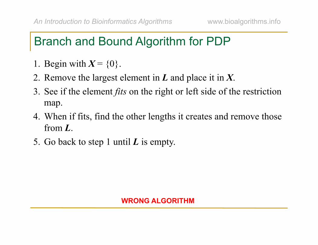
1. Begin with X = {0}. 2. Remove the largest element in L and place it in X. 3. See if the element fits on the right or left side of the restriction
map. 4. When if fits, find the other lengths it creates and remove those
from L. 5. Go back to step 1 until L is empty.
Branch and Bound Algorithm for PDP
An Introduction to Bioinformatics Algorithms www.bioalgorithms.info
1. Begin with X = {0}. 2. Remove the largest element in L and place it in X. 3. See if the element fits on the right or left side of the restriction
map. 4. When if fits, find the other lengths it creates and remove those
from L. 5. Go back to step 1 until L is empty.
Branch and Bound Algorithm for PDP
WRONG ALGORITHM

An Introduction to Bioinformatics Algorithms www.bioalgorithms.info
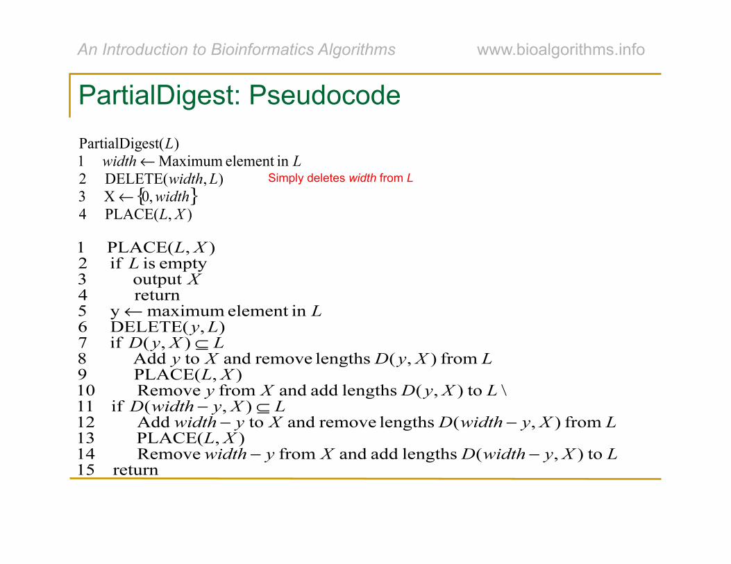
• Before describing PartialDigest, first define D(y, X) as the multiset of all distances between point y and all other points in the set X.
Defining D(y, X)
An Introduction to Bioinformatics Algorithms www.bioalgorithms.info
Simply deletes width from L
PartialDigest: Pseudocode

An Introduction to Bioinformatics Algorithms www.bioalgorithms.info
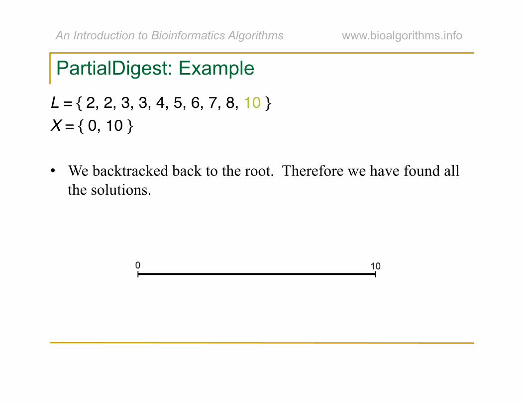
L = { 2, 2, 3, 3, 4, 5, 6, 7, 8, 10 }"X = { }"
PartialDigest: Example
An Introduction to Bioinformatics Algorithms www.bioalgorithms.info
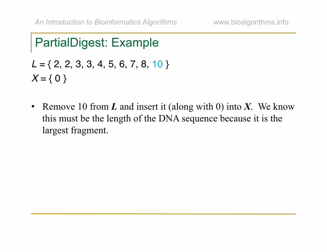
L = { 2, 2, 3, 3, 4, 5, 6, 7, 8, 10 }"X = { 0 }"
• Remove 10 from L and insert it (along with 0) into X. We know this must be the length of the DNA sequence because it is the largest fragment.
PartialDigest: Example
An Introduction to Bioinformatics Algorithms www.bioalgorithms.info
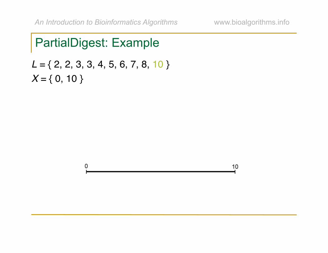
L = { 2, 2, 3, 3, 4, 5, 6, 7, 8, 10 }"X = { 0, 10 }"
PartialDigest: Example
An Introduction to Bioinformatics Algorithms www.bioalgorithms.info
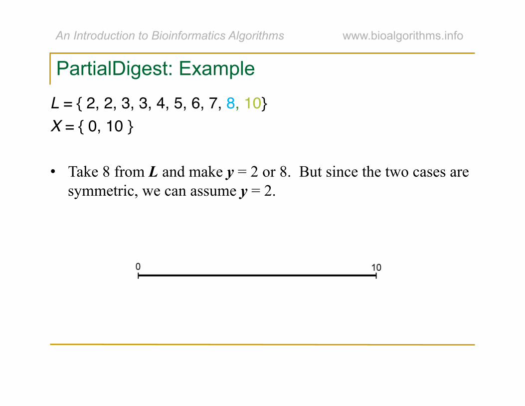
L = { 2, 2, 3, 3, 4, 5, 6, 7, 8, 10}"X = { 0, 10 }"
• Take 8 from L and make y = 2 or 8. But since the two cases are symmetric, we can assume y = 2.
PartialDigest: Example
An Introduction to Bioinformatics Algorithms www.bioalgorithms.info
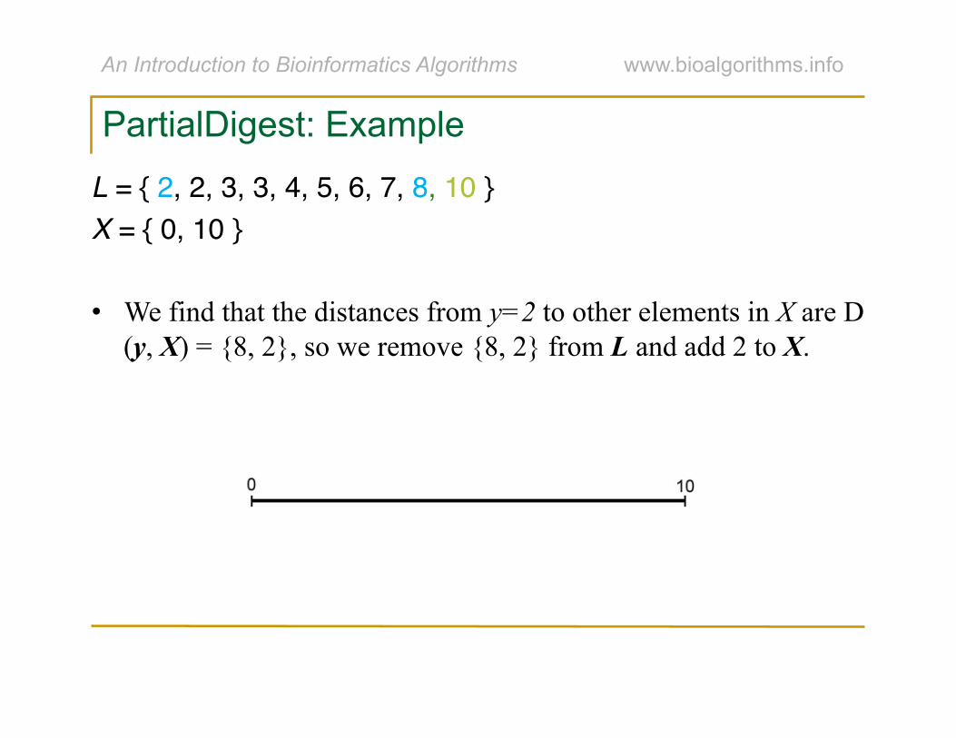
L = { 2, 2, 3, 3, 4, 5, 6, 7, 8, 10 }"X = { 0, 10 }"
• We find that the distances from y=2 to other elements in X are D(y, X) = {8, 2}, so we remove {8, 2} from L and add 2 to X.
PartialDigest: Example

An Introduction to Bioinformatics Algorithms www.bioalgorithms.info
L = { 2, 2, 3, 3, 4, 5, 6, 7, 8, 10 }"X = { 0, 2, 10 }"
PartialDigest: Example

An Introduction to Bioinformatics Algorithms www.bioalgorithms.info
L = { 2, 2, 3, 3, 4, 5, 6, 7, 8, 10 }"X = { 0, 2, 10 }"
• Take 7 from L and make y = 7 or y = 10 – 7 = 3. We will explore y = 7 first, so D(y, X ) = {7, 5, 3}.
PartialDigest: Example

An Introduction to Bioinformatics Algorithms www.bioalgorithms.info
L = { 2, 2, 3, 3, 4, 5, 6, 7, 8, 10 }"X = { 0, 2, 10 }"
• For y = 7 first, D(y, X ) = {7, 5, 3}. Therefore we remove {7, 5 ,3} from L and add 7 to X.
D(y, X) = {7, 5, 3} = {½7 – 0½, ½7 – 2½, ½7 – 10½}"
PartialDigest: Example
An Introduction to Bioinformatics Algorithms www.bioalgorithms.info
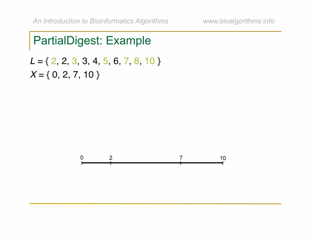
L = { 2, 2, 3, 3, 4, 5, 6, 7, 8, 10 }"X = { 0, 2, 7, 10 }"
PartialDigest: Example

An Introduction to Bioinformatics Algorithms www.bioalgorithms.info
L = { 2, 2, 3, 3, 4, 5, 6, 7, 8, 10 }"X = { 0, 2, 7, 10 }"
• Take 6 from L and make y = 6. • Unfortunately D(y, X) = {6, 4, 1 ,4}, which is not a subset of L.
Therefore we won’t explore this branch.
6
PartialDigest: Example

An Introduction to Bioinformatics Algorithms www.bioalgorithms.info
L = { 2, 2, 3, 3, 4, 5, 6, 7, 8, 10 }"X = { 0, 2, 7, 10 }"
• This time make y = 4. D(y, X) = {4, 2, 3 ,6}, which is a subset of L so we will explore this branch. We remove {4, 2, 3 ,6} from L and add 4 to X.
PartialDigest: Example

An Introduction to Bioinformatics Algorithms www.bioalgorithms.info
L = { 2, 2, 3, 3, 4, 5, 6, 7, 8, 10 }"X = { 0, 2, 4, 7, 10 }"
PartialDigest: Example

An Introduction to Bioinformatics Algorithms www.bioalgorithms.info
L = { 2, 2, 3, 3, 4, 5, 6, 7, 8, 10 }"X = { 0, 2, 4, 7, 10 }"
• L is now empty, so we have a solution, which is X.
PartialDigest: Example
An Introduction to Bioinformatics Algorithms www.bioalgorithms.info
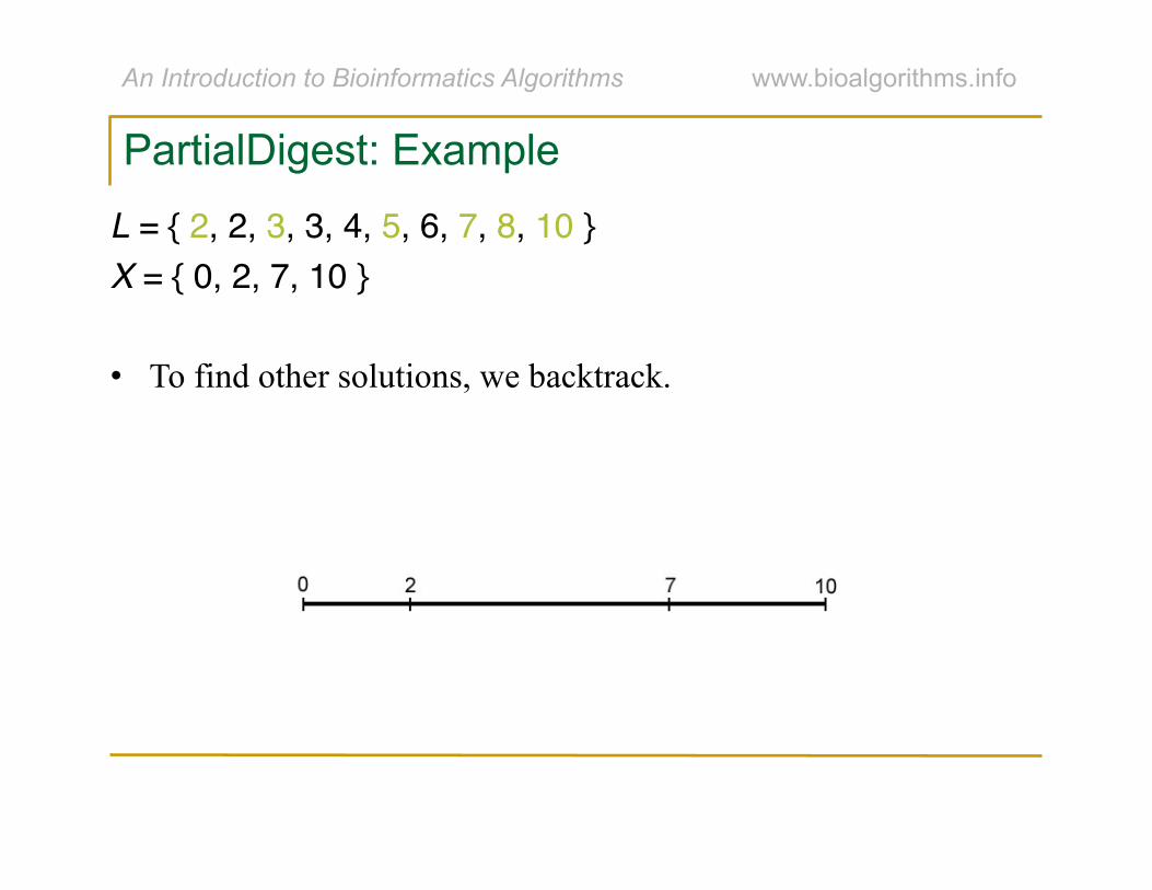
L = { 2, 2, 3, 3, 4, 5, 6, 7, 8, 10 }"X = { 0, 2, 7, 10 }"
• To find other solutions, we backtrack.
PartialDigest: Example

An Introduction to Bioinformatics Algorithms www.bioalgorithms.info
L = { 2, 2, 3, 3, 4, 5, 6, 7, 8, 10 }"X = { 0, 2, 10 }"
• More backtrack.
PartialDigest: Example
An Introduction to Bioinformatics Algorithms www.bioalgorithms.info
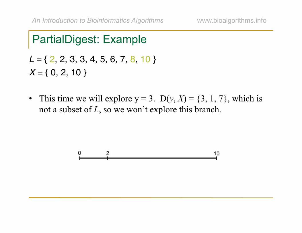
L = { 2, 2, 3, 3, 4, 5, 6, 7, 8, 10 }"X = { 0, 2, 10 }"
• This time we will explore y = 3. D(y, X) = {3, 1, 7}, which is not a subset of L, so we won’t explore this branch.
PartialDigest: Example
An Introduction to Bioinformatics Algorithms www.bioalgorithms.info
L = { 2, 2, 3, 3, 4, 5, 6, 7, 8, 10 }"X = { 0, 10 }"
• We backtracked back to the root. Therefore we have found all the solutions.
PartialDigest: Example
An Introduction to Bioinformatics Algorithms www.bioalgorithms.info
• Still exponential in worst case, but is very fast on average.
• Informally, let T(n) be time PartialDigest takes to place n cuts. • No branching case: T(n) < T(n-1) + O(n)
• Quadratic • Branching case: T(n) < 2T(n-1) + O(n)
• Exponential
Analyzing the PartialDigest Algorithm