dkpartement d’lnformatique, universit6 de montrpal, c. … · dkpartement d’lnformatique,...

JOURNAL OF APPROXIMATION THEORY 4, 147-158 (1971)

Topology of a General Approximation System and Applications

ALEX BACOPOULOS

Dkpartement d’lnformatique, Universit6 de MontrPal, C. P. 6128, MontrPal 101, Canada.

Communicated by G. Meinardus

Received October 2, 1969

DEDICATED TO PROFESSOR LOTHAR COLLATZ ONTHE OCCASION OF HIS SIXTIETH BIRTHDAY

1. INTRODUCTION AND STATEMENT OF THE PROBLEM

In this paper we shall examine a generalization of the classical problem of approximation in normed linear spaces which we will call “vectorial approximation.” Sections 1 and 2 contain a statement of the problem, examples, and some topological considerations used in the general theory. In Sections 3 and 4, the questions of existence, uniqueness and characterization are answered for special types of vectorial approximation.

Let X be a linear space of real-valued functions on [a, b], Yan n-dimensional subspace of X, and let Li be linear operators on X, for i = 1, 2,..., k. We denote by / . Ii an (abstract) norm on Xi = {Li(x), x E X}, i = 1, 2,..., k. A vector-seminorm (11 . 11, <.) is defined as follows:

Ii XII = (I &(x)11 , I L(X)12 ,..., I LdX)ld2 for x E X,

and )/ x1 11 <. /I x2 (), where x1 , x2 E X, if and only if / Li(x,)li < I &(x%)1, for all i = 1, 2,..., k. If at least one Li is the identity operator, (11 . 11, <*) will be called a vector-norm. Given a basis (yJ of Y and an x~X, we will say that a = (A, ) AZ )...) A,) or y, = Cy=, A,y, is a vectorial approximation to x. We define FX(ol) = jj x - ya 11. We call CY or yw a best vectorial approximation to x if F,(a) is a minimal point of the range of F, i.e., if there is no /3 E En such that F%(p) <* F=(a) and P’%(p) # P’%(a).

For notational convenience, we shall use the absolute value symbol 1 * 1 to denote ordinary (real-valued) norms. The symbol /I * jl we will reserve for vector-valued norms and seminorms. If K is a subset of Euclidean n-space P, the symbol F,(K) will represent the set {F,(a) : N E K}. We will denote by M(K) the set of minimal points of F,(K). Where the meaning is clear, we shall write M and F(a) instead of M(E”) and Fz(~). The problem of vectorial

147

148 BACOPOULOS

approximation is, roughly, the study of the equation F(a) = p, for each ZL E M. In way of justification of the terms “vector-norm” and “vector- seminorm” we note the following relations which are easy to verify:

II x + Y II < * II x II + II Y il9

for all X, y E X and all real 19. Furthermore, if at least one Li is the identity operator, then /I x I/ = (0,O ,..., 0) implies x = 0.

2. EXAMPLES AND A GENERAL THEORY OF VECTOR-NORMS

In the following examples [(a)-(e)] of vectorial approximation, let X be (quite arbitrarily) the space C’[O, 11, let Y be the class of polynomials of degree < 5, and let x E X.

(a) Approximation of a function with respect to two norms.

1 * II = Chebychev (sup) norm, j * I2 = L3 norm,

L, = L, = Z (identity).

(b) Approximation of a function and its derivative with respect to the Chebychev (sup) norm.

I * II = sup norm, 1 * I2 = sup norm,

L1 = I, d

L,=-&.

(c) Approximation of a function in L” norm, and its seventh derivative in L3 + sup norm.

j * jl = Lp norm, / . I2 = (L3 norm) + (sup norm),

L1 = z,

TOPOLOGY OF A GENERAL APPROXIMATION SYSTEM 149

(d) Approximation of a function fin the sup norm, off’ in L3 norm, and off in L1.

/ . II = sup norm,

1 . I2 = L3 norm,

/ . I3 = L1 norm,

L, = z,

d L,=p

L, = z.

DEFINITION. Given E 2 0, g(x) is said to E-interpolatef (x) at x1 , x4 ,..., x, iffCL lf(4 - gW < E.

Observe that O-interpolation is the usual interpolation.

(e) Constrained one-sided approximation, weighted E-interpolation and L” approximation. Require that x(t) - ya(t) 2 0 on [O,l]; oh a polynomial of degree < 5.

/ . jl = Lp norm,

/ * I2 = sup norm,

1 * j3 = L1 norm,

L, = z,

L, = CaiEi,

L, = z,

where ai are positive weights, and ei are the point functionals defined by L(f) = f(Xi).

(f) Application to model theory.

A standard electronic filter approximates, in the supremum norm, an ideal input-output characteristic. The number of the so-called lumped parameters (resistors, capacitors, etc.) equals the number of parameters of the approximation, while the way in which the lumped parameters are arranged (in series, in parallel, or in some other combination) corresponds to the type of approximation (linear, rational, etc.). In general, let S be an object we are interested in simulating by models &Z(U), 01 E J (a is a vector of parameters which varies over a set J). Let Li be linear operators acting on the ~&‘(a) and on S and let / . /i (i = 1, 2,..., k) be a gauge of the goodness of fit of the i-th simulation feature. We use a minus sign “-$” formally, to be interpreted in

150 BACOPOULOS

context, and the range of each 1 * Ii is ordered. For example, for some fixed i, let Li be the color operator, let L,(S) = yellow, and let {&(a), 01 E J} = {orange, black, blue, green}. If it is further judged that l(yellow) -i (orange)l, = good, I(yellow) -i (blue)/i = I(yellow) -i (green)li = medium, /(yellow) -i (black)li = bad, we have such an ordering. Briefly, given S, a model space {A(a), OL E J}, linear operators Li on S u {A&‘(X)), interpre- tations of the binary operations -i (i = 1, 2,..., k) which induce meaningful orderings on 1 . Ii , then a best modeI A?(a) is one for which F,(a) is a “best vectorial approximation.” The realizability of a best model is synonymous to M(J) being nonempty.

In what follows we prove some general theorems on vectorial approximation.

THEOREM 2.1. F,(a) is a continuous function of iy.

Proqf. Let cy = (A, , A, ,..., A,), /3 = (B, , Bz ,..., B,). The absolute value of the s-th component of the k-vector F(a) - F(:(p) is

L, and the yi’s are fixed; so F,(a) is a continuous function of a.

COROLLARY. If K is a compact subset of En, M(K) is nonempty.

Proof. F(K) is also a compact subset of E”; so the infima of chains of F(K) relative to the usual, coordinate-wise partial ordering <. of E” are assumed.

THEOREM 2.2. M(E”) = M(Z”), for some cube I” C En.

Proof. Define an extreme minimum to be a point (mls, m2S,..., mks) with the property that inf,,, ( Ls(x - y)l, = mss. Note [l] that in case, for some s, L, is the identity operator, there is a y E Y such that / x - y IS = mss and, hence, the extreme minimum is a point of M.

For every s, 1 < s < k, an extreme minimum (mlS, mzs,..., mBs) does exist. Choose one. Now let p = max{mji : i = 1, 2 ,..., k, j = 1, 2 ,..., k} and define KS = max{i L,(x)l, , CL}. For y E En in the complement of

A = {Y : II Y II <- 3(K,, K, >..., &)h

we have / L,(y)l, > 3K, for some s.


Therefore,

I -&(x - v)l, 2 I &(Y)l, - I -U& 3 3K - I L(x)l > & 3 my m,i.

so, (PI > /&I ,..., pCLB) = P(y) $ M(P). Hence, M(E”) C&4). Now, the closed bounded set A is compact. Therefore, first, the infima of descending chains in F(A) are assumed, and, secondly, there exists I” 1 A such that M(E”) = M(I”). In what follows, we will write A4 instead of M(En).

THEOREM 2.3.

(a) F-Q) is a convex subset of En, for each t_~ E M. (b) M is closed. It consists of one point [f and only if the extreme minima

satsify (mli, mzi ,..., mki) = (m,j, mzj ,..., mki) for all i, j.

Proof of (a). Let F(a) = F(p) = CL; then, for 0 < 8 < 1,

F(Bol + (1 - @/3) <* OF(a) + (I - 0) F(p) = p.

Since TV E M, F(&Y + (1 - Q3) = p. The proof of (b) is straightforward. Also, (b) can be strengthened as

follows:

THEOREM 2.4. Let k = 2 and let 01~ and 01~ be best (ordinary) approximations with respect to I * I1 and I * I2 , respectively. [f F(q) f F(ol,) then M is a Jordan arc.

Proof. See [2], p. 81. The following theorem is a generalization of the classical case k = 1.

Its complexity stems from the fact that, unlike the case k = 1, compact connected sets in Ek are generally hard to characterize. Let I” be such that M(Zn) = M(E,) (see Theorem 2.2). For simplicity of notation we denote by S the compact, connected set F(Z”) C Ek.

THEOREM 2.5. S is compact, locally connected, arcwise connected, and has a trivial k - 1 homotopy group, i.e., IT,_,(S) = 0.

Proof. Local connectivity follows from the Hahn-Mazurkiewicz Theorem. Arcwise connectivity follows from the fact that a Peano space is arcwise connected [7, p. 1161.

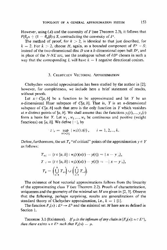
To prove 17,_,(S) = 0, consider the case k = 2. If lir,(S) f 0, there exists a bounded component H of E2 - S. This component contains a disc D because of the compactness of S (see Fig. 1).

Let p be the center of such a disc D. Now move D in the N-NE direction until the N-NE arc of D hits a first point a ES. By the compactness of S,

152 BACOPOULOS

S N-NE

FIGURE 1

such a point exists. We assume, without loss of generality, that it is not the midpoint of the N-NE arc, for otherwise change slightly the preferred N-NE direction. From the point a draw a ray L of slope --I until L hits S at b for the first time. It follows that there exists a neighborhood N(a) in E2 with the property that

where

N(a) n (u O(z)) n S = o, (4 ZEL

L”(z)={x:x~E~,x<.zj,

i.e., the points of L n N(a) are “locally S-W accessible.” Now, by the continuity of F and the convexity of In, there exists a 9,,

,O < 0, < 1, such that

where

F&a + (1 - &,>P) E: N(a) n S,

a E F-l(a), /3 E F-l(b).


However, using (A) and the convexity of F (see Theorem 2.3), it follows that mP + (1 - tm e s> contradicting the convexity of I”.

The method of proof, for k > 2, is identical to that just described, for k = 2. For k > 2, choose H, again, as a bounded component of E” - S; instead of the two-dimensional disc D use a k-dimensional open ball D”, and in place of the N-NE arc, use the analogous subset of aDB chosen in such a way that the corresponding L will have k - 1 negative directional cosines.

3. CHEBYCHEV VECTORIAL APPROXIMATION

Chebychev vectorial approximation has been studied by the author in [Z]; however, for completeness, we include here a brief statement of results, without proofs.

Let x E C[a, b] be a function to be approximated and let Y be an n-dimensional Haar subspace of C[a, b]. That is, Y is an n-dimensional subspace of C[a, b] such that zero is the only function in Y which vanishes at n distinct points of [a, b]. We shall assume that the functions yl(t),..., yn(f) form a basis for Y. Let w1 , w2 ,..., wk be continuous and positive (weight functions) on [a, b]. We define I * Ii by

I z Ii = SUP I w(t> z(t>i, i = 1, 2 ,..,, k. Wa,bl

Define, furthermore, the set T, “of critical” points of the approximation y E Y as follows:

T+i = {t E [a, bl : w&)(x(~> - v(t)) = I x - y Ii}, T-i = {t E [a, b] : Wi(t)(X(t) - y(t)) = -1 X - JJ ii>,

Tv= (;T++‘(@-t). i-1 ,

The existence of best vectorial approximations follows from the linearity of the approximating class Y (see Theorem 2.2). Proofs of characterization, uniqueness and the geometry of the minimal set Mare given in [2, 31. Observe that the following, perhaps surprising, results are generalizations of the standard theory of Chebychev approximation, i.e., k = 1 [l].

The function F,(a) : En --+ E” and the minimal set M here are as defined in Section 1.

THEOREM 3.1 (Existence). Zf p is the injimum of any chain in {F$(oI): 01 E E”}, then there exists o( E En such that FE(~) = p.

154 BACOPOULOS

THEOREM 3.2 (Geometry). Let k = 2 and let 01~ and 01~ be the best (ordinary) approximations with respect to / * jl and I . I2 , respectively. Then the minimal set M is a Jordan arc if and only if 01~ f 01~ . If LYE = 01~ , M is a point.

THEOREM 3.3 (Characterization). Let x E C[a, b] and let y E Y. Then the following statements are equivalent:

(a) y is a best vectorial approximation to x. (b) The origin of Euclt’dean n-space En belongs to the convex hull oj

{o(t)f : t E T,}, where o(t) = - 1 if t E &, TWi , o(t) = + 1 tf t E Uf=, T+i and f = h(t), y&L.., y&N.

(c) There exist n + 1 points t, < tz < .*. < ta+l in T, , satisfying a(tJ = (- l)i+l a(tJ.

THEOREM 3.4 (Uniqueness). Each best vectorial approximation is unique, i.e., given p E M, there is only one (II E En such that Fz(ol) = t.~.

Observe that the uniqueness of Theorem 3.4 does not preclude the existence of several best vectorial approximations. In fact, Theorem 3.2 implies that, in general, there will be a whole Jordan arc of best vectorial approximations. Finally, note that much of this theory holds for more general approximating classes Y [2, 31.

A simple example which illustrates Theorems 3.1-3.4 is the following: Let x(t) = t be approximated by constants {IX}, let k = 2, w1 = 1, and

I S--E --t-t, wz(t) = s

O<ttS,

t, S<t<l.

For small S > 0 and E > 0, it is easy to verify that the best approximations are those oi satisfying Q < 01 < -2 + 2 ~‘2, and that the error of each best approximation exhibits vector-alternation. It is also seen that M here is the line segment joining the points

F(8) = (4, B) and F(-2+2d/z)=(-2+24/2,3-222).

4. L, VECTORIAL APPROXIMATION

Let X = C[a, b] and let (.h and (.)Z be two inner products on X which induce, in the usual fashion, the norms 1 * I1 and / * 12, respectively. Let Y be an n-dimensional subspace of X, spanned by an orthonormal (with respect


to (.)J basis z1 , z2 ,..., z, . Given x E X to be approximated, we define the two-dimensional vector-valued function F(:(ol) = 11 x - ya 11 by

F(a) = (l/(x - y, , x - yJ1 , z/(x - y, ) x - y,),),

where yX = cb, Aizi . The problem here is to determine the minimal set M and, given p E M, to determine all oi’s which satisfy the equation F(a) = CL. Observe that such 01 are generalizations of the classical Fourier coefficients. The equation F(a) = p will be shown to have a unique solution 01. Further- more, using the method of Lagrange multipliers, 01 will be given explicitly in terms of the solution of an algebraic equation in one unknown and of degree 217.

THEOREM 4.1 (Existence). If p is an infimum of the set {F(a) : UI E E”}, then there exists an (II E En satisfying F(a) = CL. Hence M # 0.

Proof. This follows from Theorem 2.2.

THEOREM 4.2 (Geometry). M is either a point or a Jordan arc.

Proof. This is a special case of Theorem 2.4.

THEOREM 4.3 (Solution ofF(a) = p). Let x E C[a, b] and p = (m,, mz) E M. The solution 01 = (A, , A, ,..., A,) is unique and is given by

N’k

where:

A, = - z + (x, zdl, k = 1, 2,. . . , n, e

NI, is the determinant of the n x n matrix {Nij},

Nlc’ is the determinant of the n x n matrix {N&S,

Xi = t Nii i_f’j*i, Mi if j = i,

Nij = bilbj, + bizbj, + .*. + bi,bj, if i *.A

Nii = b;, + bX + **. + bf, + h,

Mm = .f 6, wi>z bmi - i (x, 41 : hnsbis , i=l i=l SC1

and where h, wi and bij will be defined in the proof.

156 BACOPOULOS

Proof (by construction). Let {wi} be the Gram-Schmidt orthonormal sequence relative to (s)~ , where wk = xi=, akizi . Let {bki) be the inverse matrix of {a,J. Using standard Fourier theory on the expression y = x - C Aizi , we have

((Y, Yh 2 (Y, Y)J = XII - i (~3 zd? $ i (Ai - (X2 Zi)d’ i=l i=l

where

’ Cx2 x>i - f Cx, wi>2 + i (4 - Cx, 5 i=l i=l

Bi = f A,b,i. S=l

The remainder of the construction is a standard application of Lagrange multipliers. It involves minimizing ( y, Y)~ as a function of a, where a: satisfies the constraint (y, y), = m12. The resulting n(X) = (A, , A, ,,.., A,) is that given in the statement of Theorem 4.3. h is solved for by substituting the a(h) in the constraint equation. This yields an algebraic equation for h of degree 2n which may be solved by the various standard iterative methods. The details of this construction may be found in [4].

The uniqueness of 01 is seen as follows: From the above constructive proof it is clear that h, and, therefore, 01 can have at most 2n values. By Theorem 2.3, F-l(p) is convex, and the result follows.

As a simple illustration of the above, we will compute M and the o( satisfying F(a) = p E M, where F is given by

F(A,,A2)=~~t2-A2$t-AA,$~~ and

and

Observe that, here, 12 = 2, x = t2 and the orthonormal vectors are

z&=, z2 = - 3 2 t, w1 = - d!- 2 w2 = 2. 37 1.

We evaluate

(t2 z ) = fl > 11 3 ’ (t”, Z2)l = 0, (t”, t2)1 = ;


(P, P), = f 3-f, IA- (P, MQ2 = -7j- ) @“, w2)2 = 0,

rrd\/z 1 ---_ A,=- 2A;( ,$+$, A,=O.

77

Substituting into the constraint equation (A# = m, - (8/45), we get for F(M) the set of all (A, , A,) given by

1/z A, = (T - ml - &)li.’

3 . A, = 0,

Also, the coordinates of A4 are given by

Z/(t”, = (A + (Al - $j2 - A?p)l’*,

d/(r2, = (; + (Al + - $j2 + (A2 +jt)1’2, (A,, A,) EF(M).

5. COMMENTS AND UNSOLVED PROBLEMS

Note that, perhaps surprisingly, much of the classical structure extends to the vectorial context in the cases of the best understood approximation spaces, namely Chebychev and L2. One can, of course, generate a plethora of unsolved problems by specializing the norms and the operators. Two such interesting problems are

1. Characterize all best vectorial approximations with respect to a vector-norm composed of a supnorm and an L2 norm.

2. Characterize all best vectorial approximations with respect to a vector-norm composed of the sup-norm of a function and the sup-norm of its derivative (see related work of P. J. Laurent, Num. Math. 10 (1967)).

ACKNOWLEDGMENTS

The author wishes to thank his thesis advisor Professor Preston Hammer for many stimulating discussions of nonstandard problems in approximation theory, including helpful comments on this paper. We also wish to thank Professors Branko Griinbaum and John G. Hocking for pointing out some difficulties in generalizing Theorem 2.4 to the case k > 2. Answers to some questions originally proposed by Professor Lothar Collate and related to Section 2 may be found in [8].

158 BACOPOULOS

REFERENCES

1. N. I. ACHIEZER, “Theory of Approximation” (English translation), Ungar, New York, 1956.

2. A. BACOPOULOS, Nonlinear Chebychev approximation by vector-norms, J. Approxima- tion Theory 2 (1969), 79-84.

3. A. BACOPOULOS AND G. TAYLOR, Vectorial approximation by restricted rationals, Math. Systems Theory 3 (1969), 232-243.

4. A. BACOPOULOS, “Approximation with Vector-Valued Norms in Linear Spaces,” Doctoral thesis (13, 761), University of Wisconsin, Madison, 1966.

5. G. BIRKHOFF, “Lattice Theory,” revised ed., Amer. Math. Sot. Colloq. Publ. (Vol. XXV), Providence, RI., 1948.

6. J. DIEUDONN~, “Foundations of Modern Analysis,” Academic Press, New York, 1960. 7. J. G. HOCKING AND G. S. YOUNG, “Topology,” Addison-Wesley, Reading, Mass., 1961. 8. E. BREDENDIEK, Simultanapproximationen, Arch. Rational Mech. Anal. 33 (1969),

307-330.

dkpartement d’lnformatique, universit6 de montrpal, c. … · dkpartement d’lnformatique,...

Documents