dj114/spract7.doc · web viewa marketing analyst for a major shoe manufacturer is considering the...
TRANSCRIPT
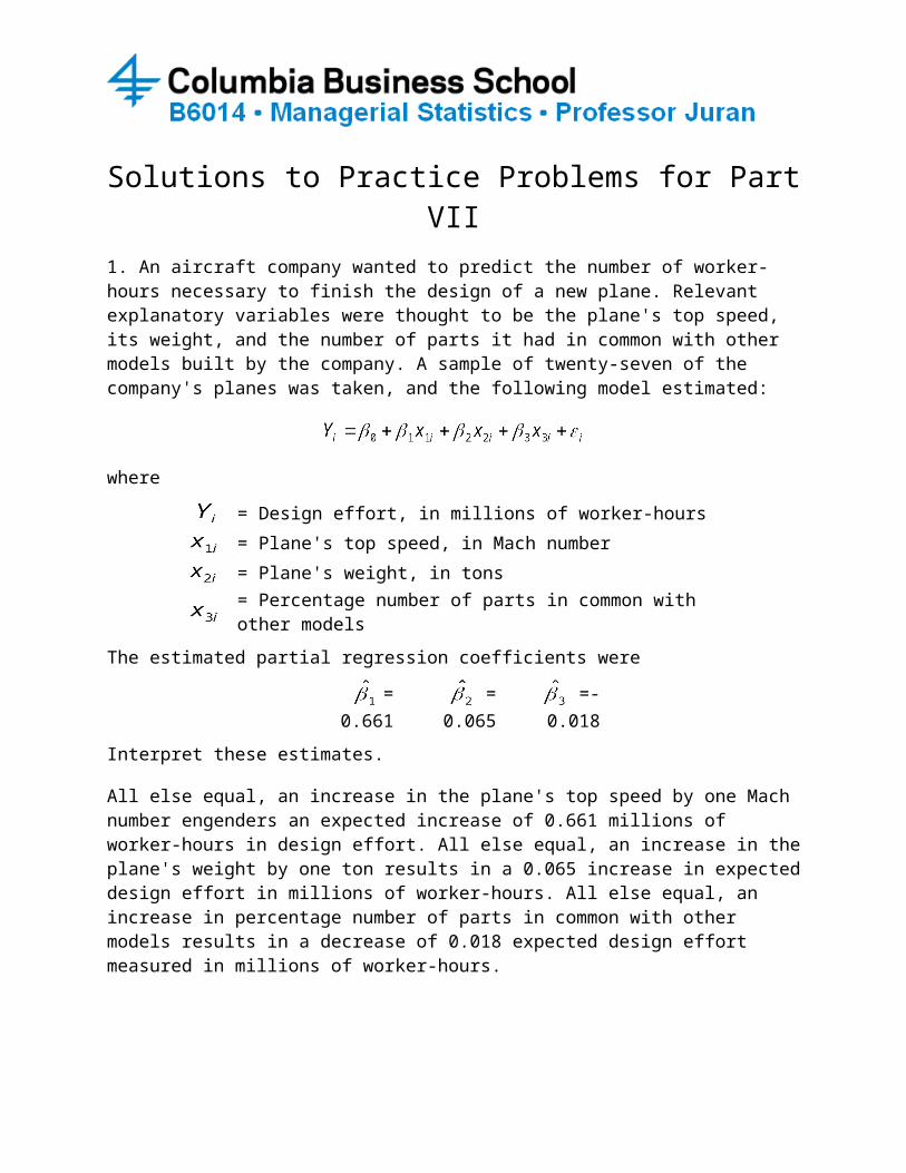
Solutions to Practice Problems for Part VII1. An aircraft company wanted to predict the number of worker-hours necessary to finish the design of a new plane. Relevant explanatory variables were thought to be the plane's top speed, its weight, and the number of parts it had in common with other models built by the company. A sample of twenty-seven of the company's planes was taken, and the following model estimated:
where
= Design effort, in millions of worker-hours= Plane's top speed, in Mach number= Plane's weight, in tons= Percentage number of parts in common with other models
The estimated partial regression coefficients were
= 0.661
= 0.065
=-0.018
Interpret these estimates.
All else equal, an increase in the plane's top speed by one Mach number engenders an expected increase of 0.661 millions of worker-hours in design effort. All else equal, an increase in the plane's weight by one ton results in a 0.065 increase in expected design effort in millions of worker-hours. All else equal, an increase in percentage number of parts in common with other models results in a decrease of 0.018 expected design effort measured in millions of worker-hours.
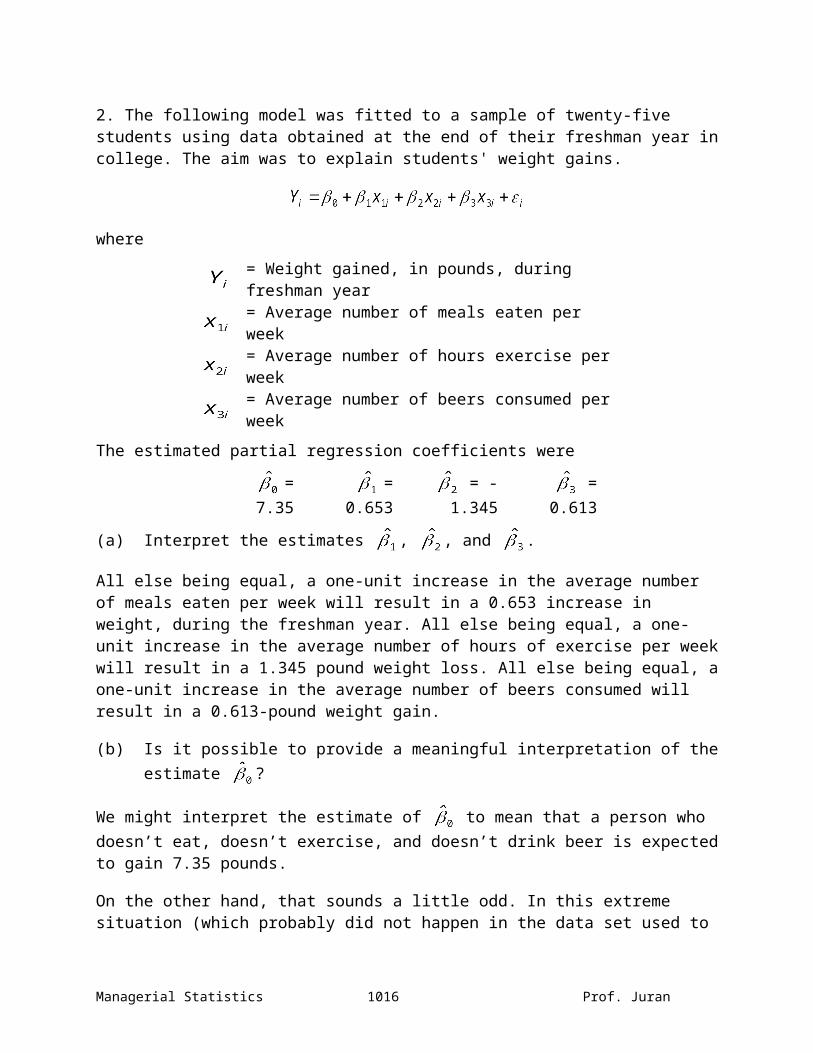
2. The following model was fitted to a sample of twenty-five students using data obtained at the end of their freshman year in college. The aim was to explain students' weight gains.
where
= Weight gained, in pounds, during freshman year= Average number of meals eaten per week= Average number of hours exercise per week= Average number of beers consumed per week
The estimated partial regression coefficients were
= 7.35 = 0.653
= -1.345
= 0.613
(a) Interpret the estimates , , and .
All else being equal, a one-unit increase in the average number of meals eaten per week will result in a 0.653 increase in weight, during the freshman year. All else being equal, a one-unit increase in the average number of hours of exercise per week will result in a 1.345 pound weight loss. All else being equal, a one-unit increase in the average number of beers consumed will result in a 0.613-pound weight gain.
(b) Is it possible to provide a meaningful interpretation of the estimate ?
We might interpret the estimate of to mean that a person who doesn’t eat, doesn’t exercise, and doesn’t drink beer is expected to gain 7.35 pounds.
On the other hand, that sounds a little odd. In this extreme situation (which probably did not happen in the data set used to fit the regression line), we would logically expect a weight loss, not a weight gain.
Managerial Statistics 1016 Prof. Juran
3. In the study of Exercise 1, where the least squares estimates were based on twenty-seven sets of sample observations, the total sum of squares and regression sum of squares were found to be
SST = 3.881 and SSR = 3.549(a) Find and interpret the coefficient of determination.
91% of the variability in design effort can be explained through its linear dependence on the plane's top speed, weight and percentage number of parts in common with other models.
(b) Find the error sum of squares.
SSE = 3.881 - 3.549 = 0.332
(c) Find the corrected coefficient of determination.
(d) Find and interpret the coefficient of multiple correlation.
This is the sample correlation between observed and predicted values of design effort:
Managerial Statistics 1017 Prof. Juran

4. A study was conducted to determine whether certain features could be used to explain variability in the prices of air conditioners. For a sample of nineteen air conditioners, the following regression was estimated:
y = -68.236
+ 0.0023x1
+ 19.729x2
+ 7.653x3
R2 = 0.84
(0.005) (8.992) (3.082)where
y = Price (in dollars)x1 = Rating of air conditioner, in BTU per
hourx2 = Energy efficiency ratiox3 = Number of settings
The figures in parentheses beneath the coefficient estimates are the corresponding estimated standard errors.
(a) Find a 95% confidence interval for the expected increase in price resulting from an additional setting when the values of the rating and the energy efficiency ratio remain fixed.
Note that: n = 19
= 7.653= 3.082
t(15, 0.025)= 2.131
95% C.I.:
Or (1.0853, 14.2207)
Managerial Statistics 1018 Prof. Juran

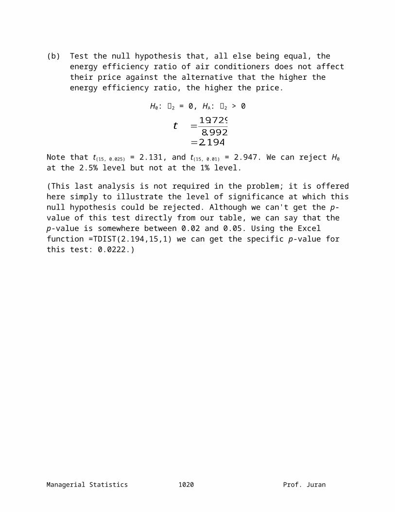
(b) Test the null hypothesis that, all else being equal, the energy efficiency ratio of air conditioners does not affect their price against the alternative that the higher the energy efficiency ratio, the higher the price.
H0: 2 = 0, HA: 2 > 0
Note that t(15, 0.025) = 2.131, and t(15, 0.01) = 2.947. We can reject H0 at the 2.5% level but not at the 1% level.
(This last analysis is not required in the problem; it is offered here simply to illustrate the level of significance at which this null hypothesis could be rejected. Although we can't get the p-value of this test directly from our table, we can say that the p-value is somewhere between 0.02 and 0.05. Using the Excel function =TDIST(2.194,15,1) we can get the specific p-value for this test: 0.0222.)
Managerial Statistics 1019 Prof. Juran
5. In a study of foreign holdings in U.S. banks, the following sample regression was obtained, based on fourteen annual observations:
y = -3.248
+ 0.101x1
- 0.244x2
+ 0.057x3
R2 = 0.93
(0.023) (0.080) (0.00925)
where
y= Year-end share of assets in U.S. bank subsidiaries held by foreigners, as a percentage of total assets
x1
= Annual change, in billions of dollars, in foreign direct investment in the U.S. (excluding finance, insurance, and real estate)
x2 = Bank price-earnings ratiox3 = Index of the exchange value of the dollar
The figures in parentheses beneath the coefficient estimates are the corresponding estimated standard errors.
(a) Find a 90% confidence interval for 1 and interpret your result.Note that: n = 14
= 0.101= 0.023
t(10, 0.05)= 1.812
90% C.I.: = 0.101 1.812(0.023)Or (0.0593, 0.1424)
(b) Test the null hypothesis that 2 is zero, against the alternative that it is negative, and interpret your result.
H0: 2 = 0, HA: 2 < 0
Note that -t(10, 0.01) = -2.764, and -t(10, 0.005) = -3.169.
We can reject H0 at the 1% level but not at the 0.5% level. The p-value for this test (obtained using Excel), is 0.006126.
Managerial Statistics 1020 Prof. Juran

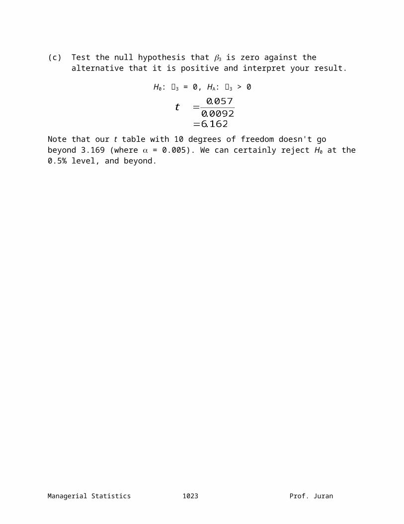
(c) Test the null hypothesis that 3 is zero against the alternative that it is positive and interpret your result.
H0: 3 = 0, HA: 3 > 0
Note that our t table with 10 degrees of freedom doesn't go beyond 3.169 (where = 0.005). We can certainly reject H0 at the 0.5% level, and beyond.
Managerial Statistics 1021 Prof. Juran

6. A survey research group conducts regular studies of households through mail questionnaires and is concerned about the factors influencing the response rate. In an experiment, thirty sets of questionnaires were mailed to potential respondents. The regression model fitted to the resulting data set was
where
= Percentage of responses received= Number of questions asked= Length of questionnaire, in number of words
Part of the SAS computer output from the estimated regression is shown here.
R-Square0.637
Parameter Estimatet For H0:
Parameter = 0Std. Error Of
EstimateIntercept 74.3652
xl -1.8345 -2.89 0.6349x2 -0.0162 -1.78 0.0091
(a) Interpret the estimated partial regression coefficients.
All else being equal, an increase of one question to the questionnaire results in a decrease of 1.834 in expected percentage of responses received. All else being equal, an increase in one word in length of the questionnaire results in a decrease of 0.016 in expected percentage of responses received.
(b) Interpret the coefficient of determination.
63.7% of the variability in percentage responses received is explained by its linear relationship with the number of questions asked and the number of words.
Managerial Statistics 1022 Prof. Juran
(c) Test at the 1% significance level the null hypothesis that taken together, the two independent variables do not linearly influence the response rate.
H0: 1 = 2 = 0, HA: At least one i 0 (i = 1, 2)
OK, no fair. This one requires an alternative formula for the F statistic, which doesn't appear in Levine, but is on the Regression Formula sheet:
Now we look at the 0.01 F table (page E-10 in Levine), and see that the F(2,27,0.01) = 5.49.
Since our observed F is greater than this critical value, we can reject H0 at the 1% level.
(d) Find and interpret a 99% confidence interval for 1.
Note that t(27, 0.005) = 2.771
99% C.I.: = -1.8345 + 2.771(0.6349)Or (-3.5938, -0.0752)
(e) Test the null hypothesis
H0: 2 = 0
against the alternative
HA. 2 < 0
and interpret your findings.
H0: 2 = 0, HA: 2 < 0
Note that -t(27, 0.05) = -1.703, and -t(27, 0.025) = -2.052.
We can reject H0 at the 5% level but not at the 2.5% level.
Managerial Statistics 1023 Prof. Juran

7. Based on data on 2,679 college basketball players, the following model was fitted:
, where:
Y = Minutes played in season
x1 = Field goal percentagex2 = Free throw percentagex3 = Rebounds per minutex4 = Points per minutex5 = Fouls per minutex6 = Steals per minutex7
= Blocked shots per minute
x8 = Turnovers per minutex9 = Assists per minute
The least squares parameter estimates (with standard errors in parentheses):
= 358.848
(44.695)
= -3923.5
(120.6)
= 0.6742 (0.0639)
= 480.04
(224.9)
= 0.2855 (0.0388)
= 1350.3
(212.3)
= 303.81 (77.73) = -891.67
(180.87)
= 504.95 (43.26) = 722.95
(110.98)
The coefficient of determination was R2 = 0.5239
(a) Find and interpret a 90% confidence interval for .
Note that our model is based on a sufficiently large data set to use z as an approximation of t. Specifically,
t(2669, 0.05) 1.645
90% CI: = 480.04 1.645(224.9)Or (110.08, 850.00)
We are 90% confident that playing time will increase by somewhere between 110.08 and 850 minutes per season for every increase of 1 steal per minute.
Managerial Statistics 1024 Prof. Juran

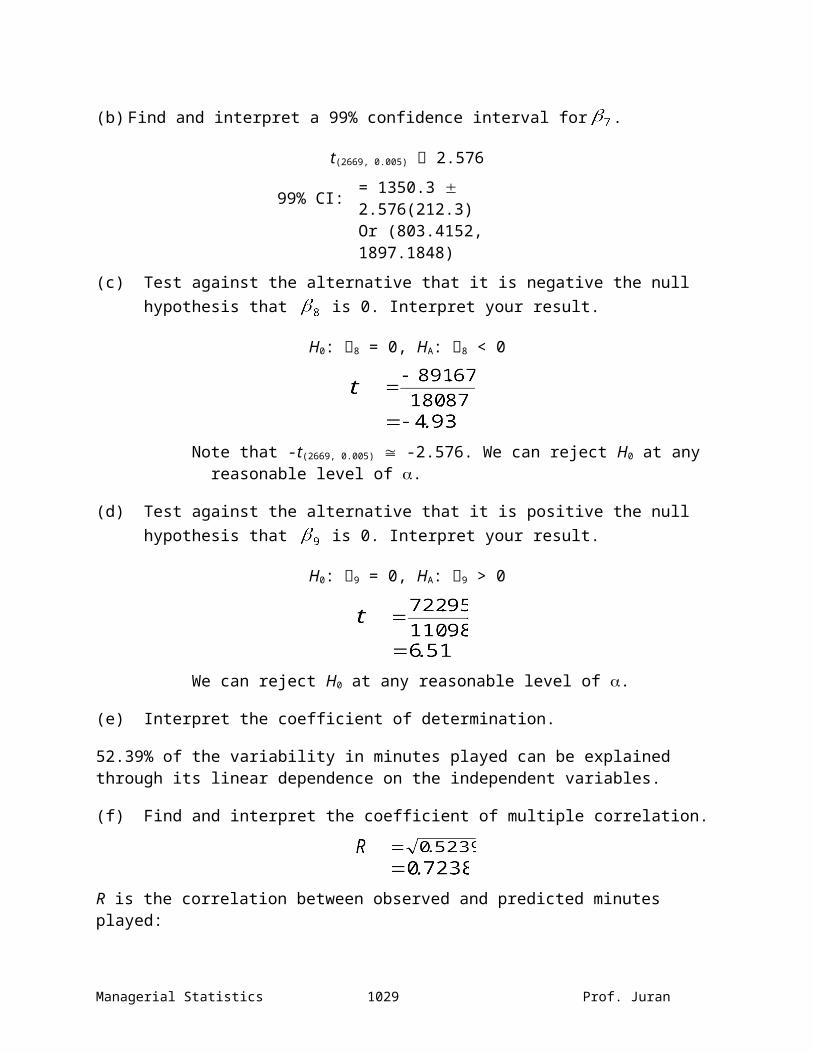
(b) Find and interpret a 99% confidence interval for .
t(2669, 0.005) 2.576
99% CI: = 1350.3 2.576(212.3)Or (803.4152, 1897.1848)
(c)Test against the alternative that it is negative the null hypothesis that is 0. Interpret your result.
H0: 8 = 0, HA: 8 < 0
Note that -t(2669, 0.005) -2.576. We can reject H0 at any reasonable level of .
(d) Test against the alternative that it is positive the null hypothesis that is 0. Interpret your result.
H0: 9 = 0, HA: 9 > 0
We can reject H0 at any reasonable level of .
(e) Interpret the coefficient of determination.
52.39% of the variability in minutes played can be explained through its linear dependence on the independent variables.
(f) Find and interpret the coefficient of multiple correlation.
R is the correlation between observed and predicted minutes played:
Managerial Statistics 1025 Prof. Juran

8. A marketing analyst for a major shoe manufacturer is considering the development of a new brand of running shoes. The marketing analyst wishes to determine which variables can be used in predicting durability (or the effect of long-term impact). Two independent variables are to be considered, X1 (FOREIMP), a measurement of the forefoot shock-absorbing capability, and X2 (MIDSOLE), a measurement of the change in impact properties over time, along with the dependent variable Y (LTIMP), which is a measure of the long-term ability to absorb shock after a repeated impact test. A random sample of 15 types of currently manufactured running shoes was selected for testing. Using Microsoft Excel, we provide the following (partial) output:
ANOVA DF SS MS F SIGNIFICANCE FRegression 2 12.61020 6.30510 97.69 0.0001Residual 12 0.77453 0.06454Total 14 13.38473
VARIABLE COEFFICIENTS STANDARD ERROR t STAT p-VALUEIntercept -0.02686 .06905 -0.39Foreimp 0.79116 .06295 12.57 0.0000Midsole 0.60484 .07174 8.43 0.0000
(a) Assuming that each independent variable is linearly related to long-term impact, state the multiple regression equation.
(b) Interpret the meaning of the slopes in this problem.
For every one-unit increase in FOREIMP, we expect to see a 0.79116-unit increase in LTIMP. For every one-unit increase in MIDSOLE, we expect to see a 0.60484-unit increase in LTIMP.
Managerial Statistics 1026 Prof. Juran

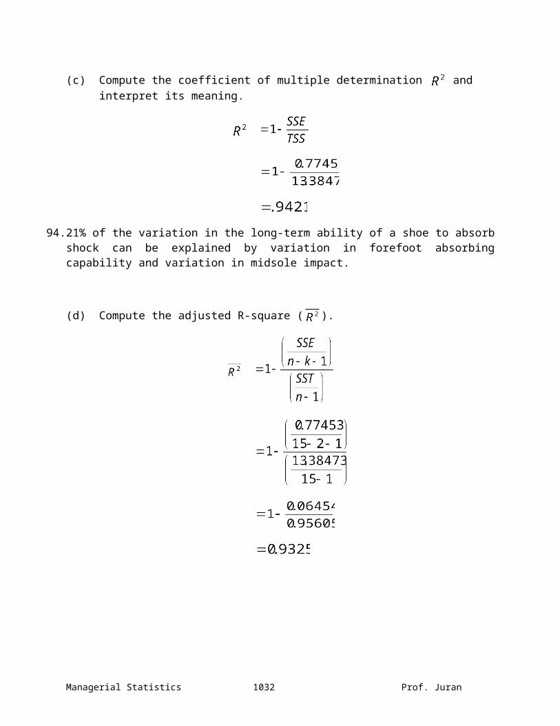
(c) Compute the coefficient of multiple determination and interpret its meaning.
94.21% of the variation in the long-term ability of a shoe to absorb shock can be explained by variation in forefoot absorbing capability and variation in midsole impact.
(d) Compute the adjusted R-square ( ).
Managerial Statistics 1027 Prof. Juran

9. Suppose a large consumer products company wants to measure the effectiveness of different types of advertising media in the promotion of its products. Specifically, two types of advertising media are to be considered: radio and television advertising and newspaper advertising (including the cost of discount coupons). A sample of 22 cities with approximately equal populations is selected for study during a test period of 1 month. Each is allocated a specific expenditure level for both radio and television advertising and newspaper advertising. The sales of the product (in thousands of dollars) and also the levels of media expenditure during the test month are recorded with the following results:
City SALES ($000)RADIO AND TELEVISION
ADVERTISING ($000)NEWSPAPER
ADVERTISING ($000)1 973 0 402 1,119 0 403 875 25 254 625 25 255 910 30 306 971 30 307 931 35 358 1,177 35 359 882 40 25
10 982 40 2511 1,628 45 4512 1,577 45 4513 1,044 50 014 914 50 015 1,329 55 2516 1,330 55 2517 1,405 60 3018 1,436 60 3019 1,521 65 3520 1,741 65 3521 1,866 70 4022 1,717 70 40
Managerial Statistics 1028 Prof. Juran
Excel output:
Regression StatisticsMultiple R 0.8993R Square 0.8087Adjusted R Square 0.7886Standard Error 158.9041Observations 22
df SS MS F Significance FRegression 2 2028032.689
61014016.344
840.158
20.0000
Residual 19 479759.9014 25250.5211Total 21 2507792.590
9
Coefficients Standard Error
t Stat P-value
Intercept 156.4304 126.7579 1.2341 0.2322RADIO&TV 13.0807 1.7594 7.4349 0.0000NEWSPAPER 16.7953 2.9634 5.6676 0.0000
On the basis of the results obtained:
(a) State the multiple regression equation.
(b) Interpret the meaning of the slopes in this problem.
For every one-unit increase in Radio/TV advertising, we expect to see a 13.08-unit increase in Sales.
For every one-unit increase in Newspaper advertising, we expect to see a 16.80-unit increase in Sales.
(c) Predict the average sales for a city in which radio and television advertising is $20,000 and newspaper advertising is $20,000.
(or $753,950.00)
Managerial Statistics 1029 Prof. Juran

(d) Compute the coefficient of multiple determination and interpret its meaning.
80.87% of the variation in Sales is explained by variation in Radio/TV advertising and Newspaper advertising.
(e) Compute the .
Managerial Statistics 1030 Prof. Juran

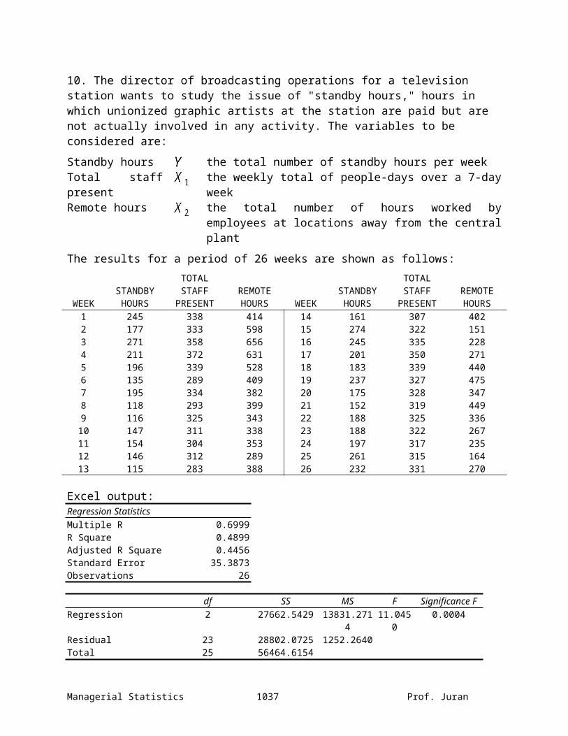
10. The director of broadcasting operations for a television station wants to study the issue of "standby hours," hours in which unionized graphic artists at the station are paid but are not actually involved in any activity. The variables to be considered are:
Standby hours the total number of standby hours per weekTotal staff present
the weekly total of people-days over a 7-day week
Remote hours the total number of hours worked by employees at locations away from the central plant
The results for a period of 26 weeks are shown as follows:
WEEKSTANDBY HOURS
TOTAL STAFF
PRESENTREMOTE HOURS WEEK
STANDBY HOURS
TOTAL STAFF
PRESENTREMOTE HOURS
1 245 338 414 14 161 307 4022 177 333 598 15 274 322 1513 271 358 656 16 245 335 2284 211 372 631 17 201 350 2715 196 339 528 18 183 339 4406 135 289 409 19 237 327 4757 195 334 382 20 175 328 3478 118 293 399 21 152 319 4499 116 325 343 22 188 325 33610 147 311 338 23 188 322 26711 154 304 353 24 197 317 23512 146 312 289 25 261 315 16413 115 283 388 26 232 331 270
Excel output:Regression StatisticsMultiple R 0.6999R Square 0.4899Adjusted R Square 0.4456Standard Error 35.3873Observations 26
df SS MS F Significance FRegression 2 27662.5429 13831.271
411.045
00.0004
Residual 23 28802.0725 1252.2640Total 25 56464.6154
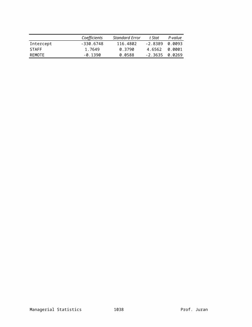
Coefficients Standard Error
t Stat P-value
Intercept -330.6748 116.4802 -2.8389 0.0093STAFF 1.7649 0.3790 4.6562 0.0001REMOTE -0.1390 0.0588 -2.3635 0.0269
Managerial Statistics 1031 Prof. Juran
On the basis of the results obtained:
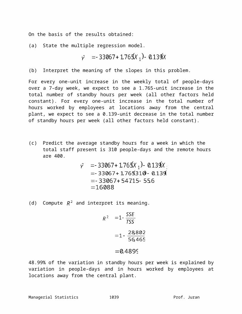
(a) State the multiple regression model.
(b) Interpret the meaning of the slopes in this problem.
For every one-unit increase in the weekly total of people-days over a 7-day week, we expect to see a 1.765-unit increase in the total number of standby hours per week (all other factors held constant). For every one-unit increase in the total number of hours worked by employees at locations away from the central plant, we expect to see a 0.139-unit decrease in the total number of standby hours per week (all other factors held constant).
(c) Predict the average standby hours for a week in which the total staff present is 310 people-days and the remote hours are 400.
(d) Compute and interpret its meaning.
48.99% of the variation in standby hours per week is explained by variation in people-days and in hours worked by employees at locations away from the central plant.
Managerial Statistics 1032 Prof. Juran

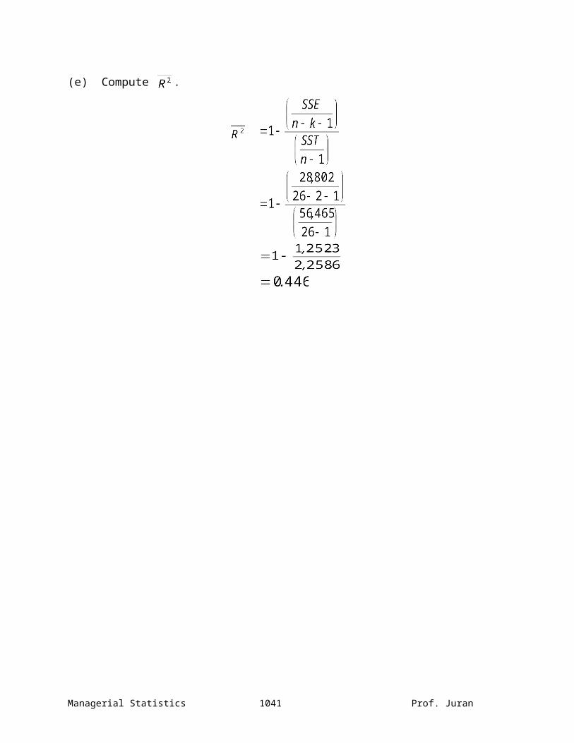
(e) Compute .
Managerial Statistics 1033 Prof. Juran

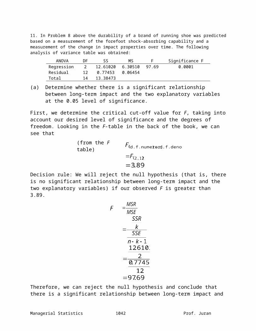
11. In Problem 8 above the durability of a brand of running shoe was predicted based on a measurement of the forefoot shock-absorbing capability and a measurement of the change in impact properties over time. The following analysis of variance table was obtained:
ANOVA DF SS MS F Significance FRegression 2 12.61020 6.30510 97.69 0.0001Residual 12 0.77453 0.06454Total 14 13.38473
(a) Determine whether there is a significant relationship between long-term impact and the two explanatory variables at the 0.05 level of significance.
First, we determine the critical cut-off value for F, taking into account our desired level of significance and the degrees of freedom. Looking in the F-table in the back of the book, we can see that
(from the F table)
Decision rule: We will reject the null hypothesis (that is, there is no significant relationship between long-term impact and the two explanatory variables) if our observed F is greater than 3.89.
Therefore, we can reject the null hypothesis and conclude that there is a significant relationship between long-term impact and the two explanatory variables at the 0.05 level of significance. (This whole procedure is done for you in the Excel output; all you need to do is look at the p-value associated with the F statistic.)
Managerial Statistics 1034 Prof. Juran

(b) Interpret the meaning of the p-value.
The p-value for the F statistic (called Significance F in Excel output) is the smallest value of alpha at which we could reject the null hypothesis in the F test. In this case, the p-value of 0.0001 is sufficiently small to allow us to reject the null hypothesis at any reasonable level of alpha.
Managerial Statistics 1035 Prof. Juran

12. In Problem 9 above the amount of radio and television advertising and newspaper advertising was used to predict sales. Using the computer output you obtained to solve that problem,
(a) Determine whether there is a significant relationship between sales and the two explanatory variables (radio and television advertising and newspaper advertising) at the 0.05 level of significance.
Here is the ANOVA table from our previous regression analysis:
df SS MS F Significance FRegression 2 2028032.689
61014016.344
840.158
20.0000
Residual 19 479759.9014 25250.5211Total 21 2507792.590
9Looking in the F-table in the back of the book, we can see that
(from the F table)
Decision rule: We will reject the null hypothesis (that is, there is no significant relationship between long-term impact and the two explanatory variables) if our observed F is greater than 3.522.
Therefore, we can reject the null hypothesis and conclude that there is a significant relationship between long-term impact and the two explanatory variables at the 0.05 level of significance. (This whole procedure is done for you in the Excel output; all you need to do is look at the p-value associated with the F statistic.)
Managerial Statistics 1036 Prof. Juran
(b) Interpret the meaning of the p-value.
The p-value for the F statistic is the smallest value of alpha at which we could reject the null hypothesis in the F test. In this case, the p-value of approximately 0.0000 is sufficiently small to allow us to reject the null hypothesis at any reasonable level of alpha.
Managerial Statistics 1037 Prof. Juran
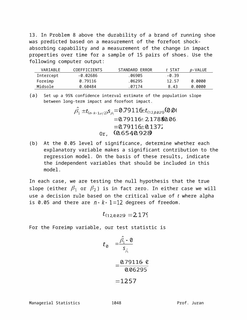
13. In Problem 8 above the durability of a brand of running shoe was predicted based on a measurement of the forefoot shock-absorbing capability and a measurement of the change in impact properties over time for a sample of 15 pairs of shoes. Use the following computer output:
VARIABLE COEFFICIENTS STANDARD ERROR t STAT p-VALUEIntercept -0.02686 .06905 -0.39Foreimp 0.79116 .06295 12.57 0.0000Midsole 0.60484 .07174 8.43 0.0000
(a) Set up a 95% confidence interval estimate of the population slope between long-term impact and forefoot impact.
Or,(b) At the 0.05 level of significance, determine whether each explanatory
variable makes a significant contribution to the regression model. On the basis of these results, indicate the independent variables that should be included in this model.
In each case, we are testing the null hypothesis that the true slope (either or ) is in fact zero. In either case we will use a decision rule based on the critical value of t where alpha is 0.05 and there are degrees of freedom.
For the Foreimp variable, our test statistic is
Therefore, we reject the null hypothesis and conclude that there is a relationship between durability and forefoot shock-absorbing capability. This is also evidenced by the very small p-value in the output associated with the forefoot shock-absorbing capability independent variable (approximately 0.0000).
Managerial Statistics 1038 Prof. Juran
For the Midsole variable, our test statistic is
Therefore, we reject the null hypothesis and conclude that there is a relationship between durability and the change in impact properties over time.
This is also confirmed by the very small p-value associated with the "change in impact properties over time" independent variable (approximately 0.0000).
We conclude that both of these independent variables are useful, and ought to remain in the model.
(Note that these hypothesis tests are done for you in the Excel output; all you need to do is look at the p-value associated with each estimated slope coefficient.)
Managerial Statistics 1039 Prof. Juran

14. In Problem 9 above the amount of radio and television advertising and newspaper advertising was used to predict sales. Use the computer output you obtained to solve that problem.Here is a subset of the Excel output produced before:
Coefficients Standard Error
t Stat P-value
Intercept 156.4304 126.7579 1.2341 0.2322RADIO&TV 13.0807 1.7594 7.4349 0.0000NEWSPAPER 16.7953 2.9634 5.6676 0.0000(a) Set up a 95% confidence interval estimate of the population slope between sales and radio and television
advertising.
Or,(b) At the 0.05 level of significance, determine whether each explanatory
variable makes a significant contribution to the regression model. On the basis of these results, indicate the independent variables that should be included in this model.
In each case, we are testing the null hypothesis that the true slope (either or ) is in fact zero. In either case we will use a decision rule based on the critical value of t where alpha is 0.05 and there are degrees of freedom.
For the Radio & TV variable, our test statistic is
Therefore, we reject the null hypothesis and conclude that there is a relationship between Radio and TV advertising and Sales.
This is also evidenced by the very small p-value in the Excel output associated with the Radio & TV independent variable (approximately 0.0000).
Managerial Statistics 1040 Prof. Juran
For the Newspaper variable, our test statistic is
Therefore, we reject the null hypothesis and conclude that there is a relationship between Newspaper advertising and Sales.
This is also evidenced by the very small p-value associated with the "Newspaper" independent variable (approximately 0.0000).
We conclude that both of these independent variables are useful, and ought to remain in the model.
(Note that these hypothesis tests are done for you in the Excel output; all you need to do is look at the p-value associated with each estimated slope coefficient.)
Managerial Statistics 1041 Prof. Juran
15. A real estate association in a suburban community would like to study the relationship between the size of a single-family house (as measured by the number of rooms) and the selling price of the house. The study is to be carried out in two different neighborhoods, one on the east side of the community and the other on the west side. A random sample of 20 houses was selected with the following results:
SELLING PRICE
NUMBER OF ROOMS NEIGHBORHOOD
SELLING PRICE
NUMBER OF ROOMS NEIGHBORHOOD
109.6 7 East 108.5 6 West107.4 8 East 181.3 13 West140.3 9 East 137.4 10 West146.5 12 East 146.2 10 West98.2 6 East 142.4 9 West
137.8 9 East 123.7 8 West124.1 10 East 129.6 8 West113.2 8 East 143.6 9 West127.8 9 East 160.7 11 West125.3 8 East 148.3 9 West
Excel output:Regression StatisticsMultiple R 0.9311R Square 0.8670Adjusted R Square 0.8513Standard Error 7.7393Observations 20
df SS MS F Significance FRegression 2 6635.4808 3317.740
455.390
80.0000
Residual 17 1018.2487 59.8970Total 19 7653.7295
Coefficients Standard Error
t Stat P-value
Intercept 56.4339 9.8833 5.7100 0.0000ROOMS 9.2189 1.0296 8.9537 0.0000EAST -12.6967 3.5354 -3.5913 0.0023
Using Microsoft Excel:(a) State the multiple regression equation.
Managerial Statistics 1042 Prof. Juran

(b) Interpret the meaning of the slopes in this problem.
For every one-unit increase in the number of Rooms, we expect to see a 9.2189-unit increase in Selling Price (an expected increase of $9,218.90 for each additional room). For every one-unit increase in East, we expect to see a 12.6967-unit decrease in Selling Price (all else being equal, a house on the East side is expected to sell for $12,696.70 less than a house on the West side).
(c) Predict the average selling price for a house with nine rooms that is located on the east side of the community.
(or $126,707.30)
(d) Perform a residual analysis on your results and determine the adequacy of the fit of the model.
A scatter diagram of the residuals doesn’t reveal any obvious pattern:
Managerial Statistics 1043 Prof. Juran
A histogram of the errors seems reasonably bell-shaped, given that we only have 20 data:
Without doing any sophisticated hypothesis tests, it seems reasonable to use the model on the assumption that there is no problem with heteroscedasticity or non-normality of the residuals.
Managerial Statistics 1044 Prof. Juran

(e) Determine whether there is a significant relationship between selling price and the two explanatory variables (rooms and neighborhood) at the 0.05 level of significance.
First, we determine the critical cut-off value for F, taking into account our desired level of significance and the degrees of freedom. Looking in the F-table in the back of the book, we can see that
(from the F table)
You can also get the critical value of F using the Excel function:
=FINV(0.05, 2, 17).
Therefore, we will reject the null hypothesis (that there is no significant relationship between long-term impact and the two explanatory variables) if our observed F is greater than 3.592.
Therefore, we can reject the null hypothesis and conclude that there is a significant relationship between long-term impact and the two explanatory variables at the 0.05 level of significance.
Managerial Statistics 1045 Prof. Juran

(f) At the 0.05 level of significance, determine whether each explanatory variable makes a contribution to the regression model. On the basis of these results, indicate the regression model that should be used in this problem.
In each case, we are testing the null hypothesis that the true slope (either or ) is in fact zero. In either case we will use a decision rule based on the critical value of t where alpha is 0.05 and there are degrees of freedom.
For the Rooms variable, our test statistic is
Therefore, we reject the null hypothesis and conclude that there is a relationship between the number of Rooms and Selling Price.
This is also evidenced by the very small p-value in the Excel output associated with the Rooms independent variable (approximately 0.0000).
For the East variable, our test statistic is
Therefore, we reject the null hypothesis and conclude that there is a relationship between Neighborhood and Selling Price.
This is also evidenced by the very small p-value associated with the "East" independent variable (approximately 0.0023).
We conclude that both of these independent variables are useful, and ought to remain in the model.
Managerial Statistics 1046 Prof. Juran

(g) Set up 95% confidence interval estimates of the population slope for the relationship between selling price and number of rooms and between selling price and neighborhood.
For Rooms:
Or,For Neighborhood:
Or,(h) Interpret the meaning of the coefficient of multiple determination, .
86.7% of the variation in selling prices is explained by the combined effects of the number of rooms and the neighborhood.
Managerial Statistics 1047 Prof. Juran
(i) Compute .
(k) What assumption about the slope of selling price with number of rooms must be made in this problem?
We are implicitly assuming that the effect of the number of rooms on selling price is the same, regardless of which part of town a house happens to be in. We could avoid making this assumption by having a separate model for each of the two sides of town.
Managerial Statistics 1048 Prof. Juran