dividends: from refracting to ratcheting

DIVIDENDS: FROM REFRACTING TO RATCHETING

HANSJORG ALBRECHER†, NICOLE BAUERLE∗, AND MARTIN BLADT4

Abstract. In this paper we consider an alternative dividend payment strategy in risktheory, where the dividend rate can never decrease. This addresses a concern thathas often been raised in connection with the practical relevance of optimal classicaldividend payment strategies of barrier and threshold type. We study the case whereonce during the lifetime of the risk process the dividend rate can be increased andderive corresponding formulae for the resulting expected discounted dividend paymentsuntil ruin. We first consider a general spectrally-negative Levy risk model, and thenrefine the analysis for a diffusion approximation and a compound Poisson risk model.It is shown that for the diffusion approximation the optimal barrier for the ratchetingstrategy is characterized by an unexpected relation to the case of refracted dividendpayments. Finally, numerical illustrations for the diffusion case indicate that with sucha simple ratcheting dividend strategy the expected value of discounted dividends canalready get quite close to the respective value of the refracted dividend strategy, thelatter being known to be optimal among all admissible dividend strategies.

1. Introduction

Starting with de Finetti’s work [12], the study of optimal dividend payout strategiesin collective risk theory has been a very active field of research over the last 60 years.It is nowadays well-known that in order to maximize the expected aggregate discounteddividends until ruin, it is optimal to pay dividends according to a band strategy, which ina number of cases collapses to a barrier strategy, see e.g. [14], [25], [24] and [9]. When thisoptimal control problem is considered with an upper bound on the dividend rate, thenin many cases a refracting dividend strategy (or, synonymously, a threshold strategy) isoptimal (i.e., no dividend payments up to a certain barrier level, and dividend paymentsat maximal allowed rate above that barrier), see for instance [19], [5] for diffusions and[15] and [22] for the compound Poisson process. Since then numerous extensions andvariations of the dividend problem have been considered, many of which leading to intri-cate and interesting mathematical problems, see e.g. [3] and [7] for surveys on the topic.Among these variations, some also address the issue that the theoretically optimal re-fraction strategy may not be realistic when it comes to implementation in practice. Oneconstraint is that dividends can only be paid out in a discrete rather than a continuous-time fashion, see [1] for a contribution in this direction for random discrete payment times.Another problem with the threshold strategy is the strong variability of payment patternsacross time. In [8] it was proposed for a diffusion process to consider dividend paymentsthat are proportional to the current surplus level, which leads to much smoother dividendstreams. Recently, the respective analysis of performance measures was extended to thecompound Poisson model in [2]. In [10] and [11] the aim was to maximize risk-sensitivedividend payments in discrete time which, in case of exponential utility, results in opti-mizing a weighted criterion of expectation and variance of the dividends.

In this paper we would like to consider another constraint that is often mentioned indiscussions with practitioners. Concretely, it is at times considered desirable to have adividend payment stream that does not decrease over time (which we will refer to as

1

2 H. ALBRECHER, N. BAUERLE, AND M. BLADT

a ratcheting strategy, see e.g. [13]). One reason is that a decrease may have a negativepsychological impact on shareholders and the considered value of the company in general.Sticking to the analytically much more tractable situation of a continuous-time model,the over-all mathematical question could then be to find the optimal dividend paymentpattern with a non-decreasing dividend rate. This general optimal control problem isa considerable challenge, as one immediately is put into a two-dimensional setting withone variable keeping track of the current dividend rate, so that the usually advantageousMarkovian structure of the surplus process is lost even for simple processes. We hencein this paper will consider only a first step towards improving the understanding of thisgeneral problem, namely to allow for a constant dividend rate through-out the lifetime ofthe risk process, which once during the lifetime can be increased to a higher level. Thetask then is to find the optimal rates before and after that change, and the surplus levelat which this change should take place, so that the expected over-all discounted dividendpayments are maximized. The only constraint in this context will be that the dividendrate must never exceed the drift rate of the original process. This setting leads to quiteexplicit results and will give some insight into the nature of the problem. A particularfocus will be given on the comparison of the resulting optimal ratcheting strategy withthe best refracting strategy, which is known to be optimal among all admissible dividendstrategies in the absence of such a ratcheting constraint.

We will first deal with the general case of spectrally-negative Levy processes in Section2. After collecting some necessary preliminaries, we adapt an existing formula for refrac-tion strategies that also allows for dividend payments below the barrier. We then derivea general formula for the expected discounted dividend payments until ruin accordingto a ratcheting strategy in terms of the scale function of the underlying Levy process,and derive a criterion for the optimal ratcheting barrier. Subsequently, in Section 3 werefine the analysis for the case of a pure Brownian motion with drift (diffusion approx-imation). While many of the respective formulas can in fact be obtained from Section2 by substituting the simple form of the respective scale function, we derive a numberof formulas in that section in a self-contained, sometimes more direct, way. This addsanother perspective to the problems under study, and also allows to read parts of thatsection independently of the general Levy fluctuation theory that underlies the approachin Section 2. We then give some numerical illustrations on the performance of both therefracting and ratcheting strategy, which somewhat surprisingly indicate that the bestratcheting procedure is not far behind the best refracting (and hence over-all best) divi-dend strategy. We also derive a somewhat surprising criterion for the optimal ratchetingbarrier in terms of a matching with a refracting strategy. In Section 4 we then proceedto work out the formulas of Section 2 to the particular case of a Cramer-Lundberg riskmodel with hyper-exponential claim sizes. We also show that the optimality criterion forthe diffusion case mentioned above no longer holds in the compound Poisson setting, thereason being the non-differentiability of the refraction value function at the barrier level.One natural concern for the implementation of a ratcheting strategy of the above kind isthat after the switching, the higher dividend rate will always stay, even when the surpluslevel gets low. Correspondingly one may expect that ruin is more likely or happens ear-lier, particularly when the optimal barrier level is chosen according to the profitabilitycriterion of maximal expected dividend payments. Also, the optimal racheting barrieris in general higher than the optimal refraction barrier. In Section 5 we discuss thisissue further and quantify it in terms of expected ruin time, given that ruin occurs. Thenumerical results in fact indicate that, conditional on ruin to occur in finite time, the

DIVIDENDS: FROM REFRACTING TO RATCHETING 3

expected time to ruin is larger for the ratcheting strategy. Finally, Section 6 containssome conclusions.

2. The Spectrally-Negative Levy Risk Model

Let us consider a spectrally-negative Levy process Y = {Yt}t≥0, i.e. a Levy processwith only negative jumps, and which is not a.s. a non-increasing process. We assumethat Y0 = x ≥ 0 and the drift of this process is positive, and call such a Y a Levy riskprocess. Our focus in this paper will be on risk processes constantly paying out dividendsat rate c1 ≥ 0 (so possibly c1 = 0), and in certain periods (to be specified) at an increasedrate c1 + c2, with c2 > 0. Correspondingly, the Levy processes of interest are

Xt = Yt − c1t, Xt = Yt − (c1 + c2)t.

for all t ≥ 0. Define the Laplace exponent

ψ(θ) := logEeθX1 ,

which is finite for at least all θ ≥ 0, and denote by Φ(δ) the largest root of the equationψ(θ) = δ. The δ-scale functions W (x) and Z(x) of the process X are defined for anyδ ≥ 0 as ∫ ∞

0

e−uxW (x) dx =1

ψ(u)− δ, u > Φ(δ),

Z(x) = 1 + δ

∫ x

0

W (y)dy.

The respective δ-scale functions for the process X will be denoted by W(x) and Z(x),respectively, and φ(δ) shall be the corresponding largest root of ψ(θ)− c2θ = δ.Define now for a fixed b ≥ 0 the first passage times

τ−0 := inf{t ≥ 0 : Xt < 0}, τ+b := inf{t ≥ 0 : Xt > b}.

We will be working on a canonical probability space for all the processes involved, consist-ing of the space of all right-continuous functions with left-sided limits, with a probabilitylaw denoted by Px, and associated conditional expectation Ex, given that the processstarts at x ≥ 0. It is well-known from Levy fluctuation theory that one has

(1) Ex(e−δτ

+b ; τ+b < τ−0

)=W (x)

W (b)

and

(2) Ex(e−δτ

−0 ; τ−0 < τ+b

)= Z(x)− Z(b)

W (x)

W (b),

for any 0 ≤ x ≤ b, see for instance [20, Ch.8].

2.1. Refracting Strategy. For reasons of comparison, let us now first recollect a formulafrom [21] for the expected sum of discounted dividends until ruin under a refractionstrategy. For any threshold level b ≥ 0, the respective modified Levy risk process is givenby

Ut = Xt − c2∫ t

0

1{Us>b} ds, t ≥ 0.(3)

The interpretation is that dividends are paid at rate c1 while the original process Y isbelow the threshold b, and at rate c1 + c2 above the threshold. Note that the existence


of the process (3) is in fact not as straightforward as one may expect, and one has torequire

c2 ∈(

0, γ +

∫(0,1)

xΠ(dx)

),

whenever X has paths of bounded variation, where γ is the canonical drift coefficient inthe Levy-Khintchine representation of X, and Π is the corresponding Levy measure, seeTheorem 1 of [21] for details.

Define

τ = inf{t > 0 : Ut < 0}as the time of ruin of the process U defined in (3). A slight adaptation of Eq. (10.25) of[21] (which corresponds to the case c1 = 0) then leads to a formula for the expected sumof discounted dividends until ruin under the threshold strategy (3), for general x, b ≥ 0:

V (x, c1, c2, b) := Ex[∫ τ

0

e−δsc21{Us>b}ds

]+ c1Ex

[∫ τ

0

e−δsds

](4)

=c2δ

(1− Z(x− b)) +W (x) + c2

∫ xbW(x− y)W ′(y)dy

φ(δ)∫∞0e−φ(δ)yW ′(y + b)dy

+c1δ

[1− Z(x)− δc2

∫ x

b

W(x− y)W (y)dy

]+c1δ

[W (x) + c2

∫ xbW(x− y)W ′(y)dy

e−φ(δ)b∫∞0e−φ(δ)yW ′(y + b)dy

]δ

∫ ∞b

e−φ(δ)yW (y)dy.

This is a somewhat involved, but completely explicit expression for V (x, c1, c2, b), whichcan be evaluated whenever the scale function of the underlying Levy process is available.

2.2. Ratchet Strategy. We now turn to the study of the following ratcheting strategy:Dividends are paid at a fixed constant rate c1 ≥ 0 until the first time the surplus processhits a barrier b, at which point the dividend rate is increased (ratcheted) to c1 + c2 for afixed constant c2 > 0, and stays at this higher level until the time of ruin. The modifiedLevy risk process under this ratcheting strategy is then given by

URt = Yt −

∫ t

0

(c1 + c21{Ms≥b})ds = Xt − c2∫ t

0

1{Ms≥b}ds,(5)

where Mt = sup0≤s≤t Yt. In contrast to the refracting case, the existence of URt is straight-

forward for any c2 > 0. Such a ratcheting strategy takes into account the fact that share-holders prefer to not experience a decrease in the rate of their dividend stream. Thisstrategy is no longer Markovian, but depends on the history of the process.Define by

τR = inf{t > 0 : URt < 0}

the time of ruin and by

V R(x, c1, c2, b) = Ex

[∫ τR

0

e−δs(c1 + c21{Ms≥b})ds

](6)

the expected value of the aggregate discounted dividend payments under such a ratchetingstrategy.


Theorem 2.1. The expected value of the aggregate discounted dividend payments untilruin under a ratcheting strategy for a Levy risk model is given by

V R(x, c1, c2, b) =

c1+c2δ

[1− Z(x) + δφ(δ)

W(x)], 0 ≤ b ≤ x,

c1+c2δ

[1− Z(b) + δφ(δ)

W(b)]W (x)W (b)

+ c1δ

[1− Z(x) + (Z(b)− 1)W (x)W (b)

], 0 ≤ x < b.

(7)

Proof. Consider first the case x ≥ b. Then the higher dividend rate c1 + c2 is paid out onfrom the beginning until ruin, i.e.

V R(x, c1, c2, b) = Ex

[∫ τR

0

e−δs(c1 + c2)ds

]=c1 + c2δ

[1− Ex(e−δτ−0 )],

where

τ−0 = inf{t ≥ 0 : Xt < 0}is the ruin time of the risk process when the original drift is reduced by c1 + c2. But thenthe result follows from (2) and the fact that limb→∞ Z(b)/W(b) = δ ·limb→∞W(b)/W′(b) =δ/φ(δ).

For x < b, we have to distinguish whether the process will reach b before ruin or not,and in the former case we apply the strong Markov property at that point in time, onfrom which the process dynamics change to the drift being reduced by c1 + c2. We thushave

V R(x, c1, c2, b) = c1Ex

[∫ τ+b ∧τR

0

e−δsds

]+ Ex(e−δτ

+b ; τ+b < τ−0 ) · V R(b, c1, c2, b),

and V R(b, c1, c2, b) is given above. The result then follows from

δ Ex

[∫ τ+b ∧τR

0

e−δsds

]= 1−Ex

[e−δ(τ

+b ∧τ

R)]

= 1−Ex[e−δτ

+b ; τ+b < τ−0

]−Ex

[e−δτ

−0 ; τ−0 < τ+b

],

and again using (1) and (2).�

It is interesting to try to identify the barrier level b, for which V R(x, c1, c2, b) is maxi-mized. The natural criterion for that purpose is to look for a solution of

(8)∂V R(x, c1, c2, b)

∂b= 0

One should keep in mind, however, that the necessity and sufficiency of this criteriondepends on the analytical properties of V R, which are inherited from the scale functionW . Correspondingly, it is not possible to characterize such a barrier level in full generality,but for most cases of practical interest the scale function structure is such that the abovederivative condition for the optimal barrier is the relevant one (see also [23]). Also, ifthe optimal barrier is positive, it represents a necessary condition. For simplicity we willhence in the following refer to a barrier that fulfills (8) as optimal. Theorem 2.1 can nowbe used to derive a criterion for a barrier level b to be optimal for the ratcheting strategy:

Proposition 2.2. (Optimal barrier) For fixed c1, c2, the barrier b that maximizes (7)does not depend on x and is characterized by the equation

d

db

(W (b)

W (b)

)= 0,(9)


where

W(x) =c1Z(x) + c2c1 + c2

− Z(x) +δ

φ(δ)W(x).

Proof. By the nature of the ratcheting strategy, for every initial capital x, a barrier levelb < x is equivalent to a barrier level b = x, so that we can w.l.o.g. consider the case0 ≤ x ≤ b only. Differentiation of expression (7) with respect to b and equating it to zeroshows that all terms depending on x disappear and that

W (b)

W ′(b)=W(b)

W ′(b)or equivalently Equation (9) must hold. �

One can easily see from (7) that the function V R(x, c1, c2, b) is continuous at x = b. Onthe other hand, the derivative of V R with respect to x does not have to be continuous inthat point. The following result shows that this derivative is, however, continuous in theoptimal barrier level. There is hence an alternative way to identify the optimal barrier:

Theorem 2.3. (Smooth pasting) In the ratcheting dividend problem, the optimal barrierbR is exactly the one which makes the value function continuously differentiable.

Proof. Taking the derivative of V R of (6) with respect to x on both sides of the barrierb, evaluating at b and equating both expressions yields after some algebra precisely thecriterion (9). �

In the next sections we will now refine the analysis for the case of Brownian motionand for a compound Poisson process with hyper-exponential jumps.

3. Brownian approximation

Consider now a risk process

(10) Yt = x+ µt+ σBt, t ≥ 0,

where µ > 0 is a constant drift, σ > 0 and (Bt)t≥0 denotes standard Brownian motion.Clearly, this is a special case of the Levy risk model considered in Section 2, and bysubstituting the corresponding scale function (which in this case is a linear combinationof two exponential terms), one can retrieve the respective formulas for the refracting andratcheting strategies in this more particular setting.We prefer, however, to give here a self-contained, more direct derivation for the diffusioncase, and then use the resulting formulas for a more detailed analysis of the performanceof the ratcheting dividend strategy. In particular, we will also establish an unexpectedconnection between the refracted and the ratcheting case which does not hold for generalLevy risk processes.

3.1. Refracting Strategy. Consider a diffusion risk reserve process with continuousdividend payout

dUt = (µ− ct)dt+ σdBt,

where dividends are paid at rate

(11) ct = c11{Ut≤b} + (c1 + c2)1{Ut>b}

with b, c1, c2 ≥ 0. I.e., whenever the risk reserve is above level b we pay at rate c1+c2 > 0,otherwise only at rate c1. Thus the payment rate changes at b which could be physically


understood as a refraction. We first derive the corresponding value of this strategy,measured in terms of the expected aggregate discounted dividend payments

V (x, c1, c2, b) := Ex[ ∫ τ

0

e−δscsds],

where as before

τ := inf{t ≥ 0 : Xt = 0},δ ≥ 0 is a discount rate and Ex is the conditional expectation given that X0 = x. HereXt = Yt − c1t. For c1 = 0, a formula for V is well-known, see e.g. [16]. In the followingwe establish the corresponding extension for c1 > 0.

Denote by θ1 > 0 > θ2 the roots of

(12)1

2σ2z2 + (µ− c1)z − δ = 0,

and by θ1 > 0 > θ2 the roots of

(13)1

2σ2z2 + (µ− c1 − c2)z − δ = 0.

Moreover, let κ :=((µ− c1)2 + 2σ2δ

)− 12 and

W (x) := κ(eθ1x − eθ2x), x ≥ 0.

Note that W (x) is the scale function of the process (Xt)t≥0.

Theorem 3.1. The value function under the fixed threshold strategy (11) in the diffusioncase is given by

V (x, c1, c2, b) =

B ·W (x) + c1

δ

(1− eθ2x

), 0 ≤ x ≤ b

c1+c2δ

+Deθ2x, x ≥ b

where

B :=1

δ· c1e

θ2b(θ2 − θ2)− c2θ2W ′(b)− θ2W (b)

(14)

D := Be−θ2bW (b)− c1δe(θ2−θ2)b − c2

δe−θ2b.(15)

Proof. In what follows we write V (x) instead of V (x, c1, c2, b) since c1, c2, b are fixed. Firstnote that we can decompose the value function into

V (x) = c1Ex[ ∫ τ

0

e−δsds]

+ V (x, µ− c1),

where V (x, µ− c1) is the value function of the expected discounted dividends of a processXt with drift µ − c1 where nothing is paid below the barrier b and above b the rate c2is paid. This is the usual refracting case (see e.g. [17]). From this observation it followsthat V ∈ C1, i.e. V is continuously differentiable.

Now, since the process ∫ t∧τ

0

e−δscsds+ e−δ(t∧τ)V (Xt∧τ )


is a martingale, the drift of the process has to vanish and the value function has to satisfythe following differential equations below and above the barrier:

1

2σ2V ′′(x) + (µ− c1)V ′(x)− δV (x) + c1 = 0, 0 ≤ x ≤ b,(16)

1

2σ2V ′′(x) + (µ− c1 − c2)V ′(x)− δV (x) + c1 + c2 = 0, x ≥ b,(17)

with boundary conditions V (0) = 0 and limx→∞ V (x) = c1+c2δ

. The general solution of(16) is

V (x) =c1δ

+B1eθ1x +B2e

θ2x

with constants B1, B2 ∈ R. Using V (0) = 0 we obtain B2 = − c1δ− B1. The general

solution of (17) is

V (x) =c1 + c2δ

+D1eθ1x +D2e

θ2x

with constants D1, D2 ∈ R. Using the second boundary condition we obtain D1 = 0. Thesmooth fit condition that V and V ′ are continuous at b yields

B1eθ1b − (

c1δ

+B1)eθ2b =

c2δ

+D2eθ2b(18)

B1θ1eθ1b − θ2(

c1δ

+B1)eθ2b = D2θ2e

θ2b.(19)

The first equation implies

D2eθ2b = B1

(eθ1b − eθ2b

)− c1δeθ2b − c2

δ(20)

which can be inserted into the second equation to obtain

B1

κW ′(b) =

B1θ2κ

W (b) +c1δeθ2b(θ2 − θ2)−

c2δθ2.

This implies that B1 = κB with B as in (14). Inserting the expression for B1 into (20)yields D := D2 in (15). �

Remark 3.1. The special case c1 = 0, c2 = c > 0 has been studied intensively before. Inthis case we obtain the formula

V (x, b) := V (x, 0, c, b) =

cδW (x) θ2

θ2W (b)−W ′(b) , 0 ≤ x ≤ b

cδ

(1 + W ′(b)

θ2W (b)−W ′(b)eθ2(x−b)

), x ≥ b.

This result can e.g. be found in [16] as equation (2.22), (2.23). Taking the derivativew.r.t. b and equating to zero establishes the optimal barrier b∗ that maximizes V (x, b) as

b∗ =1

θ1 − θ2log

(θ2(θ2 − θ2))θ1(θ1 − θ2))

)

if µ + σ2

2θ2 > 0 and b∗ = 0 otherwise (see e.g. [6]). In fact, in [16], various other

characterizations of b∗ have been shown: First b∗ can be characterized as the unique bs.t. V (x, b) is twice continuously differentiable in x. Moreover it is the unique b s.t. thevalue function V (x, b) coincides with the value function of the dividends according to ahorizontal barrier strategy with barrier b, i.e. the case c = µ.


3.2. Ratchet Strategy. Let us now look into the value function for the diffusion caseunder the ratcheting strategy:

Theorem 3.2. The value function under the ratchet dividend strategy with barrier b forthe diffusion case is given by

V R(x, c1, c2, b) =

c1δ

(1− eθ2x) + 1δeθ1x−eθ2xeθ1b−eθ2b

(c2 + c1e

θ2b − (c1 + c2)eθ2b), 0 ≤ x ≤ b,

c1+c2δ

(1− eθ2x), x ≥ b.

(21)

Proof. In the diffusion case the scale functions are given by

W (x) = κ(eθ1x − eθ2x), W(x) = κ(eθ1x − eθ2x),

with κ =((µ − c1)2 + 2σ2δ

)− 12 and κ :=

((µ − c1 − c2)2 + 2σ2δ

)− 12 . Substituting these

expressions into (7) in Theorem 2.1, together with some algebraic manipulations, gives

the result. Note that here φ(δ) = θ1 and Z(x) = δθ1W (x) + eθ2x.

For x ≥ b there is also a direct way: Since in this case we start immediately to pay outat rate c1 + c2, the value function is

V R(x, c1, c2, b) =c1 + c2δ

(1− Ex(e−δτ

−0 )).

But by the same arguments as in Theorem 3.1, the quantity m(x) := Ex(e−δτ−0 ) satisfies,

for any x > 0, the differential equation

1

2σ2m′′(x) + (µ− c1 − c2)m′(x)− δm(x) = 0,

with boundary condition m(0) = 1 and limx→∞m(x) = 0. Hence m(x) = Aeθ1x + Beθ2x

with A = 0 and B = 1, giving V R(x, c1, c2, b) = c1+c2δ

(1− eθ2x

)for x ≥ b.

�

Note that V R is continuous in x.

Remark 3.2. For c1 = 0, c2 = c > 0, (21) simplifies to the formula

V R(x, 0, c, b) =

{cδeθ1x−eθ2xeθ1b−eθ2b (1− eθ2b), 0 ≤ x ≤ b,

cδ(1− eθ2x), x ≥ b.

From Theorem 2.3 we already know that the barrier bR which maximizes the payoutin the ratcheting case, i.e. V R(x, c1, c2, b

R) := supb VR(x, c1, c2, b) is the one for which

the value function is continuously differentiable. It turns out, that for the diffusion caseanother somewhat surprising characterization of the optimal barrier bR can be found:

Theorem 3.3. In the ratcheting dividend problem, the optimal barrier bR is exactly theone for which the value function coincides with the value function in the refracting case,i.e.

V R(x, c1, c2, bR) = V (x, c1, c2, b

R), x ≥ 0.

Proof. Inspecting the value function of the ratcheting problem we see that we can writeit as

V R(x, c1, c2, b) =

γW (x) + c1δ

(1− eθ2x), 0 ≤ x ≤ b

c1+c2δ

(1− eθ2x), x ≥ b,


with a suitable constant γ. The value function in the refracting problem is given by

V (x, c1, c2, b) =

B ·W (x) + c1

δ

(1− eθ2x

), 0 ≤ x ≤ b

c1+c2δ

+Deθ2x , x ≥ b

with suitable constants B and D. Since V R ∈ C1, if we plug in b = bR and since V ∈ C1

for all b ≥ 0 we deduce that the following equations hold:

γW (bR)− c1δeθ2b

R

=c2δ− c1 + c2

δeθ2b

R

(22)

γW ′(bR)− c1δθ2e

θ2bR = −c1 + c2δ

θ2eθ2bR(23)

B ·W (bR)− c1δeθ2b

R

=c2δ

+Deθ2bR

(24)

B ·W ′(bR)− c1δθ2e

θ2bR = Dθ2eθ2bR .(25)

Subtracting (24) from (22) we obtain

W (bR)(γ −B) = −eθ2bR(c1 + c2

δ+D

)(26)

and subtracting (25) from (23) we obtain

W ′(bR)(γ −B) = −θ2eθ2bR(c1 + c2

δ+D

).(27)

These last two equations yield that

(γ −B)(W ′(bR)− θ2W (bR)) = 0.

Since W (x) = κ(eθ1x− eθ2x) > 0 and W ′(x) = κ(θ1eθ1x− θ2eθ2x) > 0 for x ≥ 0 (note that

θ2 < 0 and θ2 < 0), we obtain that B = γ, but in view of (24) and (22) the latter impliesthat D = − c1+c2

δ. Hence at this barrier level bR both value functions coincide. �

Example 3.1. Consider the case where c1 = 0, c2 = 5 and the parameters of the riskreserve process are given by µ = 10, σ = 4 and the discount rate is δ = 0.999. In Figure1 we see on the left-hand side the value function V (x, 0, 5, b) as a function of the initialstate and the barrier level. Note that x 7→ V (x, 0, 5, b) is here differentiable for all b. Onthe right-hand side we see the value function V R(x, 0, 5, b) as a function of the initial stateand the barrier level. The mapping x 7→ V (x, 0, 5, b) has a kink for all but one b (notethat the unusually high value of δ was chosen here to visually amplify this phenomenon).

In Figure 2 we see both functions in one picture (left). There is exactly one b for whichthese functions coincide. In the picture on the right-hand side one can see the differenceV R(x, 0, 5, b)− V (x, 0, 5, b). The optimal barrier is bR = 2.41 in this case.

In Figure 3 the two value functions can be seen as a function of b for fixed x = 0.5.One nicely observes that the value bR which maximizes V R indeed coincides with the onewhere both values coincide.

In the example above, when comparing the ratcheting strategy with the refractionstrategy we fixed c1 = 0, i.e. no dividend payments before the first hitting time of thebarrier. While c1 = 0 is optimal for the refraction strategy (since the resulting strategyis known to maximize the expected discounted dividend payments until ruin among alladmissible dividend strategies), it may not be a fair way to compare the performance ofthe two types of dividend strategies, since for the ratcheting case it may very well bepossible that a positive c1 is preferable. Let us therefore compare the best refraction


Figure 1. Value functions V (x, 0, 5, b) (left) and V R(x, 0, 5, b) (right) withµ = 10, σ = 4, δ = 0.999 as functions of the initial state and the barrierlevel.

Figure 2. Value functions V (x, 0, 5, b) and V R(x, 0, 5, b) with µ = 10, σ =4, δ = 0.999 both in one picture (left) and the difference of both functions(right).

strategy with the best ratcheting strategy. For that purpose, one can determine theoptimal threshold value b∗(c1, c2) for the refraction strategy and the optimal barrier valuebR(c1, c2) for the ratcheting case for each fixed c1 and c2. In a second step, an optimizationof

V R(x, c1, c2, bR(c1, c2)) and V (x, c1, c2, b

∗(c1, c2))(28)

with respect to c1 and c2 in some constrained region of choice will yield the (trivariate)optimum of V R and V for fixed initial surplus value x. Unfortunately, even for the diffu-sion case, identifying the optimal trivariate choice of c1, c2, b for a given x in an analyticway seems out of reach since c1, c2 enter into the equations in an intricate way through theroots of the Laplace equation, and the characterization of the optimal ratcheting barrier


1 2 3 4 5b

1.6

1.7

1.8

1.9

Figure 3. Value functions V (0.5, 0, 5, b) (solid curve) and V R(0.5, 0, 5, b)(dashed curve) with µ = 10, σ = 4, δ = 0.999, c = 5 as functions of b.

level also does not lead to an explicit formula. We will, however, illustrate the behaviourof (28) numerically in the following example.

Example 3.2. Let µ = 10, σ = 6, δ = 0.1 and x = 1. Figure 4 depicts the two functionsin (28) as well as their difference, for all dividend rates in the region

(c1, c2) ∈ [0, 5]2

(note that c1 + c2 = 10 corresponds to the drift µ of the original risk process, in whichcase the refracting strategy turns into a horizontal dividend barrier, which in the absenceof any constraint on c1, c2 is the optimal dividend strategy). The two functions agreefor c2 = 0, and are strictly increasing in c2 for fixed c1. However, for fixed c2 they areboth not monotone in c1 (note that increasing c1 also increases the larger dividend ratec1 + c2). The maximum absolute difference between the two functions is achieved for thelargest values of c1 and c2.In order to compare the performance of the ratcheting strategy with optimal ratchetingbarrier bR and optimal choices of cR1 and cR2 to the threshold strategy with optimalthreshold b∗ (with c1 = 0 and c2 being as large as feasible, which is known to be optimalin that case), we plot those two functions for each given upper bound k = c1 + c2 on themaximal dividend rate in Figure 5 (again for x = 1, µ = 10, σ = 6, δ = 0.1). Note thateach curve depicts the respective overall best possible performance among ratcheting andrefraction strategies for a given upper bound k, k ∈ (0, 10). It is quite remarkable thatthe performance of the ratcheting strategy is so close to the refracting strategy (which isthe overall optimal strategy), albeit the type of ratcheting is very simple (only based onone switch). Note that here the optimal choice of cR1 also turns out to be zero, and theoptimal choice of cR2 is k, just as for the refracting case. This may lead to the conjecturethat cR1 = 0 and cR2 = k is always optimal for ratcheting. In view of the intricate structure,a proof of this conjecture seems, however, difficult.If the barrier is not optimal, one also observes non-monotonicity in c2, cf. Figure 6, whereV R and V are plotted as a function of c1, c2 for a fixed and non-optimal b = 1.


Figure 4. Plot of the functions (28) (left) and their difference (right) forx = 1, µ = 10, σ = 6, δ = 0.1.

Figure 5. The optimal value of V (solid) and V R (dashed) as a functionof the upper limit k = c1 + c2 for x = 1, µ = 10, σ = 6, δ = 0.1.

Figure 6. Plot of V and V R for a fixed, non-optimal b = 1 and x = 1, µ =10, σ = 6, δ = 0.1.

4. The Cramer-Lundberg model with hyper-exponential claims

In the compound Poisson case, we have the usual Cramer-Lundberg setting, where

Yt = x+ ct−Nt∑i=1

Zi


where N = {Nt}t≥0 is a Poisson process with intensity λ > 0 and Zi are i.i.d. non-negative random variables which are independent of N . Assume also that c1 + c2 ≤ c.We focus on the case where Z1 is hyper-exponential, i.e. a mixture of exponentials with

ψ(θ) = cθ − λ+ λ

n∑k=1

Ak1 + θ/αk

, Ak ≥ 0,n∑k=1

Ak = 1, αk > 0, n ∈ N,

for θ > −mink{αk}. The scale functions of the process Xt = Yt − c1t are then given by

W (x) =n∑k=0

Dkeθkx, Z(x) = 1 + δ

n∑k=0

Dk

θk(eθkx − 1),

where θk, k = 1, . . . , n+ 1 are the n+ 1 roots, in decreasing order, of the function

f(θ) = (c− c1)θ + λ+ λ

n∑k=1

Ak1 + θ/αk

− δ,

and

D−1k =df

dθ(θk).

Similarly we obtain W,Z in terms of θk and Dk by replacing c1 by c := c1 + c2 in theabove formulae. Substituting these expressions into the formulas derived in Section 2, itfollows that

V R(x, c1, c2, b) =

{cδ

+ c∑n+1

k=1 Gkeθkx, 0 ≤ b ≤ x

c1δ− c1

∑n+1k=1

Dkθkeθkx +HW (x), 0 ≤ x < b,

(29)

where

Gk = Dk

(1

θ1− 1

θk

),

H =1

W (b)

[c2δ

+ cn+1∑k=1

Dk

(1

θ1− 1

θk

)eθkb + c1

n+1∑k=1

Dk

θkeθkb

]Similarly, for the refraction strategy, it is given by

V (x, c1, c2, b) =

cδ

+ c2∑n+1

j=1 ζjeθjx + c1

∑n+1j=1 χ

1jeθjx

+c1∑

j,i(χ2ij + χ3

ij)(eθi(x−b) − eθj(x−b)), 0 ≤ b ≤ x

c1δ

+ (η + c1ξ)W (x) + c1∑n+1

j=1 χ1jeθjx

+c1∑

j,i χ3ij(e

θi(x−b) − eθj(x−b)), 0 ≤ x < b,

(30)

where

η =

(θ1

n+1∑k=1

Dkθkθ1 − θk

eθkb

)−1, ζj =

{η

n+1∑k=1

DjDkθkθj − θk

eθkb − Dj

θj

}e−θjb,

ξ = eθ1bθ1η

n+1∑k=1

Dk

θ1 − θieθkb, χ1

j = −Dj/θj, χ2ij = c2

DiDj

θj − θieθib, χ3

ij = c2DiDjθiθj − θi

eθibξ.

Remark 4.1. In the compound Poisson case it generally does not hold anymore that

V R(x, c1, c2, bR) = V (x, c1, c2, b

R), x ≥ 0,


where bR is the optimal barrier under the ratcheting strategy. To see this, consider c1 = 0and n = 1. In that case, (29) and (30) simplify to

V R(x, c1, c2, b) =

{c2δ

+ c2G2eθ2x, 0 ≤ b ≤ x

H ·W (x), 0 ≤ x < b,(31)

and

V (x, c1, c2, b) =

{c2δ

+ c2 ζ2eθ2x, 0 ≤ b ≤ x

ηW (x), 0 ≤ x < b,(32)

Arguing as in the diffusion case, the two analogous equations to (26) and (27) wouldthen be

(η −H)W (bR) = c2(ζ2 −G2)eθ2bR(33)

(η −H)W ′(bR) = c2(ζ2 −G2)θ2eθkb

R

(34)

and one may be inclined to think that the identity then follows in the same way. However,in contrast to the diffusion case, the derivative of V is not continuous in b unless b is theoptimal barrier b∗ of the threshold case (cf. [15]), which differs from bR. Hence equation(34) is in fact not valid and the identity does no longer hold.

It is instructive to study the weak limit of the compound Poisson process with ex-ponential claims towards a Brownian motion (which can be achieved by driving up theintensity and reducing the mean claim size at the appropriate speed). Concretely, fix themean and variance

µ = c− λ

α, σ2 =

2λ

α2.(35)

Thus, for every choice of α we set λ(α) = α2σ2/2 and c(α) = µ+ασ2/2. Then, as α→∞one reaches the diffusion case in the limit and we have

D1 → −κ, D2 → κ, G1 = 0, G2 → δ−1,

and the corresponding roots have the form

θ1,2 =

δα− µ+ c1 ±

√( δα− µ+ c1)2 + 2σ2δ + 4(µ−c1)δ

α

σ2 + 2(µ−c1)α

,

which coincide with the ones of the Brownian case defined in Section 3. This implies thatV R and V indeed converge to the ones of the Brownian case as α → ∞. We can henceobserve the optimality condition of Theorem 3.3 to gradually come into place and beingvalid in the limit. Indeed, in the limit V is continuously differentiable at any barrier levelb. This transition is illustrated in Figure 7, where V R(1, 0, 8, b) (green) and V (1, 0, 8, b)(purple) are plotted as a function of b. The solid line corresponds to the diffusion case withµ = 10, σ = 6 and δ = 0.1, the dashed-and-dotted and the dashed lines correspond tothe compound Poisson case with α = 5, 10, respectively, where λ, c are chosen accordingto (35) in each case. The crossing of the solid lines at the maximum of the green curveexemplifies Theorem 3.3. The other crossings do not share this property.

5. The expected time to ruin

The fact that an optimal ratcheting strategy can perform nearly as well in some casesas the optimal refracting strategy is remarkable, especially since shareholders are guar-anteed payments from a certain point onwards (until the time of ruin). The drawbackis that the optimal ratcheting barrier is in general higher than the optimal refracting


Figure 7. Plot of V R(1, 0, 8, b) and V (1, 0, 8, b) as a function of the thresh-old b, for the diffusion case with µ = 10, σ = 6 and δ = 0.1 (solid lines)and for the compound Poisson case with α = 5 (dashed-dotted lines) andα = 10 (dashed lines), respectively, with λ, c chosen according to (35).

barrier (see for instance Figure 7), so that in the ratcheting case shareholders will haveto wait longer until receiving the increased payments (or any payments at all if c1 = 0).Furthermore, the distribution of the time until ruin and hence the length of the overallperiod of dividend payments will differ, but due to discounting this difference becomesless relevant the larger the time of ruin is. In this section we intend to quantify thistradeoff.

Whenever c1+c2 is smaller than the drift of the original risk process, there is a positiveprobability to not have ruin at all, so we will confine our analysis here to the time ofruin given that ruin occurs (a more refined analysis could look into occupation timedistributions of certain surplus ranges). Consider an initial surplus x below barrier b.The expected time of ruin, given it occurs in finite time, under a ratcheting strategy isthen given by

Ex[τR; τR <∞] = Ex[τ−0 ; τ−0 < τ+b ] + Ex[τ+b + τ0−; τb

+ < τ−0 , τR <∞],

where τ0− is the time to ruin, starting from b under the increased dividend rate c1 + c2.

This leads to

Ex[τR; τR <∞] =Ex[τ−0 ; τ−0 < τ+b ] + Pb(τ−0 <∞)Ex[τ+b ; τb+ < τ−0 ]

+ Px(τ+b < τ−0 )Eb[τ0−; τ0− <∞].

All these quantities can be recovered from the identities (1) and (2).For the refracted strategy, for x ≤ b one has directly from Theorem 5(ii) of [21] that

Ex(e−δτ−0 ; τ−0 <∞) = Z(x)−

[W (x)

e−φ(δ)b∫∞0e−φ(δ)yW ′(y + b)dy

]δ

∫ ∞b

e−φ(δ)yW (y)dy,

from which the expected ruin time can be obtained by differentiation w.r.t. δ and evalu-ating the result at δ = 0.


Example 5.1. In the compound Poisson case with exponential claims and the safetyloading condition c− c1 − c2 > λ/α, we have for the first term

Ex[τ0−; τ0− < τb

+] =

−(c− c1)λe

bλ(c−c1)

(λ(αx+ 1)e

bλ(c−c1) + αeαb(αb(c− c1)− α(c− c1)x+ bλ+ (c− c1))

)(c− c1)(α(c− c1)− λ)

(α(c− c1)eαb − λe

bλ(c−c1)

)2+λe

αb−αx+ λx(c−c1)

(λe

bλ(c−c1) (αb(c− c1) + λ(b− x) + (c− c1)) + α(c− c1)eαb((c− c1) + λx)

)(c− c1)(α(c− c1)− λ)

(α(c− c1)eαb − λe

bλ(c−c1)

)2 ,

for the second

Pb(τ0− <∞) =λ

α(c− c1 − c2)e

[λ

c−c1−c2−α]b,

Ex[τb+; τb+ < τ0

−] =

−eα(b−x)

(eλ(b+x)c−c1 (b−x)λ3+α(c−c1)

(eαb+ λx

c−c1 λ((αb+2)(c−c1)+λx)+eαx(α2(c−c1)2eαb(x−b)−e

bλc−c1 λ(bλ+(c−c1)(αx+2))

)))

(c−c1)(α(c−c1)−λ)(α(c−c1)eαb−e

bλc−c1 λ

)2 ,

and for the third

Px(τb+ < τ0−) =

α(c− c1)− λeλx

c−c1−αx

α(c− c1)− λeλb

c−c1−αb

,

Eb[τ0−; τ0− <∞] =

c− c1 − c2 + λb

(c− c1 − c2)((c− c1 − c2)α− λ)· λ

α(c− c1 − c2)e

[λ

c−c1−c2−α]b.

Similar formulae can be derived in a simpler manner for the ruin probabilities both inthe ratcheting and refracted case. Taking the ratio then yields

Ex[τR|τR <∞] =Ex[τR; τR <∞]

Px(τR <∞)and Ex[τ |τ <∞] =

Ex[τ ; τ <∞]

Px(τ <∞),(36)

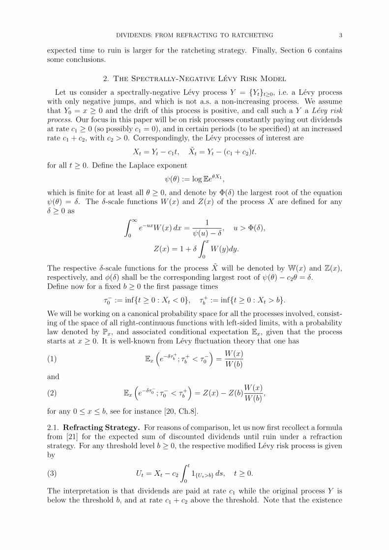
cf. also [18, p.59]. Figure 8 depicts the behaviour of these two quantities as a function of bfor initial capital x = 1 and parameters c = 6, c1 = c2 = 2, λ = α = 1. One observes thatthe expected ruin time (given ruin occurs in finite time) is, for the same barrier, typicallylarger for the ratcheting case, which at first sight may look counter-intuitive, since therefraction strategy increases the drift again when the process is below b. However, thisindicates that in the refraction case those sample paths that do not lead to ruin quickly,will more likely escape ruin also later, so the conditioning on the event of ruin is essentialhere.

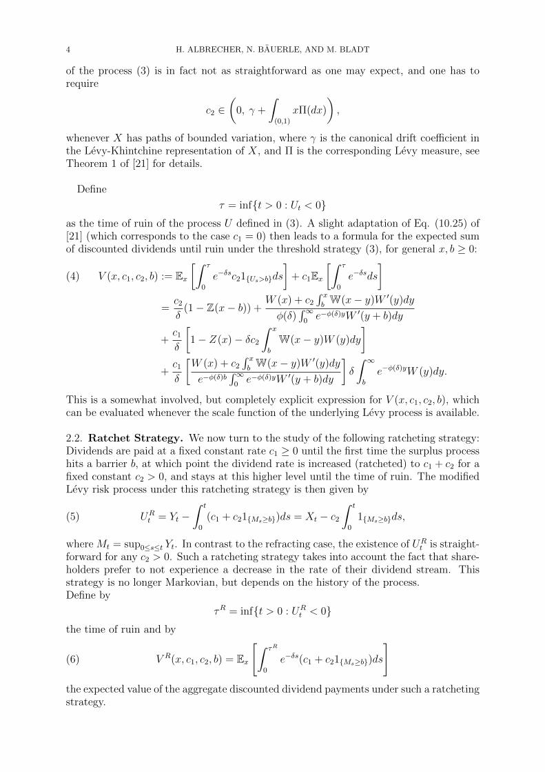
Finally, we compare these properties of sample paths for the refracting and ratchetingstrategies when the respective optimal barrier is chosen. Figure 9 shows the probabilityto reach the optimal barrier before ruin as well as the expected time to reach the optimalbarrier, given that it is reached before ruin for the two strategies, as a function of initialcapital x. Note that for the used parameters, the respective optimal barrier levels arebR = 4.604602 and b∗ = 2.723496. One observes that the despite the higher value of bR,the probability to reach that level (and hence the probability to increase the dividendrate) is not much less than for the respective refraction strategy, whereas the expectedtime to get there roughly doubles.


2 4 6 8 10 12 14b

0.4

0.6

0.8

1.0

1.2

1.4

1.6

Mean

Figure 8. The expected time to ruin, given that it occurs, for the ratch-eting (solid line) and the refracted (dashed line) strategies as a function ofbarrier level b (x = 1, c = 6, c1 = c2 = 2, λ = α = 1).

1 2 3 4 5x

0.75

0.80

0.85

0.90

0.95

1.00

Probability

1 2 3 4 5x

0.2

0.4

0.6

0.8

1.0

1.2

1.4Mean

Figure 9. The probability of hitting the optimal barrier before ruin (left)and the expected hitting time of the optimal barrier, given that it happensbefore ruin (right) as a function of initial capital x, for ratcheting (solidline) and refracting (dashed line), c = 6, c1 = c2 = 2, λ = α = 1.

Remark 5.1. Observe that, as a corollary of the first formula in Example 5.1, by takingthe limit to the diffusion process (10) with drift µ and variance σ2 (using the parametriza-tion (35)) as well as taking b→∞, one retrieves the simple expression

Ex(τ−0 |τ−0 <∞) =x

µ.

Since this formula is interesting in its own right, and seems not to have been consideredin actuarial circles before, we derive it here also directly using an alternative approach.Consider St = x − Yt = −µt − σBt, with drift −µ. By exponential tilting by θ we havethat in the new measure P the process S has drift −µ+ θσ2 and the likelihood ratio

exp(θSt − tψ(θ)) = exp(θSt − t(−µ+ θσ2)θ − tσ2θ2/2)

is a martingale wrt Px, the law of Yt starting at zero, where ψ is the Laplace exponentgiven as in the beginning of Section 2 (here with respect to Px). Inserting now θ = µ/σ2

simplifies to zero drift and

exp(θSt − tψ(θ)) = exp((µ/σ2)St − tµ2/(2σ2)).

Optional stopping holds for this martingale if and only if the stopping times are finite(see e.g. [4, Ch.IV.4]), and the time of ruin τ−0 is such a time, since under Px the drift is


zero. Hence we have

Ex(exp((µ/σ2)Sτ−0 − τ−0 µ

2/(2σ2))) = 1.

But Sτ−0 = x, and

exp((µ/σ2)x− τ−0 µ2/(2σ2))

is bounded around any finite neighbourhood of µ, hence uniformly integrable for anysequence µn → µ so we may take the derivative with respect to µ and get

Ex({

x

σ2− τ−0 µ

σ2

}exp((µ/σ2)x− τ−0 µ2/(2σ2)

)= 0.

This translates in the original measure to

Ex({

x

σ2− τ−0 µ

σ2

}; τ−0 <∞

)= 0,

and a rearrangement yields indeed

x

µ=

Ex(τ−0 ; τ−0 <∞)

Px(τ−0 <∞)= Ex(τ−0 |τ−0 <∞).

6. Conclusion and Future Research

In this paper we considered a ratcheting dividend strategy in an insurance risk theorycontext, where the dividend rate can be raised once during the lifetime of the surplusprocess. We derived analytical formulas for the expected discounted dividend paymentsuntil ruin for a general Levy risk model, and refined the results for a diffusion approx-imation and a compound Poisson model with hyper-exponential claims. The numericalillustrations indicate that the performance of such a ratcheting strategy is in fact notfar behind the optimal refraction strategy, and also in terms of expected ruin time theresulting performance seems rather competitive.There are many possible directions for extensions and generalizations from here. In afuture paper we will consider the case of multiple barriers, where the ratcheting strat-egy will mean a gradual increase of the dividend rate. Another question of interest isto analytically show that the performance of the racheting strategy is monotone in thechoice of the dividend rate increase c2 at the switching time. Finally, to solve the generalstochastic control problem of identifying the optimal ratcheting strategy (which possiblyleads to a continuous function c(x) as a function of first hitting of the surplus level x)will be an interesting challenge for future research.

Acknowledgement. The first author gratefully acknowledges financial support bythe Swiss National Science Foundation Project 200021 168993.

References

[1] H. Albrecher, N. Bauerle, and S. Thonhauser. Optimal dividend-payout in random discrete time.Statistics & Risk Modeling, 28(3):251–276, 2011.

[2] H. Albrecher and A. Cani. Risk theory with affine dividend payment strategies. In Number Theory–Diophantine Problems, Uniform Distribution and Applications, pages 25–60. Springer, 2017.

[3] H. Albrecher and S. Thonhauser. Optimality results for dividend problems in insurance. RACSAM-Revista de la Real Academia de Ciencias Exactas, Fisicas y Naturales. Serie A. Matematicas,103(2):295–320, 2009.

[4] S. Asmussen and H. Albrecher. Ruin probabilities. World Scientific Publishing, Hackensack, NJ,second edition, 2010.

[5] S. Asmussen and M. Taksar. Controlled diffusion models for optimal dividend pay-out. InsuranceMath. Econom., 20(1):1–15, 1997.


[6] S. Asmussen and M. Taksar. Controlled diffusion models for optimal dividend pay-out. InsuranceMath. Econom., 20(1):1–15, 1997.

[7] B. Avanzi. Strategies for dividend distribution: a review. N. Am. Actuar. J., 13(2):217–251, 2009.[8] B. Avanzi and B. Wong. On a mean reverting dividend strategy with Brownian motion. Insurance

Math. Econom., 51(2):229–238, 2012.[9] P. Azcue and N. Muler. Stochastic optimization in insurance. SpringerBriefs in Quantitative Finance.

Springer, New York, 2014.[10] N. Bauerle and A. Jaskiewicz. Risk-sensitive dividend problems. European J. Oper. Res., 242(1):161–

171, 2015.[11] N. Bauerle and A. Jaskiewicz. Optimal dividend payout model with risk sensitive preferences. In-

surance Math. Econom., 73:82–93, 2017.[12] B. de Finetti. Su un’impostazione alternativa della teoria collettiva del rischio. Transactions of the

15th Int. Congress of Actuaries, 2:433–443, 1957.[13] P. H. Dybvig. Dusenberry’s ratcheting of consumption: optimal dynamic consumption and invest-

ment given intolerance for any decline in standard of living. The Review of Economic Studies,62(2):287–313, 1995.

[14] H. U. Gerber. Entscheidungskriterien fuer den zusammengesetzten Poisson-Prozess. Schweiz. Aktu-arver. Mitt., (1):185–227, 1969.

[15] H. U. Gerber and E. Shiu. On optimal dividend strategies in the compound Poisson model. NorthAmerican Actuarial Journal, 10(2):76–93, 2006.

[16] H. U. Gerber and E. S. Shiu. On optimal dividends: from reflection to refraction. Journal of Com-putational and Applied Mathematics, 186(1):4–22, 2006.

[17] H. U. Gerber and E. S. Shiu. On optimal dividends: from reflection to refraction. Journal of Com-putational and Applied Mathematics, 186(1):4–22, 2006.

[18] H. U. Gerber and E. S. W. Shiu. On the time value of ruin. N. Am. Actuar. J., 2(1):48–78, 1998.With discussion and a reply by the authors.

[19] M. Jeanblanc-Picque and A. N. Shiryaev. Optimization of the flow of dividends. Uspekhi Mat. Nauk,50(2):25–46, 1995.

[20] A. E. Kyprianou. Fluctuations of Levy processes with applications. Universitext. Springer Heidelberg,2014.

[21] A. E. Kyprianou and R. Loeffen. Refracted Levy processes. Annales de l’Institut Henri Poincare,Probabilites et Statistiques, 46(1):24–44, 2010.

[22] X. S. Lin and K. P. Pavlova. The compound Poisson risk model with a threshold dividend strategy.Insurance Math. Econom., 38(1):57–80, 2006.

[23] R. Loeffen. On optimality of the barrier strategy in de Finetti’s dividend problem for spectrallynegative Levy processes. Ann. Appl. Probab., 18(5):1669–1680, 2008.

[24] H. Schmidli. Stochastic Control in Insurance. Springer, New York, 2008.[25] S. E. Shreve, J. P. Lehoczky, and D. P. Gaver. Optimal consumption for general diffusions with

absorbing and reflecting barriers. SIAM J. Control Optim., 22(1):55–75, 1984.

(H. Albrecher) Department of Actuarial Science, Faculty of Business and Economicsand Swiss Finance Institute, University of Lausanne, CH-1015 Lausanne, Switzerland

E-mail address: [email protected]

(N. Bauerle) Department of Mathematics, Karlsruhe Institute of Technology, D-76128Karlsruhe, Germany


(M. Bladt) Department of Actuarial Science, Faculty of Business and Economics, Uni-versity of Lausanne, CH-1015 Lausanne, Switzerland


dividends: from refracting to ratcheting

Documents