Munich Personal RePEc Archive

Dividend Policy in Regulated Firms

rondi, laura and cambini, carlo and bremberger, francisca

and gugler, klaus

June 2013

Online at https://mpra.ub.uni-muenchen.de/48043/

MPRA Paper No. 48043, posted 05 Jul 2013 15:30 UTC

1

Dividend Policy in Regulated Firms

Francisca Bremberger1

WU Vienna University of Economics and Business

Carlo Cambini2

Politecnico di Torino and EUI – Florence School of Regulation

Klaus Gugler3

WU Vienna University of Economics and Business

Laura Rondi4

Politecnico di Torino and CERIS-CNR

June 11, 2013

Abstract

We study the impact of different regulatory and ownership regimes on the dividend policy of

regulated firms. Using a panel of 106 publicly traded European electric utilities in the period

1986-2010, we link payout and smoothing decisions to the implementation of different

regulatory mechanisms (cost plus vs. incentive regulation) and to firm ownership (state vs.

private). After controlling for the potential endogeneity of the regulatory mechanism, our

results show that utilities subject to incentive regulation smooth their dividends less than firms

subject to cost-based regulation and present higher impact effects and target payout ratios.

This suggests that when managers are more sensitive to competition-like efficiency pressures

following the adoption of incentive regulation, they adopt a dividend policy more responsive

to earnings variability and more consistent with optimal cash management. These results,

however, apply only to private utilities. If the state still has ultimate control, smoothing of

dividends remains irrespective of the regulatory mechanism. It seems that corporate

governance (i.e. state control) trumps regulation when it comes to dividend payout policy.

Keywords: Dividends, Lintner model, incentive regulation, electricity

JEL: G35, G38, L51, L94

1 WU Vienna University of Economics and Business, Institute of Corporate Governance, Nordbergstrasse 15, 1090 Vienna, Austria. Tel: + 43-1-31336 5495, Email: Francisca.Bremberger@wu.ac.at 2 Politecnico di Torino, DIGEP, Corso Duca degli Abruzzi, 24, 10129 Torino, Italy. Tel: + 39-0115647292, e-mail: carlo.cambini@polito.it. 3 WU Vienna University of Economics and Business, Institute for Quantitative Economics, Augasse 2-6, 1090 Vienna, Austria. Tel: + 43-1-31336 544. Email: Klaus.Gugler@wu.ac.at 4 Corresponding author: Politecnico di Torino, DIGEP, Corso Duca degli Abruzzi, 24, 10129 Torino, Italy. Tel: +39-0115647232, Email: laura.rondi@polito.it , http://www.ceris.cnr.it/Rondi.htm

2

1. Introduction

One of the most important financial decisions that a firm’s managers face is on the amount

and stability of dividends. Dividends have always been a bit of a puzzle in the theory of the

firm. In the neoclassical world of Miller and Modigliani (1961) ‘‘dividends do not matter’’

which is to say that they drop out as a pure residual, once the optimal level of investment has

been determined. Moreover, dividend smoothing is even more suspect: if one thought of

dividends from the view of optimal cash flow management, one might expect them to be

highly volatile. When profits are high, firms invest more and pay out large dividends. When

profits are low, they cut dividends to maintain working capital. In the long run average

dividend payments would be proportional to average profits, but in the short run they would

bounce around. Thus, from the point of view of cash management, dividend smoothing –

since costly - is a puzzle.

In his seminal study, Lintner (1956) noticed that managers are particularly concerned

with the stability of dividends. Half a century later, managers still appear to believe strongly

that the market puts a premium on firms with a stable dividend policy (Brav et al. 2005).

There have been many explanations of this observation including risk aversion on the part of

investors, lack of investment opportunities or signalling theories (Black, 1976). Recently, a

literature evolved explaining dividend smoothing by agency cost explanations, i.e. dividend

policy as a consequence of the separation of ownership and control (Easterbrook, 1984 and,

for comprehensive empirical evidence, Leary and Michaely, 2011). Agency theory predicts

substantial and stable dividends. The higher dividends are, the less free cash flow there is,

ceteris paribus, in managers’ hands to spend on negative net present value projects. The

higher dividends are, the greater is also the need to go to the capital market for new outside

funds, and the greater the effectiveness of monitoring. If the primary function of dividends is

to force firms into the capital market, regular and stable payouts are more valuable.

Fudenberg and Tirole (1995) explain income and dividend smoothing based on incumbency

rents. If managers enjoy private benefits from being in control, they, individually and

rationally, smooth dividends. In bad times, they pay out too much dividends to lengthen their

tenure. In good times, they are less concerned by their short-term prospects and information

decay allows them to save for future bad times. Finally, La Porta et al. (2000) conjecture that

minority shareholders press corporate insiders to pay dividends, since they cannot be sure to

get a fair return particularly in countries where shareholder rights are not well developed.

Consistent with an agency cost explanation of dividend smoothing, Gugler (2003) finds that

target dividend levels, the smoothing of dividends, and the reluctance to cut dividends depend

3

on the identity of the (ultimately) controlling owner. State-controlled firms engage in dividend

smoothing and have the highest target payout ratios while, in marked contrast, dividend

payments of family-controlled firms are not subject to dividend smoothing. Furthermore,

state-controlled firms are most reluctant to cut dividends while family-controlled firms are

least reluctant to cut dividends. More recently, Michaely and Roberts (2012), finding that

privately owned firms smooth dividends and payout less than their publicly listed

counterparts, suggest that the scrutiny of public capital markets, ownership structure and

incentives altogether play key roles in shaping firm dividend policy.

In this paper we conjecture that there is still another factor that comes into play when

we look at the dividend policy of large firms: regulation. When looking at public utility

services, the state has two options to provide those services. First, the state himself can

provide the services and own the assets so involved. Second, the state can privatise the

companies providing these services and regulation accompanies this process: to prevent the

abuse of natural monopoly positions, regulatory authorities are usually established that subject

the utilities to regulation. An interesting hybrid construct is the partially state-owned company

subject to regulation. The question that arises with such constructs is whether effective

regulation can be expected if the state both owns part of the assets and sets up the regulatory

framework. We analyse such set-ups in the electricity industry. In particular, we compare the

dividend policy of firms that are partly owned by the state and subject to regulation with firms

that are fully private and subject to regulation.

These firms are not only key for national economies in terms of aggregate investment

(Guthrie, 2006) and market capitalisation (Bortolotti, Cambini and Rondi, 2013), they are also

remarkable because of their generous dividend payments. A recent report by J.P. Morgan

(2011) shows that telecom and electric utilities have been the highest-paying industries in the

U.S. in the last years. Dividend payout, i.e. the ratio between dividends and net income, is

118% for telecoms and 56% in utilities, while dividend yield, i.e. annual dividends per share

divided by the share price, is 5.3% for the telecom industry and 4.5% for the other utilities,

which are the highest values among all sectors.

These firms are subject to regulatory oversight, a feature that most of the times has set

them apart when studying dividend policy, the common explanation being that their dividend

behaviour does not reconcile with current textbook explanations because regulated sectors are

less risky, insulated from product and even capital markets’ discipline and where regulators

directly or indirectly may influence how much dividend they can pay. For example Moyer,

Chatfield and Sisneros (1989) find that security analysts’ monitoring activities are lower when

4

the firm is a public utility. In general, the finance literature that examined the dividend

behaviour of regulated firms focused on the role that dividend payouts play in the monitoring

process to reduce equity agency costs within capital markets (Miller, 1986; Smith, 1986; and

Hansen, Kumar and Shome, 1994).

The aim of this paper is to study regulated firms’ dividend policy with a new

perspective that investigates whether different types of regulatory contracts can influence

firms’ smoothing and payout decisions. To this purpose, we examine how firms respond to

changes in regulatory mechanisms that are aimed at enhancing their efficiency as well as at

shaking their “quite life”. Since the European energy sector has been subject to significant

regulatory and privatisation reforms, we use a large sample of European electric utilities from

1986 to 2010 to link their dividend behaviour to the implementation of new regulatory

mechanisms, allowing for potential influences of their ownership status. Moreover, this paper

also departs from the previous literature in that we account for the potential endogeneity of

the regulatory policy.

Over the last thirty years, the EU energy sector underwent many reforms, mainly

aimed at liberalising the market and at privatising the state-owned monopolies. The main

purpose was (and still is) to raise firm efficiency and to improve the quality of service. While

electric generation is already almost fully liberalised (and de-regulated) as well as privatised

in most EU countries, transmission and distribution services are still subject to regulation

either by independent regulatory agencies or by executive-branch commissions, and many

transmission and distribution operators still remain partially (or fully) controlled by the state.5

Among market reforms that affect the provision of public utilities, the choice of the

regulatory contracts is a key policy decision that in many countries has brought the

implementation of modern regulatory mechanisms (Laffont, 1994): incentive regulation.

Incentive regulation serves the purpose to raise the efficiency of energy utilities that had so far

been regulated – both in the US and in Europe - through a cost-based regulatory mechanism.

Mainly adopted to reduce managerial slack, these modern regulatory schemes are thought to

provide powerful incentives to increase efficiency by leaving larger profits to the regulated

operator. At the same time, earnings become more volatile and firms under incentive

regulation are perceived to be riskier by the financial markets.6

Starting from the classic Lintner model, we modify the standard partial adjustment

specification to take into account the potential effect of a regulatory policy change on firms’

5 For an overview of the regulatory and privatisation reforms in the European electric sector, see Cambini, Rondi and Spiegel (2012). 6 See the surveys by Armstrong and Sappington (2006 and 2007) and Joskow (2007).

5

dividend behaviour. We argue that, under cost-based regulation, the regulated price moves

with ex post costs which is why the firm has more stable cash flows, whereas under incentive

regulation profits mostly depend on the firm’s ability to achieve efficiency gains; hence firms

are the “residual” claimants. The pressure to increase efficiency is stronger under incentive

than under cost-based regulation, which should drive the behaviour of incentive regulated

firms to smooth their dividends less than firms under cost-based regulation. Dividend flows

are therefore likely to be more stable for firms under cost-based than under incentive

regulation.

The reluctance of the national governments to release control and ownership of energy

incumbents may be, in part, related to the reluctance to abandon the large dividend rights that

accrue to the state as the main shareholder. Especially when the budget constraint tightens (as

in the recent years in all Western economies), the “energy dividend” becomes a more or less

safe and steady source of financing. Our next research question therefore asks whether the

firm’s ownership structure may also affect the dividend policy of electric utilities. We argue

that the reasons why ownership is expected to matter for regulated firms’ dividend policy are

not only related to the classical agency problem as developed by Gugler (2003) or Michaely

and Roberts, 2012), but also to government and political interference in utilities’ real and

financial decisions (Shleifer and Vishny, 1994; Shleifer, 1998; Bennedsen, 2000; and, for an

empirical test on European firms, Bortolotti, Cambini and Rondi, 2013).

Our results show that, consistent with our theoretical model, the dividend behaviour of

incentive and cost-based regulated utilities differs significantly. Throughout most

specifications and econometric methods, electric utilities under incentive regulation are found

to exhibit lower smoothing parameters and higher impact effects. Moreover, higher target

payout ratios for incentive regulated firms are found in all GMM specifications. However,

these results are only valid when the firms are privately controlled. In marked contrast,

partially-state owned firms actually display larger smoothing of dividends when incentive

regulation is introduced, while impact effects are unaltered, compared to state-controlled

firms under cost-based regulation. This leads to a rise in target payout ratios for state-

controlled firms under incentive regulation. These results suggest that incentive regulation

transfers more risk to regulated firms, making their managers more sensitive to competition-

like efficiency pressures, hence more likely to cut dividends when necessary, when also

control is privatised. If control remains in state-hands, the effects of regulatory reform differ,

at least with respect to dividend policy.

6

To the best of our knowledge, this paper is the first systematic analysis of the

interrelation between regulation, ownership and dividend payout policy. The outline of the

paper is the following. In Section 2 we present the dividend model of smoothing and payout

extended to account for regulatory regimes and we describe our estimation strategy. Section 3

describes the changing pattern of the regulatory framework in the European energy market,

the sample and the data we use for the estimations. In Section 4 we present the main results.

Section 5 summarises and concludes.

2. Research Design and Estimation Strategy

2.1 A Model of Dividend Policy for Regulated Firms

We start by assuming that firms set their dividend payout policy according to the partial

adjustment model of Lintner (1956). Following the Lintner Model, dividends are the result of

a partial adjustment of last year’s dividends towards a target payout ratio. In more details, for

any year t, the target level of dividends, *itD for firm i, is related to the current earnings, itE ,

through a desired payout ratio τi:

itiit ED τ=* (1)

In any given year the firm will only partially adjust their dividend policy towards the

target dividend level. Hence, it results:

itititiiitit uDDaDD +−+=− −− )( 1*

1 α (2)

where 1−− itit DD is the actual change in the dividend, ai is a constant, αi measures the speed

of adjustment and lies between zero and one, and 1*

−− itit DD is the desired change in the

dividend. The closer αi is to one, the faster the speed of adjustment is. (1 - αi) is called the

Smoothing parameter, and τi is the Target Payout Ratio parameter, which gives the optimal

percentage of profits for distribution via dividends. The constant term ai is generally positive

and it reflects the greater reluctance to reducing vis-à-vis raising dividends, which is

commonly observed. Finally, uit represents the discrepancy between the observed change and

that expected on the basis of the model. The adjustment process can be rewritten as:

7

ititiitiiiit uDEaD +−++= −1)1( ατα (3)

where i i

α τ , the coefficient on current earnings, is called the “impact effect”. This

leads to the following empirically testable equation:

itititiit uDEaD +++= −121 ββ (4)

and computation of the three parameters of interest, smoothing, impact effect and target

payout ratio, as follows:

12 1

2

1 ; ; 1

i i i i

βα β τ α β τβ

− = = =−

(5)

Recent empirical analyses on dividend policy show that dividend smoothing is highly

affected by earnings volatility and company risk. In particular, Leary and Michaely (2011)

empirically find that firms with high earnings and cash flow volatility, and therefore more

risk, tend to smooth less. We directly incorporate this empirical evidence in our setting

modifying the measure of the speed of adjustment in the following way:

(1 )i i i

α α σ= +

where αi is again the standard measure of the speed of adjustment, and σi is a measure of the

earnings volatility of firm i. This assumes that the speed of adjustment increases as long as

earnings volatility rises, and implies that we can rewrite Equation (2) as follows:

itititiiitit uDDaDD +−+=− −− )( 1*

1 α

with itiit ED τ=* . This leads to the following:

1(1 ) (1 (1 ))it i i i i it i i it it

D a E D uα σ τ α σ −= + + + − + +

This implies that the “adjusted” smoothing parameter becomes:

8

2ˆ 1 (1 ) i iα σ β− + = . (6)

Condition (6) shows that higher earnings volatility leads to a smaller smoothing

parameter, in line with evidence by Leary and Michealy (2011).

We believe that this approach is particularly important in explaining dividend

decisions in regulated utilities where earnings volatility is strongly correlated with the kind of

regulatory contracts firms are subject to. The different contractual regimes adopted to regulate

utilities all over the world range from the standard low powered incentives/cost-based

mechanism – such as the rate of return regulation - to the more recent incentive regulatory

schemes - such as the revenue or price cap mechanisms (see Laffont, 1994; Armstrong and

Sappington, 2006 and 2007). To this aim, it is important to recall the scope and the effect of

the introduction of different contractual types on firm performance.

The most famous cost-based regulatory mechanism is known as the rate of return

regulation, whereby regulators fix the rate of return the utility can earn on its assets. With this

form of contract, the regulators set the price the utility can charge so as to cover all main

operating costs and to allow it to earn a specified rate of return. The regulated price can then

be adjusted upward (downward) if the firm starts making a lower (higher) rate of return. In

turn, this implies that this pricing scheme not only does not boost firm efficiency but it also

reduces earnings volatility and guarantees financial integrity of the regulated firm (Armstrong

and Sappington, 2006; Joskow, 2007).

Contrary to the standard cost-based mechanism, the purpose of incentive regulation is

to encourage efficiency gains. By pursuing cost savings, managers can generate higher profits

and thus benefit shareholders. However, incentive schemes change over time and are

generally revised periodically by national regulators to avoid the regulated company to earn

supernormal profits. This implies that the firms can maintain high profits only if the

management succeeds in seeking out further cost savings. Incentive regulation7 may thus

leave excess profits to the regulated operator, if the firm is able to meet the incentives set by

the regulators constantly over time; but its adoption also shifts the risk of demand or cost

fluctuations on the firm, increasing therefore the variability of the company earnings. Indeed,

empirical evidence shows that on average the adoption of incentive mechanisms not only

7 Incentive regulation is usually implemented as price- or revenue-cap mechanisms or benchmarking (Littlechild, 1983), through the application of fixed-price contracts (Armstrong and Sappington, 2007). Sappington (2002) is a comprehensive survey of incentive regulation mechanisms and instruments. Joskow (2008) surveys incentive regulation schemes as adopted in the energy industry.

9

leads to higher productivity but also to higher net profits (Ai and Sappington, 2002), higher

volatility in earnings (Parker, 1997)8 and higher systematic risk (Alexander and Irwin, 1996;

Grout and Zalewska, 2006) than the standard low-powered incentive cost-based mechanism.

From the above analysis, we therefore have the following testable hypothesis:

H1 (Dividend Smoothing): Firms under Incentive Regulation have

lower smoothing parameters than firms under Cost-Based regulation.

Thus, we argue that, under cost-based regulation, the regulated price moves with ex

post costs which is why the firm has more stable cash flows, whereas under incentive

regulation, profits mostly depend on the firm’s ability to achieve efficiency gains; hence firms

are the “residual” claimants. Dividend flows are therefore likely to be more stable for firms

under cost-based than under incentive regulation. The pressure to increase efficiency is

stronger under incentive regulation than under cost-based, which should drive the behaviour

of incentive regulated firms to smooth their dividends less than firms under cost-based

regulation.

However, there is one big qualification to this hypothesis, namely whether continuing

state-control counteracts the efficiency effects of incentive regulation. Elected politicians are

held accountable for all of the activities of government. They can be expected to have a

particularly strong interest in seeing a steady flow of dividends from a company controlled by

the state, since (1) dividends may suffice to convince citizens that the company is performing

well, and (2) a steady stream of dividends reduces the cash flow in the hands of the managers

(see Gugler, 2003). (3) The reluctance of the national governments to release control and

ownership of energy incumbents may be, in part, related to the reluctance to abandon the large

dividend rights that accrue to the state as the main shareholder.9 Especially when the budget

constraint tightens (as in the recent years in all Western economies), the “energy dividend”

becomes a safe and steady source of financing.

Our next research question therefore asks whether the firm’s ownership structure may

also affect the dividend policy of electric utilities. In particular, we expect that state-controlled

firms continue to smooth their dividends despite of incentive regulation, since politicians

8 Parker (1997) shows that after the introduction of incentive regulation profits of many UK utilities largely increase but they also start to fluctuate a lot both in the electricity and telecom sectors. On the contrary, in the gas industry the incumbent operator British Gas presented falling profits over time due to large restructuring costs and the excessive costs of the contracts for gas provision. 9 There are several recent examples for this. Verbund, for example, a large Austrian electricity company left its dividend stable in 2011 despite a slight drop in profits (see Stock-Express.Com, 29 February, 2012). Verbund is 51% state controlled. The management of Verbund aims at a “target 50% payout ratio”. 

10

and/or controlling bureaucrats demand stable dividends. After all, (excessive) dividends, i.e.

rent extraction from producers and/or consumers, represent a much more hidden way of

increasing the funds available for politicians than direct taxation.

If incentive regulation leads to larger efficiency pressure, cash management should

(must) also be optimised. If profits are high, dividend payouts should be high, if profits are

low, dividend payouts should be low. Moreover, note that according to Moyer et al. (1992)

regulated utilities use dividend payouts as a strategic instrument to obtain more favourable

conditions on retail prices from the regulator. Hence, utilities may use their earnings to

distribute larger payouts to affect the regulatory policy.10

We thus claim that the type of the regulatory contract also allows us to hypothesize on

the impact effect.

H2 (Impact Effect): Firms under Incentive Regulation have larger

impact effect parameters than firms under Cost-Based regulation.

Again, this analysis is largely confined to private firms. If incentive regulation does

not imply the same efficiency and/or strategic implications for state-controlled firms than for

private firms, we would also not expect hypothesis 2 to hold for them.

Previous studies (Moyer et al., 1992; Hansen et al., 1994) show that payout ratios of

regulated utilities are typically higher than payout ratios for non-regulated industrial firms.

According to these studies, regulatory oversight from national regulators insulates utility

managers from the discipline of both the market for corporate control and the product market

competition. However, while these factors help to explain why larger payout ratios are

expected in utilities, they are not sufficient to explain the variation in dividend payouts across

utilities.

The hypothesised effects of incentive regulation on the target payout ratio are more

subtle. On the one hand, incentive regulation should reduce dividend smoothing, leading to

lower target payout ratios, on the other hand the increased efficiency and/or strategic

pressures of incentive regulation should lead to larger impact effects, and thus to larger target

payout ratios (see equations (5)). Thus, ex ante we cannot determine which effect is larger,

and we leave this to the empirical analysis. While the same arguments may apply to state-

controlled companies, one may argue that their target payout ratios unambiguously increase

under incentive regulation. The reasons are that the rents so extracted from producers and/or

10 This is in line with the strategic use of leverage already shown in previous studies (Daspupta and Nanda, 1993; Bortolotti et al., 2011).

11

consumers are a more opaque way to increase funds for politicians than direct taxation, and,

what is more, high and stable dividends may be taken as a signal that the state-controlled

companies are performing well and increase efficiency under incentive regulation.

2.2 Estimation Strategy

The theoretical framework developed in the previous section provides the hypotheses

to be tested by our econometric analyses. Estimation of the Lintner partial adjustment model

using panel data raises a number of econometric problems that only recently have been

explicitly addressed and accounted for (see for example, Andres et al., 2009, and Khan,

2006). The first estimation problem is that the Net Profits (or Cash Flows) variable is likely to

be correlated across firms with the firm-specific effect and that the lagged Dividends variable

is most likely correlated with these firm-specific effects. To remove the firm-specific effect,

the within-group estimator can be used, but then, because the fixed-effect transformation

requires time-demeaning of all variables, the lagged dependent variable would remain

correlated with the transformed disturbance term. To obtain consistent estimators, we thus

use the first-difference transformation to eliminate the fixed effect and then apply the linear

generalised method of moments (GMM) estimator developed by Arellano and Bond (1991)

and Arellano and Bover (1995). This estimator is especially designed for panel data models

where the lagged dependent variable is included and some of the regressors are potentially

endogenous and lagged values of the dependent variable can be used as instruments, provided

there is no serial correlation in the disturbance. More specifically, we use the dynamic

System-GMM estimator (Arellano and Bond, 1991, and Blundell and Bond, 1998), which

deals with situations where the lagged dependent variable is persistent (i.e. the autoregressive

parameter is large).11

We modify the original Lintner model so as to allow for a change in dividend

behaviour due to the regulatory regime, interacting both the lagged dividend and

contemporaneous profits with a binary variable Inc Reg it, which is equal to 1 when the firm is

11 This model estimates a system of first-differenced and level equations and uses lags of variables in levels as instruments for equations in first-differences and lags of first-differenced variables as instruments for equations in levels, for which the instruments used must be orthogonal to the firm-specific effects. For the validity of the GMM estimates it is crucial that the instruments are exogenous. We check that they are and report the appropriate tests: the Arellano and Bond (1991) autocorrelation tests to control for first-order and second-order correlation in the residuals, the two-step Sargan-Hansen statistic to test the joint validity of the instruments and the Difference-in-Hansen test of exogeneity of individual instruments to test the overidentifying restrictions for the external instruments. The Sargan-Hansen test is robust, but may be weakened if there are too many instruments with respect to the number of observations (see Roodman, 2006). Therefore, we follow a conservative strategy using no more than two lags of the instrumenting variables, so as to assure that the number of instruments is not greater than the number of firms. Standard errors are robust to heteroskedasticity and arbitrary patterns of autocorrelations within individuals.

12

regulated by an incentive mechanism (price- or revenue-cap, or benchmarking), and 0 when a

cost-based regime is in place. The estimation equation is therefore:

0 1 1 2 1 1 3 4it i i it i it it i it i it it itD a a D a D Inc Reg a E a E Inc Reg ε− − −= + + + + + (7)

A further econometric issue is the potential endogeneity of the regulatory contracts –

low vs. high-powered incentive schemes - that is chosen by the regulator. Ideally, to deal with

the endogeneity of the contract type within a static setting, we might use a standard

instrumental variable estimator (as in Bortolotti, Cambini and Rondi, 2013, for a market-to-

book regression model), but the presence of the lagged dependent variable, and the need to

deal with the dynamic panel bias, rules out the 2SLS approach. Within the GMM framework

we can also GMM-instrument the interacted Inc Reg, on the ground that the “contract type” is

fundamentally a choice variable that arises through a process of bargaining between the

regulator, the firms and eventually the government,12 where this bargaining process is

influenced by the past performance (dividends and profits) of the firm (as in Wintoki, Linck

and Netter, 2012). In addition, we can also count on external instruments and use a set of

variables that account for domestic institutions and country specific features to instrument Inc

Reg. For this purpose, we rely on characteristics that may influence the choice of a regulatory

regime, and use country-specific, time-varying variables extensively used in the applied

political economy literature and typically sourced from the World Bank database on Political

Institutions (see Beck et al., 2001, for a detailed description of the variables). Herfindahl

Gov., the Herfindahl Index Government, is the sum of the squared seat shares of all parties in

the government and is expected to control for the internal cohesion of the executive hence the

ability to make and enforce policy decisions. ORIENTATION is a time-varying variable

which accounts for the political orientation of the executive in charge; it is equal to 1 when

the executive is rightwing, 2 when it is centre, and 3 when it is leftwing. STABILITY is a

survey-based measure that captures the extent of turnover of a government's key decision

makers in any year and ranges from 0 (high stability) to 1 (low stability). CHECKS is an

index for checks and balances incorporated into a political system that ranges from 1

(minimal checks) to 10 (maximal checks).

12 This view is consistent with the theoretical analysis by, for example, Besanko and Spulber (1992) and by anectodal evidence. In particular, according to the U.S. Supreme Court, the decision to adopt a specific regulatory contract “involves a balancing of the investor’s and the consumers’ interests” that should result in rates “within a range of reasonableness” (see Federal Power Comm. v. Hope Natural Gas Co., 320 U.S. 591, 603 (1944)).

13

Finally, we include firm ownership, in the form of a dummy, State Control, which is

equal to 1 when the government directly and/or indirectly holds at least 25% of the firm

ownership, and has therefore ultimate control. This variable is original and manually

constructed by the authors, as further detailed in the data section below.

The role of firm ownership, and particularly state ownership, is multifaceted because it

may be viewed as affecting both dividend (Gugler, 2003) and regulatory policies. We have

noted that privatisation of transmission and distribution operators is far from complete and

this reluctance to privatise for governments with tight budget constraints and rocketing debt-

to-GDP ratios may be attributed to the substantial dividends that these operators distribute.

However, insofar as firm value is the present value of the stream of future dividends, the

decisions whether to sell the firm now or to cash in the dividends forever only depends on the

government’s preference for privatisation proceeds vis-à-vis an ongoing stream of dividends.

Conversely, to the extent that the government can interfere with regulatory decisions (such as

the choice of the regulatory institution or of the regulatory mechanism, down to setting the

regulated rates) to obtain a more favourable treatment for state controlled firms that results in

a large dividend payout, state ownership can be viewed a key determinant of regulation

policy. Thus, eventually, state ownership potentially should matter for dividend policy both

directly via state-control of the company and indirectly via regulatory policy. In a first step,

therefore, we use State Control as an instrument for Inc Reg, thereafter we additionally

include State Control as a direct determinant of dividend payout policy.

To summarise we start by presenting the results from simple pooled-OLS regressions

(with time dummies), and then proceed with fixed-effect estimates before turning to two sets

of GMM-IV results. In the first set, in order to allow for the endogeneity of regulatory regime,

we GMM instrument not only the lagged Dividends but also its interaction with Inc Reg; in

the second one, we also account for the potential influence of domestic institutions on the

choice of the regulatory policy and, accordingly, introduce a set of external instruments drawn

from the recent political economy literature. In a last step, we look whether state control has

also a direct effect on dividend payout policy.

For robustness, we repeat the empirical strategy using Cash Flows instead of Net

Profits as suggested by Fama and Babiak (1968) and recently adopted by Andres et al. (2009).

Our panel includes firms from several countries with different and time-varying tax laws with

respect to fixed assets depreciations (equipment write-offs and allowances for accelerated

depreciations which may be relevant for capital intensive electric utilities) as well as to legal

reserves. With this alternative approach we try to allow for dividend decisions that are not

14

based on published earnings only. Since results are very similar and robust, we confine the

Cash Flow results to the appendix.

3. Institutional Context, Data and Summary Statistics

3.1. Institutional Context

In the last decades, the European Commission issued several directives in order to prompt

national reforms that redesigned the legal and regulatory framework in the public utility

sector, and in particular in the electricity industry. While until the early nineties, public

utilities in Europe, with the only UK exception, were characterized by vertical integration,

state monopoly and public ownership, the aim of such reforms was to raise efficiency,

improve service quality, and spur infrastructure investment through the introduction of

liberalization, privatization and new regulatory interventions.

Directive 96/92/EC built the basis for this significant reform of the European

electricity market. Its main aim was to open national electricity markets and to prepare an

integrated electricity market in Europe. The directive contained common rules for electricity

generation, transmission and distribution, in order to induce convergence in production and in

market structures in single member states. In addition to that, monopolistic (transmission and

distribution) and potential competitive markets (generation and retail) were distinguished and

member states were required to establish independent transmission grids. Directive

2003/54/EC, the acceleration guideline, required complete opening of national electricity

markets by July 1st, 2007. Moreover, legal unbundling and an independent national regulatory

authority were demanded for the first time. The third energy package, Directive 2009/72/EC,

further increased the unbundling requirements. Member countries can now choose between

three different unbundling models: ownership unbundling, an independent system operator or

an independent transmission operator. Although the effects of the different unbundling

methods are still discussed, most European countries already switched to ownership

unbundling.

According to the EU legislator, privatisation and liberalisation should enhance

efficiency and competition, reduce the consumer’s dependency on few large suppliers and

increase security of supply. With reference to firm ownership energy enterprises, the

European Union encouraged member states’ governments to shift from the classical vertically

integrated and state-controlled set-up towards unbundling and (at least partial) privatisation.

15

However, the EU Commission left the ultimate decision about utilities’ ownership entirely in

the hands of national governments. As of 2012, privatization of public utilities within EU

member states is far from complete, and central and local governments still hold majority and

minority ownership stakes in many regulated utilities, particularly in Austria, France, Finland,

Germany and Italy.

Concerning the regulatory framework for setting trasmission and distribution charges

most of the European countries (except for the UK) initially started with a cost-based

regulation. Nevertheless, switching to some kind of incentive regulation has been part of most

regulatory reform processes worldwide (Vogelsang, 2002; Cambini and Rondi, 2010). The

EU Directives did not impose any mandatory rule on the form of regulatory schemes,

delegating the choice of the most appropriate regime to each national regulatory agency. For

this reason, the regulatory mechanisms differ across countries and across market segments.

They range from the typical cost-plus (mainly, rate of return) to incentive-based schemes,

either in the form of price or revenues caps or through benchmarking (yardstick) competition.

Within the electricity sector, the UK adopted incentive mechanisms in the early nineties in

both distribution and transmission, while other countries - like Belgium, Hungary, Italy, Spain

and Norway – switched later from rate of return to incentive based pricing in both segments.

Austria, Denmark, Finland and Sweden shifted to incentive schemes only in distribution,

Greece and France still rely only on cost-plus mechanisms while Germany switched to

incentive regulation in 2010.

Figure 1 presents a timeline indicating the first introduction of incentive regulation in

the electricity market (for distribution, transmission or both) of several European countries.

Figure 1: Timeline of the Introduction of Incentive Regulation

16

3.2 Data and Summary Statistics

The starting point of our sample creation were all firms listed in Worldscope, with a primary

or secondary SIC code equal to 4911 “Electric services”.13 We reviewed the selected sample

by checking all included firms by hand and eliminating the ones which are mainly operating

in different fields, like conglomerates or investment trusts. Subsequently, we created a

dummy indicating whether the firms operate in distribution, transmission or production of

electricity. We dropped all firms that are exclusively operating in electricity production,

because these firms are not subject to regulation.

Finally, we obtain an unbalanced panel sample consisting of 106 firms operating in the

European14 electricity market in the period of 1986 to 2010. We use total common and

preferred dividends paid to shareholders as dividend variable Dividends. For current earnings

we use two different proxies: net income after preferred dividends for Net Profits of the firms

and net profits plus depreciation, depletion and amortisation for Cash Flows of the firm (see

the appendix). All variables are recorded in US$, see Table 1 for definitions of all variables

used.

To describe the regulatory regime the firms are facing, we constructed a dummy for

incentive regulation (Inc Reg). This dummy contains a one if either transmission or

distribution operates under incentive regulation, zero otherwise. The incentive regulation

dummy is on the one hand used to create interaction terms with the main explanatory

variables current earnings and lagged dividends and on the other hand for sub-sampling.

Concerning the ownership data we constructed a dummy (State Control), indicating at least

25% state ownership. This threshold was chosen because 25% of shares establish a blocking

minority in most European countries, which enables the owner to control important, strategic

decisions of the enterprise. In creating the dummy we took the following procedure: If the

state (governments at federal, state and local level) holds 25% or more of the shares of a firm,

the dummy contains a one, zero otherwise. If a so state-controlled firm holds the majority of

shares of another firm, this second firm is also marked as state-controlled. In that, direct and

ultimate state ownership are considered. The necessary information was mainly collected

from the homepages and annual reports of the firms.

13 If a sales breakdown for segments is available SIC Code 1 would represent the business segment which provided the most revenue, and SIC Code 2 the second most. If a sales breakdown is not available the SIC Code is assigned according to the best judgment of Worldscope (Worldscope Database – Datatype Definitions Guide). 14 Included countries: Austria, Belgium, Czech Republic, Denmark, Finland, Italy, Luxembourg, Norway, Poland, Portugal, Spain, Sweden, Switzerland, United Kingdom.

17

Table 2 summarises descriptive statistics of all variables included in the regression

analysis for the full sample (Panel A), highlights the yearly development of Inc Reg and State

Control (Panel B), and presents means and mean difference tests in the variables between the

different regulatory regimes (Panel C).

As reported in Panel A, firms pay on average around 230 Mio USD in Dividends out

of Net Profits of 384 Mio USD (and Cash Flows of around 900 Mio USD). Around 33% of

firm-years operate under incentive regulatory schemes, while 67% under cost-based type

regimes. However, over time 74 out of the 106 firms face a regulatory regime switch from

cost-based to incentive regulation. The average country in the sample locates around the

centre of the political spectrum (mean Orientation of 2.05), enjoys broad internal cohesion in

government (mean Herfindahl Gov. of 0.66), with a Checks average of around 4.19 (out of a

maximum of 10), and faces political stability (mean Stability of 0.14). More than half of the

firm-years (56.5%) are under state control, and over time 28 out of the 106 firms face a switch

in State Control.

A comparison of incentive versus cost-based regulated firms is particularly revealing

(see panel C). Interestingly, if there is cost-based regulation in place, the percentage of

companies still ultimately controlled by the state is much higher (68.7%) than if incentive

regulation is in place (34.8%). Moreover, over time, incentive regulation gains and cost-based

regulation looses importance, while the state gradually withdraws from control over time (see

Panel B). This is a first indication that regulation and ownership/control are related.

3.3. Profitability, Dividends and Volatility across Regulatory Regimes

Our theoretical framework highlights the impact of earnings (profitability) variability and firm

risk on dividend smoothing, while hinting at the potential differences of returns volatility for

utilities operating under cost-based or incentive regulation. Thus, before turning to the

estimation of the modified Lintner dividend model, we present evidence of firm heterogeneity

of the level and variability of profitability and dividend payout across regulatory regimes (for

a similar approach see for example Leary and Michaely, 2011, and Michaely and Roberts,

2012 and, specifically on regulated electric utilities, Hansen et al. 1994). We use Net

Profits/Total Assets, Cash Flows/Total Assets, EBITDA/Total Assets (Return on Assets or

ROA) and Net Profits/Equity (Return on Equity or ROE) as profitability measures and, to

gauge dividend policy, we use both Dividend/Net Profits and Dividend/Cash Flows as

measures of payout and Dividend/Total Assets as an alternative normalisation for dividends.

In the lower part of Table 2, Panel C, we use the standard deviations of these variables to

18

measure their volatility. Finally, to further document the differences in return variability (and

firm risk), we include a comparison for Price Volatility, which is a measure of a stock's

average annual price movement to a high and low from a mean price for each year. Figures 2-

4 visually track the evolution over time of selected variables by regulatory regime.

Table 2, Panel C highlights the following differences between the sub-samples of

incentive versus cost-based regulation. First, as already mentioned, the state is much more

important as a controlling shareholder for cost-based regulated firms than for incentive

regulated firms. Second, whether we measure them using Net Profits, Cash Flows or Ebitda,

we find that firms under incentive regulation exhibit significantly higher profitability ratios

than firms under cost-based regulation. This is consistent with the efficiency enhancing

pressures of incentive regulation we hypothesized in the theory section. Third, the picture is a

bit more nuanced with respect to dividend payout ratios. While Dividends as a share of Net

Profits are (insignificantly) lower for incentive regulated firms (53.7%) than for cost-based

regulated firms (55.4%),15 firms under incentive regulation pay out significantly larger shares

as a percentage of Total Assets and Cash Flows. Thus, again consistent with our theoretical

priors, the effects of incentive regulation on the dividend payout ratio are not clear-cut, since

both lower smoothing but higher impact effects may be present at the same time. Finally, all

comparisons of standard deviations of our profitability and dividend measures indicate, that

the volatility of profitability and dividends goes up with the introduction of incentive

regulation. We also find that stock price volatility, a market based proxy for firm risk, is also

(significantly) higher for incentive regulated firms. The graphical evidence is in line with the

mean differences tests. Figure 2 shows that profitability of incentive regulated firms as

measured by the Return to Asset tend to be both higher and more volatile. This pattern is

confirmed by Figure 3, which maps Dividend to Total Asset, and by Figure 4 where we graph

Price Volatility.

Summarising, both the level and variability of profitability go up after the introduction

of incentive regulation. This is consistent with efficiency enhancing pressures and firm

riskiness going up due to becoming a “residual claimant” under incentive regulation. While

this translates into a dividend policy, that is significantly more volatile whenever the firm is

under incentive regulation, the dividend payout ratio does not necessarily go up. Thus, to

ultimately judge the effects of incentive regulation one needs to look at the time profile of

dividend payout policy, which we do below by estimating the Lintner model.

15 Of course, the absolute amounts of dividends are higher under incentive regulation, since profits are so much higher.

19

4. Results

4.1. The Lintner Dividend Model for Regulated Firms

As our unbalanced panel data set comprises different firms as well as varying time

spans between 1986 and 2010, panel regression techniques have to be used to account for the

characteristics of longitudinal data. We concentrate on estimating the pure Lintner Model, not

accounting for other firm-differences (like size or tax differences between countries), which

might be correlated with dividend payouts. Therefore, fixed effects (FE) specifications are

theoretically more convincing than random effects specifications for estimating the Lintner

Model. Moreover, as discussed in Section 3, the own past of dividend payouts is an important

aspect of the Lintner Model for representing the adjustment process towards the target payout

ratio. Including a lagged dependent variable may lead to biased estimates within the usual

fixed effects panel framework. Consequently, although we report for comparison, pooled-

OLS and FE estimates, we focus our presentation of results on the system GMM estimator.

As a starting point, Table 3 reports the results for the full sample (Equation [4]), Table

5 allows for the differential impact of incentive vs. cost-based regulatory regimes by

estimating the unrestricted model in Equation [7], while Table 4 reports the results of a

regression analysis of the determinants of the choice of the regulatory mechanism (our quasi-

first stage analysis). For all tables we quantify and report the corresponding model

parameters: the coefficients of dividend smoothing (S), the impact effects (I) and the

estimated target payout ratios (Tpr).

Table 3 shows estimation results for the whole unbalanced panel, where the

coefficients on lagged Dividends and contemporaneous Net Profits are not interacted with the

incentive regulation dummy. We note that the coefficient on the lagged dividend, (1-αi), i.e.

the coefficient of dividend smoothing, varies from 0.379 (FE) to 0.475 (GMM), thus the

speed of adjustment (αi) ranges between 0.525 and 0.621. Impact effects are estimated of

ranging between 0.172 (GMM) and 0.306 (OLS), thus target payout ratios range between

0.327 (GMM) and 0.560 (OLS) (Table 3a). All estimated coefficients are significant at the 1%

level of significance. As noted above, GMM estimates a system of first-differenced and level

equations and uses lags of variables in levels as instruments for equations in first-differences

and lags of first-differenced variables as instruments for equations in levels, for which the

instruments used must be orthogonal to the firm-specific effects. Thus, for the validity of the

GMM estimates it is crucial that the instruments are exogenous. Indeed, the autocorrelation

tests for second-order correlation in the residuals, the two-step Sargan-Hansen statistic to test

20

the joint validity of the instruments, and the Difference-in-Hansen test of exogeneity of

individual instruments to test the overidentifying restrictions for the external instruments all

suggest that our estimates are valid. Table A4 in the appendix reports the results when we use

Cash Flows instead of Net Profits, and we find very similar results.

Before turning to the results from the unrestricted model that tests for the differences

across regulatory regimes, Table 4 reports the results of regressions of Inc Reg on the set of

external instruments used in the GMM regression of Table 5 (a “quasi first stage”). As

explained in Section 3.2, the instruments are chosen among features of the domestic political

institutions and the importance of state control in the industry, both of which may influence

the choice of the regulatory regime. Because all institution variables vary only at the country-

year level, we estimate these regressions at the country-year level, and accordingly the

number of observations goes down from the previous table. To deal with state control, we

average State Control over all the electric utilities of each country and year, and thus

Mean_State Control measures the percentage of companies under state control in each year in

a given country in the electricity industry. In Table 4 we present the regression results for a

within-group (fixed effects) model, a Logit model, and for a Logit regression estimated for the

sub-sample of countries that report a switch in the regulatory regime from cost-based to

incentive regulation. This “quasi” first stage analysis confirms our priors that

ownership/control of the state and domestic political institutions play a significant role in

affecting the choice of the regulatory regime. Incentive regulation schemes are less likely

when state control of electric utilities is more pervasive and the government executive in

charge is more leftwing. Moreover, incentive regulation appears to be more likely instituted

when the parties in government are more unified and concentrated. No clear-cut results are

obtained with institutional checks and balances (switching signs across specifications) and our

political stability measure (insignificant).

We now turn to the key issue of this paper. Our prediction on the differing dividend

behaviour of regulated firms according to the regulatory regime can be evaluated on the basis

of Table 5. To recall, both the lagged Dividends and the Net Profits are interacted with Inc

Reg, which is 1 when the firm is under incentive regulation (price or revenue-cap), and 0

when under cost-based regulation. The results show that the interacted Dividends terms

(Dividends*Inc Reg) always carry a negative sign and are significant in columns (3) and (4),

where the appropriate GMM estimator is used (in the OLS and fixed effects estimates of

columns (1) and (2) the coefficients on the lagged Dividends terms are downwardly biased).

The coefficients are similar whether or not we include the external instruments. Thus, we find

21

clear evidence that the past level of dividends has a higher impact on this year’s dividends for

cost-based regulated utilities than for incentive regulated firms. Moreover, for the GMM

regressions the coefficients on the Net Profits (Net Profits* Inc Reg) interaction terms enter

significantly with positive signs. As predicted by our theoretical framework, therefore,

dividend smoothing is less prevalent and impact effects are higher for firms that are subject to

a regulatory scheme that encourages efficiency gains. Table 5a shows that for the GMM

regressions the resulting target payout ratios are higher for incentive regulated firms than for

cost-based regulated utilities, thus the increase in the impact effects outweighs the drop in

dividend smoothing. Corresponding tests confirm a significant difference of the target payout

ratios in the GMM specifications. Table A5 in the appendix reports the results when we use

Cash Flows instead of Net Profits, and again we find very similar results.

Summarising, our results of a higher speed of adjustment and impact effects for

incentive regulated firms confirm that these firms are less reluctant to cut dividends when

necessary, and suggest that incentive regulatory schemes lead firms to a dividend policy more

responsive to earnings variability and more consistent with efficiency-enhancing pressures. In

addition, we find that, particularly in the columns reporting the consistent GMM estimates,

the target payout ratios for incentive regulated firms tend to be higher than those of cost-based

regulated firms.

4.2. Dividend Policy of Regulated Firms: Does Ownership Matter? 

The first stage analysis in Table 4 has drawn our attention to the role of state control

for the choice of the regulatory regime, and this may call into question whether, after all,

ultimate state control may also directly influence the dividend policy of the regulated firms

(see Gugler 2003, for example). Now, we take a further step and explore whether government

control may cause the dividend policy to differ within different regulatory regimes.

As discussed in Section 3.2, the reluctance of national governments to release control

and ownership of energy incumbents may be, in part, related to the reluctance to abandon the

large dividend rights that accrue to the state as the main shareholder. In particular, one may

postulate that politicians could exert their influence and demand high and stable dividends,

even when the firm is subject to incentive regulation (which we have found to reduce

dividend smoothing on average for all firms), to obtain funds for their purposes without the

need to directly tax their electorate.

In Table 6 we report a set of statistics and mean difference t-tests similar to Table 2,

but differentiating by state control as well as by regulatory regime. We note that private firms

22

tend to be more profitable when they are under incentive regulation than under cost-based

regulation, but that the same cannot be said for state controlled firms, corroborating our prior

that incentive regulation does not entail the same efficiency pressures for firms when they

remain under state control than when they are privatised. The picture from dividend payout

ratios is less straightforward. Private firms seem to pay lower dividends under Incentive

regulation than under cost-based regulation when we look at Dividends/ Net Profits, but more

when looking at Dividends/ Cash Flows or Dividends/ Total Assets. This contrasts to state

controlled firms which unambiguously display larger dividend payout ratios under incentive

regulation than under cost-based regulation.

In Table 7 we present the regression results introducing the four-way interactions into

the Lintner model – Inc State, Inc Private, and Cost Private with Cost State as the base

category. Although we can rely on a large enough sample, the precision of the estimates from

this four-way distinction goes down. Since the instrument count soars (see Roodman, 2006,

for a warning about the problem of too many instruments) due to the many lagged dividend

interactions, we also present a set of results where we deliberately do not GMM instrument

the interacted terms (see column 5). Comfortingly, we find that the results remain similar.

The regression results in Table 7 suggest that the dividend policy, and particularly the

smoothing behaviour, is significantly different between state and private utilities, even when

they are subject to the same regulatory regime. The strongest result is undoubtedly that the

lower smoothing parameters we had registered for utilities under incentive regulation appear

to be completely due to private firms, while state firms continue to smooth dividends

regardless of the regulatory regime.16 Table 7a points out that smoothing parameters for

private firms operating under incentive regulation are very low and insignificant in all

specifications. Thus, we find some evidence that private firms under incentive regulation even

stop targeting dividends at all and exclusively link dividend policy to current earnings.

Together with the results on impact effects, which are not significantly different from each

other, we obtain consistent evidence for the conjecture that state firms are seen as a source of

stable dividends by the government, irrespective of the regulatory regime.

Overall the results suggest that the response to incentive regulation is dampened when

the firm is partially owned by the state. Thus, the state appears to find ways to not only

indirectly influence dividend payout policy via determining regulatory policy, but also to

directly influence dividend policy via state control of the utility.

16 The results with Cash Flows instead of Net Profits are similar, in that they show that private firms under incentive regulation tend to smooth significantly less, but also provide some evidence of lower smoothing for private firms under cost-based regulation (see Table A6 in the appendix).

23

5. Conclusion

Regulated firms, and among them electric utilities, generally distribute very generous

dividends to their shareholders. Notwithstanding this, dividend policy in regulated firms

attracted little attention by the existing literature. We argue that this neglect is misplaced,

since regulated industries provide a rich testing ground for theories of the firm, such as the

relation of regulation and ownership, and the effects on key corporate finance decisions like

the dividend pay-out decision.

The aim of this paper is to shed light on these issues via estimating the Lintner model

of dividends for an unbalanced panel of 106 firms from seventeen European countries

operating in the regulated segments of the electricity market (distribution and transmission).

We unearth important differences in the dividend payout policy, i.e. the smoothing of

dividends, impact effects and target payout ratios, of companies subject to different

regulatory (incentive vs. non incentive) and corporate governance (state vs. private control)

regimes. The observed time span ranges from 1986 to 2010 and covers a period of deep

market reforms for the European energy sector.

We first extend the partial adjustment “behavioural” model by Lintner (1956) to take

into account of the potential effect of a regulatory regime change on firms’ earnings and their

variability. We then test our predictions with our original dataset, allowing for the dynamic

panel data bias as well as for the potential endogeneity of incentive regulation. Our results

show that dividend smoothing, impact effects and therefore target payout ratios are sensible to

the regulatory regime companies face. We find that electric utilities subject to incentive

regulation smooth their dividends less and respond more readily to profit changes than those

subject to cost-based regulation. This implies that incentive regulation leads dividend policy

to be more responsive to earnings variability and more consistent with efficiency-enhancing

pressures. These results are confirmed when we also account for the potential endogeneity of

the regulatory mechanism, when we use cash flows instead of net profits and when we

conduct sub-samples’ analyses.

The lower smoothing of dividends under incentive regulation is entirely due to private

firms, however. We find even some evidence that private firms operating under incentive

regulation stop targeting dividends at all and exclusively link current dividends to current

earnings. In contrast to that, state controlled (i.e. partially state owned) firms continue to

smooth their dividends, despite moving from cost-based to incentive regulation. One reason

24

may be that obtaining excessive and stable dividends is a more hidden way to enforce political

preferences than direct taxation.

25

References

Ai, C. and D.E.M. Sappington (2002), “The Impact of State Incentive Regulation on the U.S.

Telecommunications Industry”, Journal of Regulatory Economics, 22(2), 107-132

Alexander I. and T. Irwin (1996), “Price Caps, Rate-of-Return Regulation, and the Cost of

Capital”, Private Sector, note n. 87, The World Bank, Washington D.C.

Andres C., A. Betzer, M. Goergen and L. Renneboog (2009), “Dividend Policy of German

Firms. A Panel Data Analysis of Partial Adjustment Models”, Journal of Empirical

Finance, 16, 175-187

Arellano M. and S. Bond (1991), “Some Tests of Specification for Panel Data: Monte Carlo

Evidence and an Application to Employment Equations,” Review of Economic Studies,

58(2), 277-297.

Arellano M. and O. Bover (1995), “Another Look at the Instrumental-Variable Estimation

of Error-Components Models,” Journal of Econometrics, 68, 29-51

Armstrong, M. and D. Sappington (2006), “Regulation, Competition and Liberalization”,

Journal of Economic Literature, XLIV, 325-366

Armstrong, M. and D.E.M. Sappington (2007) “Recent Developments in the Theory of

Regulation,” in M. Armstrong and R. Porter (eds.), Handbook of Industrial

Organization (Vol. III), Elsevier Science Publishers: Amsterdam.

Beck T., G. Clarke, A. Groff, P. Keefer and P. Walsh (2001), “New Tools in Comparative

Political Economy: The Database of Political Institutions”, World Bank Economic

Review, 15(1), 165-176.

Bennedsen M. (2000), “Political Ownership”, Journal of Public Economics, 76, 559-581.

Besanko D. and D. Spulber (1992), “Sequential Equilibrium Investment by Regulated Firms”,

Rand Journal of Economics, 23, 53-170

Black, F. (1976), “The Dividend Puzzle”, Journal of Portfolio Management 2, 5–8.

Blundell R. and S. Bond (1998), “Initial Conditions and Moment Restrictions in Dynamic

Panel Data Models,” Journal of Econometrics, 87, 115-143

Bortolotti B., C. Cambini, L. Rondi, and Y. Spiegel (2011), “Capital Structure and

Regulation: Do Ownership and Regulatory Independence Matter?”, Journal of

Economics and Management Strategy, 20(2), 517-564.

Bortolotti B., Cambini C., and L. Rondi (2013), “Reluctant Regulation”, Journal of

Comparative Economics, forthcoming.

26

Brav, A., Graham, J.R., Harvey C.R., and Michealy R., (2005), “Payout Policy in the 21st

Century”, Journal of Financial Economics, 77, 483-527.

Cambini C. and L. Rondi (2010), “Incentive Regulation and Investment: Evidence from

European Energy Utilities”, Journal of Regulatory Economics, 38, 1-26.

Cambini C. Rondi L. and Y. Spiegel (2012), “Investment and the Strategic Role of Capital

Structure in Regulated Industries: Theory and Evidence”, (2012), in J. Harrington, Y.

Katsoulacos and P. Regibeau (Eds.), Recent Advances in the Analysis of Competition

Policy and Regulation, E. Elgar Publishing.

Dasgupta S. and V. Nanda (1993), “Bargaining and Brinkmanship – Capital Structure Choice

by Regulated Firms”, International Journal of Industrial Organization, 11(4), 475-497

Domah, P.D. and M.G. Pollitt (2001) “The Restructuring and Privatisation of the Regional

Electricity Companies in England and Wales: A Social Cost Benefit Analysis,” Fiscal

Studies, 22:107-146.

Easterbrook, F.H. (1984) Two agency cost explanations of dividends. American Economic

Review, 74(4), 650–659.

Estache, A. and M. Rodriguez-Pardina (1998) “Light and Lightening at the End of the Public

Tunnel: The Reform of the Electricity Sector in the Southern Cone,” World Bank

Working Paper, May.

Fama E.F. and H. Babiak (1968), “Dividend Policy: An Empirical Analysis”, Journal of the

American Statistical Association, 63(324), 1132-1161.

Fudenberg D. and J. Tirole (1995), “A Theory of Income and Dividend Smoothing Based on

Incumbency Rents”, Journal of Political Economy, 103, 75-93.

Grout P.A. and A. Zalewska (2006), “The Impact of Regulation on Market Risk”, Journal of

Financial Economics, 80, 149-184

Gugler K. (2003), “Corporate Governance, Dividend Smoothing, and the Interrelation

between Dividends, R&D, and Capital Investment,” Journal of Banking and Finance,

27/7, 1297 – 1321.

Guthrie, G. (2006), “Regulating Infrastructure: The Impact on Risk and Investment”, Journal

of Economic Literature, 44(4), 925-972.

Guttman I., O. Kadan and E. Kandel (2010), ”Dividend Stickiness and Strategic Pooling”, The

Review of Financial Studies, 23, 4455-4495

27

Hansen R.S., R. Kumar and D.K. Shome (1994), “Dividend Policy and Corporate Monitoring:

Evidence from the Regulated Electric Utility Industry”, Financial Management, 23(1),

16-22.

J.P Morgan (2011), Dividends: the 2011 Guide to Dividend Policy Trends and Best

Practices. Corporate Finance Advisory, January.

Joskow, P.L. (2007), “Regulation of Natural Monopolies”, in A. M. Polinsky and S. Shavell

(eds.), Handbook of Law and Economics, Elsevier Science Publishers: Amsterdam

Joskow, P.L. (2008) “Incentive Regulation and Its Application to Electricity Networks,”

Review of Network Economics, 7(4): 547-560.

Khan T. (2006), “Company Dividends and Ownership Structure”, Economic Journal, 116,

172-189.

Kumar P. and B. Lee (2001), “Discrete Dividend Policy with Permanent Earnings”, Financial

Management, 30, 55-76.

La Porta, R., Lopez-de-Silanes, F., Shleifer, A., Vishny, R., (2000). “Agency problems and

dividend policies around the world.” Journal of Finance 55 (1), 1–33

Laffont J.-J., (1994), “The New Economics of Regulation Ten Years After”, Econometrica,

62(3): 507-537.

Leary M.T. and R. Michaely (2011), “Determinants of Dividend Smoothing: Empirical

Evidence”, The Review of Financial Studies, 24(10), 3197-3249.

Lintner, J. (1956). “Distribution of incomes of corporations among dividends, retained

earnings and taxes,” American Economic Review, 46 (2), 97–113.

Littlechild, S. C. (1983), Regulation of British Telecommunication Profitability, HMSO,

London.

Michaely R., and M.R. Roberts (2012), “Corporate Dividend Policies: Lessons from Private

Firms”, Review of Financial Studies, 25(3), 711-746.

Miller M.H. (1986), “Behavior Rationality in Finance: The Case of Dividends,” Journal of

Business, 5451-5468.

Miller, M.H., Modigliani, F., (1961). “Dividend policy, growth, and the valuation of shares.”

Journal of Business, 34, 235–264.

Moyer R.C., R.E. Chatfield, and P.M. Sisneros (1989), “Security Analyst Monitoring

Activity: Agency Costs and Information Demands,” Journal of Financial and

Quantitative Analysis, 24, 503-512.

Moyer R.C., Rao R., and N. Tripathy (1992), “Dividend Policy and Regulatory Risk: A Test

of the Smith Hypothesis”, Journal of Economics and Business, 44, 127-134.

28

Newbery, D., and M. Pollitt, (1997) “The Restructuring and Privatization of Britain’s CEGB

– Was it Worth It?” Journal of Industrial Economics, 45, 269-303.

Parker D. (1997), “Price Cap Regulation, Profitability and Returns to Investors in the UK

Regulated Industries”, Utilities Policy, 6(4), 303-315.

Roodman D. (2006), “How to Do xtanbond2: An Introduction to “Difference” and “System”

GMM in Stata,” The Center for Global Development, WP n. 103.

Sappington, D.E.M. (2002), Price Regulation and Incentives, in M. Cave, S. Majumdar and I.

Vogelsang (eds.), Handbook of Telecommunications Economics, North Holland,

Elsevier Publishing, Amsterdam.

Shleifer, A. (1998), “State versus Private Ownership”, Journal of Economic Perspectives,

12(4): 133-150.

Smith C.W. (1986), “Investment Banking and the Capital Acquisition Process”, Journal of

Financial Economics, 15, 2-29

Volgelsang I. (2002), “Incentive Regulation and Competition in Public Utility Markets: A 20–

Year Perspective”, Journal of Regulatory Economics, 22(1), 5–27.

Wintoki M.B., Linck J.S. and J.M. Netter (2012), “Endogeneity and the Dynamics of Internal

Corporate Governance”, Journal of Financial Economics, 105, 581-606

29

Figure 2 – Return on Assets (Ebitda/Total Assets)

0,05

0,07

0,09

0,11

0,13

0,15

0,17

1997 1998 1999 2000 2001 2002 2003 2004 2005 2006 2007 2008 2009 2010

Incentive Reg Cost plus

Figure 3 – Dividends/Total Assets

0

0,01

0,02

0,03

0,04

0,05

0,06

1997 1998 1999 2000 2001 2002 2003 2004 2005 2006 2007 2008 2009 2010

Incentive Reg Cost plus

Figure 4 – Price Volatility

12

14

16

18

20

22

24

26

1997 1998 1999 2000 2001 2002 2003 2004 2005 2006 2007 2008 2009 2010

Incentive Reg Cost plus

30

Table 1: Variable definitions and sources

Variable Name Source Definition

Dividends Worldscope Total common and preferred dividends paid to shareholders of the company

(1000 U.S.$).

Net Profits Worldscope Net income after preferred dividends that the company uses to calculate its

basic earnings per share (1000 U.S.$).

Dividend Payout Ratio Actual dividend payout ratio, computed as dpr=Dividends/Net Profits.

Cash Flows Worldscope Net Profit plus depreciation, depletion and amortisation (1000 U.S.$).

Total Assets Worldscope Total assets of the company (1000 U.S.$).

Total Liabilities Worldscope All short and long term obligations (1000 U.S.$).

Ebitda Worldscope Earnings before interest, taxes and depreciation (1000 U.S.$).

Market Capitalisation Worldscope Total market value of the company based on year end price and number of

shares outstanding (1000 U.S.$).

Tobin’s Q Computed with variables from Worldscope as

Tobin’s Q=(Market Capitalisation +Total Liabilities)/ Total Assets.

Leverage Computed with variables from Worldscope as

Leverage = Total Liabilities/ Total Assets.

Price Volatility Worldscope A measure of a stock's average annual price movement to a high and low

from a mean price for each year.

Inc Reg Regulatory

Authorities

Self-constructed dummy, indicating whether the firm is operating under

incentive regulation (1) or not (0).

State Control Annual

Reports

Self-constructed dummy, indicating at least 25% state ownership (direct and

ultimate).

Mean_State Control Computed as the yearly mean of the State Control dummy by nation.

Orientation DPI2009 A time-varying variable which accounts for the political orientation of the

executive in charge: (1) for rightwing, (2) for centre and (3) for leftwing.

Herfindahl Gov. DPI2009 Herfindahl Index Government: The sum of the squared seat shares of all

parties in the government.

Stability DPI2009 A survey-based measure that captures the extent of turnover of a

government's key decision makers in any year and ranges from (0) high

stability to (1) low stability.

Checks DPI2009 An index for checks and balances incorporated into a political system that

ranges from (1) minimal checks to (10) maximal checks.

Note: DPI2009 stands for Database of Political Institutions, World Bank

31

Table 2 – Descriptive statistics - (106 electric utilities, period 1986-2010)

Panel A: Full Sample

Mean sd Min Max Obs.

Political Institutions

Orientation 2.048 0.932 1.00 3.00 356 Herfindahl Gov. 0.658 0.274 0.18 1.00 384 Stability 0.138 0.272 0.00 1.00 383 Checks 4.185 1.399 1.00 10.00 384

Firm Characteristics

Inc Reg 0.327 0.469 0.00 1.00 2650 State Control 0.565 0.496 0.00 1.00 2027 Log_ Total Assets 14.613 2.026 6.75 19.65 1580 Tobin’s Q 1.300 0.563 0.35 5.99 1425 Leverage 0.573 0.186 0.00 1.15 1580

Profitability

Net Profits (abs.) 384351.929 1042573.029 -2723518.50 12028613.00 1579 Cash Flows (abs.) 905844.745 2011819.163 -2162773.00 17316560.00 1572 Net Profits/ Total Assets 0.041 0.047 -0.55 0.35 1578 Cash Flows/ Total Assets 0.087 0.051 -0.54 0.38 1571 Net Profits/ Equity 0.114 0.110 -0.83 0.91 1566 Ebitda/ Total Assets 0.120 0.059 -0.53 0.52 1567

Dividends

Dividends (abs.) 229028.942 677984.611 0.00 8945529.00 1537 Dividends/ Total Assets 0.022 0.028 0.00 0.41 1537 Dividends/ Net Profits 0.549 0.434 0.00 3.76 1480 Dividends/Cash Flows 0.238 0.207 0.00 1.30 1501

Price Volatility 18.270 6.516 0.00 43.43 914

N.Firms [N. Obs.] 106 [2650]

Note: The section Political Institution refers to a nation-year basis.

Panel B: Time Structure of Inc Reg and State Control

Inc Reg State Control

1986 13.21% 77.46% 1987 13.21% 76.06% 1988 13.21% 75.00% 1989 13.21% 75.00% 1990 13.21% 61.33% 1991 13.21% 61.33% 1992 13.21% 60.53% 1993 13.21% 58.97% 1994 13.21% 56.25% 1995 13.21% 54.22% 1996 13.21% 55.43% 1997 23.58% 54.95% 1998 23.58% 52.69% 1999 24.53% 53.76% 2000 33.02% 52.17% 2001 33.02% 54.02% 2002 44.34% 54.02% 2003 50.94% 53.41% 2004 50.94% 52.81% 2005 58.49% 51.90% 2006 61.32% 45.45% 2007 61.32% 45.45% 2008 61.32% 46.75% 2009 62.26% 47.37% 2010 83.02% 47.37%

Note: Percentages refer to firms under incentive regulation and state control over the total of included firms respectively.

32

Panel C: Firms under Incentive vs. Cost-Based Regulation

Mean Comparison

Incentive Cost

Political Institutions

Orientation 1.905 ~ 2.052 Herfindahl Gov. 0.716 > *** 0.625 Stability 0.158 ~ 0.139 Checks 4.071 ~ 4.246

Firm Characteristics

Inc Reg 1.000 . 0.000 State Control 0.348 < *** 0.687 Log_ Total Assets 15.158 > *** 14.373 Tobin’s Q 1.305 ~ 1.297 Leverage 0.561 < * 0.579

Profitability

Net Profits (abs.) 602547.445 > *** 288481.156 Cash Flows (abs.) 1108115.881 > *** 816667.461 Net Profits/ Total Assets 0.055 > *** 0.034 Cash Flows/ Total Assets 0.095 > *** 0.083 Net Profits/ Equity 0.142 > *** 0.101 Ebitda/ Total Assets 0.131 > *** 0.115

Dividends

Dividends (abs.) 391809.302 > *** 157545.806 Dividends/ Total Assets 0.031 > *** 0.018 Dividends/ Net Profits 0.537 ~ 0.554 Dividends/ Cash Flows 0.287 > *** 0.217

Volatility: Profitability

sd_Net Profits/ Total Assets 0.032 > * 0.024 sd_Cash Flows/ Total Assets 0.033 ~ 0.026 sd_Net Profits/ Equity 0.074 ~ 0.061 sd_Ebitda/ Total Assets 0.039 ~ 0.032 Price Volatility 21.196 > *** 16.545

Volatility: Dividends

sd_Dividends/ Total Assets 0.022 > *** 0.010 sd_Dividends/ Net Profits 0.352 > * 0.284 sd_Dividends/ Cash Flows 0.164 > *** 0.106

N.Firms [N. Obs.] 88 [866] 92 [1784]

Note: * p < 0.1, ** p < 0.05, *** p < 0.01; The prefix sd inVolatility refers to the standard deviation of the single variables computed as firm averages; Mean difference tests in the section Political Institutions were computed on a nation-year basis.

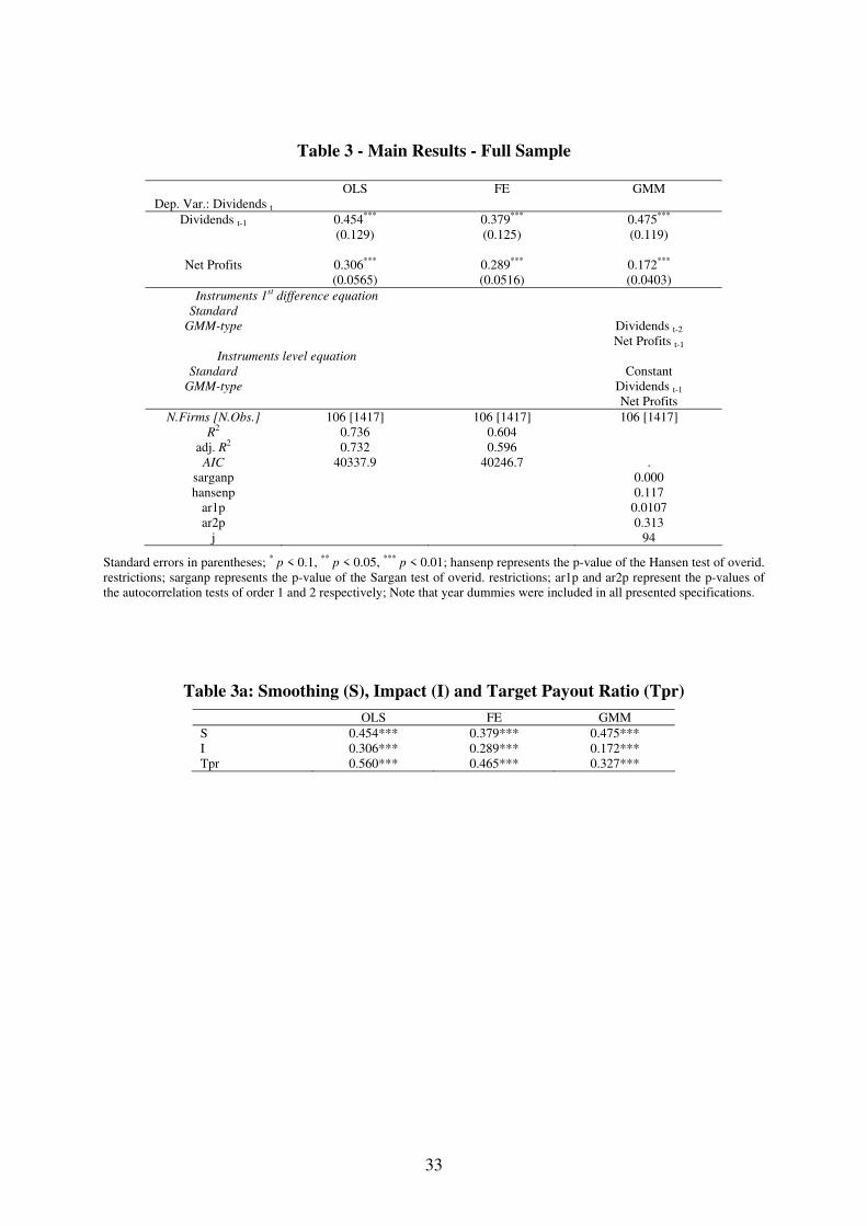
33

Table 3 - Main Results - Full Sample

OLS FE GMM

Dep. Var.: Dividends t

Dividends t-1 0.454*** 0.379*** 0.475*** (0.129) (0.125) (0.119)

Net Profits 0.306*** 0.289*** 0.172*** (0.0565) (0.0516) (0.0403)

Instruments 1st difference equation

Standard GMM-type Dividends t-2

Net Profits t-1 Instruments level equation

Standard Constant GMM-type Dividends t-1

Net Profits

N.Firms [N.Obs.] 106 [1417] 106 [1417] 106 [1417] R

2 0.736 0.604 adj. R2 0.732 0.596

AIC 40337.9 40246.7 . sarganp 0.000 hansenp 0.117

ar1p 0.0107 ar2p 0.313

j 94

Standard errors in parentheses; * p < 0.1, ** p < 0.05, *** p < 0.01; hansenp represents the p-value of the Hansen test of overid. restrictions; sarganp represents the p-value of the Sargan test of overid. restrictions; ar1p and ar2p represent the p-values of the autocorrelation tests of order 1 and 2 respectively; Note that year dummies were included in all presented specifications.

Table 3a: Smoothing (S), Impact (I) and Target Payout Ratio (Tpr)

OLS FE GMM

S 0.454*** 0.379*** 0.475*** I 0.306*** 0.289*** 0.172*** Tpr 0.560*** 0.465*** 0.327***

34

Table 4: First Stage Regressions- Dependent Variable: Inc Reg

FE Logit Logit Sub-sample that switches

from Cost to Inc

Mean_State Control t-1 -0.236*** -3.521*** -3.769*** (0.0823) (0.426) (1.033) Herfindahl Gov. t-1 0.0695 3.285*** 0.375 (0.120) (0.835) (1.188) Checks t-1 0.0332* -0.114 -0.321 (0.0177) (0.121) (0.215) Orientation t-1 -0.0508*** -0.155 -0.528** (0.0192) (0.199) (0.232) Stability t-1 -0.0340 -0.231 -0.222 (0.0596) (0.609) (0.650)

N 380 380 195 R

2 0.657 adj. R2 0.612 AIC 186.3 322.3 141.3

Robust standard errors in parentheses, * p < 0.1, ** p < 0.05, *** p < 0.01

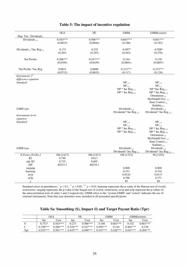
35

Table 5: The impact of incentive regulation

OLS FE GMM GMM(extern)

Dep. Var.: Dividends t

Dividends t-1 0.543*** 0.506*** 0.663*** 0.661*** (0.0815) (0.0844) (0.188) (0.185)

Dividends t-1*Inc Reg t-1 -0.171 -0.232 -0.497* -0.508* (0.201) (0.193) (0.263) (0.276)

Net Profits 0.266*** 0.247*** 0.144 0.130 (0.0395) (0.0439) (0.0891) (0.0897)

Net Profits *Inc Reg 0.0831 0.0690 0.312*** 0.333*** (0.0715) (0.0655) (0.117) (0.128)

Instruments 1st

difference equation

Standard NP t-1 NP t-2

NP * Inc Reg t-1 NP * Inc Reg t-2

NP t-1 NP t-2

NP *Inc Reg t-1 NP * Inc Reg t-2

Orientation t-1 Herfindahl Gov. t-1

State Control t-1

Stability t-1 GMM-type Dividends t-2

Dividends* Inc Reg t-2 Dividends t-2

Dividends* Inc Reg t-2 Instruments level

equation

Standard NP t-1 NP t-2

NP * Inc Reg t-1 NP * Inc Reg t-2

NP t-1 NP t-2

NP * Inc Reg t-1 NP * Inc Reg t-2

Orientation t-1 Herfindahl Gov. t-1

State Control t-1

Stability t-1 GMM-type Dividends t-1

Dividends* Inc Reg t-1 Dividends t-1

Dividends* Inc Reg t-1

N.Firms [N.Obs.] 106 [1417] 106 [1417] 106 [1323] 96 [1103] R2 0.740 0.613

adj. R2 0.735 0.605 AIC 40323.3 40218.1 . .

sarganp 0.000 0.000 hansenp 0.151 0.316

ar1p 0.0124 0.0117 ar2p 0.390 0.371

j 85 89

Standard errors in parentheses; * p < 0.1, ** p < 0.05, *** p < 0.01; hansenp represents the p-value of the Hansen test of overid. restrictions; sarganp represents the p-value of the Sargan test of overid. restrictions; ar1p and ar2p represent the p-values of the autocorrelation tests of order 1 and 2 respectively; GMM refers to the “system GMM” and “extern” indicates the use of external instruments; Note that year dummies were included in all presented specifications.

Table 5a: Smoothing (S), Impact (I) and Target Payout Ratio (Tpr)

OLS FE GMM GMM(extern)

Inc Cost Inc Cost Inc Cost Inc Cost

S 0.372* 0.543*** 0.273 0.506*** 0.166 0.663*** 0.152 0.661*** I 0.349*** 0.266*** 0.316*** 0.247*** 0.456*** 0.144 0.464*** 0.130 Tpr 0.555*** 0.581*** 0.435*** 0.499*** 0.547*** 0.428*** 0.547*** 0.384***

36

Table 6: Profitability and dividend behaviour across regulation and control

Cost Incentive State Private State Private

Profitability

0.035 ~ 0.034 0.043 < *** 0.064 Net Profits/ Total Assets

(0.037) (0.046) (0.059) (0.058) 0.086 > *** 0.078 0.085 < *** 0.102 Cash Flows/ Total Assets

(0.042) (0.050) (0.062) (0.060) 0.101 ~ 0.101 0.105 < *** 0.170 Net Profits/ Equity

(0.089) (0.097) (0.084) (0.157) 0.116 ~ 0.113 0.116 < *** 0.142 Ebitda/ Total Assets

(0.054) (0.055) (0.064) (0.071)

Dividends

0.017 < *** 0.022 0.028 ~ 0.033 Dividends/ Total Assets (0.020) (0.022) (0.032) (0.043) 0.526 < *** 0.618 0.619 > *** 0.481 Dividends/ Net Profits

(0.397) (0.401) (0.528) (0.489) 0.199 < *** 0.263 0.301 ~ 0.278 Dividends/ Cash Flows

(0.193) (0.188) (0.226) (0.238)

17.219 > * 16.145 21.951 > ** 20.529 Price Volatility

(6.329) (6.996) (5.570) (4.791)

* p < 0.1, ** p < 0.05, *** p < 0.01, Significance is reported according to mean difference tests on firm-year observations, Standard deviation in parentheses

37

Table 7: The impact of regulation and control

Dep. Var.: Dividends t OLS FE GMM GMM(extern) GMM(few_inst)

Dividends t-1 0.585*** 0.557*** 0.388*** 0.363*** 0.495** (0.0455) (0.121) (0.0766) (0.0728) (0.208) Div t-1*Inc t-1 * State t-1 0.163** 0.126 0.253** 0.288*** 0.259 (0.0659) (0.145) (0.118) (0.112) (0.272) Divt-1*Inc t-1 * Priv t-1 -0.453*** -0.498*** -0.336*** -0.306** -0.389** (0.0585) (0.140) (0.130) (0.127) (0.178) Divt-1*RoRt-1*Privt-1 -0.0598 -0.103 0.0667 0.0915 0.138 (0.0628) (0.201) (0.166) (0.171) (0.204) Net Profits 0.241*** 0.215*** 0.304*** 0.326*** 0.254** (0.0268) (0.0459) (0.0441) (0.0431) (0.126) Net Profits *Inc * State -0.0503 -0.0597 -0.0424 -0.0665 -0.0256 (0.0449) (0.0621) (0.0658) (0.0648) (0.212) Net Profits *Inc * Priv 0.153*** 0.120 0.121 0.0979 0.112 (0.0349) (0.0950) (0.0932) (0.0922) (0.148) Net Profits* RoR* Priv -0.0158 -0.0319 -0.0576 -0.0743 -0.0301 (0.0343) (0.0724) (0.0790) (0.0779) (0.119)

Instruments 1st diff. equation

Standard NPt-2

NPt-2 *Inc t-2 * State t-2 NPt-2 *Inc t-2 * Priv t-2 NPt-2*RoR t-2 *Privt-2

NP t-2

NP t-2*Inc t-2 * State t-2 NP t-2*Inc t-2 * Priv.t-2

NP t-2 * RoR t-2 * Privt-2

Orientation t-1 Herfindahl Gov. t-1

Stability t-1

Orientation t-1 Herfindahl Gov. t-1

Stability t-1

NP t-2 *Inc t-2 * State t-2 NP t-2 *Inc t-2 *Privt-2

NP t-2 * RoRt-2 * Privt-2

Div t-2*Inc t-2 * State t-2

Divt-2*Inc t-2 * Priv t-2

Div t-2* RoR t-2 * Privt-2

GMM-type Divt-2

Div t-2*Inc t-2 *Statet-2

Div t-2*Inc t-2 * Privt-2

Div t-2*RoRt-2 *Privt-2

Divt-2

Div t-2*Inc t-2 * State t-2

Div t-2*Inc t-2 * Priv t-2

Divt-2*RoR t-2 *Privt-2

NP t-2

Divt-3

Instruments level equation Standard NP t-2

NPt-2*Inc t-2 *State t-2 NP t-2*Inc t-2 * Priv t-2 NP t-2*RoRt-2* Privt-2

NP t-2

NP t-2 *Inc t-2 * State t-2 NP t-2 *Inc t-2 * Privt-2

NP t-2 * Cost t-2 * Privt-2

Orientation t-1 Herfindahl Gov. t-1

Stability t-1

Orientation t-1 Herfindahl Gov. t-1

Stability t-1

NP t-2 *Inc t-2 * State t-2 NP t-2 *Inc t-2 * Privt-2

NP t-2 * Cost t-2 * Private t-2

Div t-2*Inc t-2 * State t-2

Divt-2*Inc t-2 * Priv t-2

Div t-2RoR t-2 * Privt-2 GMM-type Divt-1

Div t-1*Inc t-1* State t-1

Div t-1*Inc t-1 *Priv t-2

Divt-1* RoRt-1 *Prit-1

Div t-1

Div t-1*Inc t-1* State t-1

Div t-1*Inc t-1 * Private t-2

Divs t-1* Cost t-1 * Priv t-1

Net Profits t-1

Dividends t-2

N.Firms [N.Obs.] 106 [1358] 106 [1358] 106 [1263] 96 [1095] 96 [1074] R

2 0.760 0.597 adj. R2 0.754 0.588 AIC 38483.8 38386.8 . . . Sarganp 0.000 0.000 0.000 Hansenp 0.999 1.000 0.394 ar1p 0.0435 0.0389 0.0166 ar2p 0.226 0.125 0.0580 J 159 162 99

Standard errors in parentheses; * p < 0.1, ** p < 0.05, *** p < 0.01; hansenp represents the p-value of the Hansen test of overid.

38

restrictions; sarganp represents the p-value of the Sargan test of overid. restrictions; ar1p and ar2p represent the p-values of the autocorrelation tests of order 1 and 2 respectively; GMM refers to the “system GMM”, “extern” indicates the use of external instruments and “few_inst” the use of fewer instruments; “Dividends*Inc*State” refers to the interaction term between Dividends, a dummy indicating that Inc Reg is equal 1 and a dummy indicating that State Control is equal 1; “Dividends*Inc*Private” refers to the interaction term between Dividends, a dummy indicating that Inc Reg is equal 1 and a dummy indicating that State Control is equal 0; “Dividends* Cost *Private” refers to the interaction term between Dividends, a dummy indicating that Inc Reg is equal 0 and a dummy indicating that State Control is equal 0; “Net Profits*Inc*State” refers to the interaction term between Net Profits, a dummy indicating that Inc Reg is equal 1 and a dummy indicating that State Control is equal 1; “Net Profits*Inc*Private” refers to the interaction term between Net Profits, a dummy indicating that Inc Reg is equal 1 and a dummy indicating that State Control is equal 0; “Net Profits* Cost *Private” refers to the interaction term between Net Profits, a dummy indicating that Inc Reg is equal 0 and a dummy indicating that State Control is equal 0; Note that year dummies were included in all presented specifications.

Table 7a: Smoothing (S), Impact (I) and Target Payout Ratio (Tpr)

GMM GMM(extern)

State Private State Private

Inc Cost Inc Cost Inc Cost Inc Cost

S 0.642*** 0.388*** 0.0524 0.455*** 0.651*** 0.363*** 0.0571 0.455*** I 0.261*** 0.304*** 0.425*** 0.246*** 0.260*** 0.326*** 0.424*** 0.252*** Tpr 0.729*** 0.496*** 0.448*** 0.452*** 0.745*** 0.512*** 0.450*** 0.462***

GMM(few_inst)

State Private

Inc Cost Inc Cost

S 0.754*** 0.495** 0.106 0.633*** I 0.229** 0.254** 0.366** 0.224*** Tpr 0.930*** 0.504*** 0.410*** 0.612***

39

Appendix

Table A1: - Panel Structure

Available Observations

Number of Firms % Cumm. %

6 4 3.77 3.77 7 12 11.32 15.09 8 6 5.66 20.75 9 7 6.60 27.36 10 5 4.72 32.08 11 12 11.32 43.40 12 3 2.83 46.23 13 4 3.77 50.00 14 3 2.83 52.83 15 11 10.38 63.21 16 4 3.77 66.98 17 2 1.89 68.87 18 2 1.89 70.75 19 2 1.89 72.64 20 5 4.72 77.36 21 3 2.83 80.19 22 2 1.89 82.08 23 5 4.72 86.79 24 3 2.83 89.62 25 11 10.38 100.00

N 106

Table A2: Dividend Payout Ratios (Descriptive Statistics for Nations)

Nation Firms Observations Mean Median Std. Deviation

Austria 4 79 54.72% 38.95% 39.47%

Belgium 4 56 67.82% 74.68% 32.45%

Czech Republic 12 107 34.05% 24.68% 42.97%

Denmark 2 25 38.52% 34.26% 28.70%

Finland 3 50 58.62% 40.22% 55.10%

France 5 100 33.05% 30.65% 35.34%

Germany 22 305 67.10% 63.96% 37.13%

Greece 1 10 44.60% 29.22% 47.80%

Hungary 3 28 61.58% 80.08% 61.47%

Italy 9 112 63.51% 57.28% 60.73%

Luxembourg 1 20 62.02% 67.51% 15.39%

Norway 3 49 33.61% 24.12% 39.00%

Portugal 2 22 70.00% 67.58% 25.99%

Spain 8 137 59.92% 56.64% 31.91%

Sweden 3 35 55.51% 43.85% 32.05%

Switzerland 10 188 58.96% 52.33% 38.56%

UK 14 159 43.79% 32.62% 50.28%

Total 106 1,482 54.86% 49.63% 43.35%

Note: Presented data refer to the variable Dividend Payout Ratio.

40

Table A3 - First Stage Analysis: Pairwise correlations

Reg Inc Mean_State

Control Herfindahl

Gov. Checks Orientation Stability

Reg Inc 1

Mean_State Control -0.395*** 1

Herfindahl Gov. 0.172*** 0.167*** 1

Checks -0.061 -0.162*** -0.386*** 1

Orientation -0.071 0.176*** 0.307*** -0.188*** 1

Stability -0.012 0.043 0.092* -0.029 0.002 1

41

Cash flow results

Table A4: Main Results - Full Sample Cash Flows

Dep. Var.: Dividends t OLS FE GMM

Dividends t-1 0.507*** 0.316** 0.395*** (0.141) (0.134) (0.132) Cash Flows 0.140*** 0.236*** 0.117*** (0.0439) (0.0427) (0.0260)

Instruments 1st difference equation

Standard GMM-type Dividends t-2

Cash Flows t-1 Instruments level equation

Standard Constant GMM-type Dividends t-1

Cash Flows

N.Firms [N.Obs.] 106 [1413] 106 [1413] 106 [1413] R

2 0.728 0.626 adj. R2 0.723 0.619 AIC 40270.9 40055.3 . sarganp 0.000 hansenp 0.0852 ar1p 0.0128 ar2p 0.342 j 94

Standard errors in parentheses; * p < 0.1, ** p < 0.05, *** p < 0.01; hansenp represents the p-value of the Hansen test of overid. restrictions; sarganp represents the p-value of the Sargan test of overid. restrictions; ar1p and ar2p represent the p-values of the autocorrelation tests of order 1 and 2 respectively; Note that year dummies were included in all presented specifications.

Table A4a: Smoothing (S), Impact (I) and Tpr - Cash Flows

OLS FE GMM

S 0.507*** 0.316** 0.395*** I 0.140*** 0.236*** 0.117*** Tpr 0.283*** 0.346*** 0.193***

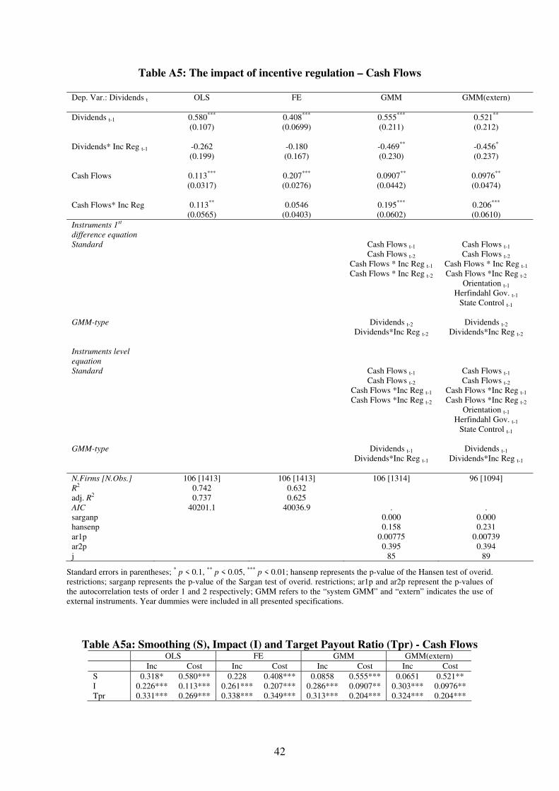
42

Table A5: The impact of incentive regulation – Cash Flows

Dep. Var.: Dividends t OLS FE GMM GMM(extern)

Dividends t-1 0.580*** 0.408*** 0.555*** 0.521** (0.107) (0.0699) (0.211) (0.212) Dividends* Inc Reg t-1 -0.262 -0.180 -0.469** -0.456* (0.199) (0.167) (0.230) (0.237) Cash Flows 0.113*** 0.207*** 0.0907** 0.0976** (0.0317) (0.0276) (0.0442) (0.0474) Cash Flows* Inc Reg 0.113** 0.0546 0.195*** 0.206*** (0.0565) (0.0403) (0.0602) (0.0610)

Instruments 1st

difference equation

Standard Cash Flows t-1

Cash Flows t-2

Cash Flows * Inc Reg t-1

Cash Flows * Inc Reg t-2

Cash Flows t-1

Cash Flows t-2

Cash Flows * Inc Reg t-1 Cash Flows *Inc Reg t-2

Orientation t-1 Herfindahl Gov. t-1

State Control t-1

GMM-type Dividends t-2 Dividends*Inc Reg t-2

Dividends t-2 Dividends*Inc Reg t-2

Instruments level

equation

Standard Cash Flows t-1

Cash Flows t-2

Cash Flows *Inc Reg t-1

Cash Flows *Inc Reg t-2

Cash Flows t-1

Cash Flows t-2

Cash Flows *Inc Reg t-1 Cash Flows *Inc Reg t-2

Orientation t-1 Herfindahl Gov. t-1

State Control t-1

GMM-type Dividends t-1 Dividends*Inc Reg t-1

Dividends t-1 Dividends*Inc Reg t-1

N.Firms [N.Obs.] 106 [1413] 106 [1413] 106 [1314] 96 [1094] R

2 0.742 0.632 adj. R2 0.737 0.625 AIC 40201.1 40036.9 . . sarganp 0.000 0.000 hansenp 0.158 0.231 ar1p 0.00775 0.00739 ar2p 0.395 0.394 j 85 89

Standard errors in parentheses; * p < 0.1, ** p < 0.05, *** p < 0.01; hansenp represents the p-value of the Hansen test of overid. restrictions; sarganp represents the p-value of the Sargan test of overid. restrictions; ar1p and ar2p represent the p-values of the autocorrelation tests of order 1 and 2 respectively; GMM refers to the “system GMM” and “extern” indicates the use of external instruments. Year dummies were included in all presented specifications.

Table A5a: Smoothing (S), Impact (I) and Target Payout Ratio (Tpr) - Cash Flows OLS FE GMM GMM(extern)

Inc Cost Inc Cost Inc Cost Inc Cost

S 0.318* 0.580*** 0.228 0.408*** 0.0858 0.555*** 0.0651 0.521** I 0.226*** 0.113*** 0.261*** 0.207*** 0.286*** 0.0907** 0.303*** 0.0976** Tpr 0.331*** 0.269*** 0.338*** 0.349*** 0.313*** 0.204*** 0.324*** 0.204***

43

Table A6: The impact of regulation and control - Cash Flows OLS FE GMM GMM(extern) GMM(few_inst) Dep. Var.: Dividends t

Dividends t-1 0.664*** 0.505*** 0.348*** 0.343*** 0.541*** (0.0409) (0.0921) (0.0918) (0.0868) (0.143) Dividends t-1*Inc t-1 * State t-1 0.0419 0.146 0.199* 0.234* -0.0406 (0.0613) (0.113) (0.119) (0.123) (0.280) Dividends t-1*Inc t-1 * Private t-1 -0.617*** -0.511*** -0.393*** -0.413*** -0.623*** (0.0549) (0.108) (0.132) (0.120) (0.209) Dividends t-1* Cost t-1 * Private t-1 -0.363*** -0.197 -0.175 -0.238 -0.305 (0.0621) (0.172) (0.169) (0.162) (0.247) Cash Flows 0.0699*** 0.146*** 0.106*** 0.106*** 0.0708** (0.00882) (0.0213) (0.0204) (0.0194) (0.0277) Cash Flows *Inc * State 0.0495** -0.00598 0.0781*** 0.0649** 0.149 (0.0208) (0.0243) (0.0263) (0.0275) (0.141) Cash Flows *Inc * Private 0.222*** 0.142*** 0.222*** 0.236*** 0.271*** (0.0171) (0.0528) (0.0525) (0.0456) (0.0884) Cash Flows * Cost * Private 0.134*** 0.0836* 0.137*** 0.159*** 0.184*** (0.0166) (0.0497) (0.0394) (0.0342) (0.0650)

Instruments 1st difference equation

Standard CF t-2

CFt-2*Inc t-2* State t-2 CFt-2*Inc t-2 * Privt-2 CF t-2*RoR t-2*Privt-2

CF t-2

CF t-2 *Inc t-2 * State t-2 CFt-2 *Inc t-2 * Priv t-2 CFt-2*Cost t-2 *Priv t-2

Orientation t-1 Herfindahl Gov.t-1

Stability t-1

Orientation t-1 Herfindahl Gov. t-1

Stability t-1

CFt-2*Inc t-2*Statet-2 CFt-2*Inc t-2 * Privt-2 CFt-2*Cost t-2*Privt-2

Div t-2*Inc t-2 *Statet-2

Divt-2*Inc t-2 * Privt-2

Divt-2*Cost t-2 * Privt-2

GMM-type Divt-2

Div t-2*Inct-2 *State -2

Divt-2*Inc t-2 * Privt-2

Divt-2* Cost t-2 * Privt-2

Divt-2

Divt-2*Inct-2* State t-2

Divt-2*Inc t-2 * Privt-2

Divt-2*Cost t-2 * Privt-2

CFlt-2

Divt-3

Instruments level equation Standard CF t-2

CF t-2*Inc t-2*State t-2 CF t-2 *Inc t-2*Priv t-2 CF t-2*RoRt-2*Priv t-2

CF t-2

CF t-2 *Inc t-2 * State t-2 CF t-2 *Inc t-2 * Privt-2

CF t-2 *RoR t-2 *Priv t-2

Orientation t-1 Herfindahl Govt-1

Stability t-1

Orientation t-1 Herfindahl Gov. t-1

Stability t-1

CF t-2 *Inc t-2 * State t-2 CF t-2*Inc t-2 * Private t-2

CF t-2*Rort-2 * Privt-2

Divt-2*Inc t-2 *State t-2

Div t-2*Inc t-2 * Privt-2

Divt-2*Rort-2 *Privt-2 GMM-type Div t-1

Div t-1*Inct-1*State t-1

Divt-1*Inc t-1 * Privt-2

Div t-1*RoRt-1 *Privt-1

Divt-1

Divt-1*Inct-1*State t-1

Divt-1*Inc t-1 * Privt-2

Divt-1*RoRt-1 * Privt-1

CF t-1

Divt-2

N.Firms [N.Obs.] 106 [1354] 106 [1354] 106 [1255] 96 [1087] 96 [1068] R

2 0.774 0.618 adj. R2 0.768 0.609 AIC 38295.7 38206.1 . . . sarganp 0.000 0.000 0.000 hansenp 0.997 1.000 0.195 ar1p 0.0396 0.0520 0.0297 ar2p 0.146 0.180 0.300 J 159 162 99

Standard errors in parentheses; * p < 0.1, ** p < 0.05, *** p < 0.01; hansenp represents the p-value of the Hansen test of overid. restrictions; sarganp represents the p-value of the Sargan test of overid. restrictions; ar1p and ar2p represent the p-values of

44

the autocorrelation tests of order 1 and 2 respectively; GMM refers to the “system GMM”, “extern” indicates the use of external instruments and “few_inst” the use of fewer instruments; “Dividends*Inc*State” refers to the interaction term between Dividends, a dummy indicating that Inc Reg is equal 1 and a dummy indicating that State Control is equal 1; “Dividends*Inc*Private” refers to the interaction term between Dividends, a dummy indicating that Inc Reg is equal 1 and a dummy indicating that State Control is equal 0; “Dividends* Cost *Private” refers to the interaction term between Dividends, a dummy indicating that Inc Reg is equal 0 and a dummy indicating that State Control is equal 0; “Cash Flows *Inc*State” refers to the interaction term between Cash Flows, a dummy indicating that Inc Reg is equal 1 and a dummy indicating that State Control is equal 1; “Cash Flows *Inc*Private” refers to the interaction term between Cash Flows, a dummy indicating that Inc Reg is equal 1 and a dummy indicating that State Control is equal 0; “Cash Flows * Cost *Private” refers to the interaction term between Cash Flows, a dummy indicating that Inc Reg is equal 0 and a dummy indicating that State Control is equal 0; Note that year dummies were included in all presented specifications.

Table A6a: Smoothing (S), Impact (I) and Target Payout Ratio (Tpr) - Cash Flows

GMM GMM(extern)

State Private State Private

Inc Cost Inc Cost Inc Cost Inc Cost

S 0.547*** 0.348*** - 0.172 0.577*** 0.343*** - 0.104 I 0.184*** 0.106*** 0.327*** 0.243*** 0.171*** 0.106*** 0.342*** 0.265***

Tpr 0.405*** 0.162*** 0.313*** 0.294*** 0.404*** 0.161*** 0.320*** 0.296***

GMM(few_inst)

State Private

Inc Cost Inc Cost

S 0.500* 0.541*** - 0.236 I 0.220* 0.0708** 0.342*** 0.255***

Tpr 0.441*** 0.154*** 0.316*** 0.333***

45

Table A7: Incentive vs Cost-Based Regulation - Analysis by sub-sampling

Dep. Var.: Dividends t OLS FE GMM Inc Cost Inc Cost Inc Cost

Dividends t-1 0.303 0.644*** 0.0558 0.610*** 0.446* 0.761*** (0.181) (0.0967) (0.101) (0.0917) (0.268) (0.123) Net Profits t-3 0.403*** 0.234*** 0.285*** 0.233*** 0.377*** 0.115* (0.0657) (0.0435) (0.0458) (0.0523) (0.135) (0.0592)

Instruments 1st difference equation

Standard GMM-type Dividends t-3

Net Profits t-3 Dividends t-3 Net Profits t-2

Instruments level equation Standard Constant Constant GMM-type Dividends t-2

Net Profits t-2 Dividends t-2 Net Profits t-2

N.Firms [N. Obs.] 65 [443] 85 [974] 65 [443] 85 [974] 65 [443] 85 [974] R

2 0.678 0.819 0.304 0.756 adj. R2 0.661 0.815 0.267 0.749 AIC 12933.0 27025.6 12831.9 26979.5 . . sarganp 0.000 0.000 hansenp 0.813 0.480 ar1p 0.0252 0.160 ar2p 0.246 0.804 j 72 93

Standard errors in parentheses; * p < 0.1, ** p < 0.05, *** p < 0.01; hansenp represents the p-value of the Hansen test of overid. restrictions; sarganp represents the p-value of the Sargan test of overid. restrictions; ar1p and ar2p represent the p-values of the autocorrelation tests of order 1 and 2 respectively; “Inc” refers to incentive regulation and “RoR” to RoR regulation; Note that year dummies were included in all presented specifications.

Table A7a: Smoothing (S), Impact (I) and Target Payout (Tpr) using Net Profits

OLS FE GMM

Inc Cost Inc Cost Inc Cost

S 0.303 0.644*** 0.0558 0.610*** 0.446* 0.761*** I 0.403*** 0.234*** 0.285*** 0.233*** 0.377*** 0.115* Tpr 0.578*** 0.656*** 0.302*** 0.599*** 0.681*** 0.480*

46

Table A8: Incentive vs Cost-Based Regulation - Analysis by sub-sampling - Cash Flows

Dep. Var.: Dividends t OLS FE GMM

Inc Cost Inc Cost Inc Cost

Dividends t-1 0.190 0.732*** 0.0739 0.489*** 0.278 0.667*** (0.170) (0.0908) (0.125) (0.0967) (0.254) (0.153) Cash Flows 0.286*** 0.0867*** 0.217*** 0.200*** 0.284*** 0.0840*** (0.0489) (0.0241) (0.0556) (0.0326) (0.0845) (0.0304)

Instruments 1st difference equation Standard GMM-type Dividends t-3

Cash Flows t-3 Dividends t-3 Cash Flows t-2

Instruments level equation Standard Constant Constant GMM-type Dividends t-2

Cash Flows t-2 Dividends t-2 Cash Flows t-2

N 65 [443] 85 [970] 65 [443] 85 [970] 65 [443] 85 [970] R

2 0.709 0.804 0.300 0.772 adj. R2 0.694 0.799 0.263 0.766 AIC 12887.9 26996.7 12834.3 26806.9 . . Sarganp 0.00160 1.97e-34 Hansenp 0.850 0.512 ar1p 0.0281 0.162 ar2p 0.306 0.971 J 72 93

Standard errors in parentheses; * p < 0.1, ** p < 0.05, *** p < 0.01; hansenp represents the p-value of the Hansen test of overid. restrictions; sarganp represents the p-value of the Sargan test of overid. restrictions; ar1p and ar2p represent the p-values of the autocorrelation tests of order 1 and 2 respectively; “Inc” refers to incentive regulation and “RoR” to RoR regulation; Note that year dummies were included in all presented specifications.

Table A8a: Smoothing (S), Impact (I) and Target Payout Ratio (Tpr)

OLS FE GMM

Inc Cost Inc Cost Inc Cost

S 0.190 0.732*** 0.0739 0.489*** 0.278 0.667*** I 0.286*** 0.0867*** 0.217*** 0.200*** 0.284*** 0.0840*** Tpr 0.353*** 0.324*** 0.235*** 0.391*** 0.393*** 0.252***