dividend discount approach to equity derivatives · pdf fileintroduction a ne dividends...

IntroductionAffine dividends

Homogenous dividend dynamicsConclusion

Dividend Discount Approach to Equity Derivatives Modelling

Oliver BrockhausMathFinance AG

[email protected]

Cass Business SchoolLondon, 3 December 2014

[email protected] Dividend Discount Approach to Equity Derivatives Modelling 1 / 32

mailto:[email protected]



Agenda

1 IntroductionResearchEquity dynamicsDividend discount modelsCalibration

2 Affine dividendsBos-VandermarkAffine stock processAffine dividend dynamics

3 Homogenous dividend dynamicsIndicator functionKorn-RogersPiecewise linearExponential

4 ConclusionSummaryReferences




ResearchEquity dynamicsDividend discount modelsCalibration

Research

There are various directions of research on the topic of dividends:

Empirical properties, forecasting:van Binsbergen et al. [vBBK10]

Dividends within equity dynamics:Bos-Vandermark [BV02] (closed form formula with discrete dividends)Overhaus et al. [OFK+02] and [OBB+07] (affine model)Vellekoop, Nieuwenhuis [VN06] (model survey)

Dividend discount models:Korn-Rogers [KR05] (dividend announcement)Bernhart, Mai [BM12] (general framework)

Dividend derivatives modelling:Tunaru [Tun14] (uncertain timing, cum dividend process)Buhler et al. [BDS10] (discrete dividends with stochastic yield)





Equity dynamics

When modelling equity dynamics there are two popular ways of incorporatingdividends:

Continuous dividend payment stream, proportional to spot level S , namelycontinuous dividend yield q:

dSt

St= (rt − qt)dt + σtdWt

Discrete dividends with known future ex-dividend dates0 < t1 < t2 < . . . , namely

D iti = fi (Sti−)

with deterministic fi . In practice one often assumesdeterministic payments in the near future: fi = ciproportional dividends for the distant future: fi (Sti−) = ciSti−Positivity of S is preserved if fi is capped at Sti− or fi (x) ≤ x .





Dividend discount models

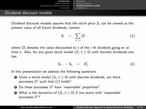
Dividend discount models assume that the stock price St can be viewed as thepresent value of all future dividends, namely

St =∑ti>t

D it (1)

where D it denotes the value discounted to t of the i-th dividend going ex at

time ti . Also, for any given stock model (St , t ≥ 0) with discrete dividends onehas

Sti− − Sti = D iti (2)

In this presentation we address the following questions:

1 Given a stock model (St , t ≥ 0) with discrete dividends, are thereprocesses D i such that (1) holds?

2 Do these processes D i have ‘reasonable’ properties?

3 What is the dynamics of (St , t ≥ 0) if one starts with ‘reasonable’processes D i?





Calibration

Let Ft and Pt denote equity forward and discount factor, respectively. One hasthe calibration condition

PtFt = S0 −∑ti≤t

D i0 =

∑ti>t

D i0 (3)

If a stock does not pay dividends then one may assume a single dividendpayment at infinity with value Dt = St at time t. Otherwise one can assume D i

0

to be known for all i up to some index k.With exponential growth thereafter, namely

D i0 = Dk

0 e−q∆(i−k) and ti = tk + ∆(i − k)

for all i ≥ k and some time increment ∆ one computes

q∆ = logS0 −

∑i<k D

i0

S0 −∑

i≤k Di0

= logPtk−1Ftk−1

PtkFtk

from (1) or (3) with t = 0. Growth parameter q can be interpreted as longterm dividend yield.




Bos-VandermarkAffine stock processAffine dividend dynamics

Bos-Vandermark

In a famous article Bos and Vandermark [BV02] present a variant of the BlackScholes formula, namely

CBV (K , t) = PtBlack(P−1t (S0 − X n

t ),K + P−1t X f

t , σ2t)

(4)

with deterministic functions

X nt =

∑ti≤t

(t − ti )+

tD i

0 X ft =

∑ti≤t

ti ∧ t

tD i

0

and volatility σ.

This formula is a good approximation for a European option price withdeterministic dividend drops and volatility σ in between. Additionally, theformula is continuous both as valuation date moves across a dividend andmaturity moves across a dividend. The model as defined in their paper dependson the maturity t of the European option.





Bos-Vandermark

We now fix t independently of the product, namely

X n,Tt =

∑ti≤t

(T − ti )+

TD i

0 X f ,Tt =

∑ti≤t

ti ∧ T

TD i

0

Inserting X n,Tt ,X f ,T

t rather than X nt ,X

ft into formula (4) implies a stock

process S given as

PtSt = (S0 − X n,Tt )Mt − X f ,T

t

where M is a geometric Brownian motion with mean 1 and volatility σ. Thisgives rise to affine dividends, namely

Sti− − Sti = P−1ti D i

0

((T − ti )

+

TMti +

ti ∧ T

T

)= P−1

ti D i0

((T − ti )

+

T

PtiSti− + X f ,Tti−

S0 − X n,Tti−

+ti ∧ T

T

)= αi + βiSti−

Note that αi ↘ 0 for ti ↘ 0 and βi ↘ 0 for ti ↗ T .





Affine stock process

It is now standard to model dividends as affine functions of the spot at theex-date

D iti = αi + βiSti− (5)

with for example βi = 0 for ti < 1y and αi = 0 if ti ≥ 5y .

This is equivalent to the stock process being an affine function in the sense that

St = (Ft − Ct)Mt + Ct (6)

holds for some martingale M and a deterministic function C .

This approach dates back to [BFF+00] p7f. More recent references includeOverhaus et al. [OFK+02] p116ff as well as [OBB+07] p6ff.






More formally, one has (compare Overhaus et al. [OBB+07] p7):

Proposition (affine stock model): Assume a stock process S with jumps dueto dividends only. The following two statements are equivalent:

1 The stock process S is positive and pays positive affine dividends (5)satisfying

αi = 0 for all i ≥ n for some nβi ∈ [0, 1) for all i

Ptiαi ≥ −βi∑

j≥i Ptjαj

∏jk=i (1− βk)−1 for all i

2 The stock process S is an affine function (6) of a positive continuousmartingale M with M0 = 1 where C satisfies

Ct = 0 for all t ≥ T for some T∆Ft ≤ ∆Ct ≤ 0 for all t

dCt = rCt for all t /∈ {t1, t2, . . . }

with notation ∆ft ≡ ft − ft− for a given cadlag function f .






(2)⇒ (1): Substituting (6) into the dividend drop Sti− − Sti yields

Sti− − Sti = (−∆Fti + ∆Cti )Mti− −∆Cti

= (−∆Fti + ∆Cti )Sti− − Cti−

Fti− − Cti−−∆Cti ≥ 0

and hence

αi =Cti−∆Fti − Fti−∆Cti

Fti− − Cti−βi = −∆(Fti − Cti )

Fti− − Cti−

One computes

αi + βiCti− = −∆Cti = Cti− −Pti+1

Pti

Cti+1−

and hence

PtiCti− =Ptiαi

1− βi+

Pti+1Cti+1−

1− βi= . . . =

∑j≥i

Ptjαj

j∏k=i

(1− βk)−1

The properties of C imply the required properties of αi and βi for all i as wellas positivity of S .






(1)⇒ (2): Both C and M can be constructed by induction on [ti−1, ti ) if givenon t ≥ ti such that (6) holds:

For t ≥ tn define Ct = 0 as well as Mt through St = FtMt .If C is defined for t ≥ ti set

−∆Cti = αi + βiCti− =αi + βiCti

1− βi(7)

This defines C and hence M through (6) on t ≥ ti−1, and one has

∆Sti = (∆Fti −∆Cti )Sti− − Cti−

Fti− − Cti−+ ∆Cti = . . . = −βiSti− − αi

where we used

−∆Fti = αi + βiFti− =αi + βiFti

1− βiNote that as seen above (7) yields via induction

PtiCti− =∑j≥i

Ptjαj

j∏k=i

(1− βk)−1

Hence C has the required properties. Continuity of M at ti can also beestablished.





Examples

Special cases include

Proportional dividends: Ct = 0

Deterministic dividends up to some final date T :

PtCt =∑

T≥ti>t

D i0

Without T one has the deterministic case St = Ft due to (3).

Blend model:

PtCt =∑ti>t

(1− τi )D i0 (8)

with some increasing sequence τ in [0, 1].

We have seen above that Bos-Vandermark is a model with affinedividends. Since Ct ≤ 0 the stock process can be negative.





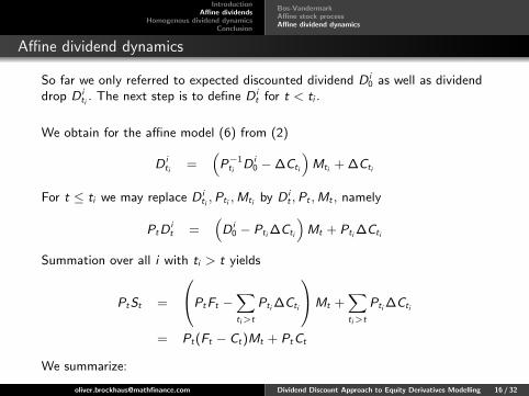
Affine dividend dynamics

So far we only referred to expected discounted dividend D i0 as well as dividend

drop D iti . The next step is to define D i

t for t < ti .

We obtain for the affine model (6) from (2)

D iti =

(P−1ti D i

0 −∆Cti

)Mti + ∆Cti

For t ≤ ti we may replace D iti ,Pti ,Mti by D i

t ,Pt ,Mt , namely

PtDit =

(D i

0 − Pti ∆Cti

)Mt + Pti ∆Cti

Summation over all i with ti > t yields

PtSt =

PtFt −∑ti>t

Pti ∆Cti

Mt +∑ti>t

Pti ∆Cti

= Pt(Ft − Ct)Mt + PtCt

We summarize:





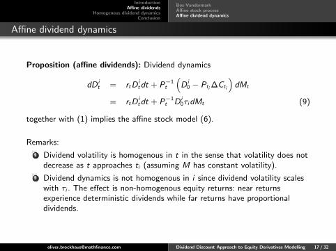
Affine dividend dynamics

Proposition (affine dividends): Dividend dynamics

dD it = rtD

itdt + P−1

t

(D i

0 − Pti ∆Cti

)dMt

= rtDitdt + P−1

t D i0τidMt (9)

together with (1) implies the affine stock model (6).

Remarks:

1 Dividend volatility is homogenous in t in the sense that volatility does notdecrease as t approaches ti (assuming M has constant volatility).

2 Dividend dynamics is not homogenous in i since dividend volatility scaleswith τi . The effect is non-homogenous equity returns: near returnsexperience deterministic dividends while far returns have proportionaldividends.




Indicator functionKorn-RogersPiecewise linearExponential

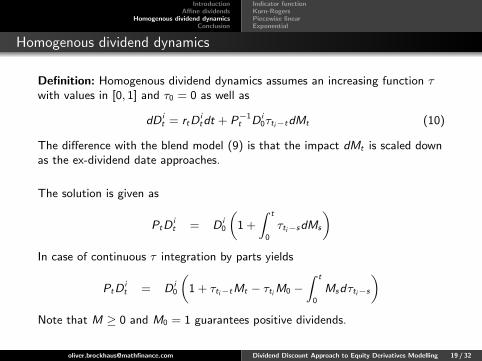
Homogenous dividend dynamics

Definition: Homogenous dividend dynamics assumes an increasing function τwith values in [0, 1] and τ0 = 0 as well as

dD it = rtD

itdt + P−1

t D i0τti−tdMt (10)

The difference with the blend model (9) is that the impact dMt is scaled downas the ex-dividend date approaches.

The solution is given as

PtDit = D i

0

(1 +

∫ t

0

τti−sdMs

)In case of continuous τ integration by parts yields

PtDit = D i

0

(1 + τti−tMt − τtiM0 −

∫ t

0

Msdτti−s

)Note that M ≥ 0 and M0 = 1 guarantees positive dividends.





Homogenous dividend dynamics

Proposition (homogenous dividends): With homogenous dividend dynamicsthe stock process is given as sum of an affine function and an integral of themartingale M. More specifically:

St = Ft + P−1t

(T tt Mt − T t

0 M0 −∫ t

0

MsdT ts

)with T t

s for 0 ≤ s ≤ t defined as

T ts =

∑ti>t

D i0τti−s

Proof: One has

PtSt = Pt

∑ti>t

D it

=∑ti>t

D i0

(1 + τti−tMt − τtiM0 −

∫ t

0

Msdτti−s

)





Examples: indicator function

Dividend announcement at a fixed time interval a before the ex-date isrepresented by the indicator function

τt = 1{t>a}

Assuming M0 = 1 one has

PtDit = D i

0

(1 +

∫ t

0

1{ti−s>a}dMs

)= D i

0Mt∧(ti−a)+

and

St =∑ti>t

D it = P−1

t

∑ti−a>t

D i0Mt +

∑ti>t≥ti−a

D i0M(ti−a)+

(11)





Examples: Korn-Rogers

The situation discussed by Korn and Rogers [KR05] is obtained by furtherspecializing

ti = ih, a = (1− ε)h ≥ 0, Mt = e−µtXt/X0, Pt = e−rt

where X is an exponential Levy process with mean

IE [ Xt ] = X0eµt

as well asD i

0 = λX0Pti−aeµ(ti−a)





Examples: Korn-Rogers

Formula (11) yields

St = λ∑

(i−1+ε)h>t

e(µ−r)((i−1+ε)h−t)Xt

+ λ∑

ih>t≥(i−1+ε)h

er(t−(i−1+ε)h)X(i−1+ε)h

The second sum is either empty if the next dividend after t has not beenannounced yet or has exactly one term.

Note that formula (11) also covers the case of longer announcement periods,namely a > h or ε < 0. In that case the second sum consisting of all dividendsannounced at t may have more than one term.





Examples: piecewise linear

An alternative to the indicator function is the piecewise linear function

τt =t

a∧ 1

where a is the time distance beyond which a given dividend has maximalvolatility. One obtains for t ≥ a

PtSt =

Pa+tFa+t +∑

a+t≥ti>t

D i0ti − t

a

Mt + a−1∑

a+t≥ti>t

D i0

∫ t

(ti−a)+

Msds

For t < a one has to add the term∑a≥ti>t

D i0

(1− ti

a

)representing the announced part of near dividends.





Examples: exponential

With

τt = 1− e−λt

one obtains

T ts = Pt

(Ft − eλsCt

)dT t

s = λPtCteλsds

where Ct is defined through

PtCt =∑ti>t

D i0e−λti

Thus

St = Ct +(Ft − eλtCt

)Mt + λCt

∫ t

0

eλsMsds

The corresponding non-homogenous affine dividend model (6) is

St = Ct + (Ft − Ct)Mt





Examples: exponential

λ = 0.5, σ = 20%, r = 5%, annual dividends d = 10% paid before maturity




SummaryReferences

Conclusion

Affine stock models (including Bos-Vandermark) can be viewed as dividenddiscount models where all dividends are driven by the same martingalefactor. The volatility level of each dividend does not change through time.

Homogenous dividend models behave like bonds in the sense that theirvolatility level decreases through time, reaching zero at the ex-date.

The stock return distribution of homogenous dividend models is morereasonable as one does not shift from affine for near returns toproportional for far returns.

Modelling homogenous dividend models is more involved since the stockprocess is a time average of a postive martingale.




SummaryReferences

Bibliography I

H. Buhler, A. Dhouibi, and D. Sluys.

Stochastic proportional dividends.http://ssrn.com/abstract=1706758, 2010.

O. Brockhaus, M. Farkas, A. Ferraris, D. Long, and M. Overhaus.

Equity Derivatives and Market Risk Models.Risk Books, February 2000.

G. Bernhart and J. Mai.

Consistent modeling of discrete cash dividends.Technical report, Xaia Investment, 2012.

M. Bos and S. Vandermark.

Finessing fixed dividends.Risk, pages 157–158, 2002.

R. Korn and L. C. G. Rogers.

Stocks paying discrete dividends modeling and option pricing.Journal of Derivatives, 13(2):44–48, 2005.

M. Overhaus, A. Bermudez, H. Buhler, A. Ferraris, C. Jordinson, and A. Lamnouar.

Equity Hybrid Derivatives.John Wiley and Sons, 2007.

M. Overhaus, A. Ferraris, T. Knudsen, R. Milward, L. Nguyen-Ngoc, and G. Schindlmayr.

Equity Derivatives: Theory and Applications.John Wiley and Sons, February 2002.


http://ssrn.com/abstract=1706758



SummaryReferences

Bibliography II

R. Tunaru.

Dividend derivatives.ssrn, 2014.

J. van Binsbergen, M. Brandt, and R Koijen.

On the timing and pricing of dividends.Technical report, National Bureau of Economic Research, 2010.

M.H. Vellekoop and M.H. Nieuwenhuis.

Efficient pricing of derivatives on assets with discrete dividends.Applied Mathematical Finance, 13(3):265–284, 2006.


Appendix: stochastic dividend yield

Buhler [BDS10] suggests an Ornstein-Uhlenbeck process y driving dividendyield. The resulting dynamics can be written as

St = FtNtiMt ti ≤ t < ti+1

where N is an adapted process of the form

Nt =S0

Fte−

∑ti≤t di =

S0

Fte−

∑ti≤t Ci+Di+Ei yt = e

−∑

ti≤t Ci+Ei yt

with IE [ MtiNti ] = 1, PtiFti = e−DiPti−1Fti−1 as well as Ei ∈ {1,Di}.

Remark: It is not required that N or NM is a martingale and indeed

IEti−1 [ Nti ] = Nti−1e−Ci IEti−1

[e−Ei yti

]6= Nti−1


Appendix: stochastic dividend yield

The dividend drop D iti satisfies

PtiDiti = −Pti ∆Sti =

(Pti−1Fti−1Nti−1 − PtiFtiNti

)Mti

A consistent dividend dynamics for t ≤ ti can be defined as

PtDit =

(Pti−1Fti−1Nti−1∧t − PtiFtiNti∧t

)Mt

For t ≤ ti−1 this simplifies to

PtDit = D i

0NtMt

One observes

PtSt = Pt

∑ti>t

D it = Pti−1Fti−1Nti−1Mt ti−1 ≤ t < ti

as required. Buhler [BDS10] also discusses affine dividends

D iti = αi + βiSti− = αi +

(1− Nti

Nti−1

)Sti−

Analysis of a version of this model with homogenous dividend dynamics is leftfor future research.


dividend discount approach to equity derivatives · pdf fileintroduction a ne dividends...

Documents