distributions in insurance risk models - uni-sofia.bg...distributions in insurance risk models leda...
TRANSCRIPT

Distributions in Insurance RiskModels
Leda D.Minkova
A Thesis submitted for the degree of Doctor of Science
Faculty of Mathematics and Informatics
Sofia University ”St.Kl.Ohridski”
2012

Contents
1 Introduction 1
1.1 Risk Model . . . . . . . . . . . . . . . . . . . . . . . . . . . . 1
1.2 Counting probability distributions . . . . . . . . . . . . . . . . 3
1.3 Generalized Power Series distributions . . . . . . . . . . . . . 5
1.4 The (a, b) class of discrete distributions . . . . . . . . . . . . . 6
1.5 Zero - inflated distributions . . . . . . . . . . . . . . . . . . . 7
2 I - Generalized Power Series Distributions 9
2.1 Geometric distribution related to Markov chain . . . . . . . . 10
2.1.1 ρ - Type Lack of Memory Property . . . . . . . . . . . 11
2.2 Negative binomial distribution related to a Markov chain . . . 13
2.3 Poisson limiting distribution . . . . . . . . . . . . . . . . . . . 16
2.4 I - parameter Binomial distribution . . . . . . . . . . . . . . . 20
2.5 I - parameter Logarithmic series distribution . . . . . . . . . . 23
2.6 The family of I - parameter GPSD . . . . . . . . . . . . . . . 27
2.6.1 Common representation of the PMFs . . . . . . . . . . 27
2.6.2 Explicit expressions for PMFs . . . . . . . . . . . . . . 28
2.7 The PGF of the family of IGPSDs . . . . . . . . . . . . . . . . 30
2.8 Compound Generalized Power series distributions . . . . . . . 32
2.8.1 Properties of the IGPSDs . . . . . . . . . . . . . . . . 38
2.8.2 A Characterization of the I - Geometric distribution . . 42
2.8.3 Properties of the INBD . . . . . . . . . . . . . . . . . . 47
2.9 Numerical example . . . . . . . . . . . . . . . . . . . . . . . . 49
i

CONTENTS ii
2.9.1 IPo(λ, ρ) - case . . . . . . . . . . . . . . . . . . . . . . 49
2.9.2 INB(π, ρ, r) - case . . . . . . . . . . . . . . . . . . . . 51
2.10 Comments . . . . . . . . . . . . . . . . . . . . . . . . . . . . . 53
3 Probability distributions of order k 55
3.1 Poisson distribution of order k . . . . . . . . . . . . . . . . . . 57
3.2 Polya - Aeppli distribution of order k . . . . . . . . . . . . . . 58
3.3 Comments . . . . . . . . . . . . . . . . . . . . . . . . . . . . . 62
4 Distributions on Markov chain trials 63
4.1 Geometric distribution of order k . . . . . . . . . . . . . . . . 64
4.1.1 The joint PGF of the random vector S . . . . . . . . . 65
4.1.2 Number of successes in SK0. . . . . . . . . . . . . . . . 67
4.1.3 Number of failures . . . . . . . . . . . . . . . . . . . . 68
4.1.4 Number of trials . . . . . . . . . . . . . . . . . . . . . 70
4.1.5 The joint PGF gS,F (t, s) . . . . . . . . . . . . . . . . . 74
4.2 Quotas on runs in a multi-state Markov chain . . . . . . . . . 74
4.2.1 Sooner waiting time problems . . . . . . . . . . . . . . 75
4.2.2 Exact Distribution of the number of successes . . . . . 82
4.2.3 Exact distribution of the number of failures . . . . . . 84
4.2.4 Later waiting time problems . . . . . . . . . . . . . . . 86
4.3 Run and frequency Quotas in a multi-state Markov cnain . . . 87
4.3.1 Run Quota on successes and frequency Quota on failures 88
4.3.2 Run Quota on failures and frequency Quota on successes 94
4.3.3 Comments . . . . . . . . . . . . . . . . . . . . . . . . . 98
5 I - Stochastic processes 100
5.1 The Polya - Aeppli process . . . . . . . . . . . . . . . . . . . . 100
5.1.1 Moments . . . . . . . . . . . . . . . . . . . . . . . . . . 105
5.2 I - Polya process . . . . . . . . . . . . . . . . . . . . . . . . . 105
5.2.1 Properties of the I - Polya process . . . . . . . . . . . . 106
5.2.2 Moments . . . . . . . . . . . . . . . . . . . . . . . . . . 108
5.3 I - Binomial process . . . . . . . . . . . . . . . . . . . . . . . . 109

CONTENTS iii
5.3.1 Properties of the I-Binomial process . . . . . . . . . . . 109
5.3.2 Moments . . . . . . . . . . . . . . . . . . . . . . . . . . 111
5.4 Inflated - parameter modification of the pure birth process . . 112
5.5 Generalized Delaporte distribution. . . . . . . . . . . . . . . . 114
5.6 Stochastic processes of order k . . . . . . . . . . . . . . . . . . 115
5.6.1 Polya - Aeppli process of order k . . . . . . . . . . . . 115
5.7 Comments . . . . . . . . . . . . . . . . . . . . . . . . . . . . . 117
6 Risk Models 118
6.1 The Polya - Aeppli risk model . . . . . . . . . . . . . . . . . . 119
6.1.1 The ordinary case . . . . . . . . . . . . . . . . . . . . . 119
6.1.2 The stationary case . . . . . . . . . . . . . . . . . . . . 123
6.1.3 The Cramer - Lundberg approximation . . . . . . . . . 125
6.1.3.1 The ordinary case . . . . . . . . . . . . . . . 125
6.1.3.2 The stationary case . . . . . . . . . . . . . . . 127
6.1.4 Comparison of ruins . . . . . . . . . . . . . . . . . . . 127
6.1.5 Martingales for the Polya - Aeppli risk model . . . . . 129
6.1.6 Martingale approach to the Polya-Aeppli risk model . . 130
6.1.7 Reinsurance . . . . . . . . . . . . . . . . . . . . . . . . 132
6.2 Compound Birth process . . . . . . . . . . . . . . . . . . . . . 136
6.2.1 Probability generating function . . . . . . . . . . . . . 137
6.2.2 Application to Risk Theory . . . . . . . . . . . . . . . 137
6.2.3 Examples . . . . . . . . . . . . . . . . . . . . . . . . . 140
6.2.4 Polya - Aeppli process . . . . . . . . . . . . . . . . . . 140
6.2.5 I - Polya process . . . . . . . . . . . . . . . . . . . . . 141
6.2.6 I - Binomial process . . . . . . . . . . . . . . . . . . . 141
6.2.7 Exponentially distributed claims . . . . . . . . . . . . . 142
6.3 Comments . . . . . . . . . . . . . . . . . . . . . . . . . . . . . 142
7 Concluding remarks 143

CONTENTS iv
Appendix 145
Gaussian hypergeometric function . . . . . . . . . . . . . . . . 145
Confluent Hypergeometric function . . . . . . . . . . . . . . . 146
Incomplete Gamma functions . . . . . . . . . . . . . . . . . . 146
Bibliography 147

Chapter 1
Introduction
1.1 Risk Model
The foundation of the modern risk theory goes back to the works of Filip
Lundberg and Harald Cramer. In 1903 Filip Lundberg proposed the Poisson
process as a simple process in solving the problem of the first passage time.
Lundberg’s work has been extended by Harald Cramer in 1930 for modeling
the ruin of an insurance company as a first passage time problem. The basic
model is called a Cramer - Lundberg model or classical risk model. Insurance
Risk Theory is a synonym of non - life insurance mathematics.
The standard model of an insurance company, called risk process X(t), t ≥0, defined on the complete probability space (Ω,F , P ), is given by
X(t) = ct−N(t)∑k=1
Zk, (0∑1
= 0). (1.1)
Here c is a positive real constant representing the gross risk premium rate.
The sequence Zk∞k=1 of mutually independent and identically distributed
random variables with common distribution function F , F (0) = 0, and mean
value µ is independent of the counting process N(t), t ≥ 0. The process N(t)
is interpreted as the number of claims to the company during the interval
[0, t].
1
CHAPTER 1. INTRODUCTION 2
In the classical risk model, the process N(t) is a stationary Poisson
counting process, see for instance Grandell [37]. In this case, the aggre-
gate claim amount up to time t is given by the compound Poisson process
S(t) =∑N(t)
i=1 Zi. If the number of claims N(t) forms a renewal counting
process, the model (1.1) is called a renewal risk model. There are many
directions in which the classical risk model and the renewal model are gener-
alized in order to become a reasonably realistic description. D. Dickson [25]
studied a generalization of the renewal model, assuming that claims occur as
an Erlang process and extended several classical results. Lin and Sendova [53]
have analyzed the multiple thresholds in the compound Poisson risk model.
References are given in Asmussen [5] and Rolski et al. [77]. Our interest is
in the generalization of the counting process N(t).
The basic stochastic elements of the general risk model are:
i) The times 0 ≤ σ1 ≤ σ2 ≤ . . . , of claim arrivals. Suppose that σ0 = 0.
The random variables Tn = σn−σn−1, n = 1, 2, . . . , called inter - occurrence
or inter - arrival times are nonnegative.
ii) N(t) = supn : σn ≤ t, t ≥ 0 is the number of claims up to time
t. The relations between the times σ0, σ1, . . . and the counting process
N(t), t ≥ 0 are given by
N(t) = n = σn ≤ t < σn+1, n = 0, 1, . . . .
iii) The sequence Zn, n = 1, 2, . . . of independent identically distributed
random variables represents the amounts of the successful claims to the in-
surance company. Suppose that the sequence Zn is independent of the
counting process N(t).
The accumulated sum of claims up to time t is given by
S(t) =
N(t)∑i=1
Zi, t ≥ 0.
The process S = (S(t))t≥0 is defined by the sum Sn = Z1 + . . . + Zn, where
n is a realization of the random variable N(t) :
S(t) = Z1 + . . .+ ZN(t) = SN(t), t ≥ 0,
CHAPTER 1. INTRODUCTION 3
or a random sum of random variables. Suppose that S(t) = 0, if N(t) = 0.
The risk reserve of the insurance company with initial capital u is given
by
U(t) = u+ ct− S(t), t ≥ 0, (1.2)
where S(t) is the risk model, given in (1.1).
As we mentioned, our interest is related to the counting process. In these
notes we define some compound counting processes and the corresponding
risk models.
In Chapter 2 we define the family of Inflated - parameter generalized
power series distribution (IGPSDs), as a compound Generalized Power se-
ries distributions with a geometric compounding distribution. The defined
distributions are related to a homogeneous two - state Markov chain.
In Chapter 3 the Polya - Aeppli distribution of order k is defined. It
is a compound Poisson distribution with truncated geometric compounding
distribution.
In Chapter 4 some discrete distributions related to a multi - state Markov
chain are defined.
The corresponding I - stochastic processes are defined in Chapter 5. We
give an alternative definition as a pure birth process.
In Chapter 6 the application of these processes in risk theory is given.
1.2 Counting probability distributions
During the last decade, a vast activity have been observed in generalizing of
the classical discrete distributions. The main idea was to apply the extended
versions for modeling different kinds of dependent count or frequency data
structure in various fields (Econometrics, Insurance, Finance, Biometrics,
etc.), see for example Bowers et al. [15], Johnson et al. [45], Rolski et al.
[77], Winkelmann [86] and references therein.
In the general introduction of the monographs [15], [77], [86] is emphasized
the need for richer classes of probability distributions when modeling count
data. Since the probability distributions for counts are nonstandard, special

CHAPTER 1. INTRODUCTION 4
attention is paid here for more flexible distributions. They can be used as a
building blocks for improved count data models with immediate application,
for instance in insurance describing the number of claims.
In this section we suggest a short review of the classical counting distri-
butions.
The random variables considered are assumed to be defined on a fixed
probability space (Ω,F ,P). Let N be a non-negative integer-valued random
variable representing the number of claims to an insurance company for a
fixed time period with probability mass function (PMF), given by
pm = P (N = m), m = 0, 1, . . . .
Let PN(s) be the probability generating function (PGF) of the random vari-
able N.
There are at least three particular cases that are applicable in insurance as
a claim number distributions: the Poisson, Negative Binomial and Binomial
distribution. We write
(i) N ∼ Po(λ) if N has a Poisson distribution with parameter λ > 0, i.e.
pm =e−λλm
m!, m = 0, 1, . . . ;
(ii) N ∼ NB0(π, r) if N has a negative binomial (NB0) distribution
starting from zero with parameters π ∈ (0, 1) and r > 0, i.e.
pm =
(r +m− 1
m
)πr(1− π)m, m = 0, 1, . . . .
In the special case r = 1, we obtain the geometric distribution, Ge0(π)
on the non-negative integers.
(iii) N ∼ Bi(n, π) if N has a binomial distribution with parameters π ∈(0, 1) and n ∈ 1, 2, . . ., i.e.
pm =
(n
m
)πm(1− π)n−m, m = 0, 1, . . . , n.
When n = 1, we obtain the Bernoulli random variable with parameter π;

CHAPTER 1. INTRODUCTION 5
(iv) N ∼ LS(π) if N has a logarithmic series distribution with parameter
π ∈ (0, 1), i.e.
pm =πm
−m log(1− π), m = 1, 2, . . . .
The logarithmic series distribution is used rather rarely. It can be ob-
tained as a limiting distribution of the truncated at zero NB distribution.
Chatfield et al. [18] use the logarithmic series distribution to model the
number of purchases in any time period, excluding zeros or non-buyers;
(v) N ∼ δm, if N is concentrated on the integer m ∈ 0, 1, . . ., i.e.
degenerated at N = m with
pm = 1, pi = 0 for i 6= m.
The equality of mean and variance is a characterization of the Poisson
distribution and can be referred to as equi - dispersion. Departures from equi
- dispersion can be either as over - dispersion (variance is greater than mean)
or under - dispersion (variance is less than the mean). The NB distribution is
over-dispersed and the Binomial distribution is under-dispersed with respect
to the Poisson distribution. The logarithmic series distribution displays over
- dispersion for 0 < −[log(1−π)]−1 < 1 and under - dispersion for −[log(1−π)]−1 > 1.
1.3 Generalized Power Series distributions
Many univariate discrete probability distributions, with a single parameter
belong to the class of generalized power series distributions (GPSD) or to the
classes of their generalizations, see Gupta [39], Consul [20].
Definition 1.1 A discrete distribution with a parameter θ > 0 and PGF
given by
ψ(s) =g(θs)
g(θ), (1.3)

CHAPTER 1. INTRODUCTION 6
where g(θ) is a positive, finite and differentiable function, are called Gener-
alized Power Series Distributions (GPSD). For any member of this family,
the PMF of the corresponding random variable X can be written as
P (N = m) =a(m)θm
g(θ), m ∈ S, θ > 0, (1.4)
where S is any nonempty enumerable set of nonnegative integers, a(m) ≥ 0
and g(θ) =∑
m∈S a(m)θm.
The Poisson, Negative binomial, Binomial and logarithmic series distri-
butions belong to this class, see Patil [70]. In the NB and Binomial cases,
the corresponding additional parameters n and r are treated as nuisance
parameters.
In the particular cases, the functions a(m), g(θ) and the parameter θ, are
given by the following expressions
X ∼ Po(θ) : a(m) = 1m!, g(θ) = eθ, θ = λ;
X ∼ NB(r, θ) : a(m) =(m+r−1m
), g(θ) = (1− θ)−r, θ = 1− π;
X ∼ Bi(n, θ) : a(m) =(nm
), g(θ) = (1 + θ)n, θ = π
1−π ;
X ∼ LS(θ) : a(m) = 1m, g(θ) = −ln(1− θ), θ = 1− π.
1.4 The (a, b) class of discrete distributions
The following class of discrete distributions is introduced by Panjer [69] in
1981.
Suppose the PMF of the random variable N satisfies the recursion
P (N = m) =
(a+
b
m
)P (N = m− 1), m = 1, 2, . . . , (1.5)
where a and b are constants. The family of distributions, satisfying (1.5) is
called (a, b) class and (1.5) is known as Panjer recursion formula. The Pois-
son, negative binomial, binomial and logarithmic series distributions satisfy
the Panjer recursion.

CHAPTER 1. INTRODUCTION 7
Sundt and Jewell [82] show that the only nondegenerate discrete distri-
butions that satisfy the Panjer recursion formula are the Poisson, Negative
binomial, binomial and logarithmic series distributions.
1.5 Zero - inflated distributions
The zero - inflated distributions play a crucial role in our exposition and we
will briefly introduce and discuss them, see Johnson et al. [45], p. 312.
On occasion, the models for counts based on some discrete distribution
may encounter lack - of - fit due to disproportionately large frequencies of ze-
ros. Johnson et al. [45] describe a simple way of modifying a discrete distribu-
tion to handle extra zeros in the following way. Let ξ be an arbitrary nonneg-
ative integer valued random variable defined by P (ξ = m) = pm, m = 0, 1, . . .
and let Gξ(s) = E(sξ) be its PGF. We will refer this discrete distribution
as original distribution. An extra proportion of zeros, ρ ∈ (0, 1), is added to
the proportion of zeros from the distribution of the random variable ξ, while
decreasing the remaining proportions in an appropriate way. The PMF of
the corresponding zero - inflated random variable η can be written as
P (η = 0) = ρ+ (1− ρ)p0,
P (η = j) = (1− ρ)pj, j = 1, 2, . . . . (1.6)
It has as a PGF
Gη(s) = ρ+ (1− ρ)Gξ(s). (1.7)
Zero - inflated models address the problem, that the data display a higher
fraction of zeros, or non occurrences, than can be possibly explained through
any fitted standard count model. The zero - inflated distributions are ap-
propriate alternatives for modeling clustered samples, for example, when the
population consists of two sub - populations, the first containing only zeros,
while in the other, one observes counts from a discrete distribution.
If ρ = 1, than the corresponding zero - inflated distribution is the degen-
erated at zero one; if ρ = 0, nothing is changed in (1.7), i. e. Gη(t) = Gξ(t).
CHAPTER 1. INTRODUCTION 8
In general, the inflation parameter ρ may take negative values provided
that P (η = 0) ≥ 0, i. e., ρ ≥ − p01−p0 and therefore ρ ≥ max−1,− p0
1−p0. This
case corresponds to the opposite phenomena - excluding some proportions of
zeros from the basic discrete distribution, if necessary.
Let us note, that the zero - inflated distributions are known as a ρ-
modification also, which can be considered as a reverse truncated operation,
see Rolski et al. [77] p. 35.
Chapter 2
I - Generalized Power Series
Distributions
During the last decade, a vast activity have been observed in generalizing of
the classical discrete distributions. The main idea was to apply the extended
versions for modeling different kinds of dependent count or frequency data
structure in various fields (Econometrics, Insurance, Finance, Biometrics,
etc.), see for example Bowers et al. [15], Collett [19], Luceno [55], Rolski et
al. [77], Winkelmann [86], and references therein.
It is known that many basic counting distributions are defined on a se-
quence of independent and identically distributed Bernoulli random variables.
Many other distributions are defined by compounding and mixing. Another
way of obtaining new discrete distributions is to define the counting distribu-
tions related to some Markov chain, see Viveros et al. (1994), [85] and Omey
et al. (2008), [68]. Assuming some dependency in the sequence of Bernoulli
variables, gives an additional parameter, and could be a more realistic model
in practice, see Omey and Van Gulck (2006), [67].
The new family of counting distributions, given in this chapter is defined
in [57] and [59], and [66]. Some interpretations are given in [51]. In order to
obtain new distributions for modeling heterogeneity, we use at first the con-
9
CHAPTER 2. I - GENERALIZED POWER SERIES DISTRIBUTIONS10
struction related to two - state Markov chain. All the counting distributions
are defined. Then we consider the second construction, by compounding
the basic counting distributions. We use the geometric compounding dis-
tribution. The compound geometric distribution and compound negative
binomial distribution coincide with the corresponding distributions, related
to the Markov chain.
2.1 Geometric distribution related to Markov
chain
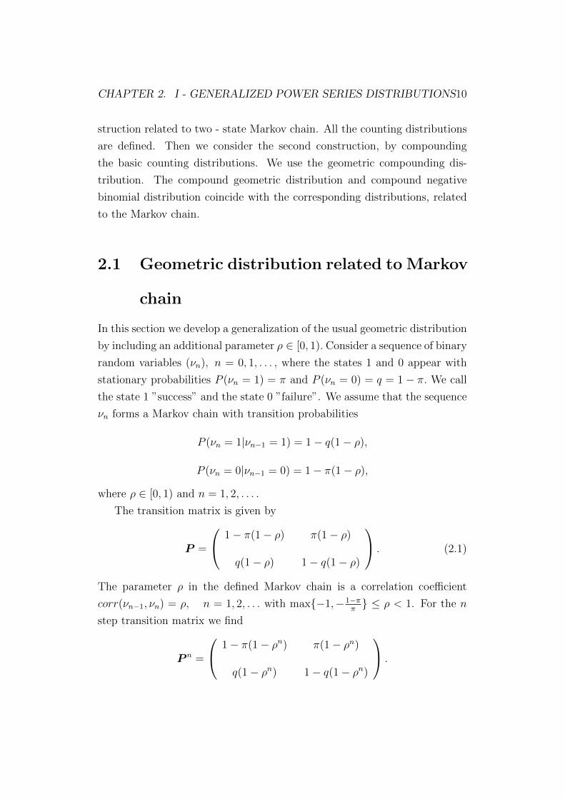
In this section we develop a generalization of the usual geometric distribution
by including an additional parameter ρ ∈ [0, 1). Consider a sequence of binary
random variables (νn), n = 0, 1, . . . , where the states 1 and 0 appear with
stationary probabilities P (νn = 1) = π and P (νn = 0) = q = 1− π. We call
the state 1 ”success” and the state 0 ”failure”. We assume that the sequence
νn forms a Markov chain with transition probabilities
P (νn = 1|νn−1 = 1) = 1− q(1− ρ),
P (νn = 0|νn−1 = 0) = 1− π(1− ρ),
where ρ ∈ [0, 1) and n = 1, 2, . . . .
The transition matrix is given by
P =
1− π(1− ρ) π(1− ρ)
q(1− ρ) 1− q(1− ρ)
. (2.1)
The parameter ρ in the defined Markov chain is a correlation coefficient
corr(νn−1, νn) = ρ, n = 1, 2, . . . with max−1,−1−ππ ≤ ρ < 1. For the n
step transition matrix we find
P n =
1− π(1− ρn) π(1− ρn)
q(1− ρn) 1− q(1− ρn)
.

CHAPTER 2. I - GENERALIZED POWER SERIES DISTRIBUTIONS11
Let the random variable X counts the number of failures in the Markov
chain up to the first success. The PMF and PGF are given by
P (X = k) =
π, k = 0
(1− π)[1− π(1− ρ)]k−1(1− ρ)π, k = 1, 2, . . . ,(2.2)
and
PX(s) =π(1− ρs)
1− (1− π(1− ρ))s. (2.3)
It is easy to verify that the above equations define a proper probability dis-
tribution.
Definition 2.1 The random variable X, defined by (2.2) and (2.3) is said
to be a geometrically distributed related to the Markov chain. We use the
notation IGe(π, ρ).
Remark 2.1 If ρ = 0, the defined geometric distribution coincides with the
usual geometric distribution on the nonnegative integer values, with parame-
ter π, i. e. Ge0(π) ≡ IGe(π, 0).
Remark 2.2 The mean and the variance of the IGe(π, ρ) distribution are
given by
E(X) =1− ππ(1− ρ)
and V ar(X) =(1− π)(1 + πρ)
π2(1− ρ)2.
2.1.1 ρ - Type Lack of Memory Property
It is well known, from Galambos and Kotz [35], that the equation
P (U ≥ b+ x | U ≥ b) = P (U ≥ x), x ≥ 0, b > 0, (2.4)
is true for a random variable U which is nonnegative and non - degenerate at
zero, if and only if it has either the exponential or the geometric distribution.

CHAPTER 2. I - GENERALIZED POWER SERIES DISTRIBUTIONS12
Equation (2.4) is known as the lack of memory property for the random
variable U or for its distribution function.
The following theorem gives the corrected form of the lack of memory
property in the case of IGe distribution.
Theorem 2.1 Let X ∼ IGe(π, ρ). Then for any b > 0, the conditional
probability P (X ≥ b+x |X ≥ b) has the following equivalent representations:
(i) [1− π(1− ρ)]x, x ≥ 0;
(ii) 1−π(1−ρ)1−π P (X ≥ x), x > 0;
(iii) P (X ≥ x) + ρ π1−πP (X ≥ x), x > 0;
(iv) P (X ≥ x) + ρπP (X ≥ x |X > 0), x ≥ 0;
(v) (1− ρ)P (X ≥ x) + ρP (X ≥ x |X > 0), x ≥ 0;
(vi) P (X ≥ x+ 1), x ≥ 0.
Proof. For any fixed integer b ≥ 1 from (2.2) we have
P (X ≥ b) =∞∑k=b
(1− π)π(1− ρ)[1− π(1− ρ)]k−1,
i. e.
P (X ≥ b) = (1− π)[1− π(1− ρ)]b−1.
Then for any x ≥ 0
P (X ≥ b+ x |X ≥ b) =P (X ≥ b+ x)
P (X ≥ b)= [1− π(1− ρ)]x

CHAPTER 2. I - GENERALIZED POWER SERIES DISTRIBUTIONS13
and the representation (i) is obtained.
By simple transformations from (i) one can obtain relations (ii) - (v).
Representation (vi) follows from the definition of the r. v. X and (i).
2
The statement (v) of the Theorem 2.1 gives the reasons of the following
extension of the usual lack - of - memory property.
Definition 2.2 The random variable X has a ρ− type lack - of - memory
property if
P (X ≥ b+ x |X ≥ b) = (1− ρ)P (X ≥ x) + ρP (X ≥ x |X > 0),
for any x > 0 and b > 0.
2.2 Negative binomial distribution related to
a Markov chain
Let r be a positive integer and X1, X2, . . . , Xr be independent identically
distributed (i.i.d.) random variables having IGe(π, ρ) distribution, given by
(2.2).
Define the random variable Y (r) = X1 + . . . + Xr. Since Xi are i.i.d.
random variables, when a success appears, the Markov chain starts again at
the origin and the initial PMF is given by P (νn = 1) = π, P (νn = 0) = 1−π.Let the sequence (νn) denote a Markov chain with the following transition
matrix P∗ :
P∗ =
1− π(1− ρ) π(1− ρ)
1− π π
.
This Markov chain will be called an interrupted Markov chain. The r.
v. Y (r) counts the number of failures up to the rth success in this Markov
chain.

CHAPTER 2. I - GENERALIZED POWER SERIES DISTRIBUTIONS14
The n step transition matrix is given by
P∗n =
1− π(1− ρ)
1− πρ(1− (πρ)n)
π(1− ρ)
1− πρ(1− (πρ)n)
1− π1− πρ
(1− (πρ)n) 1− 1− π1− πρ
(1− (πρ)n)
.
Definition 2.3 We say that the random variable Y (r) = X1 + . . .+Xr has
a negative binomial distribution related to the interrupted Markov chain with
parameters π ∈ (0, 1), ρ ∈ (max−1,−1−ππ, 1) and r ≥ 1. Y (r) is called
also an Inflated - parameter negative binomial distributed with the notation
Y (r) ∼ INB(r, π, ρ).
Since Y (r) is a sum of r i.i.d. random variables, each having a PGF given
by (2.3), the PGF of the random variable Y (r) has the following form
PY (r)(s) =
[π(1− ρs)
1− (1− π + ρπ)s
]r. (2.5)
The PMF of the inflated - parameter negative binomial distribution is
given by the next proposition.
Proposition 2.1 The PMF of the INB(r, π, ρ) distributed random variable
Y (r) is given by the following relation
P (Y (r) = y)
= πr∑
y1, y2, . . .
(y1 + y2 + · · ·+ r − 1
y1, y2, . . . , r − 1
)[(1− π)(1− ρ)]y1+y2+···ρy2+2y3+···,
(2.6)
where y = 0, 1, . . . and the summation is over all nonnegative integers y1, y2, y3, . . . ,
such that y1 + 2y2 + 3y3 + . . . = y.

CHAPTER 2. I - GENERALIZED POWER SERIES DISTRIBUTIONS15
Proof. Using some combinatorial equations, from the PGF (2.5) we obtain
PY (r)(s) =
[π(1− sρ)
1− s(1− π + ρπ)
]r=
πr[1− (1− π)(1− ρ)s 1
1−sρ
]r= πr
∞∑i=0
(i+ r − 1
i
)[(1− π)(1− ρ)s(1 + ρs+ (ρs)2 + . . .)
]i
= πr∞∑i=0
(i+ r − 1
i
)[(1− π)(1− ρ)s]i
∑i1, i2, . . .
(i
i1, i2, . . .
)(ρs)i2+2i3+...,
where the summation is over all nonnegative integers i1, i2, i3, . . ., such that
i1 + i2 + i3 + . . . = i. Now, taking into account the equality(i+ r − 1
i
)(i
i1, i2, . . .
)=
(i+ r − 1
i1, i2, . . . , r − 1
)we have
PY (r)(s) = πr∞∑i=0
[(1− π)(1− ρ)s]i∑
i1, i2, . . .
(i+ r − 1
i1, i2, . . . , r − 1
)(ρs)i2+2i3+....
Substituting in the last expression ij = yj, j ≥ 1 and i = y−∑∞
j=1(j−1)yj
we obtain
PY (r)(s) =∞∑y=0
tyP (Y = y),
where the probability P (Y = y) is given by (2.6) for y ≥ 0.
2
Remark 2.3 In the case ρ = 0 in (2.6), we obtain the PMF of the usual NB
distribution.
Remark 2.4 The probabilities of the first four values of the random variable

CHAPTER 2. I - GENERALIZED POWER SERIES DISTRIBUTIONS16
Y (r) ∼ INB(r, π, ρ) are given by the following expressions
P (Y (r) = 0) = πr,
P (Y (r) = 1) = πrr(1− π)(1− ρ),
P (Y (r) = 2) = πr(1− ρ)(1− π)[(r+1
2
)(1− ρ)(1− π) + rρ
],
P (Y (r) = 3) = πr(1− ρ)(1− π)
×[(r+2
3
)(1− ρ)2(1− π)2 + r(r + 1)(1− ρ)(1− π)ρ+ rρ2
],
derived from (2.6).
Remark 2.5 The mean and the variance of the INB(π, ρ, r) distribution
are given by
E(Y (r)) =r(1− π)
π(1− ρ)and V ar(Y (r)) =
r(1− π)(1 + πρ)
π2(1− ρ)2.
2.3 Poisson limiting distribution
Here we will obtain the PGF and PMF of a new distribution, by finding the
limits of the expressions (2.5) and (2.6) when
r −→∞ and π −→ 1, such that r(1− π) = λ = const > 0.(2.7)
The limiting PGF is given by the following proposition.
Proposition 2.2 Under the limiting conditions (2.7) the following relation
is true
limr→∞
limπ→1
PY (r)(s) = exp
[λ(s− 1)
1− sρ
], (2.8)
where PY (r)(s) is the PGF given by (2.5).
Proof. Taking logarithm on both sides of (2.5) we have
lnPY (r)(s) = r ln[1− (1− π + ρπs)]− ln[1− (1− π + ρπ)s] .

CHAPTER 2. I - GENERALIZED POWER SERIES DISTRIBUTIONS17
Using the Taylor expansion of the logarithmic function ln(1− x), after some
simple transformations we obtain that
lnPY (r)(s) = r(1− π)(s− 1)
1 +
1
2[2ρπs+ (1− π)(s+ 1)]
+1
3[3(ρπs)2 + 3ρπ(1− π)s(s+ 1) + (1− π)2(s2 + s+ 1)] + . . .
.
Now using the limiting conditions (2.7) we have
limr→∞
limπ→1
lnPY (r)(s) = λ(s− 1)[1 + ρs+ (ρs)2 + · · · ] =λ(s− 1)
1− ρs.
Taking anti - logarithm in the last relation we obtain (2.8).
2
Remark 2.6 In the case of ρ = 0, the limiting PGF given (2.8) coincides
with the PGF of the usual Poisson distribution with parameter λ > 0.
This motivate the following definition.
Definition 2.4 The random variable Z defined by the PGF
PZ(s) = exp
[λ(s− 1)
1− ρs
]. (2.9)
has a Poisson distribution related to the Markov chain with parameters λ > 0
and ρ ∈ [0, 1). It is called also Inflated - parameter Poisson distribution
(Z ∼ IPo(λ, ρ)).
By analogy with the NB case, we will obtain the PMF of the IPo(λ, ρ)
distribution by the following proposition.
Proposition 2.3 The PMF of the IPo(λ, ρ) distributed random variable Z
is given by the following relation
P (Z = z) =∑
z1, z2, . . .
e−λ
z1!z2! . . .[λ(1− ρ)]z1+z2+···ρz2+2z3+···, (2.10)

CHAPTER 2. I - GENERALIZED POWER SERIES DISTRIBUTIONS18
where z = 0, 1, . . . and the summation is over all nonnegative integers z1, z2, z3, . . .
such that
z1 + 2z2 + 3z3 + · · · = z.
Proof. From the PGF (2.9) we have
PZ(s) = exp[λ(s− 1)(1 + ρs+ ρ2s2 + . . .)
]= exp
λ[−1 + (1− ρ)s+ ρ(1− ρ)s2 + ρ2(1− ρ)s3 + . . .]
.
Using the Taylor expansion of the exponential function exp(x), we obtain
PZ(s) =∞∑n=0
λn[−1 + (1− ρ)s+ ρ(1− ρ)s2 + ρ2(1− ρ)s3 + · · · ]n
n!,
i. e.
PZ(s)
=∞∑n=0
λn
n!
∑n0, n1, . . .
(n
n0, n1, . . .
)(−1)n0(1− ρ)n1+n2+···ρn2+2n3+···sn1+2n2+3n3+···,
where the summation is over all nonnegative integers n0, n1, n2, . . ., such that
n0 + n1 + n2 + · · · = n. Substituting in the last expression ni = zi, i ≥ 0
and n = z −∑∞
j=0(j − 1)zj we obtain
PZ(s) =∞∑z=0
sz∑
z1, z2, . . .
[λ(1− ρ)]z1+z2+···ρz2+2z3+···
z1!z2! . . .
∞∑z0=0
(−λ)z0
z0!,
where z = 0, 1, . . . and the summation is over all nonnegative integers z1, z2, z3, . . .
such that z1 + 2z2 + 3z3 + · · · = z. Therefore,
PZ(s) =∞∑z=0
szP (Z = z),
where the probability P (Z = z) is given by (2.10) for z ≥ 0.
2

CHAPTER 2. I - GENERALIZED POWER SERIES DISTRIBUTIONS19
Remark 2.7 From (2.10) we obtain the probabilities of the first four values
of Z ∼ IPo(λ, ρ), given by the following expressions
P (Z = 0) = e−λ,
P (Z = 1) = e−λλ(1− ρ),
P (Z = 2) = e−λλ(1− ρ)[λ(1−ρ)
2!+ ρ],
P (Z = 3) = e−λλ(1− ρ)[λ2(1−ρ)2
3!+ λ(1− ρ)ρ+ ρ2
].
Remark 2.8 We will show how to obtain the PMF (2.10) of the inflated -
parameter Poisson random variable from the PMF (2.6) of the INB distribu-
tion by using the limiting conditions (2.7).
It is easy to show that the following equality is true(y1 + y2 + . . . s+ r − 1
y1, y2, . . . , r − 1
)
=∞∏i=1
(r − 1 + yi)(r − 1 + yi − 1) · · · [r − 1 + yi − (yi − 1)]
yi!=∞∏i=1
Ai.
Then (2.6) can be represented as
P (Y (r) = y) = πr∑
y1, y2, . . .(1−ρ)y1+y2+···ρy2+2y3+···A1(1−π)y1
∞∏i=2
Ai(1−π)yi ,
Under the limiting conditions (2.7) the following two relations
limr→∞
limπ→1
πr = limr→∞
(1− λ
r
)r= e−λ and lim
r→∞(1−π)yi =
λyi
ryi, i = 1, 2, . . .
are valid. Then
limr→∞
limπ→1
A1πr(1− π)y1 =
e−λλy1
y1!and lim
r→∞limπ→1
Ai =λyi
yi!, i = 2, 3, . . .
Therefore,
limr→∞
limπ→1
P (Y (r) = y) = P (Z = z),
where P (Z = z) is given by (2.10) for z = 0, 1, . . ..
CHAPTER 2. I - GENERALIZED POWER SERIES DISTRIBUTIONS20
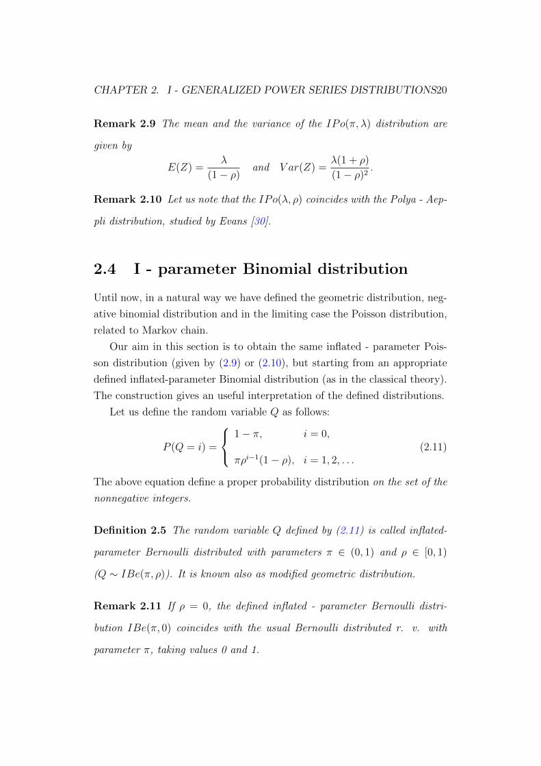
Remark 2.9 The mean and the variance of the IPo(π, λ) distribution are
given by
E(Z) =λ
(1− ρ)and V ar(Z) =
λ(1 + ρ)
(1− ρ)2.
Remark 2.10 Let us note that the IPo(λ, ρ) coincides with the Polya - Aep-
pli distribution, studied by Evans [30].
2.4 I - parameter Binomial distribution
Until now, in a natural way we have defined the geometric distribution, neg-
ative binomial distribution and in the limiting case the Poisson distribution,
related to Markov chain.
Our aim in this section is to obtain the same inflated - parameter Pois-
son distribution (given by (2.9) or (2.10), but starting from an appropriate
defined inflated-parameter Binomial distribution (as in the classical theory).
The construction gives an useful interpretation of the defined distributions.
Let us define the random variable Q as follows:
P (Q = i) =
1− π, i = 0,
πρi−1(1− ρ), i = 1, 2, . . .(2.11)
The above equation define a proper probability distribution on the set of the
nonnegative integers.
Definition 2.5 The random variable Q defined by (2.11) is called inflated-
parameter Bernoulli distributed with parameters π ∈ (0, 1) and ρ ∈ [0, 1)
(Q ∼ IBe(π, ρ)). It is known also as modified geometric distribution.
Remark 2.11 If ρ = 0, the defined inflated - parameter Bernoulli distri-
bution IBe(π, 0) coincides with the usual Bernoulli distributed r. v. with
parameter π, taking values 0 and 1.

CHAPTER 2. I - GENERALIZED POWER SERIES DISTRIBUTIONS21
From (2.11) we calculate the corresponding PGF PQ(s) given by the fol-
lowing expression
PQ(s) = 1− π(1− s)1− ρs
. (2.12)
Now, if we sum n i.i.d. IBe(π, ρ) random variables we will obtain the
random variable B with the following PGF
PB(s) =
[1− π(1− s)
1− ρs
]n. (2.13)
Definition 2.6 We call the random variable B defined by the PGF (2.13)
inflated - parameter binomial distributed with parameters π ∈ (0, 1), ρ ∈ [0, 1)
and n, and will denote this by B ∼ IBi(n, π, ρ).
The next proposition represents the PMF of the IBi(n, π, ρ) distributed
random variable
Proposition 2.4 The PMF of the IBi(n, π, ρ) distributed random variable
B is given by the following relation
P (B = b) = (1−π)n∑
b1, b2, . . .
(n
n− b1 − b2 − . . . , b1, b2, . . .
)ρb[π(1− ρ)
(1− π)ρ
]b1+b2+...
,
(2.14)
where b = 0, 1, . . . and the summation is over all nonnegative integers b1, b2, b3 . . .
such that
b1 + 2b2 + 3b3 . . . = b.

CHAPTER 2. I - GENERALIZED POWER SERIES DISTRIBUTIONS22
Proof. From the PGF (2.14) we consequently obtain
PB(s) =
[1− π +
π(1− ρ)s
1− ρs
]n
= (1− π)nn∑k=0
(n
k
)[π(1− ρ)ρs
ρ(1− π)(1− ρs)
]k
= (1− π)nn∑k=0
(n
k
)[π(1− ρ)
ρ(1− π)(ρs+ ρ2s2 + . . .)
]k
= (1− π)nn∑k=0
(n
k
) ∑k1, k2, . . .
(k
k1, k2, . . .
)[π(1− ρ)
ρ(1− π)
]k1+k2+...
(ρs)k1+2k2+...,
where the summation is over all nonnegative integers k1, k2, . . ., such that
k1 + k2 + · · · = k. Substituting in the last expression ki = bi, i ≥ 1 and
k = b−∑∞
j=1(j − 1)bj we obtain
PB(s) =∞∑b=0
sbP (B = b),
where the probability P (B = b) is given by (2.14) for b ≥ 0.
2
Remark 2.12 Representation (2.14) has the following equivalent form:
P (B = b) =∑
b1, b2, . . .
(n
n0, b1, b2, . . .
)(1− π)n0 [π(1− ρ)]b1+b2+...ρb2+2b3+...,
(2.15)
with b = 0, 1, . . . and summation over all nonnegative integers b1, b2, b3, . . .,
such that b1 + 2b2 + 3b3 + . . . = b, under condition that n0 + b1 + b2 + . . . = n.
Remark 2.13 Let us note that the defined IBi(π, ρ, n) distributed random
variable can take infinite number of non-negative values, since by construction
the corresponding inflated - parameter Bernoulli distributed random variable
can take all non-negative integer values.
CHAPTER 2. I - GENERALIZED POWER SERIES DISTRIBUTIONS23
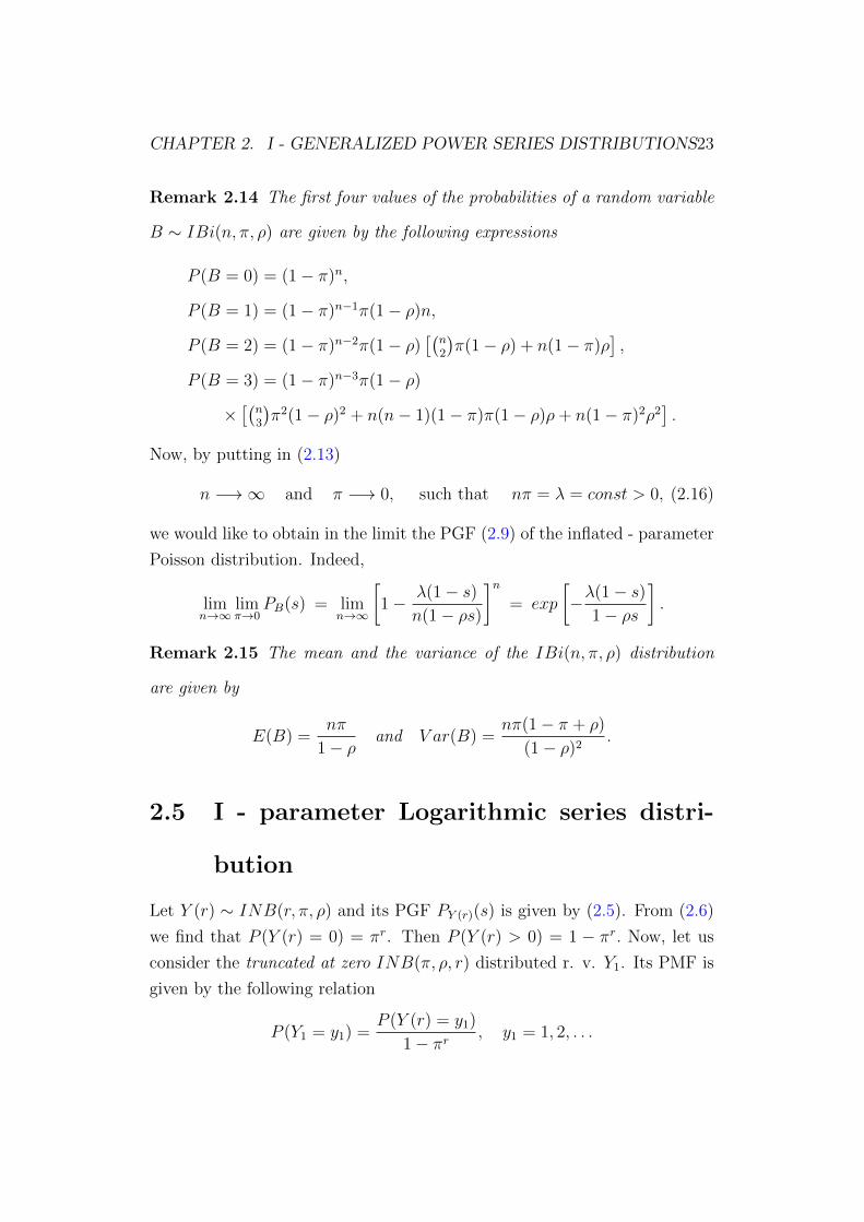
Remark 2.14 The first four values of the probabilities of a random variable
B ∼ IBi(n, π, ρ) are given by the following expressions
P (B = 0) = (1− π)n,
P (B = 1) = (1− π)n−1π(1− ρ)n,
P (B = 2) = (1− π)n−2π(1− ρ)[(n2
)π(1− ρ) + n(1− π)ρ
],
P (B = 3) = (1− π)n−3π(1− ρ)
×[(n3
)π2(1− ρ)2 + n(n− 1)(1− π)π(1− ρ)ρ+ n(1− π)2ρ2
].
Now, by putting in (2.13)
n −→∞ and π −→ 0, such that nπ = λ = const > 0, (2.16)
we would like to obtain in the limit the PGF (2.9) of the inflated - parameter
Poisson distribution. Indeed,
limn→∞
limπ→0
PB(s) = limn→∞
[1− λ(1− s)
n(1− ρs)
]n= exp
[−λ(1− s)
1− ρs
].
Remark 2.15 The mean and the variance of the IBi(n, π, ρ) distribution
are given by
E(B) =nπ
1− ρand V ar(B) =
nπ(1− π + ρ)
(1− ρ)2.
2.5 I - parameter Logarithmic series distri-
bution
Let Y (r) ∼ INB(r, π, ρ) and its PGF PY (r)(s) is given by (2.5). From (2.6)
we find that P (Y (r) = 0) = πr. Then P (Y (r) > 0) = 1 − πr. Now, let us
consider the truncated at zero INB(π, ρ, r) distributed r. v. Y1. Its PMF is
given by the following relation
P (Y1 = y1) =P (Y (r) = y1)
1− πr, y1 = 1, 2, . . .

CHAPTER 2. I - GENERALIZED POWER SERIES DISTRIBUTIONS24
The corresponding PGF PY1(s) has the form
PY1(s) =1
1− πr[PY (r)(s)− πr
]=
πr
1− πr
(1− ρs)r − [1− s(1− π + ρπ)]r
[1− s(1− π + ρπ)]r
.
Assuming r → 0 in the last expression, after using the L’Hopital’s rule,
we obtain the relation
limr→0
PY1(s) = ln
[1− ρs
1− s(1− π + ρπ)
](− ln π)−1.
If we denote by L the random variable having the limiting PGF, then the
following equality is fulfilled
PL(s) = ln
[1 +
(1− π)(1− ρ)s
1− s(1− π + ρπ)
](− lnπ)−1.
After simple transformations, the PGF PL(s) can be given by the follow-
ing equivalent representation
PL(s) = ln
[1− (1− π)(1− ρ)s
1− ρs
]−1
(− lnπ)−1. (2.17)
Remark 2.16 If we put ρ = 0 in the last expression, we derive the PGF of
the usual logarithmic series distribution.
So, we are ready to give the following definition.
Definition 2.7 The random variable L defined by the PGF (2.17) is called
inflated - parameter logarithmic series distribution with parameters π ∈ (0, 1)
and ρ ∈ [0, 1). We denote this by L ∼ ILS(π, ρ).
The following proposition represents the PMF of the defined inflated -
parameter logarithmic series distribution.
Proposition 2.5 The PMF of the ILS(π, ρ) distributed random variable L
is given by the following relation
P (L = l) =∑
l1, l2, . . .
(−1 + l1 + l2 + . . .)!
(− lnπ)l1!l2! . . .[(1− π)(1− ρ)]l1+l2+...ρl2+2l3+...,
(2.18)
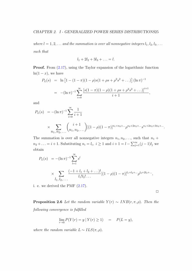
CHAPTER 2. I - GENERALIZED POWER SERIES DISTRIBUTIONS25
where l = 1, 2, . . . and the summation is over all nonnegative integers l1, l2, l3, . . .
such that
l1 + 2l2 + 3l3 + . . . = l.
Proof. From (2.17), using the Taylor expansion of the logarithmic function
ln(1− x), we have
PL(s) = ln[1− (1− π)(1− ρ)s(1 + ρs+ ρ2s2 + . . .)
](ln π)−1
= −(lnπ)−1
∞∑i=0
[s(1− π)(1− ρ)(1 + ρs+ ρ2s2 + . . .)]i+1
i+ 1,
and
PL(s) = −(ln π)−1
∞∑i=0
1
i+ 1
×∑
n1, n2, . . .
(i+ 1
n1, n2, . . .
)[(1− ρ)(1− π)]n1+n2+...ρn2+2n3+...sn1+2n2+3n3+....
The summation is over all nonnegative integers n1, n2, . . ., such that n1 +
n2 + . . . = i+ 1. Substituting ni = li, i ≥ 1 and i+ 1 = l−∑∞
j=1(j − 1)lj we
obtain
PL(s) = −(ln π)−1
∞∑l=1
sl
×∑
l1, l2, . . .
(−1 + l1 + l2 + . . .)!
l1!l2! . . .[(1− ρ)(1− π)]l1+l2+...ρl2+2l3+...,
i. e. we derived the PMF (2.17).
2
Proposition 2.6 Let the random variable Y (r) ∼ INB(r, π, ρ). Then the
following convergence is fulfilled
limr→0
P (Y (r) = y | Y (r) ≥ 1) = P (L = y),
where the random variable L ∼ ILS(π, ρ).

CHAPTER 2. I - GENERALIZED POWER SERIES DISTRIBUTIONS26
Proof. Since P (Y (r) ≥ 1) = 1− πr, we have
P (Y (r) = y | Y (r) ≥ 1) =P (Y (r) = y, Y (r) ≥ 1)
P (Y (r) ≥ 1)
=P (Y (r) = y, Y (r) ≥ 1)
1− πr.
From the last relation and (2.5) we have
P (Y (r) = y|Y (r) ≥ 1)
=πr
1− πr∑
y1, y2, . . .
(y1 + y2 + . . .+ r − 1
y1, y2, . . . , r − 1
)[(1− π)(1− ρ)]y1+y2+...ρy2+2y3+...
=rπr
1− πr∑
y1, y2, . . .
(y1 + y2 + . . .+ r − 1) . . . (r + 2)(r + 1)
y1!y2! . . .
×[(1− π)(1− ρ)]y1+y2+...ρy2+2y3+....
Notice that according to the L’Hopital’s rule limr→0
rπr
1−πr = −(ln π)−1. Then
it can be seen that limr→0
P (Y (r) = y|Y (r) ≥ 1) converges to the PMF P (L =
y), y = 1, 2, . . . of the inflated - parameter logarithmic series distribution as
given by (2.17).
2
Remark 2.17 The univariate NB and logarithmic series distributions are
related with the same limiting results stated by the last two propositions, see
Qu et al. (1990), [75].
Remark 2.18 The probabilities of the first three values of the random vari-
able L ∼ ILS(π, ρ), are given by the following expressions
P (L = 1) = −(ln π)−1(1− ρ)(1− π),
P (L = 2) = −(ln π)−1(1− ρ)(1− π)[
(1−ρ)(1−π)2
+ ρ],
P (L = 3) = −(ln π)−1(1− ρ)(1− π)[
(1−ρ)2(1−π)2
3+ (1− ρ)(1− π)ρ+ ρ2
].
CHAPTER 2. I - GENERALIZED POWER SERIES DISTRIBUTIONS27
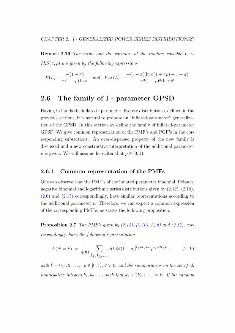
Remark 2.19 The mean and the variance of the random variable L ∼
ILS(π, ρ) are given by the following expressions
E(L) =−(1− π)
π(1− ρ) lnπand V ar(L) =
−(1− π)[lnπ(1 + πρ) + 1− π]
π2(1− ρ)2(lnπ)2.
2.6 The family of I - parameter GPSD
Having in hands the inflated - parameter discrete distributions, defined in the
previous sections, it is natural to propose an ”inflated-parameter” generaliza-
tion of the GPSD. In this section we define the family of inflated-parameter
GPSD. We give common representation of the PMF’s and PGF’s in the cor-
responding subsections. An over-dispersed property of the new family is
discussed and a new constructive interpretation of the additional parameter
ρ is given. We will assume hereafter that ρ ∈ [0, 1).
2.6.1 Common representation of the PMFs
One can observe that the PMF’s of the inflated-parameter binomial, Poisson,
negative binomial and logarithmic series distributions given by (2.12), (2.10),
(2.6) and (2.17) correspondingly, have similar representations according to
the additional parameter ρ. Therefore, we can expect a common expression
of the corresponding PMF’s, as states the following proposition.
Proposition 2.7 The PMF’s given by (2.14), (2.10), (2.6) and (2.17), cor-
respondingly, have the following representation
P (N = k) =1
g(θ)
∑k1, k2, . . .
a(k)[θ(1− ρ)]k1+k2+···ρk2+2k3+..., (2.19)
with k = 0, 1, 2, . . . , ρ ∈ [0, 1), θ > 0, and the summation is on the set of all
nonnegative integers k1, k2, . . ., such that k1 + 2k2 + . . . = k. If the random

CHAPTER 2. I - GENERALIZED POWER SERIES DISTRIBUTIONS28
variable X ∼ ILS(θ, ρ), its values begin from 1 and the summation in (2.19)
is over nonnegative integers, such that k1 + 2k2 + . . . = k + 1.
In the particular cases, the functions a(k), g(θ) and the parameter θ, are
given by the following expressions
N ∼ IPo(θ, ρ) : a(k) = 1k1!k2!...
, g(θ) = eθ, θ = λ,
N ∼ INB(θ, ρ, r) : a(k) =(k1+k2+...+r−1k1,k2,...,r−1
), g(θ) = (1− θ)−r, θ = 1− π,
N ∼ IBi(θ, ρ, n) : a(k) =(
nn−k1−k2−...,k1,k2,...
), g(θ) = (1 + θ)n, θ = π
1−π ,
N ∼ ILS(θ, ρ) : a(k) = (−1+k1+k2+...)!k1!k2!...
, g(θ) = − ln(1− θ), θ = 1− π.
Proof. Using simple transformations one can obtain the above relations
from (2.10), (2.6), (2.14) and (2.18), respectively.
2
Definition 2.8 The random variable N belongs to the family of Inflated -
parameter GPSD with parameters θ > 0 and ρ ∈ [0, 1) if its PMF can be
represented by (2.19).
Remark 2.20 Let us note that the defined family is different than the cor-
responding family studied by Gupta et al. [40].
2.6.2 Explicit expressions for PMFs
The PMF’s given by Proposition 2.7 can be represented by alternative explicit
expressions, which are given by the following

CHAPTER 2. I - GENERALIZED POWER SERIES DISTRIBUTIONS29
Proposition 2.8 The PMF’s of the IPo(θ, ρ), INB(r, θ, ρ), IBi(n, θ, ρ) and
ILS(θ, ρ) distributed random variables can be given by the following equiva-
lent expressions
(i) P (N = k) =
e−λ, k = 0
e−λ∑k
i=1
(k−1i−1
) [λ(1−ρ)]i
i!ρk−i, k = 1, 2, . . . ,
if N has the Inflated - parameter Poisson distribution with parameters
λ > 0 and ρ, say N ∼ IPo(λ, ρ);
(ii) P (N = k) =
πr, k = 0
πr∑k
i=1
(k−1i−1
)(r+i−1i
)[(1− π)(1− ρ)]iρk−i, k = 1, 2, . . . ,
if N has the Inflated - parameter Negative binomial distribution with
parameters π ∈ (0, 1), ρ and r > 0, say N ∼ INB(π, ρ, r);
(iii) P (N = k) =
(1− π)n, k = 0min(k,n)∑i=1
(n
i
)(k − 1
i− 1
)[π(1− ρ)]i(1− π)n−iρk−i, k = 1, 2, . . . ,
if N has the Inflated - parameter Binomial distribution with parameters
π ∈ (0, 1), ρ and n ∈ 1, 2, . . ., say N ∼ IBi(π, ρ, n).
When n = 1, we obtain the Inflated - parameter Bernoulli r. v. with
parameters π and ρ;
(iv) P (N = k) = (−lnπ)−1
k∑i=1
(k − 1
i− 1
)[(1− π)(1− ρ)]iρk−i
i, k = 1, 2, . . . ,
if N has the Inflated - parameter logarithmic-series distribution with
parameters π ∈ (0, 1) and ρ, say N ∼ ILS(π, ρ).

CHAPTER 2. I - GENERALIZED POWER SERIES DISTRIBUTIONS30
(v) P (N = k) =
π, k = 0
(1− π)[1− π(1− ρ)]k−1(1− ρ)π, k = 1, 2, . . . ,
if N has the Inflated - parameter geometric distribution, say N ∼
IGe(π, ρ). The IGe(π, ρ) distribution is in fact the INB(π, ρ, 1).
Proof. We will demonstrate how to obtain the PMF for the random variable
N ∼ IPo(λ, ρ). The remaining expressions can be deduced in a similar way.
The starting point here is to use the following relation
1
(1− y)j=∞∑l=0
(l + j − 1
l
)yl, 0 < y < 1, (2.20)
valid for any j = 1, 2, . . ..
For the PGF (2.9) we have
PN(s) = expλ[−1 + (1− ρ)s+ ρ(1− ρ)s2 + ρ2(1− ρ)s3 + . . .]
.
Using the Taylor expansion of the exponential function exp(x), after some
algebra we obtain
PN(s) = e−λ
1 +
∞∑j=1
[λ(1− ρ)s]j
j!
1
(1− ρs)j
.
Applying (2.20) in the above expression we have
∞∑m=0
P (N = m)sm = e−λ
1 +
∞∑j=1
[λ(1− ρ)s]j
j!
∞∑l=0
(l + j − 1
l
)ρlsl
.
The PMF of the random variable N ∼ IPo(λ, ρ) given by the proposition is
obtained by equating the coefficients of sm on both sides of the last equality
for fixed m = 0, 1, 2, . . . .
2
2.7 The PGF of the family of IGPSDs
Let PY (s) and PX(s) be PGF’s of the non-negative integer valued random
variables Y and X, respectively. Then the resulting function PY (PX(s)), is

CHAPTER 2. I - GENERALIZED POWER SERIES DISTRIBUTIONS31
also a PGF, corresponding to the sum of independent identically distributed
random variables having a PGF PX(s), where the number of summands is
independent of the random variables and has a PGF PY (s).
This situation describes the portfolio of insurance policies during a given
length of time. Let N denote the number of claims and let Xi denote the
amount of the i-th claim. Let X1, X2, . . . be a sequence of independent and
identically distributed random variables with common PGF PX(s). Assume
that Xi, i = 1, 2, . . . are also independent on N and consider the random
sum
N = X1 +X2 + . . .+XY ,
with the convention that N = 0 if Y = 0. Then N equals aggregate claims,
and the corresponding PGF PN(s) is just PY (PX(s)), see for example Bowers
et al. [15].
Now, if Y belongs to the family of GPSD with parameter θ defined by
(2.1) and X is an arbitrary discrete distribution, then the resulting random
sum S has a PGF given by the following expression
PN(s) =g(θPX(s))
g(θ), (2.21)
where the possible choices of the function g(·) are given in the Proposition
2.7, see Hirano et al. [42] also.
After the inflated - parameter binomial, Poisson, NB and logarithmic
series distributions have a common representation for their PMF’s one can
expect that they have the corresponding common representation of their
PGF’s. This is precised by the following statement, which gives the PGF of
the inflated - parameter GPSD defined by Definition 2.8.
Proposition 2.9 The PGF of the inflated - parameter GPSD is given by
(2.21), where the functions g(θ) are given by Proposition 2.7 and
PX(s) =(1− ρ)s
1− ρs. (2.22)

CHAPTER 2. I - GENERALIZED POWER SERIES DISTRIBUTIONS32
Proof. Using simple transformations from the corresponding functions g(θ),
given by Proposition 2.7, relations (2.21) and (2.22), one can get easy the
PGF’s (2.13), (2.9), (2.5) and (2.17), respectively.
2
In fact, Proposition 2.9 gives a constructive representation of the distri-
butions belonging to the family of inflated-parameter GPSD. Indeed, (2.22)
is the PGF of the geometric distribution with parameter 1 − ρ and taking
positive integer values. It gives also a new interpretation of the additional
parameter ρ, different than the correlation coefficient for the Markov chain,
as discussed earlier.
In terms of the collective risk model, this means that the aggregated claim
S has inflated-parameter GPSD when the individual claims have geometric
distribution with parameter 1−ρ, i.e. Xi ∼ Ge1(1−ρ), and number of claims
N for a given length of time is a r.v. belonging to the usual family of GPSD
with parameter θ.
Remark 2.21 From (2.21) and (1.3) it is easy to establish, that the variance-
mean ratio of the inflated - parameter GPSD is greater than the corresponding
variance - mean ratio of the original GPSD. This means that the new family
is over - dispersed relative to the family of GPSD, if the additional parameter
ρ ∈ (0, 1).
2.8 Compound Generalized Power series dis-
tributions
According to the Proposition 2.9, the family of IGPSDs can be defined as a
Compound GPSDs.
Let us suppose that the random variable X has the shifted geometric
distribution Ge1(1− ρ) with parameter ρ ∈ [0, 1), probability mass function
P (X = k) = ρk−1(1− ρ), k = 1, 2, 3, . . . (2.23)

CHAPTER 2. I - GENERALIZED POWER SERIES DISTRIBUTIONS33
and the PGF given by (2.22).
Let the discrete random variable N with parameters θ and ρ has the
following PGF
PN(t) =g(θPX(t))
g(θ), (2.24)
where the series function g(θ) is a positive, finite and differentiable. We are
ready to give the next definition.
Definition 2.9 The random variable N belongs to the family of Inflated -
parameter Power Series Distributions (IPSD), if it is defined on the non -
negative integers and has the PGF given by (2.24).
Definition 2.10 The random variable N belongs to the family of Inflated -
parameter Generalized Power Series Distributions (IGPSD), if it is defined
on any subset of the non - negative integers and has the PGF given by (2.24).
Remark 2.22 It is clear that IPSD ⊂ IGPSD.
Example 2.1 The first three distributions in the previous section belong to
the family of IPSD. The corresponding series functions and parameters are
the following (see [20])
N ∼ IPo(θ, ρ) : g(θ) = eθ, θ = λ,
N ∼ INB(θ, ρ, r) : g(θ) = (1− θ)−r, θ = 1− π,
N ∼ IBi(θ, ρ, n) : g(θ) = (1 + θ)n, θ = π1−π .
Example 2.2 The Inflated - parameter logarithmic - series distribution be-
longs to the family of IGPSD, but not to IPSD:
N ∼ ILS(θ, ρ) : g(θ) = − ln(1− θ), θ = 1− π.

CHAPTER 2. I - GENERALIZED POWER SERIES DISTRIBUTIONS34
The definitions 2.9 and 2.10 give a constructive representation of the dis-
tributions belonging to the family of IGPSD. Let X1, X2, . . . be independent,
identically geometric distributed random variables, having the probability
mass function (2.23). The random variable Y belongs to the usual family of
GPSD with parameter θ > 0 and Y be independent of the above sequence.
Then the random sum X1 +X2 + . . .+XY has a PGF given by (2.24).
Using the above interpretation we will give the next representation of the
PMF of the IGPSD.
It is well known that the sum of m independent, geometrically distributed
random variables is a negative binomial distributed random variable, i.e. if
we denote Sm = X1 + . . .+Xm, then
P (Sm = k) =
(k − 1
m− 1
)(1− ρ)mρk−m, k = m,m+ 1, . . . (2.25)
Let us note another useful interpretation of the model. If we suppose
that any insurance policy produces two types of claims named ”success”
with probability 1 − ρ and ”failure” with probability ρ, then the r.v. Sm
represents the total number of claims until the m-th successive claim ap-
pears. The parameter m in (2.25) is equal to the number of geometrically
distributed random variables. We suppose that m is an outcome from the
random variable Y independent of X1, X2, . . .. Then Sm has the mixed
Negative binomial distribution. If Y is discrete distributed random variable
and pm = P (Y = m), m ∈ S, where S is any nonempty enumerable set of
nonnegative integers, then
P (SY = k) =∑m∈S
(k − 1
m− 1
)(1− ρ)mρk−m pm, k = m,m+ 1, . . . . (2.26)
According to the above interpretation, by suitable choice of the random
variable Y , (2.26) leads up to the PMF’s of the IGPSD. This means that
the Inflated - parameter distributions are mixed negative binomial distri-
butions. Moreover the PMF’s can be presented in terms of the Gaussian
hypergeometric function and the Confluent hypergeometric function given in
the Appendix. The PMF of the Inflated-parameter logarithmic-series dis-
tribution has an explicit expression. This is the statement of the following
Proposition.
CHAPTER 2. I - GENERALIZED POWER SERIES DISTRIBUTIONS35
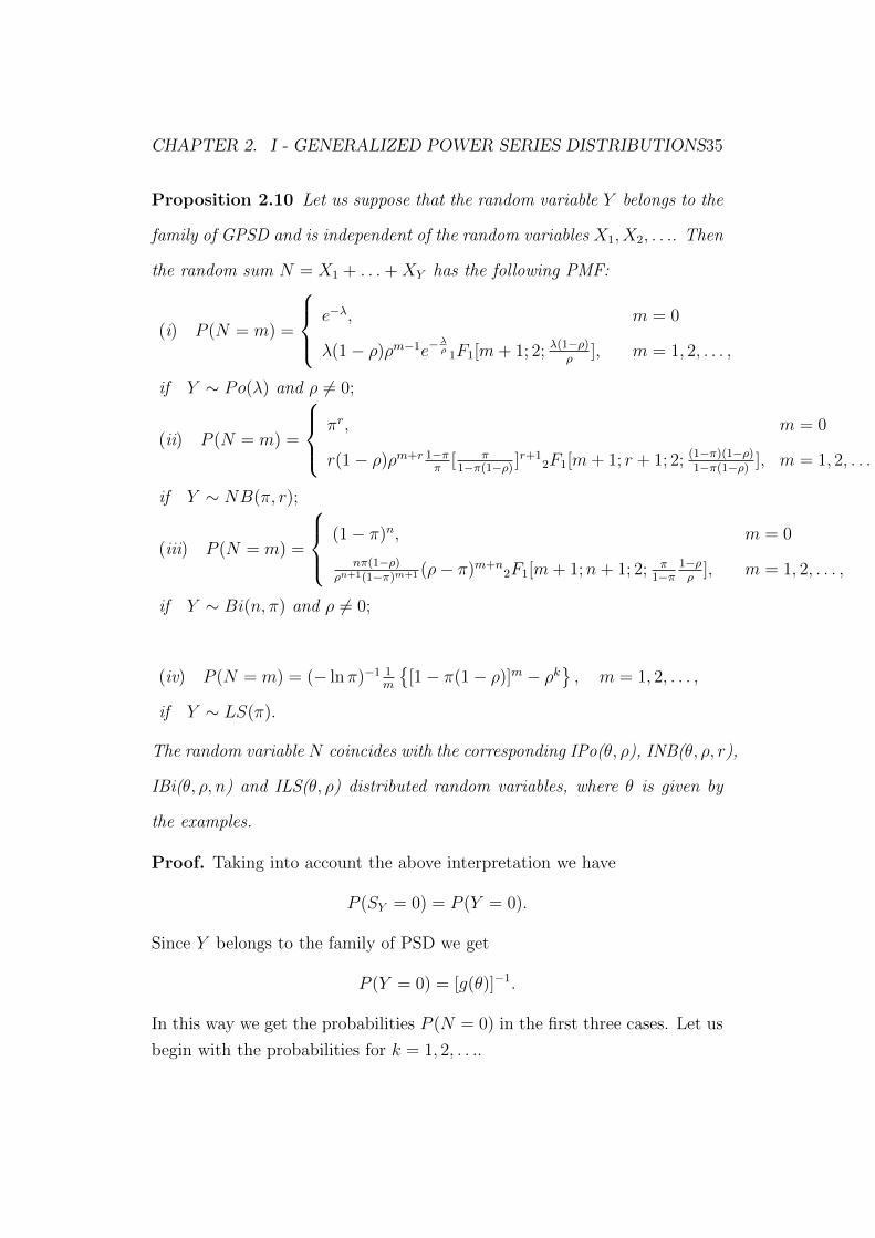
Proposition 2.10 Let us suppose that the random variable Y belongs to the
family of GPSD and is independent of the random variables X1, X2, . . .. Then
the random sum N = X1 + . . .+XY has the following PMF:
(i) P (N = m) =
e−λ, m = 0
λ(1− ρ)ρm−1e−λρ
1F1[m+ 1; 2; λ(1−ρ)ρ
], m = 1, 2, . . . ,
if Y ∼ Po(λ) and ρ 6= 0;
(ii) P (N = m) =
πr, m = 0
r(1− ρ)ρm+r 1−ππ
[ π1−π(1−ρ)
]r+12F1[m+ 1; r + 1; 2; (1−π)(1−ρ)
1−π(1−ρ)], m = 1, 2, . . . ,
if Y ∼ NB(π, r);
(iii) P (N = m) =
(1− π)n, m = 0
nπ(1−ρ)ρn+1(1−π)m+1 (ρ− π)m+n
2F1[m+ 1;n+ 1; 2; π1−π
1−ρρ
], m = 1, 2, . . . ,
if Y ∼ Bi(n, π) and ρ 6= 0;
(iv) P (N = m) = (− ln π)−1 1m
[1− π(1− ρ)]m − ρk
, m = 1, 2, . . . ,
if Y ∼ LS(π).
The random variable N coincides with the corresponding IPo(θ, ρ), INB(θ, ρ, r),
IBi(θ, ρ, n) and ILS(θ, ρ) distributed random variables, where θ is given by
the examples.
Proof. Taking into account the above interpretation we have
P (SY = 0) = P (Y = 0).
Since Y belongs to the family of PSD we get
P (Y = 0) = [g(θ)]−1.
In this way we get the probabilities P (N = 0) in the first three cases. Let us
begin with the probabilities for k = 1, 2, . . ..

CHAPTER 2. I - GENERALIZED POWER SERIES DISTRIBUTIONS36
(i) Let Y ∼ Po(λ), i. e. P (Y = i) = e−λλi
i!, i = 0, 1, . . .. Then the
PMF (2.26) becomes
P (N = m) =∞∑i=1
(m− 1
i− 1
)(1− ρ)iρm−i
λi
i!e−λ
= e−λ∞∑i=1
(m− 1
i− 1
)[λ(1− ρ)]iρm−i
i!, i = 1, 2, . . .
(2.27)
The sum (2.27) stops for i > m and presents the IPo(λ, ρ) distribution.
After some algebraic operations the PMF is presented by
P (N = m) = λ(1− ρ)ρm−1e−λ1F1[−(m− 1); 2;−λ(1− ρ)
ρ],
where 1F1[a; b;x] is the Confluent hypergeometric function, given by (A3).
Using the Kummer’s theorem (see the Appendix), one can have the statement
(i).
(ii) Let Y ∼ NB(r, π), i.e. P (Y = i) =(r+i−1i
)πr(1 − π)i, i =
0, 1, . . . . In this case the PMF (2.26) becomes
P (N = m) =∞∑i=1
(m− 1
i− 1
)(1− ρ)iρm−i
(r + i− 1
i
)πr(1− π)i
= πr∞∑i=1
(m− 1
i− 1
)(r + i− 1
i
)[(1− π)(1− ρ)]iρm−i, m = 1, 2, . . .
(2.28)
Again the sum stops for m > k and this is just the PMF of the INB(r, π, ρ)
distributed random variable. After some algebra the PMF (2.7) can be rep-
resented as
P (N = m) = rπrρm−1(1− π)(1− ρ)2F1[−(m− 1), r+ 1; 2;−(1− π)(1− ρ)
ρ],
where 2F1[a, b; c;x] is the Gaussian hypergeometric function given by (A1).
Using the second Euler transformation one can obtain the statement (ii) of
the Proposition.

CHAPTER 2. I - GENERALIZED POWER SERIES DISTRIBUTIONS37
(iii) Let Y ∼ Bi(n, π), i.e. P (Y = i) =(ni
)πi(1 − π)n−i, i =
0, 1, . . . , n. Then the PMF (2.26) becomes
P (N = m) =n∑i=1
(m− 1
m− 1
)(1− ρ)mρk−m
(n
m
)πm(1− π)n−m
=∞∑m=1
(n
m
)(k − 1
i− 1
)[π(1− ρ)]i(1− π)n−iρm−i, m = 1, 2, . . .
(2.29)
The sum in (2.29) stops for i > min(n,m). After some relations similar
to these in the INB-case the PMF (2.29) can be represented as
P (N = m) = nπ(1− ρ)ρm−1(1− π)n−12F1[−(m− 1),−(n− 1); 2;
π(1− ρ)
(1− π)ρ].
The third Euler transformation in the last relation goes to the statement (iii)
of the Proposition.
(iv) Let us suppose that Y has the logarithmic-series distribution, i.e.
P (Y = i) = −(lnπ)−1 (1−π)i
i, i = 1, 2, . . .. Then the PMF (2.26) becomes
P (N = m) = −(ln π)−1
∞∑i=1
(m− 1
i− 1
)[(1− ρ)(1− π)]iρk−i
i. (2.30)
The sum (2.30) stops for m > k and coincides with the PMF of the ILSD.
The representation (iv) of the Proposition follows easy from (2.30). This
proves the Proposition.
2
The next proposition gives another one presentation of the PMF of INB
and IBi distributions.
Proposition 2.11 The INB and IBi distributions have the following proba-
bility mass functions:
P (N = m)
=
πr, m = 0
πrr(1− ρ)qρm+r
Γ(m+ 1)Γ(1−m)
∫ 1
0
(t
1− t
)m[1− π(1− ρ)− q(1− ρ)t]−(r+1)dt, m = 1, 2, . . . ,

CHAPTER 2. I - GENERALIZED POWER SERIES DISTRIBUTIONS38
and
P (N = m)
=
qn, m = 0
nπ(1− ρ)ρm−1qn−1
Γ(m+ 1)Γ(1−m)
∫ 1
0
tm(1− t)m(
1− tπ(1− ρ)
qρ
)n−1
dt, m = 1, 2, . . . ,
where q = 1− π.
Proof. The proof follows from the integral representation formula (A2).
2
2.8.1 Properties of the IGPSDs
Property G1. If X1, X2, . . . , Xn are mutually independent IGPSD random
variables with series function g(θ), then the sum X1 + . . .+Xn is an IGPSD
with series function f(θ) = gn(θ).
Property G2. Let Y1, Y2, . . . be a sequence of mutually independent and
identically ILSD r. v’s. Let N be a Poisson distributed r.v. with parameter λ,
independent of the above sequence. Then the random sum ZN = Y1+. . .+YN
has the INBD.
Proof. The PGF of the ILSD is given by
PY (s) = −g−1(θ) ln[1− θPX(s)],
where g(θ) = − ln(1− θ).Thus, the PGF of the ZN is obtained as
PZN (s) = expλ[PY (s)− 1] = exp(−λ) exp−λg−1(θ) ln(1− θPX(s))
= [exp(g(θ))]−λg−1(θ)[1− θPX(s)]−λg
−1(θ)
=
(1
1− θ
)−λg−1(θ)
[1− θPX(s)]−λg−1(θ).

CHAPTER 2. I - GENERALIZED POWER SERIES DISTRIBUTIONS39
The above formula gives the PGF of the INBD(θ, ρ, λg−1(θ)).
Property G3. Let us denote by µi, i = 1, 2, . . . the ordinary moments of
the IGPSD. Then µi satisfy the following recurrent relation
µi+1 =θ
1− ρ∂µi∂θ
+ µ1µi +ρ
1− ρ
i∑j=1
(i
j
)µi−j+1, i = 1, 2, . . . . (2.31)
Proof. From the PGF it is easy to obtain
∂pi(θ, ρ)
∂θ= [
i
θ− g′(θ)
g(θ)]pi(θ, ρ)− (i− 1)ρ
θpi−1(θ, ρ), i = 1, 2, . . . .
and∂p0(θ, ρ)
∂θ= −g
′(θ)
g(θ)p0(θ, ρ).
The relation (2.31) is obtained by usual algebraic operations, using the last
relations and the definition of the PGF.
Property G4. If we denote by mi, i = 1, 2, . . . the central moments, then
we have
mi+1 =θ
1− ρ∂mi
∂θ+ im2mi−1
+ρ
1− ρ
i−1∑j=1
(i
j
)mi−j+1 +
ρ
1− ρEX
i−1∑j=1
(i
j + 1
)mi−j−1
(2.32)
for every i = 1, 2, . . . and∑0
1 = 0.
The proof follows by the same arguments as in the Property G3.
2
Let pi = P (N = i), i = 0, 1, . . . be the probability mass function of the
random variable N . It is natural to expect that the additional parameter
ρ leads up to an extension of the Panjer - recursion, or a second - order
difference equation. This is the statement of the following Property.
Property G5. The PMF of the IPSD satisfies the following recursions:
pi = (a+b
i)pi−1 + (1− 2
i) c pi−2, (2.33)

CHAPTER 2. I - GENERALIZED POWER SERIES DISTRIBUTIONS40
for i = 1, 2, . . . and p−1 = 0.
In the particular cases, the constants a, b and c are given by the following
expressions:
N ∼ IPo(λ, ρ) :a = 2ρ, b = λ(1− ρ)− 2ρ, c = −ρ2;
N ∼ INB(π, ρ, r) :a = (1− ρ)(1− π) + 2ρ, b = (r − 1)(1− ρ)(1− π)− 2ρ, c = −ρ(1− π(1− ρ)).
N ∼ IBi(θ, ρ, n) :a = 2ρ− θ(1− ρ), b = (n+ 1)θ(1− ρ)− 2ρ, c = −ρ(ρ− θ(1− ρ));
Proof. Differentiation in (2.24) leads to
(1− ρt)2P ′N(t) = (1− ρ)θg′(θPX(t))
g(θPX(t))PN(t), (2.34)
where PN(s) =∑∞
k=0 pisi and P ′N(s) =
∑∞i=0(i+ 1)pi+1s
i.
Taking into account the series functions and parameters given in the
Example 1 one can get the particular cases of (2.34). The relation (2.33)
is obtained by equating the coefficients of si on both sides for fixed i =
0, 1, 2, . . . .
2
Remark 2.23 If ρ = 0 the IPSD becomes the usual PSD and the recursion
(14) coincides with the Panjer - recursion (1.5). Such type of recursions
are studied by many authors. Sundt et al. [81] study the distributions with
PMF’s satisfying k - order difference equation. Schroter [80] characterizes a
family of distributions satisfying the second order difference equation. Note
that the recursion (2.33) is an extension of the recursion studied by Schroter
and will help us to estimate the tails of distributions, which is useful in risk
theory.
Having in hands the recursion (2.33) we are going to get the second -
order recursion for the probability distribution function. Let us denote by

CHAPTER 2. I - GENERALIZED POWER SERIES DISTRIBUTIONS41
F (k) = P (N ≤ k) the distribution function of the random variable N , and
by F (k) = 1− F (k) the survivor function, or the tail distribution. Then the
following property of the tail distribution is fulfilled.
Property G6. The tail distribution of the IPSD satisfies the following
inequality:
F (k) ≤ (a+ b)F (k − 1)− cF (k − 2), k = 1, 2, . . . , (2.35)
where F (−1) = 1 and for k ≥ 2 the equation is fulfilled for the IGe(π, ρ).
The following is an analogy of the similar property related to the classical
Poisson and Negative binomial distributions (Grandell [38], p. 2-4).
Property G7. The mixed IPo(λ, ρ) (or Polya - Aeppli) distribution by
Gamma mixing distribution is an Inflated - parameter Negative binomial
distribution.
Proof. Let us suppose that for given λ, the random variable N has an
IPo(λ, ρ) distribution. Let us consider λ as an outcome of a Gamma dis-
tributed random variable with parameter β and density function given by
f(λ) =βr
Γ(r)e−βλλr−1, β > 0, λ ≥ 0.
The unconditional distribution of N, given by
P (N = k) =
∫ ∞0
P (N = k | λ)f(λ)dλ, k = 0, 1, 2, . . .
is just the Inflated - parameter Negative binomial distribution with parameter
π = ββ+1
and PMF given by
P (N = m)
=
(β
β + 1
)r, m = 0
(β
β + 1
)r m∑i=1
(m− 1
i− 1
)(r + i− 1
i
)[(1− β
β + 1
)(1− ρ)
]iρm−i, m = 1, 2, . . . .
CHAPTER 2. I - GENERALIZED POWER SERIES DISTRIBUTIONS42
2
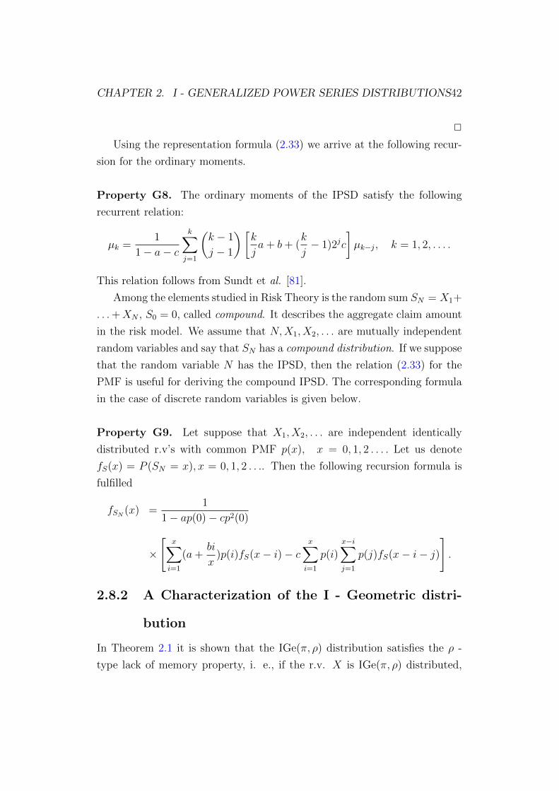
Using the representation formula (2.33) we arrive at the following recur-
sion for the ordinary moments.
Property G8. The ordinary moments of the IPSD satisfy the following
recurrent relation:
µk =1
1− a− c
k∑j=1
(k − 1
j − 1
)[k
ja+ b+ (
k
j− 1)2jc
]µk−j, k = 1, 2, . . . .
This relation follows from Sundt et al. [81].
Among the elements studied in Risk Theory is the random sum SN = X1+
. . .+XN , S0 = 0, called compound. It describes the aggregate claim amount
in the risk model. We assume that N,X1, X2, . . . are mutually independent
random variables and say that SN has a compound distribution. If we suppose
that the random variable N has the IPSD, then the relation (2.33) for the
PMF is useful for deriving the compound IPSD. The corresponding formula
in the case of discrete random variables is given below.
Property G9. Let suppose that X1, X2, . . . are independent identically
distributed r.v’s with common PMF p(x), x = 0, 1, 2 . . . . Let us denote
fS(x) = P (SN = x), x = 0, 1, 2 . . .. Then the following recursion formula is
fulfilled
fSN (x) =1
1− ap(0)− cp2(0)
×
[x∑i=1
(a+bi
x)p(i)fS(x− i)− c
x∑i=1
p(i)x−i∑j=1
p(j)fS(x− i− j)
].
2.8.2 A Characterization of the I - Geometric distri-
bution
In Theorem 2.1 it is shown that the IGe(π, ρ) distribution satisfies the ρ -
type lack of memory property, i. e., if the r.v. X is IGe(π, ρ) distributed,

CHAPTER 2. I - GENERALIZED POWER SERIES DISTRIBUTIONS43
then
P (X ≥ x+ b) =1− π(1− ρ)
1− πP (X ≥ x)P (X ≥ b), (2.36)
for all x > 0 and b > 0.
In the case of ρ = 0 the relation (2.36) coincides with the classical lack
of memory property characterizing the usual geometric distribution.
In the next proposition we will show that the property (2.36) characterizes
the IGe distribution.
Proposition 2.12 Let X be a non - negative, integer - valued random vari-
able satisfying (2.36) for any π ∈ (0, 1) and ρ ∈ [0, 1). If P (X = 0) = π,
then X is IGe(π, ρ) distributed random variable.
Proof. Let us first write (2.36) for b = 1:
P (X ≥ x+ 1) = [1− π(1− ρ)]P (X ≥ x), x > 0. (2.37)
From (2.37) by induction we get the following formula for the tail distribution
of X
P (X ≥ x+ 1) = (1− π)[1− π(1− ρ)]x, x ≥ 0. (2.38)
The relation
P (X = x) = P (X ≥ x)− P (X ≥ x+ 1)
and (2.38) give the probability mass function of the IGe(π, ρ) distribution.
2
Proposition 2.13 Let X be a non - negative, integer - valued random vari-
able satisfying
P (X = 0) = πand P (X = 1) = (1− π)π(1− ρ), (2.39)
where π ∈ (0, 1) and ρ ∈ [0, 1). Then X ∼ IGe(π, ρ) if and only if
(1− π)P (X > x+ b) = P (X > x)P (X > b), (2.40)
for every x, b = 1, 2, . . . .

CHAPTER 2. I - GENERALIZED POWER SERIES DISTRIBUTIONS44
Proof. From (2.38) we have that
P (X > x) = (1− π)(1− π(1− ρ))x, x = 1, 2, . . . ,
and then (2.40) follows. Conversely, if (2.40) holds, then
(1− π)P (X > x+ 1) = P (X > x)P (X > 1)
= P (X > x)(1− π − (1− π)π(1− ρ))
= (1− π)uP (X > x),
where u = 1− π(1− ρ). It follows that
P (X > x+ 1) = uP (X > x), x = 1, 2, . . . ,
and again (2.38) follows.
2
Theorem 2.2 Suppose that X is a r. v. with P (X ≤ x) = 1− θe−λx, x ≥
0, λ > 0, 0 < θ < 1. Let |X| = k if and only if k−1 < X ≤ k, k ≥ 0. Then
|X| has an IGe(π, ρ) distribution with π = 1− θ and ρ = (e−λ − θ)/(1− θ).
Proof. For k = 0 we have
P (|X| = 0) = P (X ≤ 0) = 1− θ.
For k ≥ 1, we have
P (|X| = k) = P (k − 1 < X ≤ k)
= θe−λ(k−1) − θe−λk
= θ(e−λ)k−1(1− e−λ).
Comparing with (??), we have π = 1− θ and (1− π)π(1− ρ) = θ(1− e−λ).It follows that
1− ρ =1− e−λ
π,
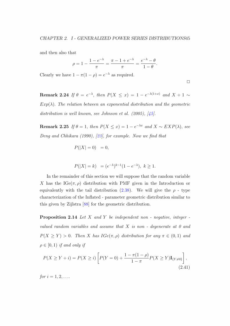
CHAPTER 2. I - GENERALIZED POWER SERIES DISTRIBUTIONS45
and then also that
ρ = 1− 1− e−λ
π=π − 1 + e−λ
π=e−λ − θ1− θ
.
Clearly we have 1− π(1− ρ) = e−λ as required.
2
Remark 2.24 If θ = e−λ, then P (X ≤ x) = 1 − e−λ(1+x) and X + 1 ∼
Exp(λ). The relation between an exponential distribution and the geometric
distribution is well known, see Johnson et al. (2005), [45].
Remark 2.25 If θ = 1, then P (X ≤ x) = 1− e−λx and X ∼ EXP (λ), see
Deng and Chhikara (1990), [23], for example. Now we find that
P (|X| = 0) = 0,
P (|X| = k) = (e−λ)k−1(1− e−λ), k ≥ 1.
In the remainder of this section we will suppose that the random variable
X has the IGe(π, ρ) distribution with PMF given in the Introduction or
equivalently with the tail distribution (2.38). We will give the ρ - type
characterization of the Inflated - parameter geometric distribution similar to
this given by Zijlstra [88] for the geometric distribution.
Proposition 2.14 Let X and Y be independent non - negative, integer -
valued random variables and assume that X is non - degenerate at 0 and
P (X ≥ Y ) > 0. Then X has IGe(π, ρ) distribution for any π ∈ (0, 1) and
ρ ∈ [0, 1) if and only if
P (X ≥ Y + i) = P (X ≥ i)
[P (Y = 0) +
1− π(1− ρ)
1− πP (X ≥ Y )IY 6=0
],
(2.41)
for i = 1, 2, . . ..

CHAPTER 2. I - GENERALIZED POWER SERIES DISTRIBUTIONS46
Proof. Let us suppose that X has the IGe distribution and P (X ≥ Y ) > 0.
Then by the relation (2.36), for every i = 1, 2, . . . we have
P (X ≥ Y + i) =∑∞
j=0 P (X ≥ j + i)P (Y = j)
= P (X ≥ i)P (Y = 0) + 1−π(1−ρ)1−π P (X ≥ i)
∑∞j=1 P (X ≥ j)P (Y = j)
= P (X ≥ i)P (Y = 0) + 1−π(1−ρ)1−π P (X ≥ i)P (X ≥ Y )IY 6=0.
This proves (2.41). We will now consider the integer - valued random variable
X, non - negative, independent of Y . Let that (2.41) be true. Obviously
∞∑j=1
P (X ≥ j+ i)P (Y = j) =1− π(1− ρ)
1− πP (X ≥ i)
∞∑j=1
P (X ≥ j)P (Y = j),
for every i = 1, 2 . . . . Rearranging the terms leads to
∞∑j=1
[P (X ≥ j + i)− 1− π(1− ρ)
1− πP (X ≥ i)P (Y ≥ j)
]P (Y = j) = 0.
The expression in the brackets equals to zero for every i = 1, 2, . . . and
P (X = 0) = π is the characterization property of the IGe(π, ρ) distribution.
2
Remark 2.26 Let us note that for every i = 1, 2, . . . . the relation (2.41) can
be rewritten in the following equivalent form
(1− π)P (X ≥ Y + i) = P (X ≥ i)P (X > Y ).
Proof. Follows immediately by combining (2.37 and (2.41).
2
In the paper of Zijlstra [88], Theorem 2 it is shown that (2.42) is a charac-
terization property of the geometric distribution. The following Proposition
gives one counter - example.
Proposition 2.15 Let X, Y and Z be independent non - negative integer -
valued random variables. Suppose X is non - degenerate, Y has the IPo(λ, ρ)

CHAPTER 2. I - GENERALIZED POWER SERIES DISTRIBUTIONS47
distribution, Z has the IPo(µ, ρ) distribution. If X has the IGe(π, ρ) distri-
bution for some π ∈ (0, 1), then
P (X ≥ Y + Z) = P (X ≥ Y )P (X ≥ Z). (2.42)
Proof. The proof follows directly from the fact that Y +Z has the IPo(λ+
µ, ρ) distribution and
P (X ≥ Y ) =1
1− π(1− ρ)
πρe−λ + (1− π)exp
(− λπ(1− ρ)
1− ρ[1− π(1− ρ)]
).
2
2.8.3 Properties of the INBD
In our first result we show how the PMF of the INB distributed r. v. Y (r)
can be obtained recursively.
Lemma 2.1 Let pr(k) = P (Y (r) = k) and pr+1(k) = P (Y (r + 1) = k). The
following relation holds:
pr+1(0) = πpr(0);
pr+1(k) = πpr(k) + (1− π)π(1− ρ)∑k−1
j=0 pr(j)uk−j−1, k = 1, 2, . . . ,
(2.43)
where u = 1− π(1− ρ).
Proof. Using the PGF, we see that Y (r + 1)d= Y (r) + Y1. It follows that
pr+1(k) =k∑j=0
pr(j)P (Y1 = k − j).
From here and using (2.2), it follows that pr+1(0) = pr(0)π and for k ≥ 1
that (2.43) holds.
2
CHAPTER 2. I - GENERALIZED POWER SERIES DISTRIBUTIONS48
Remark 2.27 If ρ = 0, (2.43) can be simplified and we find pr+1(0) = πpr(0)
and
pr+1(k) = π
k∑j=0
pr(j)(1− π)k−j, k = 1, 2, . . . .
Remark 2.28 Using the PGF of Y (r) in (2.5), we also have the following
alternative representation. We have
ψY (r)(t) =
(1− ρt1− ρ
)r (π(1− ρ)
1− (1− π(1− ρ))t
)r=
(1
1− ρ+−ρ
1− ρt
)r (π(1− ρ)
1− (1− π(1− ρ))t
)r.
If ρ < 0, the first term is the PGF of a binomial r. v. B(r) ∼ Bi(r, δ) with
parameter δ = −ρ1−ρ . The second term is the PGF of an usual negative binomial
r.v. N∗(r) with parameter π(1 − ρ). We obtain that Y (r)d= B(r) + N∗(r).
This representation can be useful for simulation purposes.
If ρ > 0, we have (1− ρ1− ρt
)rψN(r)(t) = ψN∗(r)(t).
The first term on the left hand side corresponds to the PGF of an usual
negative binomial r.v. B∗(r) with parameter ρ. Now we obtain that B∗(r) +
Y (r)d= Y ∗(r).
Since Y (r) is the sum of i.i.d. random variables, we can apply the central
limit theorem here.
Theorem 2.3 As r →∞, we have
Y (r)− rµ√rσ2
d=⇒ Z,
where µ and σ2 are given in Remark 2.5 and where Z denotes a standard
normal r. v.

CHAPTER 2. I - GENERALIZED POWER SERIES DISTRIBUTIONS49
2.9 Numerical example
In this section we will approximate the frequency data given in the column
headed ”Observed” of the Table 10.1 by using IPo(λ, ρ) and INB(π, ρ, r)
distributions. The data, taken from Daykin et al. [22] p. 52, and related
to the claims under UK comprehensive motor policies. The 421240 policies
were classified according to the number of claims in the year 1968.
Let us denote by Xn and σ2n the sampling mean and variance. Then the
average number of claims per policy is Xn = 0.13174 and σ2n = 0.13852.
In the column headed ”Poisson” of the Table 10.1 are given the cor-
responding expected values by using the usual Poisson distribution with a
parameter λ = Xn = 0.13174. The column of the Table 10.2 headed ”NB”
sets out the resulting NB approximation with parameters π = 0.951 and
r = 2.558. The last rows show the corresponding values of the Pearon’s χ2.
The value of the chi-square in the Poisson case is too high, so the insuf-
ficiency of the Poisson law for the data is evident. The reason is that the
sampling variance is greater than the sampling mean, whereas they should
be almost equal in the case of Poisson distribution. The value of χ2 in the
NB case is 9.18 which gives probability 0.05 for 5 degrees of freedom, so that
the representation is acceptable.
We will not discuss the Maximum Likelihood (ML) estimates of the pa-
rameters and their properties, but they can be calculated numerically. Here
we give the corresponding results for comparison only. The ML estimates are
obtained by a direct minimization approach of the log - likelihood following
Mickey and Britt [56]. The minimization procedure is based on derivative -
free algorithm for nonlinear least squares proposed by Ralston and Jennrich
[76].
2.9.1 IPo(λ, ρ) - case
The mean and variance of the IPo(λ, ρ) distribution are given by Remark 2.9.
Solving the corresponding system we obtain the following moment estimates

CHAPTER 2. I - GENERALIZED POWER SERIES DISTRIBUTIONS50
for the parameters ρ and λ
ρ =σ2n − Xn
σ2n + Xn
and λ =2Xn
2
σ2n + Xn
.
The same estimates can be found, for example, in Johnson et al. [45], pp.
381 - 382, where they were reported for the Polya - Aeppli distribution.
In our case we obtain the values
ρ = 0.0251 and λ = 0.12843.
The corresponding expected values are given in the column headed “IPo” of
the Table 10.1.
Table 10.1. Poisson case
k Observed Poisson IPo IPo-ML
0 370412 369246.88 370469.93 370435.301 46545 48643.57 46385.30 46447.482 3935 3204.09 4068.21 4045.883 317 140.70 296.20 291.574 28 4.63 19.14 18.615 3 0.12 1.13 1.09
≥ 6 0 0.01 0.07 0.06
Chi-square 667.52 13.60 13.61
The comparison of the expected values given in the columns headed “Pois-
son” and “IPo” shows that IPo(λ, ρ) distribution fits the observed frequen-
cies much better than the usual Poisson distribution, which has a shorter
tail than the data. The value of χ2 is 13.60 which gives probability 0.04
for 5 degrees of freedom, so the approximation by IPo(λ, ρ) distribution is
acceptable (observe that the use of the NB distribution is preferable if our
criterion is the value of the χ2 statistics).
CHAPTER 2. I - GENERALIZED POWER SERIES DISTRIBUTIONS51
Remark 2.29 We obtained a positive value for the moment estimate of the
parameter ρ. This can be interpreted in the following way: the observed num-
ber of zeros is more than it can be predicted by the usual Poisson distribution
(as it can be seen from the Table 10.1).
We obtain the following ML estimates
ρML = 0.02441 and λML = 0.12852
with χ2 = 13.61. One can see that the ML estimates of the parameters are
close to the values of the corresponding moment estimates. The correspond-
ing expected values are given in the last column of the Table 10.1.
2.9.2 INB(π, ρ, r) - case
To estimate the parameters of the INB(π, ρ, r) distribution we need addi-
tionally the third moment together with sampling mean and variance.
The mean and the variance of the r. v. X ∼ INB(π, ρ, r) are given by
Remark 2.5. From the PGF (2.5), after some algebra we obtain the following
relation for the third moment
E(X3) =r(1− π)
π
[1 + 4ρ+ ρ2 +
3(r + 1)(ρ+ 1)(1− π)
π+
(r + 1)(r + 2)(1− π)2
π2
].
The solution of the corresponding system gives the following procedure for
calculation the moment estimates of the parameters.
Step 1. The moment estimate of the parameter ρ is a solution of the fol-
lowing quadratic equation
aρ2 + bρ+ c = 0,
where
a =
(Xn +
σ2n
Xn
)(Xn +
2σ2n
Xn
)− m3 − σ2
n
Xn
,
CHAPTER 2. I - GENERALIZED POWER SERIES DISTRIBUTIONS52
b = 2− 2
(Xn +
σ2n
Xn
)(Xn +
2σ2n
Xn
)+ 2
m3
Xn
,
and
c =
(Xn +
σ2n
Xn
)(Xn +
2σ2n
Xn
)− m3 + σ2
n
Xn
with m3 being the third sample moment;
Step 2. The moment estimate for the parameter π is given by
π =
[σ2n
Xn
(1− ρ)− ρ]−1
,
where ρ is the result from Step 1;
Step 3. Finally, the moment estimate of the parameter r can be calculated
by the following formula
r =Xnπ(1− ρ)
1− π,
where ρ and π are the calculated values from Step 1 and Step 2, correspond-
ingly.
For the considered data we obtain the following moment estimates
ρ = −.03869, π = 0.88428 and r = 1.04564.
In the column headed ”INB” of the Table 10.2 are given the corresponding
estimated frequencies, when using the computed moment estimates of the
parameters. One can see that the INB(π, ρ, r) distribution fits the observed
frequencies perfectly.
Table 10.2. NB case

CHAPTER 2. I - GENERALIZED POWER SERIES DISTRIBUTIONS53
k Observed NB INB INB-ML
0 370412 370459.94 370409.99 370412.371 46545 46413.30 46553.37 46545.632 3935 4043.97 3922.17 3928.823 317 300.92 325.21 324.234 28 20.48 26.85 26.585 3 1.32 2.21 2.17
≥ 6 0 0.09 0.20 0.19
Chi-square 9.18 0.78 0.76
Remark 2.30 We calculated a negative value for the parameter ρ. This is
possible and can be interpreted in the following way: the observed number of
zeros is less than predicted by the usual NB distribution. Let us note, that in
the Poisson case we observed just the opposite situation.
We obtain the following ML estimates for the parameters
ρML = −.03670, πML = 0.88748 and rML = 1.07727,
with χ2 = 0.76. The corresponding estimated frequencies are given in the
last column of the Table 10.2.
2.10 Comments
In this chapter we derive some properties of the IGPSD in the sense of ap-
plication in Risk theory. It seams that, using these distributions as counting
distributions in the risk model, the corresponding generalization will give
good results. The advantage is in the interpretation of the additional param-
eter ρ. In general an additional parameter exhibits over - dispersion. The
distributions are suitable for modelling dependent data, which naturally ap-
pear in insurance and finance. Moreover the inflation parameter ρ may take
CHAPTER 2. I - GENERALIZED POWER SERIES DISTRIBUTIONS54
negative values, i. e.,
ρ ≥ max−1,− p0
1− p0
.
If the observed number of zeros is more than it can be predicted by the usual
GPSD, then the parameter ρ is positive. If the observed number of zeros is
less than predicted by the GPSD, the parameter ρ is negative.
The distributions, given in this chapter are published in [51], [57] and
[59]. Some additional results, related to the distributions and the Markov
chain are derived in [66].
Aoyama et. all in [7] have defined a generalization of the shifted inverse
trinomial distributions. A part of these distributions generalizes the IGPS
distributions.
Chadjiconstantinidis S. and Pitselis G. (2009) in [16], give some recursion
formulas for a class of Compound distributions. As examples they use the
IGe(π, ρ) and ILS(π, ρ) distributions.
Vinogradov in [84], Remark 2.3 gives some basic properties of the ILS(π, ρ)
distribution.
Jazi and Alamatsaz in [44] compared the ILS(π, ρ) distribution with its
mixture with respect to several stochastic orderings.
Borges et al. (2011), [14], have applied the IGPS distributions to cuta-
neous melanoma data. The number of initiated cells related to the occurrence
of a tumor is IGPS distributed and the parameter ρ is a measure of the as-
sociation between the tumor cells. The defined model is called a correlated
destructive generalized power series model (CDGPS model).
Chapter 3
Probability distributions of
order k
The distributions of order k are related to a sequence of independent trials
with success probability p. For a given fixed positive, integer number k, Feller
[31] derived the PGF of the number of trials N until the first occurrence of
k−th consecutive success
gN(s) =(1− ps)pksk
1− s+ (1− p)pksk+1. (3.1)
Philippou A., Georghiou C. and Philippou G. [72] obtained the exact
probability function corresponding to (3.1) and called it geometric distribu-
tion of order k, (Gek(p)). Philippou and Muwafi [71] show the relations
between the geometric distribution of order k and the Fibonacci numbers.
Since then many authors gave their contribution to the exact theory for the
so called discrete distributions of order k which can be called already classi-
cal. Aki and Hirano in [4] derived the distribution of the number successes
and failures until the first occurrence of k consecutive successes.
The negative binomial (NBk(r, p)) distribution of order k is the distri-
bution of the sum of r independent, identically Gek(p) distributed random
variables. Some properties of the negative binomial distribution of order k
55
CHAPTER 3. PROBABILITY DISTRIBUTIONS OF ORDER K 56
are given by Philippou in [73]. The Poisson distribution of order k, (Pok(λ)),
is a limiting distribution of a sequence of shifted NBk distributed random
variables.
The binomial distribution of order k (Bik(n, p)) was derived by Hirano
[43] and by Philippou and Makri [74]. They considered the number of success
runs of length k (N(k)n ) in n independent trials and derived the PMF. In this
definition, not every run in successes of length k gives a contribution of 1 to
N(k)n . According to this definition, N
(k)n counts the non overlapping success
runs. Ling (1988) in [54] named this distribution Type I binomial distribution
of order k. Ling defined the Type II binomial distribution of order k, which
counts the overlapping success runs.
Aki, Kuboku and Hirano [2] introduced the logarithmic series distribution
of order k (LSk(p)) as a limiting distribution of a sequence of truncated at
zero NBk distributed random variables. A good references for the distribu-
tions of order k are given in the books of Balakrishnan and Koutras [13] and
Fu and Lou [34]. Later it is proved that the discrete distributions of order k
can be represented as Compound GPSDs, (see Charalambides [17] also). Let
the random variable N has a compound distribution, i.e. N = X1 + . . .+XY ,
where X is the compounding random variable, Y is independent of X and
N = 0 in Y = 0.
Definition 3.1 If the compounding random variable X is a discrete dis-
tributed, truncated at 0 and from the right away from k + 1, the random
variable N has a distribution of order k.
The Gek(p), NBk(r, p) and the LSk(p) distributions belong to the family
of Compound GPSDs by truncated geometric compounding distribution.
In this case we suppose that the random variable X has a PMF and PGF,
given by
P (X = m) =1− ρ1− ρk
ρm−1, m = 1, 2, . . . k (3.2)
and
PX(s) =(1− ρ)s
1− ρk1− ρksk
1− ρs, (3.3)

CHAPTER 3. PROBABILITY DISTRIBUTIONS OF ORDER K 57
where k ≥ 1 is fixed integer number.
If k →∞, the truncated geometric distribution approaches to the Ge1(1−ρ) distribution, defined by (2.22) and (2.23).
In this way the Gek(p), NBk(r, p) and LSk(p) distributions converge to
the corresponding IGPSD.
The Pok(λ) distribution is obtained by discrete uniform compounding
distribution with PMF
P (X = m) =1
k, m = 1, 2, . . . k
and PGF
PX(s) =s
k
1− sk
1− s. (3.4)
As we mentioned above, the motivation of this study is related to the
risk model. In many cases the counting process in the defined model is a
compound non homogeneous Poisson process. As usual, the compounding
distribution is a discrete distribution, taking non negative integer values.
The interpretation is the following. If the insurance policies are separated in
independent groups, the number of groups has a Poisson distribution. We
suppose that the groups are homogeneous, identically distributed and the
number of policies in each of the groups has the compounding distribution.
It is not realistic if the compounding distribution takes values over all non
negative integers.
Here we define a compound Poisson distribution with compounding dis-
tribution taking values in 1, 2, ...k.
3.1 Poisson distribution of order k
In this section we present some results obtained for the Poisson distribution
of order k. Denote by Y the Pok(λ) distributed random variable. Then its
PGF is given by
PY (s) = e−λ(k−(s+s2+...+sk)), |s| ≤ 1. (3.5)
CHAPTER 3. PROBABILITY DISTRIBUTIONS OF ORDER K 58
The PMF is
P (Y = y) =∑
y1,...,yk
e−kλλy1+...+yk
y1! . . . yk!, y = 0, 1, . . . ,
where the summation is over all non - negative integers y1, y2, . . . , yk, such
that y1 + 2y2 + . . . + kyk = y. It follows from the definition that Po1(λ) ≡Po(λ). Therefore Pok(λ) is a generalized Poisson distribution.
For the random variable Y ∼ Pok(λ), we get the mean and the variance
E(Y ) = λk(k + 1)
2and V ar(Y ) = λ
k(k + 1)(2k + 1)
6.
The Fisher index of dispersion is
FI(Y ) =V ar(Y )
E(Y )= 1 +
2
3(k − 1) > 1
for k > 1.
The proof of the following Lemma follows from the PGF in (3.5).
Lemma 3.1 Let Y1, Y2, . . . , Yn be i.i.d. Poisson of order k distributed ran-
dom variables with parameters λ1, λ2, . . . , λn respectively. Then the r. v.∑nj=1 Yj is a Poisson of order k distributed with parameter λ1 +λ2 + . . .+λn.
Remark 3.1 Let Y1, Y2, . . . , Yn be independent identically Poisson distributed
of order k random variables and set Y = 1n
∑nj=1 Yj. The moment estimator
λ of λ is the unique admissible root of the equation
Y = λk(k + 1)
2.
3.2 Polya - Aeppli distribution of order k
In this section we introduce the Polya - Aeppli distribution of order k as a
compound Poisson distribution with truncated geometric compounding dis-
tribution. It is defined in [63]. The PGF is given by
PN(s) = eλ(PX(s)−1), (3.6)
CHAPTER 3. PROBABILITY DISTRIBUTIONS OF ORDER K 59
where PX(s) is the PGF of the compounding distribution in (3.3).
Definition 3.2 The probability distribution defined by the PGF (3.6) and
compounding distribution, given by (3.2) and (3.3) is called a Polya - Aeppli
distribution of order k with parameters λ > 0 and ρ ∈ [0, 1) (PAk(λ, ρ)).
The Polya - Aeppli distribution of order k belongs to the family of Com-
pound GPSD, compounded by the truncated geometric distribution. In
the next theorem we give the probability mass function. Let us denote
Z = λ(1−ρ)1−ρk .
Theorem 3.1 The probability mass function of the PAk(λ, ρ) distributed
random variable is given by:
p0 = e−λ,
pi = e−λi∑
j=1
(i− 1
j − 1
)Zj
j!ρi−j, i = 1, 2, . . . , k
pi = e−λ[i∑
j=1
(i− 1
j − 1
)Zj
j!ρi−j
−l∑
n=1
(−1)n−1 (Zρk)n
n!
i−n(k+1)∑j=0
(i− n(k + 1) + n− 1
j + n− 1
)Zj
j!ρi−n(k+1)−j],
i = l(k + 1) +m, m = 0, 1, . . . k, l = 1, 2, . . .∞.
Proof: The PMF is obtained by equating the coefficients of ti on both sides
of the Taylor expansion of the PGF.
2
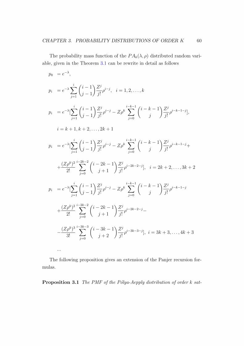
CHAPTER 3. PROBABILITY DISTRIBUTIONS OF ORDER K 60
The probability mass function of the PAk(λ, ρ) distributed random vari-
able, given in the Theorem 3.1 can be rewrite in detail as follows
p0 = e−λ,
pi = e−λi∑
j=1
(i− 1
j − 1
)Zj
j!ρi−j, i = 1, 2, . . . , k
pi = e−λ[i∑
j=1
(i− 1
j − 1
)Zj
j!ρi−j − Zρk
i−k−1∑j=0
(i− k − 1
j
)Zj
j!ρi−k−1−j],
i = k + 1, k + 2, . . . , 2k + 1
pi = e−λ[i∑
j=1
(i− 1
j − 1
)Zj
j!ρi−j − Zρk
i−k−1∑j=0
(i− k − 1
j
)Zj
j!ρi−k−1−j+
+(Zρk)2
2!
i−2k−2∑j=0
(i− 2k − 1
j + 1
)Zj
j!ρi−2k−2−j], i = 2k + 2, . . . , 3k + 2
pi = e−λ[i∑
j=1
(i− 1
j − 1
)Zj
j!ρi−j − Zρk
i−k−1∑j=0
(i− k − 1
j
)Zj
j!ρi−k−1−j
+(Zρk)2
2!
i−2k−2∑j=0
(i− 2k − 1
j + 1
)Zj
j!ρi−2k−2−j−
−(Zρk)3
3!
i−3k−3∑j=0
(i− 3k − 1
j + 2
)Zj
j!ρi−3k−3−j], i = 3k + 3, . . . , 4k + 3
...
The following proposition gives an extension of the Panjer recursion for-
mulas.
Proposition 3.1 The PMF of the Polya-Aepply distribution of order k sat-

CHAPTER 3. PROBABILITY DISTRIBUTIONS OF ORDER K 61
isfies the following recursions:
p1 = Zp0,
pi = (2ρ+ Z−2ρi
)pi−1 − (1− 2i)ρ2pi−2, i = 2, 3, . . . k
pi = (2ρ+ Z−2ρi
)pi−1 − (1− 2i)ρ2pi−2 − k+1
iZρkpi−k−1 + k
iZρk+1pi−k−2,
i = k + 1, k + 2, . . .
and p−1 = 0.
Proof. Differentiation in (3.6) leads to
(1− ρs)2P ′N(s) =1− ρ1− ρk
[1− (k + 1)ρksk + kρk+1sk+1]PN(s), (3.7)
where PN(s) =∑∞
m=0 pmsm and P ′N(s) =
∑∞m=0(m + 1)pm+1s
m. The recur-
sions are obtained by equating the coefficients of tm on both sides for fixed
m = 0, 1, 2, . . . .
2
Remark 3.2 If k → ∞, the Polya - Aeppli distribution of order k, ap-
proaches to the usual Polya - Aeppli distribution. If ρ = 0, it is a Poisson
distribution.
Remark 3.3 The mean and the variance of the Polya - Aeppli distribution
of order k are given by
EN =1 + ρ+ . . .+ ρk−2 + ρk−1 − kρk
1− ρkλ
and
V ar(N) =1 + 3ρ+ 5ρ2 + 7ρ3 + . . .+ (2k − 3)ρk−2 + (2k − 1)ρk−1 − k2ρk
1− ρkλ.

CHAPTER 3. PROBABILITY DISTRIBUTIONS OF ORDER K 62
It is easy to verify that the Fisher index of dispersion is
FI(N) =V ar(N)
E(N)> 1,
and therefore, the Polya - Aeppli distribution is overdispersed related to the
Poisson distribution.
3.3 Comments
The PMF of the Polya-Aepply distribution of order k, given in the Theorem
3.1 is published in [63]. The detailed probabilities are given in the Proceed-
ings of the ASMDA - 2007 Conference.

Chapter 4
Distributions on Markov chain
trials
We consider the time - homogeneous multi - state Markov chain Xn, n ≥ 0taking values 0, 1, 2, . . ., where the sequence X0, X1, . . . is determined by
the distribution of the initial states
P (X0 = g1) = pg1 , 0 < p0 < 1, pg1 ≥ 0, g1 = 1, 2, . . . ,∞∑g1=0
pg1 = 1,
and transition probabilities
P (Xn+1 = g2 | Xn = g1) = pg1g2 , g1, g2 = 0, 1, . . . , n = 0, 1, . . .
where
0 < p00 < 1,∞∑g2=0
pg1g2 = 1, g1 = 0, 1, . . .
and
pg1g2 ≥ 0, g1 = 1, 2, . . . , g2 = 0, 1, . . . .
We regard the value ′′0′′ as success and the remaining values ′′f ′′ as failures,
f = 1, 2, . . . .
We adopt the following classical way of counting of a ”success run of
length k”: a sequence of n outcomes of successes and failures contains as
63

CHAPTER 4. DISTRIBUTIONS ON MARKOV CHAIN TRIALS 64
many runs of length k as there are non - overlapping, uninterrupted sequence
of exactly k zeros.
4.1 Geometric distribution of order k
Let SK0 be the event
SK0 = success run of length k in the sequenceX0, X1, . . . .
Let us define the random variables
Sg1 =
1 if X0 = g1,0 if X0 6= g1,
for g1 = 0, 1, . . . and
Sg1g2 =
number of transitions of type g1 −→ g2 in the
Markov chain until the event SK0 occurs
,
for g1, g2 = 0, 1, . . ..
In this section we deal with the distribution of the random vector
S = (S0, S1, . . . , S00, S01, . . .),
under the condition that the event SK0 occurs with probability 1. To avoid
trivial complications we assume the chain to be irreducible.
Let us write fg1g2(n) for the probability that starting from state g1, the
first passage to the state g2 occurs at the nth step, g1, g2 = 0, 1, . . . . The
probability of ever visiting state g2, starting from the state g1, is fg1g2 , where
fg1g2 =∞∑n=1
fg1g2(n).
Then the condition P (SK0) = 1 is equivalent to fg10 = 1, which means that
for each g1 = 1, 2, . . . the sequences fg10(n)∞n=1 determine a proper discrete
distribution.

CHAPTER 4. DISTRIBUTIONS ON MARKOV CHAIN TRIALS 65
The following random variables are related to the defined Markov chain:
S =the total number of successesuntil the event SK0 occurs,
F =the total number of failuresuntil the event SK0 occurs
and
N = S + F.
Definition 4.1 The distribution of the random variable N is called a ge-
ometric distribution of order k for the homogeneous 0, 1, 2, . . .− valued
Markov chain.
4.1.1 The joint PGF of the random vector S
Under the given notations the following basic lemma is true
Lemma 4.1 The joint PGF of the random vector S = (S0, S1, . . . , S00, S01, . . .)
is given by
gS(t0, t1, . . . , t00, t01, . . .) = E(t0)S0(t1)S1 . . . (t00)S00(t01)S01 . . .
=A0
1− A00
(p00t00)k−1,
(4.1)
which converges at least for
(t0, t1, . . . , t00, t01, . . .) : |ti| ≤ 1 and |tij| ≤ 1, i, j = 0, 1, . . .,
where
A0 = p0t0 +∞∑g1=1
pg1tg1Fg10, (4.2)

CHAPTER 4. DISTRIBUTIONS ON MARKOV CHAIN TRIALS 66
A00 =1− (p00t00)k−1
1− p00t00
∞∑g1=1
p0g1t0g1Fg10, (4.3)
and
Fg10 = pg10tg10 +∞∑g2=1
pg1g2tg1g2pg20tg20
+∞∑g2=1
pg1g2tg1g2
∞∑g3=1
pg2g3tg2g3pg30tg30 + . . . ,
(4.4)
for g1 = 1, 2, . . . .
Proof. Let X0 = 0 and the first success is followed by k − 1 consecutive
successes. The contribution to the joint PGF gS(·) is
S0 = p0t0(p00t00)k−1.
Let the initial trial is successful, i.e. X0 = 0 and exactly r ≥ 1 subsequences
containing failures f = 1, 2, . . . are observed before the event SK0 occurs.
Then the first success ”0” is followed by no more than k− 2 consecutive suc-
cesses ”0”, before the first subsequence of failures. The second subsequence
of failures in the event SK0 (if it exists) may be preceded by no more than
k − 1 consecutive successes ”0”, followed the first subsequence of failures.
This process will be repeated till the last subsequence of failures in the event
SK0, which is followed by exactly k consecutive successes ”0”. Then, the
possible sequence of outcomes terminating in k consecutive successes ”0” and
containing exactly r subsequences of failures can be described as
0 00 . . . 0︸ ︷︷ ︸i1
ff . . . f︸ ︷︷ ︸j1
00 . . . 0︸ ︷︷ ︸i2
ff . . . f︸ ︷︷ ︸j2
. . . 00 . . . 0︸ ︷︷ ︸ir
ff . . . f︸ ︷︷ ︸jr
00 . . . 0︸ ︷︷ ︸k
,
where
0 ≤ i1 ≤ k − 2; 1 ≤ ia ≤ k − 1, a = 2, 3, . . . , r; 1 ≤ jb <∞, b = 1, 2, . . . , r.
From the Markov property of the sequences follows that the net contribution
Sr to the joint PGF gS(·) of all such sequences is
Sr = p0t0(A00)r(p00t00)k−1,

CHAPTER 4. DISTRIBUTIONS ON MARKOV CHAIN TRIALS 67
where A00 is given by (4.3);
Let X0 = f for f = 1, 2, . . . . Then the distribution of the sequence just
after the first failure is the same as the distribution after the first failure in
the above case, i.e. the contribution to the joint PGF is
Fr =∞∑g1=1
pg1tg1Fg10(A00)r−1(p00t00)k−1.
Adding all of these contributions gives
gS(t0, t1, . . . , t00, t01, . . .) = S0 +∞∑r=1
(Sr + Fr).
To see that gS(·) is a PGF, it is enough to note that for each g1 = 1, 2, . . .
the relation
Fg10(1) =∞∑n=1
fg1g2(n) = 1
is fulfilled under the assumption that P (SK0) = 1, where 1 = (1, 1, . . . , 1, . . .)
is the unit vector.
2
Remark 4.1 The same result is given in [48] in a different way. The expres-
sion (4.1) is preferable to be used since it is simpler than the corresponding
joint PGF derived in [48].
4.1.2 Number of successes in SK0.
The total number of successes S may be represented as follows
S = S0 +∞∑g1=0
Sg10.
Theorem 4.1 The distribution of S is given by the PGF
gS(t) =(1− p00t)(p00)k−1tk
1− t+ (1− p00)(p00)k−1tk. (4.5)

CHAPTER 4. DISTRIBUTIONS ON MARKOV CHAIN TRIALS 68
Proof. The relation (4.5) is obtained from (4.1) by substituting
t0 = tg10 = t, g1 = 0, 1, . . .
and
tg1 = 1, g1 = 1, 2, . . . , tg1g2 = 1, g1 = 0, 1, . . . and g2 = 1, 2, . . . .
2
Remark 4.2 The presentation (4.5) is the PGF of the shifted geometric
distribution of order k−1 and its support begins with k. The probability mass
function of S is given by
P (S = m) =∑
m1,...mk−1
(m1 + . . .+mk−1
m1, . . . ,mk−1
)(p00)m
(q00
p00
)m1+...+mk−1
,
for m = k, k + 1, . . . , where q00 = 1 − p00 and the summation is over all
nonnegative integers m1,m2, . . .mk−1, such that
m1 + 2m2 + . . .+ (k − 1)mk−1 = m− k + 1.
It is somewhat surprising to note from (4.5) that the distribution of S de-
pends only on p00 and it is unaffected by the values pg1 and pg1g1 , g1 = 0, 1, . . .
and g2 = 1, 2, . . . . Hence we can treat a homogeneous multi-state Markov
chain as the independent, identically distributed sequence. This conclusion
was obtained by Aki and Hirano [4] for the 0, 1− valued homogeneous
Markov chain (their Theorem 3.2, p.199).
4.1.3 Number of failures
The total number of failures F may be represented as follows
F =∞∑g1=1
Sg1 +∞∑g1=0
∞∑g2=1
Sg1g2 .
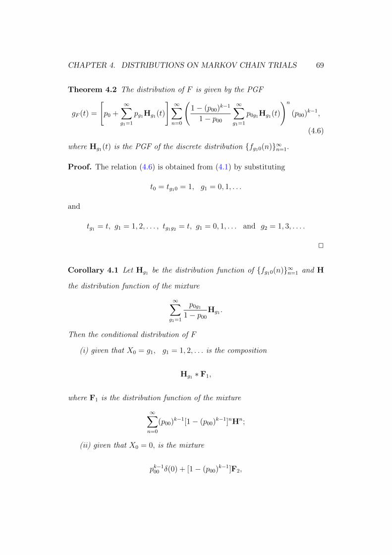
CHAPTER 4. DISTRIBUTIONS ON MARKOV CHAIN TRIALS 69
Theorem 4.2 The distribution of F is given by the PGF
gF (t) =
[p0 +
∞∑g1=1
pg1Hg1(t)
]∞∑n=0
(1− (p00)k−1
1− p00
∞∑g1=1
p0g1Hg1(t)
)n
(p00)k−1,
(4.6)
where Hg1(t) is the PGF of the discrete distribution fg10(n)∞n=1.
Proof. The relation (4.6) is obtained from (4.1) by substituting
t0 = tg10 = 1, g1 = 0, 1, . . .
and
tg1 = t, g1 = 1, 2, . . . , tg1g2 = t, g1 = 0, 1, . . . and g2 = 1, 3, . . . .
2
Corollary 4.1 Let Hg1 be the distribution function of fg10(n)∞n=1 and H
the distribution function of the mixture
∞∑g1=1
p0g1
1− p00
Hg1 .
Then the conditional distribution of F
(i) given that X0 = g1, g1 = 1, 2, . . . is the composition
Hg1 ∗ F1,
where F1 is the distribution function of the mixture
∞∑n=0
(p00)k−1[1− (p00)k−1]nHn;
(ii) given that X0 = 0, is the mixture
pk−100 δ(0) + [1− (p00)k−1]F2,
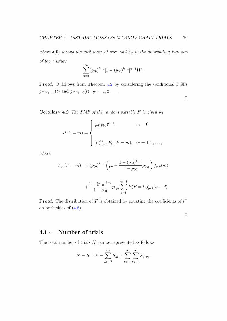
CHAPTER 4. DISTRIBUTIONS ON MARKOV CHAIN TRIALS 70
where δ(0) means the unit mass at zero and F2 is the distribution function
of the mixture∞∑n=1
(p00)k−1[1− (p00)k−1]n−1Hn.
Proof. It follows from Theorem 4.2 by considering the conditional PGFs
gF |X0=g1(t) and gF |X0=0(t), g1 = 1, 2, . . . .
2
Corollary 4.2 The PMF of the random variable F is given by
P (F = m) =
p0(p00)k−1, m = 0
∑∞g1=1 Pg1(F = m), m = 1, 2, . . . ,
where
Pg1(F = m) = (p00)k−1
(p0 +
1− (p00)k−1
1− p00
p0g1
)fg10(m)
+1− (p00)k−1
1− p00
p0g1
m−1∑i=1
P (F = i)fg10(m− i).
Proof. The distribution of F is obtained by equating the coefficients of tm
on both sides of (4.6).
2
4.1.4 Number of trials
The total number of trials N can be represented as follows
N = S + F =∞∑g1=0
Sg1 +∞∑g1=0
∞∑g2=0
Sg1g2 .

CHAPTER 4. DISTRIBUTIONS ON MARKOV CHAIN TRIALS 71
Theorem 4.3 The distribution of N is given by the PGF
gN(t) =
p0 +∞∑g1=1
pg1Hg1(t)
1− 1− (p00t)k−1
1− p00t
∞∑g1=1
p0g1tHg1(t)
(p00)k−1tk, (4.7)
where Hg1(t) is the PGF of the discrete distribution fg10(n)∞n=1.
Proof. The relation (4.7) is obtained from (4.1) by substituting
tg1 = tg1g2 = t, g1, g2 = 0, 1, . . . .
2
This leads to the second definition of the geometric distributions of order
k.
Definition 4.2 The distribution with PGF given by (4.7) is called a geomet-
ric distribution of order k related to homogeneous multi-state Markov chain.
Corollary 4.3 The PMF of the random variable N is given by
P (N = k) = p0(p00)k−1
P (N = k + 1) = (p00)k−1
∞∑g1=1
pg1pg10
P (N = m) = (p00)k−1
∞∑g1=1
pg1pf10(m− k)
+∑
i+n+j=m−1
P (N = i)(p00)n∞∑g1=1
p0g1fg10(j), m = k + 2, k + 3, . . . ,
where the summation is over the nonnegative integers i, n and j such that
j ≥ k, 0 ≤ n ≤ k − 2 and j ≥ 1.

CHAPTER 4. DISTRIBUTIONS ON MARKOV CHAIN TRIALS 72
Proof. The distribution of N is obtained by equating the coefficients of tm
on both sides in (4.7), m ≥ k.
2
Remark 4.3 For two - state Markov chain, the distribution of N and its
PGF was outlined by Aki and Hirano [3] where it is understood that X0 is
not counted in measuring the length of the run (Corollary on p. 469).
Corollary 4.4 The expected number of trials in SK0 is given by
EN = 1 +∞∑g1=1
pg1E(g1) +(p00)1−k − 1
1− p00
(∞∑g1=1
p0g1E(g1) + 1
), (4.8)
where for g1 = 1, 2, . . .
E(g1) =∞∑i=1
ifg10(i).
Proof. The expression (4.8) is obtained after simplification of the relation
EN =d
dtgN(t)
∣∣∣∣t=1
.
2
Example 4.1 (Random walk model). Let us consider the motion of a par-
ticle which moves in discrete jumps with certain probabilities from point to
point. We imagine the particle starts at the point x = i with probability pi
on the x - axis, i = 1, 2, . . . . For each subsequent time it moves one unit
to the right, one unit to the left or remains where it is with probabilities
0 < pi,i+1 < 1, 0 < pi,i−1 < 1 or pii, respectively, where
pi,i−1 + pii + pi,i+1 = 1, i = 1, 2, . . . .

CHAPTER 4. DISTRIBUTIONS ON MARKOV CHAIN TRIALS 73
If it happens that the particle starts at the point x = 0 with probability p0 ∈
(0, 1), it moves at the next time only one unit to the right or remains where
it is with probabilities p01 or p00 ∈ (0, 1), respectively where
p00 + p01 = 1.
The same rule is fulfilled if in some time the particle is at the point x = 0
on the x - axis.
The considered random walk model can be described by a homogeneous
Markov chain with the following transition probability matrix
p00 p01 0 0 0 · · ·
p10 p11 p12 0 0 · · ·
0 p21 p22 p23 0 · · ·
0 0 p32 p33 p34 · · ·...
......
......
...
Let us note that the PGF gN(t) in (4.7) is unaffected by the zero-values of
the above matrix. In particular, this means that Hg1(t) =∑∞
i=g1fg10(i)ti for
g1 = 1, 2, . . . .
Example 4.2 (Urn model). Suppose that there are urns numbered by 0, 1, 2, . . . .
Each urn contains balls numbered by 0, 1, 2, . . . . The content of each urn
remains constant (each sampled ball is returned to the urn). Let pg1 de-
note the probability that the initial drawing will be from the urn with number
g1, g1 = 0, 1, 2, . . . ,∑∞
g1=0 pg1 = 1. Let pg1g2 be the probability that a ball
bearing the number g2 is drawn from the g1th urn,∑∞
g2=0 pg1g2 = 1. Then
the next ball will be drawn from the urn numbered by g2, g2 = 0, 1, 2, . . . .
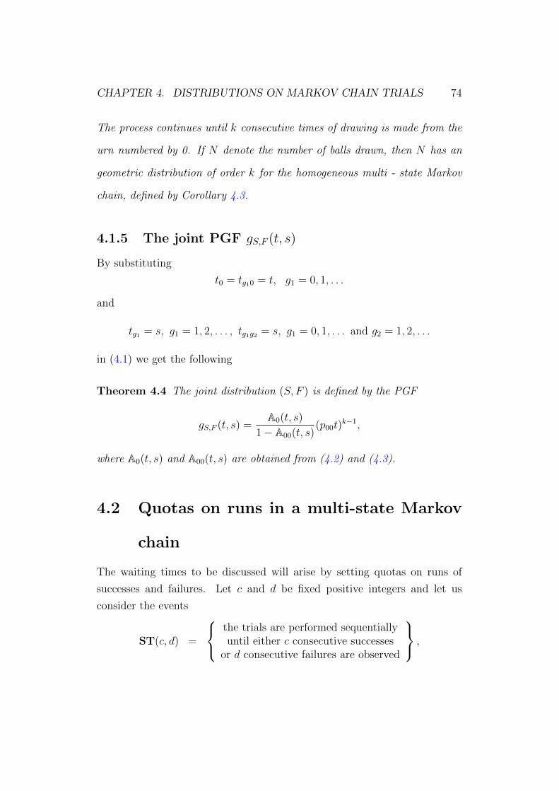
CHAPTER 4. DISTRIBUTIONS ON MARKOV CHAIN TRIALS 74
The process continues until k consecutive times of drawing is made from the
urn numbered by 0. If N denote the number of balls drawn, then N has an
geometric distribution of order k for the homogeneous multi - state Markov
chain, defined by Corollary 4.3.
4.1.5 The joint PGF gS,F (t, s)
By substituting
t0 = tg10 = t, g1 = 0, 1, . . .
and
tg1 = s, g1 = 1, 2, . . . , tg1g2 = s, g1 = 0, 1, . . . and g2 = 1, 2, . . .
in (4.1) we get the following
Theorem 4.4 The joint distribution (S, F ) is defined by the PGF
gS,F (t, s) =A0(t, s)
1− A00(t, s)(p00t)
k−1,
where A0(t, s) and A00(t, s) are obtained from (4.2) and (4.3).
4.2 Quotas on runs in a multi-state Markov
chain
The waiting times to be discussed will arise by setting quotas on runs of
successes and failures. Let c and d be fixed positive integers and let us
consider the events
ST(c, d) =
the trials are performed sequentiallyuntil either c consecutive successes
or d consecutive failures are observed
,

CHAPTER 4. DISTRIBUTIONS ON MARKOV CHAIN TRIALS 75
ST1(c) =
the trials are performed sequentially
until c consecutive successes are observed
,
ST2(d) =
the trials are performed sequentially
until d consecutive failures are observed
,
and
LT(c, d) =
the trials are performed sequentially upon
completion of both a run of c successesand a run of d failures
.
It is clear that the sooner occurring event ST(c, d) and the later occurring
event LT(c, d) between ST1(c) and ST2(d) are determined by the relations
ST(c, d) = ST1(c) ∪ ST2(d) (4.9)
and
LT(c, d) = ST1(c) ∩ ST2(d). (4.10)
In this section we extend to the present homogeneous Markov chain the
waiting time problems related with the events ST(c, d) and LT(c, d). These
events are studied by Balasubramanian et al. [12] for Markov correlated
Bernoulli trials, where the review of literature is given.
Similar results for two - state homogeneous Markov chain are obtained
by Aki and Hirano ([3]) and Uchida and Aki [83]. The distribution theory
of runs in different Markov fashions is developed by many authors. Some
important references are Aki et al. [1], Balakrishnan [8], Doi and Yamamoto
[27], Ebneshahrashoob and Sobel [29], Fu and Koutras [33], Koutras [52]. In
Balakrishnan et al. [9], Balakrishnan and Chan [10] and Balakrishnan et al.
[11] the start - up demonstration tests are discussed as an application of the
distributions of order k. It is a demonstration of the starting - up reliability
of some equipment.
4.2.1 Sooner waiting time problems
We start with the distribution of the random vector
S = (S0, S1, . . . , S00, S01, . . .),

CHAPTER 4. DISTRIBUTIONS ON MARKOV CHAIN TRIALS 76
under the condition that the event ST(c, d) occurs with probability 1. Under
the given notations the following basic lemma is true.
Lemma 4.2 The joint probability generating function of the random vector
S related with the event ST(c, d) is given by
gS(t0, t1, . . . , t00, t01, . . .) = E(t0)S0(t1)S1 . . . (t00)S00(t01)S01 . . .
=∞∑g1=1
pg1tg1F(d)g1
+A0C00
1− A00
(4.11)
which converges at least for
(t0, t1, . . . , t00, t01, . . .) : |ti| ≤ 1 and |tij| ≤ 1, i, j = 0, 1, . . .
and
A0 = p0t0 +∞∑g1=1
pg1tg1F(d−1)g10 , (4.12)
A00 =1− (p00t00)c−1
1− p00t00
∞∑g1=1
p0g1t0g1F(d−1)g10 , (4.13)
C00 = (p00t00)c−1 +1− (p00t00)c−1
1− p00t00
∞∑g1=1
p0g1t0g1F(d)g1,
where for g1 = 1, 2, . . . and d > 1
F (d)g1
=∞∑g2=1
pg1g2tg1g2 . . .∞∑gd=1
pgd−1gdtgd−1gd , (4.14)
F(d−1)g10 = pg10tg10 +
∞∑g2=1
pg1g2tg1g2pg20tg20 + . . .
+∞∑g2=1
pg1g2tg1g2 . . .∞∑
gd−1=1
pgd−2gd−1tgd−2gd−1
pgd−10tgd−10.
(4.15)
If d = 1 the expressions (4.14) and (4.15) are equal to
F (d)g1
= 1 and F(d−1)g10 = 0.
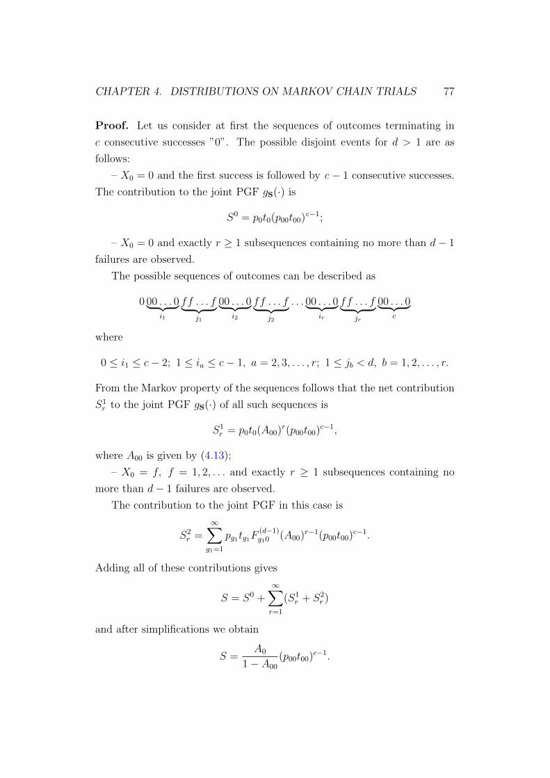
CHAPTER 4. DISTRIBUTIONS ON MARKOV CHAIN TRIALS 77
Proof. Let us consider at first the sequences of outcomes terminating in
c consecutive successes ”0”. The possible disjoint events for d > 1 are as
follows:
– X0 = 0 and the first success is followed by c − 1 consecutive successes.
The contribution to the joint PGF gS(·) is
S0 = p0t0(p00t00)c−1;
– X0 = 0 and exactly r ≥ 1 subsequences containing no more than d− 1
failures are observed.
The possible sequences of outcomes can be described as
0 00 . . . 0︸ ︷︷ ︸i1
ff . . . f︸ ︷︷ ︸j1
00 . . . 0︸ ︷︷ ︸i2
ff . . . f︸ ︷︷ ︸j2
. . . 00 . . . 0︸ ︷︷ ︸ir
ff . . . f︸ ︷︷ ︸jr
00 . . . 0︸ ︷︷ ︸c
where
0 ≤ i1 ≤ c− 2; 1 ≤ ia ≤ c− 1, a = 2, 3, . . . , r; 1 ≤ jb < d, b = 1, 2, . . . , r.
From the Markov property of the sequences follows that the net contribution
S1r to the joint PGF gS(·) of all such sequences is
S1r = p0t0(A00)r(p00t00)c−1,
where A00 is given by (4.13);
– X0 = f, f = 1, 2, . . . and exactly r ≥ 1 subsequences containing no
more than d− 1 failures are observed.
The contribution to the joint PGF in this case is
S2r =
∞∑g1=1
pg1tg1F(d−1)g10 (A00)r−1(p00t00)c−1.
Adding all of these contributions gives
S = S0 +∞∑r=1
(S1r + S2
r )
and after simplifications we obtain
S =A0
1− A00
(p00t00)c−1.

CHAPTER 4. DISTRIBUTIONS ON MARKOV CHAIN TRIALS 78
Let us consider the sequences of outcomes terminating in d consecutive
failures f = 1, 2, . . . when d > 1.
Let X0 = f and the first failure is followed by d− 1 consecutive failures.
The contribution to the joint PGF in this case is
F1 =∞∑g1=1
pg1tg1F(d)g1.
Next, the contribution to the joint PGF, when the initial trial is successful
followed by no more than c− 1 consecutive successes preceded the sequence
of d consecutive failures, is given by
F2 = p0t01− (p00t00)c−1
1− p00t00
∞∑g1=1
p0g1t0g1F(d)g1.
The corresponding contributions F 1r and F 2
r from the sequences ending
with d consecutive failures, containing exactly r ≥ 1 subsequences of failures
and beginning with a success or a failure are
F 1r = p0t0(A00)r
1− (p00t00)c−1
1− p00t00
∞∑g1=1
p0g1t0g1F(d)g1
and
F 2r =
∞∑g1=1
pg1tg1F(d−1)g10 (A00)r−1 1− (p00t00)c−1
1− p00t00
∞∑g1=1
p0g1t0g1F(d)g1,
where A00, F(d)g1 and F
(d−1)g10 are given by (4.13), (4.14) and (4.15). Adding of
all of these contributions gives
F = F1 + F2 +∞∑r=1
(F 1r + F 2
r ),
i.e.
F =∞∑g1=1
pg1tg1F(d)g1
+A0
1− A00
[C00 − (p00t00)c−1
].
The joint PGF gS(·) given by (4.11) is obtained by
gS(t0, t1, . . . , t00, t01, . . .) = S + F.

CHAPTER 4. DISTRIBUTIONS ON MARKOV CHAIN TRIALS 79
At the end, if d = 1, the joint PGF is given by the following expression
∞∑g1=1
pg1tg1 + p0t0
[(p00t00)c−1 +
1− (p00t00)c−1
1− p00t00
∞∑g1=1
p0g1t0g1
],
i.e. one can substitute F(d)g1 = 1 and F
(d−1)g10 = 0 in (4.11).
To see that gS(·) is a PGF, let us put in (4.11) all arguments equal to
1 and 1 = (1, 1, . . . , 1, 1, . . .) be the corresponding unit vector. Then the
following relations
F(d−1)g10 (1) =
d−1∑i=1
fg10(i) = 1− F (d)g1
(1)
and
1− A00(1) = C00(1),
are true. Here fg10(i) means the probability that first visit to state 0 from
some failure state occurs in exactly i steps, i = 1, 2, . . . , d− 1.
2
Remark 4.4 Lemma 4.2 is true under the condition that P (ST(c, d)) = 1,
which is always fulfilled for irreducible Markov chains with persistent set of
states.
If the states of the chain are transient, for the realization of the event
ST(c, d) with probability 1, it is necessary all possible sequences of outcomes
between the first and the last observed successive state ′′0′′ in the event
ST(c, d) to belong to the same state, say P0, of transient states.
Let X0 = 0 and the sequences of outcomes terminate in d consecutive
transient failure states. Beginning from some of the last d failure states it
is possible the elements of the following subsequence to belong to the upper
(according P0) sets of states.
Let the chain starts with a failure state. Then some subsequence of
consecutive failure states, followed the initial state of the chain and preceding
the first successive state, may belong to the lower (according P0) set of
transient states.

CHAPTER 4. DISTRIBUTIONS ON MARKOV CHAIN TRIALS 80
Remark 4.5 If the homogeneous Markov chain has two states from (4.11)
one can obtain the corresponding joint PGF given by Balasubramanian et
al. ([12]) in their Proposition 1. Lemma 4.2 generalizes the PGF given in
Theorem 1 by Aki and Hirano ([3]), where it is understood that X0 is not
counted in measuring the length of the run in two - state Markov chain.
Remark 4.6 By substituting in (4.11)
t0 = tg10 = s, g1 = 0, 1, . . .
and
tg1 = t, g1 = 1, 2, . . . ; tg1g2 = t, g1 = 0, 1, . . . and g2 = 1, 2, . . .
we obtain the joint PGF
gS,F (s, t) =∞∑x=0
∞∑y=0
P (X = x, F = y)sxty (4.16)
of the random vector (S, F ), where S and F are the numbers of successes
and failures in the event ST(c, d), respectively. From (4.16) it is possible to
calculate the Cov(S, F ).
Let us denote by
a1(j) =∞∑g1=1
pg1fg10(j), j = 1, 2, . . . , d− 1,
a0(j) =∞∑g1=1
p0g1fg10(j), j = 1, 2, . . . , d− 1,
a1(d) =∞∑g1=1
pg1F(d)g1
(1)

CHAPTER 4. DISTRIBUTIONS ON MARKOV CHAIN TRIALS 81
and
a0(d) =∞∑g1=1
p0g1F(d)g1
(1),
where fg10(j) are the probabilities defined in the proof of Theorem 4.2 and 1
means the corresponding unit vector.
From (4.16) one can obtain the following exact join distribution of the
random vector (S, F ) :
P (S = x, F = y) = 0 for x < c and y < d;
P (S = c, F = 0) = p0(p00)c−1;
P (S = 0, F = d) = a1(d);
P (S = c, F = d) = 0;
P (S = c+ i, F = 0) = 0 for i = 1, 2, . . . ;
P (S = 0, F = d+ j) = 0 for j = 1, 2, . . . ;
P (S = c, F = j) = a1(j)(p00)c−1 for j = 1, 2, . . . , d− 1;
P (S = i, F = d) = p0(p00)i−1a0(d) for i = 1, 2, . . . , c− 1,
P (S = i, F = d+ j) = (p00)i−1[a1(j)a0(d)− a0(j)a1(d)]
+i∑
m=1
j∑n=1
(p00)m−1a0(n)P (S = i−m,F = d+ j − n)
for i = 1, 2, . . . , c− 1 and j = 1, 2, . . . , d− 1.
The remaining joint probabilities for x = c, y = d+ 1, d+ 2, . . . , 2d− 1 and
x ≥ c+ 1, y ≥ 2d, are given recursively by the following relation
P (S = x, F = y) =c−1∑m=1
d−1∑n=1
(p00)m−1a0(n)P (S = x−m,F = y − n).
From (4.16) can be obtained the marginal PGF’s gS(s), gF (t) and gN(u)
of the total number of successes S, the total number of failures F and the
total number of trials N in the event ST(c, d), respectively, as well as the
corresponding probability mass functions and expected waiting times.
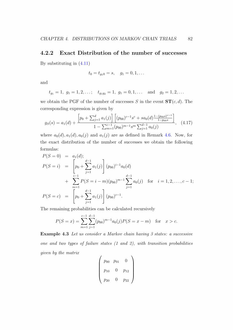
CHAPTER 4. DISTRIBUTIONS ON MARKOV CHAIN TRIALS 82
4.2.2 Exact Distribution of the number of successes
By substituting in (4.11)
t0 = tg10 = s, g1 = 0, 1, . . .
and
tg1 = 1, g1 = 1, 2, . . . ; tg1g2 = 1, g1 = 0, 1, . . . and g2 = 1, 2, . . .
we obtain the PGF of the number of successes S in the event ST(c, d). The
corresponding expression is given by
gS(s) = a1(d) +
[p0 +
∑dj=1 a1(j)
] [(p00)c−1sc + sa0(d)1−(p00s)c−1
1−p00s
]1−
∑c−1m=1(p00)m−1sm
∑d−1j=1 a0(j)
, (4.17)
where a0(d), a1(d), a0(j) and a1(j) are as defined in Remark 4.6. Now, for
the exact distribution of the number of successes we obtain the following
formulas:
P (S = 0) = a1(d);
P (S = i) =
[p0 +
d−1∑j=1
a1(j)
](p00)i−1a0(d)
+i−1∑m=1
P (S = i−m)(p00)m−1
d−1∑j=1
a0(j) for i = 1, 2, . . . , c− 1;
P (S = c) =
[p0 +
d−1∑j=1
a1(j)
](p00)c−1.
The remaining probabilities can be calculated recursively
P (S = x) =c−1∑m=1
d−1∑j=1
(p00)m−1a0(j)P (S = x−m) for x > c.
Example 4.3 Let us consider a Markov chain having 3 states: a successive
one and two types of failure states (1 and 2), with transition probabilities
given by the matrix p00 p01 0
p10 0 p12
p20 0 p22

CHAPTER 4. DISTRIBUTIONS ON MARKOV CHAIN TRIALS 83
and p0 + p1 = 1.
This matrix corresponds to the single corrective action model for a start-
up demonstration test under the Markovian dependence structure studied by
Balakrishnan et al. [11]. We slightly simplify the model accepting the same
probability
p00 = P (success | previous trial is successive).
In a single corrective action model, one corrective action of the equipment is
allowed (failure of type 1), resulting in a change in the probability of success
just after a failure, until specified number of consecutive start-ups, say c, are
observed. This means that just after the first failure the system changes his
behavior. So, it is impossible the to begin with a failure of the second type.
Because of this p2 = 0.
Under these assumptions, one can obtain from (4.17), with d → ∞, the
PGF given in Theorem 2.1 in [11].
Let us substitute d = 3. This means that under the corrective action
model, the start-ups are terminated upon the c - th consecutive successive
state of the equipment or just after the third observed consecutive failure.
In this case, we have the following simple expressions
a0(1) = p01p10;
a0(2) = p01p12p20;
a0(3) = p01p12p22;
a1(1) = p1p10;
a1(2) = p1p12p20;
a1(3) = p1p12p22,

CHAPTER 4. DISTRIBUTIONS ON MARKOV CHAIN TRIALS 84
which are used in calculating the probabilities P (S = x), x = 0, 1, . . . .
Remark 4.7 Letting d → ∞ in the event ST(c, d) yields the event SK0.
Then from (4.16) we obtain the joint PGF g(c,∞) until a run of c consecutive
successes in a multi - state Markov chain is observed, given by
g(c,∞) =A0
1− A00
(p00t00)c−1, (4.18)
where A0 and A00 are given by (4.2) and (4.3).
Let us note that in this limiting case, the relation (4.18) is true only for
irreducible Markov chain with persistent set of states.
4.2.3 Exact distribution of the number of failures
By analogy with the previous subsection, let us substitute
t0 = tg10 = 1, g1 = 0, 1, . . .
and
tg1 = t, g1 = 1, 2, . . . , tg1g2 = t, g1 = 0, 1, . . . and g2 = 1, 2, . . .
As a result, from (4.11) one can obtain the PGF gF (t) of the total number
F of failures in the event ST(c, d)
gF (t) = a1(d)td +
[p0 +
∑d−1j=1 a1(j)tj
] [(p00)c−1 + a0(d)1−(p00)c−1
1−p00 td]
1− 1−(p00)c−1
1−p00
∑d−1j=1 a0(j)tj
,
where the expressions for a0(d), a1(d), a0(j) and a1(j) are given in Remark
4.6. The probability mass function of the total number of failures is given

CHAPTER 4. DISTRIBUTIONS ON MARKOV CHAIN TRIALS 85
by the following relations
P (F = 0) = p0(p00)c−1;
P (F = j) =
[a1(j) + p0
1− (p00)c−1
1− p00
a0(j)
](p00)c−1 for j = 1, 2, . . . , d− 1;
P (F = d) = a1(d) + p01− (p00)c−1
1− p00
a0(d);
P (F = d+ j) =1− (p00)c−1
1− p00
[a1(j)a0(d) + p0
1− (p00)c−1
1− p00
a0(j)a0(d)
+d−1∑
k=1, k 6=j
P (F = d+ j − k)a0(k)
]for j = 1, 2, . . . , d− 1.
The remaining probabilities can be calculated recursively
P (F = y) =1− (p00)c−1
1− p00
d−1∑j=1
a0(j)P (F = y − j) for y ≥ 2d.
Example 4.4 Let us consider a random walk model over the non-negative
integers determined by the following transition matrix
p00 p01 0 0 0 · · ·
p10 p11 p12 0 0 · · ·
0 p21 p22 p23 0 · · ·
0 0 p32 p33 p34 · · ·...
......
......
...
and p0 +p1 +. . . = 1. If we substitute d = 3, we have the following expressions
a0(1) = p01p10;
a0(2) = p01p11p10;
a0(3) = p01[p11(p11 + p12) + p12];
a1(1) = p1p10;
a1(2) = p1p11p10;
a1(3) = 1 + p1[p11(p11 + p12) + p12 − 1] + p2p21(p11 + p12 − 1)− p0

CHAPTER 4. DISTRIBUTIONS ON MARKOV CHAIN TRIALS 86
and one can calculate the probabilities P (F = y), y ≥ 0.
Remark 4.8 Letting c→∞ in the event ST(c, d) yields the event ST2(d).
From (4.16) we obtain the joint PGF g(∞, d) until a run of d consecutive
failures in a multi - state Markov chain is observed, given by
g(∞, d) =∞∑g1=1
[pg1tg1 +
p0t0 +∑∞
l=1 plt1F(d−1)l0
1− p00t00
∑∞l=1 p0lt0lF
(d−1)l0
p0g1t0g1
]F (d)g1, (4.19)
where F(d)g1 and F
(d−1)g10 are the expressions (4.14) and (4.15), respectively.
As in the previous case, (4.19) is true only for irreducible Markov chains
with persistent set of states.
4.2.4 Later waiting time problems
The latter case in this section arises when stopping the experiment upon
completion of both a run of c successes and a run of d failures in a multi
state Markov chain, i.e. we deal with the event LT(c, d) and associated
random variables
S1g1g2
=
number of transitions of type g1 −→ g2 in theMarkov chain until the event LT(c, d) occurs
,
for g1, g2 = 0, 1, . . . under condition that P (LT(c, d)) = 1.
The joint PGF gLT(c, d) related with the random vector S can be ob-
tained from the results derived in Section 2 because of duality noticed by
Balasubramanian et al. [12] and based on the relations (4.9) and (4.10).
If we denote by gST(c, d) the joint PGF given by (4.11), then the joint
PGF gLT(c, d) is determined by
gLT(c, d) = g(c,∞) + g(∞, d)− gST(c, d), (4.20)
where g(c,∞) and g(∞, d) are expressions (4.18) and (4.19). Similar rela-
tionships hold for any marginal PGF’s.

CHAPTER 4. DISTRIBUTIONS ON MARKOV CHAIN TRIALS 87
Remark 4.9 From (4.11) one can obtain the corresponding joint PGF, given
by Aki and Hirano [3] in their Theorem 2 where it is understood that X0 is
not counted in measuring the length of the run in two-state Markov chain.
Remark 4.10 The condition P (LT(c, d)) = 1 implies that the joint PGF
determined by (4.20) have to be modified as follows
gLT(c, d, c1, d1) = g(c, d1) + g(c1, d)− gST(c, d),
where c ≤ c1 <∞ and d ≤ d1 <∞ with c1 and d1 being the maximal possible
length of runs of successes and failures within the set P0, defined by Remark
4.4.
4.3 Run and frequency Quotas in a multi-
state Markov cnain
For Markov correlated Bernoulli trials Balasubramanian et al. [12] studied
the waiting time problems related with the events
RF(c, d) =
the trials are performed sequentiallyuntil either c consecutive successesor d failures in total are observed
and
FR(c, d) =
the trials are performed sequentially
until either c successes in totalor d consecutive failures are observed
where c and d are fixed positive integers.
Some waiting time problems related with quotas on runs of successes and
failures are studied by Aki et al. [1], Balakrishnan et al. [11], Doi and
Yamamoto [27], Fu and Koutras [33], Koutras [52].

CHAPTER 4. DISTRIBUTIONS ON MARKOV CHAIN TRIALS 88
Let us define the random variables
Sg1 =
1 if X0 = g1,0 if X0 6= g1,
for g1 = 0, 1, . . . ,
S1g1g2
=
number of transitions of type g1 −→ g2
in the Markov chain until the eventRF(c, d) occurs
and
S2g1g2
=
number of transitions of type g1 −→ g2
in the Markov chain until the eventFR(c, d) occurs
,
for g1, g2 = 0, 1, . . . .
Here we are interested on joint probability generating functions (PGF)
related with the random vectors
Si = (S0, S1, . . . , Si00, S
i01, . . .), i = 1, 2,
under condition that the events FR(c, d) and RF(c, d) occur with probability
1. Interpretation of the results is given in terms of start - up demonstration
tests.
4.3.1 Run Quota on successes and frequency Quota on
failures
In this section we will study the waiting time problems, related with the
event RF(c, d). The basic result is given by the following lemma.
Lemma 4.3 The joint PGF of the random vector
S1 = (S0, S1, . . . , S100, S
101, . . .)

CHAPTER 4. DISTRIBUTIONS ON MARKOV CHAIN TRIALS 89
related with the event RF(c, d) is given by
gS1(t0, t1, . . . , t00, t01, . . .) = gS1(c, d) = E(t0)S0(t1)S1 . . . (t00)S100(t01)S
101 . . .
= p0t0(p00t00)c−1 +∑∞
g1=1Ag1Bg1 ,
(4.21)
which converges at least for
(t0, t1, . . . , t00, t01, . . .) : |ti| ≤ 1 and |tij| ≤ 1, i, j = 0, 1, . . .
where for d > 1
Ag1 = p0t01− (p00t00)c−1
1− p00t00
p0g1t0g1 + pg1tg1 , (4.22)
Bg1 = B(d)g1
+B(d−1)g10 (p00t00)c−1, (4.23)
B(d)g1
=∞∑g2=1
Bg1g2
∞∑g3=1
Bg2g3 . . .∞∑gd=1
Bgd−1gd , (4.24)
B(d−1)g10 = pg10tg10 +
∞∑g2=1
Bg1g2pg20tg20 + . . .
+∞∑g2=1
Bg1g2
∞∑g3=1
Bg2g3 . . .∞∑
gd−1=1
Bgd−2gd−1pgd−10tgd−10,
(4.25)
for g1 = 1, 2, . . . and
Bgigj = pgi0tgi01− (p00t00)c−1
1− p00t00
p0gj t0gj + pgigj tgigj (4.26)
for i, j = 1, 2, . . . .
If d = 1, B(d)g1 = 1 and B
(d−1)g10 = 0.
Proof. The joint PGF given by (4.21) is obtained in a usual way by consid-
ering all possible sequences of outcomes beginning with a success or failure
and terminating with c consecutive successes or until d failures in total are
observed.
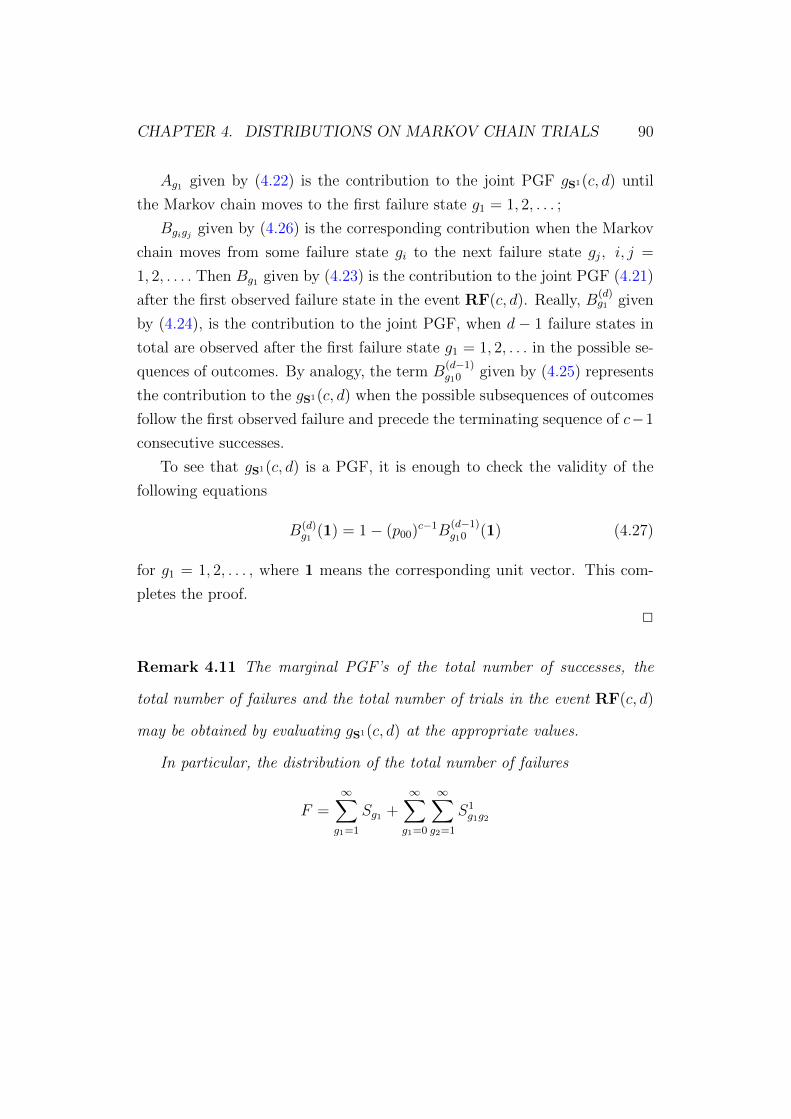
CHAPTER 4. DISTRIBUTIONS ON MARKOV CHAIN TRIALS 90
Ag1 given by (4.22) is the contribution to the joint PGF gS1(c, d) until
the Markov chain moves to the first failure state g1 = 1, 2, . . . ;
Bgigj given by (4.26) is the corresponding contribution when the Markov
chain moves from some failure state gi to the next failure state gj, i, j =
1, 2, . . . . Then Bg1 given by (4.23) is the contribution to the joint PGF (4.21)
after the first observed failure state in the event RF(c, d). Really, B(d)g1 given
by (4.24), is the contribution to the joint PGF, when d− 1 failure states in
total are observed after the first failure state g1 = 1, 2, . . . in the possible se-
quences of outcomes. By analogy, the term B(d−1)g10 given by (4.25) represents
the contribution to the gS1(c, d) when the possible subsequences of outcomes
follow the first observed failure and precede the terminating sequence of c−1
consecutive successes.
To see that gS1(c, d) is a PGF, it is enough to check the validity of the
following equations
B(d)g1
(1) = 1− (p00)c−1B(d−1)g10 (1) (4.27)
for g1 = 1, 2, . . . , where 1 means the corresponding unit vector. This com-
pletes the proof.
2
Remark 4.11 The marginal PGF’s of the total number of successes, the
total number of failures and the total number of trials in the event RF(c, d)
may be obtained by evaluating gS1(c, d) at the appropriate values.
In particular, the distribution of the total number of failures
F =∞∑g1=1
Sg1 +∞∑g1=0
∞∑g2=1
S1g1g2

CHAPTER 4. DISTRIBUTIONS ON MARKOV CHAIN TRIALS 91
is given by the following relations
P (F = 0) = p0(p00)c−1;
P (F = 1) =∞∑g1=1
Ag1(1)pg10(p00)c−1;
P (F = m) =∞∑g1=1
Ag1(1)∞∑g2=1
Bg1g2(1) . . .∞∑
gm=1
Bgm−1gm(1)pgm0(p00)c−1,
for m = 2, . . . , d− 1;
P (F = d) =∞∑g1=1
Ag1(1)B(d)g1
(1).
Example 4.5 Let us consider a Markov chain given in the Example 4.3.
The equipment intervention takes place at the time of failure immediately
following successful finish of the test (failure of type 1), resulting in a change
in the probability of success just after that failure.
We use the notation
p00 = P (success | previous trial is successive)
and treat each failure following a failure outcome as a failure of type 2. De-
note
p22 = P (failure | previous trial is failure).
Usually, in a multiple corrective action models trials are performed until spec-
ified number of consecutive start - ups, say c, are observed.
Let us substitute d = 3. In our case, this means that the start - ups are
terminated upon the c - th consecutive successive state of the equipment or
just after the third observed consecutive failure.
Now, from (4.22) one can obtain
A1(1) = 1− p0(p00)c−1

CHAPTER 4. DISTRIBUTIONS ON MARKOV CHAIN TRIALS 92
and the possible transitions (4.26) are given by
B11(1) = p10[1− (p00)c−1];
B12(1) = p12;
B21(1) = p20[1− (p00)c−1];
B22(1) = p22.
Then, the exact distribution of the number of failures from Remark 4.11 is
given by the following relations
P (F = 0) = p0(p00)c−1;
P (F = 1) = A1(1)p10(p00)c−1;
P (F = 2) = A1(1)[B11(1)p10 +B12(1)p20](p00)c−1;
P (F = 3) = A1(1)[B211(1) +B11(1)B12(1) +B12(1)B21(1) +B12(1)B22(1)].
Remark 4.12 Three particular cases of (4.21) are of interest:
– first, if the homogeneous Markov chain has two states one can obtain
the corresponding joint PGF given by Balasubramanian et al. [12] in their
Proposition 2;
– second, letting d −→∞ in (4.21) yields the following joint PGF
g1(c,∞) =
[p0t0 +
∞∑g1=1
Ag1B(∞)g10
](p00t00)c−1 +
∞∑g1=1
Ag1B(∞)g1
, (4.28)
where B(∞)g1 and B
(∞)g10 are derived from (4.24) and (4.25) respectively, and
Ag1 is given by (4.22). Let us note that in this limiting case, the relation
(4.27) holds true, i. e. it is fulfilled
B(∞)g1
(1) = 1− (p00)c−1B(∞)g10 (1);

CHAPTER 4. DISTRIBUTIONS ON MARKOV CHAIN TRIALS 93
– third, letting c −→ ∞ in (4.21) yields the following joint PGF until d
failures in total are observed in a multi - state Markov chain
g1(∞, d) =∞∑g1=1
A1g1B1(d)g1
, (4.29)
where
A1g1
= p0t0p0g1t0g1
1− p00t00
+ pg1tg1 ,
B1(d)g1
=∞∑g1=1
B1g1g2
∞∑g2=1
B1g2g3
. . .
∞∑gd=1
B1gd−1gd
,
with
B1gigj
= pgi0tgi0p0gj t0gj
1− p00t00
+ pgigj tgigj ,
for i, j = 1, 2, . . . .
Remark 4.13 The PGF of the total number of trials in the event RF(∞, d),
obtained by equating all arguments in (4.29), is the negative binomial ana-
logue under multi-state homogeneous Markov chain.
Remark 4.14 Because of duality notified by Balasubramanian et al. [12],
the joint PGF g1L(c, d) related with the later occurring event
RFL(c, d) =
the trials are performed sequentially
until both c consecutive successes
and d failures in total are observed
has the representation
g1L(c, d) = g1(c,∞) + g1(∞, d)− gS1(c, d),
where gS1(c, d), g1(c,∞) and g1(∞, d) are the joint PGF’s given by (4.21),
(4.28) and (4.29), correspondingly. Let us underline, that the last relation is
valid for Markov chain with persistent states only.
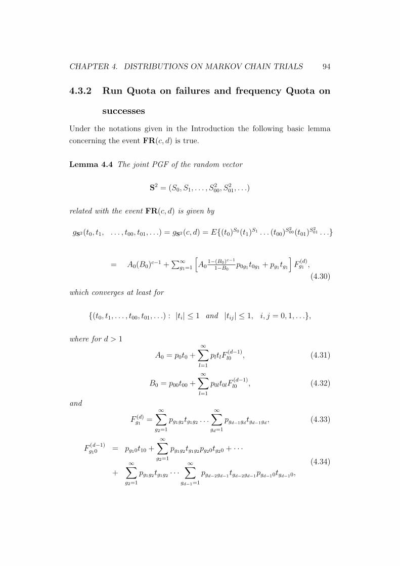
CHAPTER 4. DISTRIBUTIONS ON MARKOV CHAIN TRIALS 94
4.3.2 Run Quota on failures and frequency Quota on
successes
Under the notations given in the Introduction the following basic lemma
concerning the event FR(c, d) is true.
Lemma 4.4 The joint PGF of the random vector
S2 = (S0, S1, . . . , S200, S
201, . . .)
related with the event FR(c, d) is given by
gS2(t0, t1, . . . , t00, t01, . . .) = gS2(c, d) = E(t0)S0(t1)S1 . . . (t00)S200(t01)S
201 . . .
= A0(B0)c−1 +∑∞
g1=1
[A0
1−(B0)c−1
1−B0p0g1t0g1 + pg1tg1
]F
(d)g1 ,
(4.30)
which converges at least for
(t0, t1, . . . , t00, t01, . . .) : |ti| ≤ 1 and |tij| ≤ 1, i, j = 0, 1, . . .,
where for d > 1
A0 = p0t0 +∞∑l=1
pltlF(d−1)l0 , (4.31)
B0 = p00t00 +∞∑l=1
p0lt0lF(d−1)l0 , (4.32)
and
F (d)g1
=∞∑g2=1
pg1g2tg1g2 . . .
∞∑gd=1
pgd−1gdtgd−1gd , (4.33)
F(d−1)g10 = pg10t10 +
∞∑g2=1
pg1g2tg1g2pg20tg20 + · · ·
+∞∑g2=1
pg1g2tg1g2 · · ·∞∑
gd−1=1
pgd−2gd−1tgd−2gd−1
pgd−10tgd−10,
(4.34)

CHAPTER 4. DISTRIBUTIONS ON MARKOV CHAIN TRIALS 95
for g1 = 1, 2, . . . .
If d = 1, F(d)g1 = 1 and F
(d−1)g10 = 0.
Proof. The joint PGF (4.30) can be obtained by symmetry with the joint
PGF (4.21).
The expression (4.33) for F(d)g1 represents the contribution to the joint PGF
when d−1 consecutive failure states follow the failure state g1, g1 = 1, 2, . . ..
In this case all possible outcomes terminate with d consecutive failures. By
analogy, relation (4.34) for F(d)g10 is the contribution to the joint PGF when
the Markov chain moves from some failure state g1 = 1, 2, . . . to a successive
one, with preceded subsequences containing no more than d− 2 consecutive
failures.
Then A0 given by (4.31) is the contribution to the joint PGF gS2(c, d)
until the Markov chain moves to the first successive state and B0 given by
(4.32) is the corresponding contribution when the Markov chain moves from
the successive state to the next successive state in the possible sequences of
outcomes.
The relation (4.30) is a PGF, since the following relations
F(d−1)g10 (1) + F (d)
g1(1) = 1 (4.35)
and
1−B0(1) =∞∑g1=1
p0g1F(d)g1
(1)
are true for g1 = 1, 2, . . . , where 1 means the corresponding unit vector. This
completes the proof.
2
Remark 4.15 The total number of successes X in the event FR(c, d) may
be represented by the following equation
X = S0 +∞∑g1=0
S2g10.

CHAPTER 4. DISTRIBUTIONS ON MARKOV CHAIN TRIALS 96
Now, evaluating gS2(c, d) at the appropriate values we obtain the following
exact distribution
P (X = 0) = a1(d);
P (X = 1) = A0(1)a0(d);
P (X = x) = A0(1)(B0(1))x−1a0(d), for x = 2, 3, . . . , c− 1;
P (X = c) = A0(1)(B0(1))c−1,
where 1 means the corresponding unit vector,
a1(d) =∞∑g1=1
pg1F(d)g1
(1) and a0(d) =∞∑g1=1
p0g1F(d)g1
(1).
Remark 4.16 Let us consider a Markov chain with a matrix of transition
probabilities from Example 4.3. We will give the corresponding formulas when
d takes values 2, 3 and 4.
If d = 2, from (4.31) and (4.32) we have
A0(1) = p0 + p1p10 and B0(1) = p00 + p01p10.
The exact distribution of the number of successes from Remark 4.15 can be
obtained with
a1(2) = p1p12 and a0(2) = p01p12.
If d = 3, the corresponding relations are given by
A0(1) = p0 + p1(p10 + p12p20);
B0(1) = p00 + p01(p10 + p12p20);
a1(3) = p1p12p222;
a0(3) = p01p12p222.

CHAPTER 4. DISTRIBUTIONS ON MARKOV CHAIN TRIALS 97
Finally, if d = 4 we have
A0(1) = p0 + p1(p10 + p12p20 + p12p22p20);
B0(1) = p00 + p01(p10 + p12p20 + p12p22p20);
a1(4) = p1p12p22;
a0(4) = p01p12p22.
Remark 4.17 Let us consider the following particular cases of (4.30):
– first, let d −→ ∞. For g1 = 1, 2, . . . , (4.34) gives F(∞)g10 (1) = 1, since
our assumption for persistent states of the Markov chain. Then from (4.35)
we have
limd−→∞
F (d)g1
(1) = 0
and therefore from (4.33) it is fulfilled
limd−→∞
F (d)g1
= 0,
for g1 = 1, 2, . . . . This limiting case yields the following joint PGF
g2(c,∞) = A0(∞)(B0(∞))c−1, (4.36)
where A0(∞) and B0(∞) are derived from (4.31) and (4.32) respectively, by
putting d −→∞.
– second, letting c −→ ∞ in (4.30) yields the following joint PGF until
d consecutive failures are observed in a multi - state Markov chain
g2(∞, d) =∞∑g1=1
[A0
1−B0
p0g1t0g1 + pg1tg1
]F (d)g1. (4.37)

CHAPTER 4. DISTRIBUTIONS ON MARKOV CHAIN TRIALS 98
Remark 4.18 By symmetry, the joint PGF g2L(c, d) related with the later
occurring event
FRL(c, d) =
the trials are performed sequentially
until both c successes in total and
d consecutive failures are observed
has the representation
g2L(c, d) = g2(c,∞) + g2(∞, d)− gS2(c, d),
where gS2(c, d), g2(c,∞) and g2(∞, d) are the joint PGF’s given by (4.30),
(4.36) and (4.37), correspondingly.
4.3.3 Comments
In this chapter the geometric distribution of order k related to multi - state
Markov chain is defined. The main result is Lemma 4.1. As a Corollary of
the lemma, the PGFs of the number of successes, the number of failures and
the number of trials (geometric distribution of order k) are given in Theorem
4.1, Theorem 4.2 and Theorem 4.3. The joint distribution of the number of
successes and the number of failures is given in the Theorem 4.4. The result
is published in [47] and [48]. The application in quality control is mentioned
in [87].
The sooner and later waiting time problems discussed by Balasubrama-
nian et al. [12] and Aki and Hirano [3] have been generalized to the multi -
state Markov chain, published in [49]. The main result is in Lemma 4.2. In
this case the PGFs of the number of successes and the number of failures are
given.
The obtained results can be applied for evaluating the system reliability
(start - up demonstration tests), molecular biology (modeling the structure
of DNA), for description of some random walk models, etc.

CHAPTER 4. DISTRIBUTIONS ON MARKOV CHAIN TRIALS 99
The waiting time problems related with run and frequency quotas have
been generalized to the multi - state Markov chain. The basic results stated
by Lemma 4.3 and Lemma 4.4 are published in [50].
Presented results can also be extended for non - overlapping way of count-
ing and for more complex sooner and latter waiting time problems considered
by Uchida and Aki [83] and Balakrishnan et al. [11].
Chapter 5
I - Stochastic processes
The family of IGPSDs, defined in Chapter 2 is a generalization of the the
family of GPSD, or the classical discrete distributions. Having in hand the
new family of distributions we ask the natural question: What will be the
corresponding generalization of the counting stochastic process.
5.1 The Polya - Aeppli process
The IPo(λ, ρ) distribution is a generalization of the classical Po(λ) distribu-
tion. As we mentioned in Remark 2.10 the IPo(λ, ρ) distribution coincides
with the Polya-Aeppli distribution. It was derived by Anscombe [6] in 1950,
who stated that it was given earlier by A. Aeppli in a thesis in 1923 and
then studied subsequently by G. Polya in 1930. For this reason, Anscombe
called this distribution a Polya - Aeppli distribution. In this section we will
define a generalization of the Poisson process and will call it a Polya - Aeppli
process.
Let us consider the sequence T1, T2, . . . of non - negative, mutually inde-
pendent random variables and the corresponding renewal process
Sn =n∑i=1
Ti, n = 1, 2 . . . , S0 = 0.
100
CHAPTER 5. I - STOCHASTIC PROCESSES 101
The process Sn can be interpreted as a sequence of renewal epochs. T1 is the
time until the first renewal epoch and Tii≥2 are the inter-arrival times.
Let N(t) = supn ≥ 0, Sn ≤ t, t ≥ 0 be the number of renewals
occurring up to time t. The distribution of N(t) is related to that of Sn, and
for any t ≥ 0 and n ≥ 0, the following probability relation holds:
P (N(t) = n) = P (Sn ≤ t)− P (Sn+1 ≤ t, n = 0, 1, 2, . . . . (5.1)
We will suppose that N(t) is described by the IPo(λt, ρ) distribution (or
Polya - Aeppli distribution), with mean function λ1−ρt, i.e.
P (N(t) = n) =
e−λt, n = 0
e−λtn∑i=1
(n− 1
i− 1
)[λ(1− ρ)t]i
i!ρn−i, n = 1, 2, . . . .
(5.2)
Let us denote by LSX(s) =∫∞
0e−sxdFX(x) the Laplace - Stieltjes trans-
form (LST) of any random variable X with distribution function FX(x). Let
Pn(t) = P (N(t) = n).
For the next considerations we need the following result.
Lemma 5.1 The LST of Pn(t) is given by
LSPn(t)(s) =
∫ ∞0
e−stdPn(t)
=
− λ
s+ λ, n = 0
(1− ρ)λ
s+ λ
s
s+ λ
[ρ+ (1− ρ)
λ
s+ λ
]n−1
, n = 1, 2, . . . .
Now we will show that the renewal process is characterized by the fact that
T1 is exponentially distributed and T2, T3, . . . are identically distributed.
Moreover, T2 is zero with probability ρ, and with probability 1− ρ exponen-
tially distributed with parameter λ. This means that the probability density
functions and the mean values are the following:
CHAPTER 5. I - STOCHASTIC PROCESSES 102
fT1(t) = λe−λt, t ≥ 0, ET1 =1
λ(5.3)
and
fT2(t) = ρδ0(t) + (1− ρ)λe−λt, t ≥ 0, ET2 =1− ρλ
, (5.4)
where
δ0(t) =
1, if t = 00, otherwise,
The process Sn is called a delayed renewal process with a delay T1.
Theorem 5.1 There exists exactly one renewal process such that the number
of renewals up to time t has the Polya - Aeppli distribution (5.2). In this
case the time until the first renewal epoch T1 is exponentially distributed with
parameter λ. The inter-arrival times T2, T3, . . . are equal to zero with prob-
ability ρ and with probability 1 − ρ exponentially distributed with parameter
λ.
Proof. To prove the theorem it suffices to show that the LST of the random
variable Sn is equal to
LSSn(s) =λ
s+ λ[ρ+ (1− ρ)
λ
s+ λ]n−1. (5.5)
We will prove it by induction using the relations (5.1). For n = 0 (5.1)
becomes
P (N(t) = 0) = 1− P (T1 ≤ t) = 1− FT1(t), (5.6)
where FT1(t) is the distribution function of T1. On the other hand, from (5.2)
it follows that
P (N(t) = 0) = e−λt. (5.7)
Combining (5.6) and (5.7) gives that FT1(t) = 1 − e−λt, i.e. the r.v. T1 is
exponentially distributed with parameter λ and LST λs+λ
.
Now from (5.1), for n = 1, we get
P (N(t) = 1) = P (S1 ≤ t)− P (S2 ≤ t).

CHAPTER 5. I - STOCHASTIC PROCESSES 103
Taking the LST leads to
(1− ρ)λ
s+ λ
s
s+ λ= LSS1(s)− LSS2(s).
After some algebra we arrive at
LST1+T2(s) =λ
s+ λ[ρ+ (1− ρ)
λ
s+ λ],
which means that T2 is independent of T1. Moreover, T2 is exponentially
distributed random variable with parameter λ and mass at zero equal to ρ.
The probability density function of T2 is given by (5.4).
Let suppose now that for any n ≥ 2, the LST of Sn is given by (5.5).
Taking the LST in (5.1) we get
LSSn+1(s) =
∫ ∞0
e−stdP (Sn+1 ≤ t)
=
∫ ∞0
e−stdP (Sn ≤ t)−∫ ∞
0
e−stdPn(t).
Applying Lemma 5.1 one can show that the LST of the renewal process
Sn+1 is equal to
LSSn+1(s) =λ
s+ λ
[ρ+ (1− ρ)
λ
s+ λ
]n.
This proves the theorem.
2
Remark 5.1 In the case of ρ = 0, the LST (5.5) becomes the LST of
Gamma(n, λ) (or Erlang (n)) distributed random variable. This case co-
incides with the usual homogeneous Poisson process.
Remark 5.2 Let us note that the probability distribution function of T2 is
given by
FT2(t) = 1− (1− ρ)e−λt, t ≥ 0.
That family of distributions has a jump at zero. That is, P (T2 = 0) = ρ.

CHAPTER 5. I - STOCHASTIC PROCESSES 104
Remark 5.3 It is easy to see that the exponential distribution function of
the delay, FT1(t), and the distribution function FT2(t), satisfy the following
relation:
FT1(t) =1
ET2
∫ t
0
[1− FT2(u)]du. (5.8)
In this case the delayed renewal counting process is the only stationary re-
newal process, see [21]. From the renewal theory, it is known, that under the
condition (5.8), the delayed renewal counting process has stationary incre-
ments, see for instance Rolski et al. [77], Theorem 6.1.8.
We proved the theorem using the LST and basic relation (5.1). The
converse theorem is also true.
Theorem 5.2 Let suppose that the inter-arrival times Tii≥2 of the station-
ary renewal process are equal to zero with probability ρ and with probability
1−ρ exponentially distributed with parameter λ. Then the number of renewals
up to time t, has the Polya - Aeppli distribution.
Now we can define the inflated - parameter Poisson process, or the Polya
- Aeppli process.
Definition 5.1 A counting process N(t), t ≥ 0 is said to be a Polya -
Aeppli process if
(a) it starts at zero, N(0) = 0;
(b) it has independent, stationary increments;
(c) for each t > 0, N(t) is Polya - Aeppli distributed.
The Polya - Aeppli process is a time homogeneous process, such that i
claims can arrive simultaneously with probability ρi−1, for i = 1, 2, . . .. In
the case of ρ = 0 it becomes a homogeneous Poisson process. So, we have a
homogeneous process with an additional parameter ρ.

CHAPTER 5. I - STOCHASTIC PROCESSES 105
Remark 5.4 In the definition of the Polya - Aeppli process, the parameter
ρ is interpreted as a probability and we assume that ρ ∈ [0, 1). At the same
time we started with the interpretation of ρ as a correlation coefficient in a
Markov chain. Let us suppose that the correlation coefficient is r ∈ (−1, 1).
In this case the parameter ρ is equal to ρ = |r| and the given definitions and
properties are fulfilled.
5.1.1 Moments
The mean value and the variance of Polya - Aeppli process are given by
EN(t) =λ
1− ρt and V ar(N(t)) =
λ(1 + ρ)
1− ρt.
The index of dispersion is
V ar(N(t))
EN(t)=
1 + ρ
1− ρ> 1,
i.e. the Polya - Aeppli process is overdispersed relative the Poisson process.
5.2 I - Polya process
In this section we will obtain the Inflated - parameter negative binomial
process, called also I - Polya process by mixing the Polya - Aeppli process.
Suppose that the number of items in the time interval [0, t] has a conditional
Polya - Aeppli distribution, i.e.
P (Nt = m | λ) =
e−λt, m = 0,
e−λt∑m
i=1
(m−1i−1
)[λ(1−ρ)t]i
i!ρm−i, m = 1, 2, . . . ,
(5.9)
where λ > 0 and ρ ∈ [0, 1). The mean number of arrivals is E(Nt | λ) = λ1−ρt.
Suppose that λ is the outcome of a random variable Λ. Following the
well known terminology [45] the resulting process is a mixed Polya - Aeppli
process. The probability distribution Λ is called mixing distribution. The

CHAPTER 5. I - STOCHASTIC PROCESSES 106
PMF (5.9) is interpreted as the conditional distribution of Nt, given the
outcome Λ = λ.
Let the distribution of the mixing random variable Λ be gamma one with
parameters β and r. Its probability density function is given by
βr
Γ(r)λr−1e−βλ, β > 0, λ > 0,
where Γ(r) is the Gamma function, r is called the shape parameter and β
the scale parameter.
In this case Nt has the following probability mass function:
P (Nt = m) =
(
ββ+t
)r, m = 0(
ββ+t
)r∑mi=1
(m−1i−1
)(r+i−1i
)[(1− ρ) t
β+t]iρm−i, m = 1, 2, . . . .
(5.10)
This is just the Inflated - parameter negative binomial distribution with
parameters ββ+t
, ρ and r, INB( ββ+t
, ρ, r). In the case of ρ = 0 (5.10) coincides
with the usual negative binomial distribution with parameters ββ+t
and r.
If the number of events up to time t is negative binomial distributed, the
counting process is known as Polya process, see [37], p. 4. This motivated
the following definition.
Definition 5.2 The counting process, N(t), t ≥ 0 is said to be an Inflated
- parameter Polya process or I - Polya process, if it starts at zero, N(0) = 0
and for each t > 0, the distribution of N(t) is given by (5.10).
5.2.1 Properties of the I - Polya process
Denote Sn = T1 + T2 + . . .+ Tn, n = 1, 2, . . . , the waiting time until the nth
event. The basic properties of the I - Polya process are given by the next
theorem.
Theorem 5.3 Let N(t) has the INB( ββ+t
, ρ, r)distribution (5.10). Then
CHAPTER 5. I - STOCHASTIC PROCESSES 107
(i) The time until the first epoch T1 is Pareto distributed. The inter-
arrival times T2, T3, . . . are zero with probability ρ and with probability 1− ρ
Pareto distributed.
(ii) The waiting time until the nth event has the following probability
density function
fSn(t) =n−1∑i=0
(n− 1
i
)(1−ρ)iρn−1−i r
β
(r + i
i
)(β
β + t
)r+1(t
β + t
)i. (5.11)
Proof. (i) According to the definition of the Polya - Aeppli process the
conditional distribution of T1 is exp(λ). The unconditional distribution is
given by the probability distribution function
FT1(t) =
∫ ∞0
(1− e−λt) βr
Γ(r)λr−1e−βλdλ = 1−
(β
β + t
)r, t ≥ 0 (5.12)
and the probability density function
fT1(t) =r
β
(β
β + t
)r+1
, t ≥ 0.
We write T1 ∼ P (β, r) for Pareto distribution with parameters β and r.
Similarly for the distribution of T2 we obtain
FT2(t) = 1− (1− ρ)
(β
β + t
)r, t ≥ 0 (5.13)
and
fT2(t) = ρδ(0) + (1− ρ)r
β
(β
β + t
)r+1
, t ≥ 0
where δ(x) is the delta function. T2 is Pareto distributed with mass at zero
equal to ρ.
(ii) We will prove (5.11) by induction, using the following relation
P (Sn+1 ≤ t) = P (Sn ≤ t)− P (N(t) = n), n = 0, 1, 2, . . . . (5.14)
For n = 1 (5.14) becomes
P (S2 ≤ t) = P (S1 ≤ t)− P (N(t) = 1). (5.15)

CHAPTER 5. I - STOCHASTIC PROCESSES 108
According to (5.10)
P (N(t) = 1) = r(1− ρ)
(β
β + t
)rt
β + t.
The random variable S1 coincides with the random variable T1. Differenti-
ating (5.14) and rearranging the terms leads to
fS2(t) = ρr
β
(β
β + t
)r+1
+ (1− ρ)r(r + 1)
β
(β
β + t
)r (t
β + t
).
Suppose now that (5.11) is true. Differentiating (5.14) and applying (5.10)
and (5.11) we find that
fSn+1(t) =n∑i=0
(n
i
)(1− ρ)iρn−i
r
β
(r + i
i
)(β
β + t
)r+1(t
β + t
)i.
2
5.2.2 Moments
The mean value and the variance of I - Polya process are given by
EN(t) =r
(1− ρ)
t
β
and
V ar(N(t)) =r
(1− ρ)
t
β
[(1 + ρ)β + t
(1− ρ)β
]= EN(t)
[1 + ρ
1− ρ+
t
(1− ρ)β
]The index of dispersion
V ar(N(t))
EN(t)>
1 + ρ
1− ρ.
This means that the I - Polya process is overdispersed relative the Polya -
Aeppli process.

CHAPTER 5. I - STOCHASTIC PROCESSES 109
5.3 I - Binomial process
Suppose that N(t) =∑N1(t)
i=1 Yi, where Y1, Y2, . . . are independent identically
distributed random variables, independent of N1(t). Let for α > 0, t < α and
n ≥ 1, N1(t) has a binomial distribution with parameters n and tα
(N1(t) ∼Bi(n, t
α)). Let Y denotes the compounding random variable. Here we suppose
that for ρ ∈ [0, 1), Y is geometrically distributed with success probability
1− ρ (Y ∼ Ge1(1− ρ)), and has a probability mass function
P (Y = i) = (1− ρ)ρi−1, i = 1, 2, . . . .
The compound binomial process N(t) has Inflated - parameter binomial
distribution and is called Inflated - parameter binomial process or I-Binomial
process. The distribution is given by
P (Nt = m) =
(
1− t
α
)n, m = 0
m∧n∑i=1
(n
i
)(m− 1
i− 1
)[(1− ρ)
t
α
]i(1− t
α
)n−iρm−i, m = 1, 2, . . . .
(5.16)
The I-Binomial process is not a simple process and the probability that
two or more claims can arrive simultaneously is greater than zero.
This leads to the following definition
Definition 5.3 The counting process N(t), t ≥ 0 is said to be I - Binomial
process, if it starts at zero, N(0) = 0 and for each t ∈ (0, α), the distribution
of N(t) is given by (5.16).
5.3.1 Properties of the I-Binomial process
Denote Sm = T1 + T2 + . . . + Tm, m = 1, 2, . . . , the waiting time until the
mth event. One of the basic properties of the I-Binomial process is given in
the next theorem.

CHAPTER 5. I - STOCHASTIC PROCESSES 110
Theorem 5.4 Let N(t) has the IBi( tα, ρ, n)distribution (5.16). Then the
waiting time until the mth event for m ≥ 1 and t < α has the following
probability density function
fSm(t) =n
α
(m−1)∧(n−1)∑i=0
(n− 1
i
)(m− 1
i
)[(1− ρ)
t
α
]i(1− t
α
)n−i−1
ρm−i−1.
(5.17)
Proof. We will prove (5.17) by induction, using the following relation
P (Sm+1 ≤ t) = P (Sm ≤ t)− P (N(t) = m), m = 0, 1, 2, . . . . (5.18)
For m = 1 (5.18) becomes
P (S2 ≤ t) = P (S1 ≤ t)− P (N(t) = 1). (5.19)
According (5.16)
P (N(t) = 1) = n(1− ρ)t
α
(1− t
α
)n−1
. (5.20)
The random variable S1 coincides with the random variable T1. From
(5.18) for m = 0 we get
P (S1 ≤ t) = 1− P (N(t) = 0) = 1−(
1− t
α
)n. (5.21)
Substituting (5.20) and (5.21) in (5.19) we obtain
P (S2 ≤ t) = 1−[1− (1− (1− ρ)n)
t
α
](1− t
α
)n−1
. (5.22)
Differentiating (5.22) we get the pdf of S2 + T1 + T2
fS2(t) = ρn
α
(1− t
α
)n−1
+ (1− ρ)n(n− 1)
α
t
α
(1− t
α
)n−2
, t < α.
Let suppose now that (5.17) is true. Differentiating the relation
FSm+1(t) = FSm(t)− P (N(t) = m)

CHAPTER 5. I - STOCHASTIC PROCESSES 111
and applying (5.16) and (5.17) we find that
fSm+1(t) =n
α
m∧(n−1)∑i=0
(m
i
)(n− 1
i
)[(1− ρ)
t
α
]i(1− t
α
)n−i−1
ρm−i.
This completes the proof.
2
Corollary 5.1 The time until the first claim T1 has the following density
function
fT1(t) =n
α
(1− t
α
)n−1
, t < α. (5.23)
Proof. Differentiating (5.21), leads to (5.23).
2
5.3.2 Moments
The mean value and the variance of I - Binomial process are given by
EN(t) =nt
(1− ρ)α
and
V ar(N(t)) =n
(1− ρ)2
[1− t
α+ ρ
]t
α= EN(t)
[1 + ρ
1− ρ− t
(1− ρ)α
].
If the index of dispersion
V ar(N(t))
EN(t)=
1 + ρ
1− ρ− t
(1− ρ)α> 1,
then the variance is larger than the mean and ρ > t2α. In this case the I-
Binomial process is overdispersed. If ρ < t2α, the process is underdispersed.
CHAPTER 5. I - STOCHASTIC PROCESSES 112
5.4 Inflated - parameter modification of the
pure birth process
In this section we give a new interpretation of the defined processes.
To begin, let N(t) represents the state of the system at time t ≥ 0. It
is assumed that the process has state space N , the non-negative integers.
Let λi(t) > 0, i = 1, 2, . . . be any given functions of t, called intensity of
(transition) frequencies, and ρ ∈ (0, 1).
We assume the following postulates:
P (N(t+h) = n | N(t) = m) =
1− (1− ρ)
∑∞i=1 λi(t)ρ
i−1h+ o(h), n = m,(1− ρ)ρi−1λi(t)h+ o(h), n = m+ i,
i = 1, 2, . . . ,
for every m = 0, 1, . . ., where o(h)→ 0 as h→ 0.
Let Pm(t) = P (N(t) = m), m = 0, 1, 2, . . .. Then the above postulates
yield the following Kolmogorov forward equations:
P ′0(t) = −(1− ρ)∑∞
i=1 λi(t)ρi−1P0(t),
P ′m(t) = −(1− ρ)∑∞
i=1 λi(t)ρi−1Pm(t) + (1− ρ)
∑mi=1 λi(t)ρ
i−1Pm−i(t),(5.24)
for m = 1, 2, . . . , with the conditions
P0(0) = 1 and Pm(0) = 0, m = 1, 2, . . . . (5.25)
We call the process defined by (5.24) and (5.25) an Inflated - parameter
modification of the pure birth process (or I - modification).
In the next we consider particular cases, useful for risk theory and queue-
ing theory.
The Polya-Aeppli process. Let us suppose that the functions λi(t) = λ
are constants for every i = 1, 2 . . .. In this case the Kolmogorov equations
(5.24) are given by
P ′0(t) = −λP0(t),
P ′m(t) = −λPm(t) + (1− ρ)λm∑i=1
ρi−1Pm−i(t), m = 1, 2, . . . .

CHAPTER 5. I - STOCHASTIC PROCESSES 113
Integrating the above system of differential equations with the conditions
(5.25) we obtain the distribution (5.2), i. e.
P (N(t) = m) =
e−λt, m = 0
e−λt∑m
i=1
(m−1i−1
) [(1−ρ)λt]i
i!ρm−i, m = 1, 2, . . . .
The I-Polya process. Let the intensity functions λi(t), i = 1, 2, . . .
depend on t in the following way
λi(t)ρi−1 =
r
β
(β
β + t
)2(1− (1− ρ)
β
β + t
)i−1
, t ≥ 0, (5.26)
where β > 0 is a parameter, and λi(t)ρi−1 → 0, as t→∞.
The Kolmogorov equations (5.24) become
P ′0(t) = − r
β + tP0(t),
P ′m(t) = − r
β + tPm(t)
+ (1− ρ)r
β
(β
β + t
)2 m∑i=1
(1− (1− ρ)
β
β + t
)i−1
Pm−i(t),m = 1, 2, . . . .
By integrating we obtain the explicit solutions
P (N(t) = m) =
(
ββ+t
)r, m = 0(
ββ+t
)r∑mi=1
(m−1i−1
)(r+i−1i
)[(1− ρ) t
β+t]iρm−i, m = 1, 2, . . . ,
which can be easily verified by insertion into the system. This is the INB( ββ+t
, ρ, r)
distribution (5.10), where π = ββ+t
.
The Inflated-parameter binomial process. Let the functions λi(t), i =
1, 2, . . . depend on t in the following way
λi(t)ρi−1 =
n
α
(α
α− t
)2(1− (1− ρ)
α
α− t
)i−1
, (5.27)
where α > 1 is a parameter and t < α. In this case λi(t)ρi−1 →∞ as t→ α.
The Kolmogorov differential equations in this case are the following
P ′0(t) = − n
α− tP0(t),
P ′m(t) = − n
α− tPm(t)
+ (1− ρ)n
α
(α
α− t
)2 m∑i=1
(1− (1− ρ)
α
α− t
)i−1
Pm−i(t),m = 1, 2, . . . .

CHAPTER 5. I - STOCHASTIC PROCESSES 114
Integrating and applying the conditions (5.25) we obtain the IBi( tα, ρ, n)
distribution (5.16) for π = tα.
5.5 Generalized Delaporte distribution.
In this section we introduce a generalization of one very popular counting
distribution. The Delaporte distribution, (see [78] and [38]), is a mixed
Poisson distribution with shifted Gamma mixing distribution. Here we also
suppose that the mixing distribution is a shifted Gamma distribution with
probability density function given by
βr
Γ(r)(λ− α)r−1e−β(λ−α), β > 0, λ ≥ α.
The parameter α can be interpreted as a basic risk, [38]. We suppose that
Nt is a Polya - Aeppli process. The unconditional probability mass function
in this case is the following:
P (Nt = m) =
∫ ∞α
P (Nt = m | λ)βr
Γ(r)(λ− α)r−1e−β(λ−α)dλ. (5.28)
Calculating the integral in (5.28) gives the following probability mass
function
P (Nt = m)
=
e−αt(
β
β + t
)r, m = 0
e−αt(
β
β + t
)r [r(1− ρ)
t
β + t+ α(1− ρ)t
], m = 1
e−αt(
β
β + t
)r [ m∑i=1
(m− 1
i− 1
)(r + i− 1
i
)((1− ρ)
t
β + t
)iρm−i
+m∑i=1
(m− 1
i− 1
)[α(1− ρ)t]i
i!ρm−i +
m−1∑i=1
i∑j=1
(i− 1
j − 1
)[α(1− ρ)t]j
j!ρi−j
×m−i∑k=1
(m− i− 1
k − 1
)(r + k − 1
k
)((1− ρ)
t
β + t
)kρm−i−k
], m = 2, 3, . . . .

CHAPTER 5. I - STOCHASTIC PROCESSES 115
The random variable Nt in this case is a sum of an IPo(αt, ρ) variable
and independent INB( ββ+t
, ρ, r) variable.
In the case ρ = 0 the distribution coincides with the Delaporte distribu-
tion, see [38]. So we say that the above random variable Nt has a generalized
Delaporte distribution (I - Delaporte distribution).
Taking ρ = 0 in the above processes we obtain the homogeneous Pois-
son process, Polya process and binomial process, respectively. The relation-
ships between I - processes are similar as between their classical analogues.
In all the cases the parametrization is chosen to ensure constant intensity
( ddtN(t) = const). We say that the Polya - Aeppli process is a stationary re-
newal process. The I - Polya and I - binomial can be interpreted as renewal
processes with dependency.
5.6 Stochastic processes of order k
5.6.1 Polya - Aeppli process of order k
Let N(t) represents the state of the system at time t ≥ 0. It is assumed that
the process has state space N , the non-negative integers. Let λ > 0 be any
real number and ρ ∈ [0, 1).
Suppose that N(t) has a PAk(λt, ρ) distribution. The PGF of N(t) is
given by
h(u, t) = eλt[PX(u)−1], (5.29)
where PX(u) is the PDF of the truncated geometric distribution
PX(t) =(1− ρ)t
1− ρk1− ρktk
1− ρt. (5.30)
Definition 5.4 A compound Poisson process with truncated geometric com-
pounding distribution is called Polya - Aeppli process of order k.

CHAPTER 5. I - STOCHASTIC PROCESSES 116
The second definition of the process is as a pure birth process. The
properties of the defined process are specified by the following postulates:
P (N(t+ h) = n | N(t) = m) =
1− λh+ o(h), n = m,1−ρ1−ρk ρ
i−1λh+ o(h), n = m+ i,
i = 1, 2, . . . , k
for every m = 0, 1, . . . , where o(h) → 0 as h → 0. Note that the postulates
imply that for i = k+ 1, k+ 2, . . . , P (N(t+ h) = m+ i | N(t) = m) = o(h).
According to the postulates, the probability that 2, 3, . . . k claims to the
insurance company arrive simultaneously is positive.
Let Pm(t) = P (N(t) = m), m = 0, 1, 2, . . . . Then the above postulates
yield the following Kolmogorov forward equations:
P ′0(t) = −λP0(t),
P ′m(t) = −λPm(t) + 1−ρ1−ρkλ
∑m∧kj=1 ρ
j−1Pm−j(t), m = 1, 2, . . . ,(5.31)
with the conditions
P0(0) = 1 and Pm(0) = 0, m = 1, 2, . . . . (5.32)
Let
h(u, t) =∞∑m=0
umPm(t)
be the PGF of the process N(t). Multiplying the mth equation of (5.31)
by um and summing for all m = 0, 1, 2, . . . we get the following differential
equation∂h(u, t)
∂t= −λ[1− PX(u)]h(u, t). (5.33)
The solution of (5.33) with the initial condition
P0(0) = 1
is
h(u, t) = e−λt[1−PX(u)],
which is the PGF of the PAk(λt, ρ) distribution, given by (5.29) and (5.30).

CHAPTER 5. I - STOCHASTIC PROCESSES 117
Definition 5.5 The birth process defined by (5.31) and (5.32) is called a
Polya - Aeppli process of order k.
Remark 5.5 In the case of k → ∞, the Polya - Aeppli process of order
k, coincides with the Polya - Aeppli process. If ρ = 0, it is a homogeneous
Poisson process.
5.7 Comments
The Polya - Aeppli process with characterization and the properties are given
in [61]. The I - stochastic processes, defined in this chapter are published
in [58]. The I - Polya process with applications in Risk theory is given also
in [65]. In [28], Dragieva described the Polya - Aeppli process as an input
process in a queueing system. The Polya - Aeppli process of order k is defined
in [63].

Chapter 6
Risk Models
Consider the standard model of an insurance company, called risk process
X(t), t ≥ 0, defined on the complete probability space (Ω,F , P ), and given
by the equation (1.1)), i.e.
X(t) = ct−N(t)∑i=1
Zi, (0∑1
= 0).
The risk process X(t) represents the profit of the risky business in (0, t].
The random variables Zi∞i=1 are mutually independent, identically dis-
tributed with common distribution function F , F (0) = 0, and mean value
µ. In this chapter we consider several examples of the counting process
N(t), t ≥ 0. A common used measure of the risk related to an insurance
company is the ruin probability. Denote by
τ(u) = inft > 0, u+X(t) ≤ 0
the time to ruin of a company having initial capital u. We let τ =∞, if for
all t > 0 u+X(t) > 0.
The ruin probability Ψ(u) in the infinite horizon case for the insurance
company with initial capital u is defined by
Definition 6.1
Ψ(u) = P (τ(u) <∞).
118
CHAPTER 6. RISK MODELS 119
Sometimes it is more convenient to use the probability of non ruin Φ(u) =
1−Ψ(u).
From the definition it follows that Ψ(u) = 1 for u < 0. We suppose that
u ≥ 0.
The relative safety loading coefficient θ of the insurance company is de-
fined by
θ =EX(t)
E(∑N(t)
i=1 Zi). (6.1)
The risk process X(t) has a positive safety loading, if θ > 0. In this case X(t)
has a trend to +∞ and we say that there is a net profit condition, (NPC).
6.1 The Polya - Aeppli risk model
Suppose that the counting process N(t) in the risk process is the Polya -
Aeppli process independent of the claim sizes Zi∞i=1. We will call this
process a Polya - Aeppli risk process.
The relative safety loading θ is defined by
θ =c(1− ρ)− λµ
λµ=c(1− ρ)
λµ− 1, (6.2)
and in the case of positive safety loading θ > 0, c > λµ1−ρ .
The occurrence of the claims in the risk process (1.1) is described by a
delayed renewal counting process. We will study the ruin probability in two
cases following the renewal arguments, described by Feller [32] and Grandell
[37]. The main in the two cases is to derive the integral equations of ruin
probability.
6.1.1 The ordinary case
We suppose that the first claim has occurred and the subsequent claims occur
as an ordinary renewal process. The inter - occurrence times Tk, k = 1, 2, . . .
CHAPTER 6. RISK MODELS 120
are exponentially distributed with mass at zero equal to ρ and probability
density function, given by
fT2(t) = ρδ0(t) + (1− ρ)λe−λt, t ≥ 0, ET2 =1− ρλ
.
The claim sizes Z1, Z2, . . . are independent and identically distributed random
variables with common distribution function F (x) with F (0) = 0 and mean
value µ. Let
FI(x) =1
µ
∫ x
0
[1− F (z)]dz
be the integrated tail distribution. Let us define the function
H(z) = ρF (z) +λµ
cFI(z) (6.3)
and note that
H(∞) = ρF (∞) +λ
c
∫ ∞0
[1− F (z)]dz = ρ+λµ
c< 1.
If we denote by Φ0(u) and Ψ0(u) the non-ruin and ruin probabilities,
respectively, in the ordinary case, then the following result holds.
Proposition 6.1 The non-ruin function Φ0(u) satisfies the integral equation
Φ0(u) = Φ0(0) +
∫ u
0
Φ0(u− z)dH(z), u ≥ 0, (6.4)
where H(z) is defined by (6.3).
Proof. Suppose that the first claim occurs at epoch s. For no ruin to occur
according to the renewal argument we get
Φ0(t) =
∫ ∞0−
[ρδ0 + (1− ρ)λe−λs]
∫ t+cs
0
Φ0(t+ cs− z)dF (z)ds
= ρ
∫ t
0−Φ0(t−z)dF (z)+(1−ρ)
∫ ∞0−
λe−λs∫ t+cs
0
Φ0(t+cs−z)dF (z)ds, t ≥ 0.
Change of variables and differentiation leads to
Φ0′(t) = ρΦ0(0)F ′(t)+ρ
∫ t
0−Φ0′(t−z)dF (z)+
λ
c[Φ0(t)−λ
c
∫ t
0
Φ0(t−z)dF (z)],
(6.5)

CHAPTER 6. RISK MODELS 121
where Φ0′(t) is the derivative of Φ0(t). Integrating (6.5) in t over [0, u] and
performing integration by parts one gets
Φ0(u) = Φ0(0) + ρ
∫ u
0−Φ0(u− z)dF (z) +
λ
c
∫ u
0
Φ0(u− z)[1− F (z)]dz,
which is just equation (6.4).
2
Corollary 6.1 The ruin probability Ψ0(u) satisfies the following integral
equation:
Ψ0(u) = H(∞)−H(u) +
∫ u
0
Ψ0(u− z)dH(z), u ≥ 0. (6.6)
Proof. Equation (6.6) follows directly from (6.4).
2
Since H(∞) < 1, equations (6.4) and (6.6) are defective renewal equa-
tions.
Recalling that H(∞) = ρ + λµc
and Φ0(∞) = 1, in the case of positive
safety loading we conclude that
Φ0(0) = 1−H(∞) = (1− ρ)
[1− λµ
c(1− ρ)
],
and
Ψ0(0) = 1− Φ0(0) = H(∞).
Define LΦ0(s) =∫∞
0e−sxΦ0(x)dx to be the Laplace transform (LT) of
Φ0(u). Taking the LT of (6.4) we get
LΦ0(s) =Φ0(0)
s[1− LSH(s)], (6.7)
where LSH(s) is the LST of H(u). Using the standard properties of the
transforms and their inversions leads to
Φ0(u) = (1−H(∞))∞∑n=0
H∗n(u), u ≥ 0,

CHAPTER 6. RISK MODELS 122
where H∗n(u) means the n-th convolution of H(u) with itself. The same
result can be derived by using the fact that renewal equation (6.4) has an
unique solution, see for instance [?], Lemma 6.1.2.
Now let us define
H1(u) =H(u)
H(∞)=
H(u)
ρ+ λµc
,
which is a proper probability distribution. For the non-ruin probability we
have
Φ0(u) = [1−H(∞)]∞∑n=0
[H(∞)]nH∗n1 (u), u ≥ 0, (6.8)
and for the ruin probability
Ψ0(u) = [1−H(∞)]∞∑n=1
[H(∞)]nH∗n1 (u), u ≥ 0,
where H1(u) = 1−H1(u).
In the above formula we recognize a version of the Pollaczeck - Khinchin
formula (or Beekman convolution formula), see [77].
According to the definition of the relative safety loading (6.2), the follow-
ing relations hold:
1−H(∞) = (1− ρ)θ
1 + θand H(∞) =
1 + θρ
1 + θ.
So
Ψ0(u) = (1− ρ)θ
1 + θ
∞∑n=1
(1 + θρ
1 + θ
)nH∗n1 (u), u ≥ 0. (6.9)
In the case of ρ = 0, H1(u) = H(u) = G(u) and (6.9) coincides with the
ruin probability of the classical risk model.
Example 6.1 Let us consider the case of exponentially distributed claim
sizes, i.e. F (u) = 1 − e−uµ , u ≥ 0, µ > 0. In this case, the integrated
tail distribution FI(u) is exponential also and H(u) = (ρ+ λµc
)[1− e−uµ ]. So,
H1(u) = 1− e−uµ .

CHAPTER 6. RISK MODELS 123
Taking into account that the n-th convolution of H1(u) is an Erlang (n, 1µ
)
distribution with distribution function
H∗n1 (u) = 1− e−uµ
n−1∑j=0
(uµ
)jj!
,
relation (6.8) leads to
Φ0(u) = 1−H(∞) exp
−1−H(∞)
µu
.
The ruin probability in terms of the relative safety loading is given by
Ψ0(u) =1 + θρ
1 + θexp
−1− ρ
µ
θ
1 + θu
. (6.10)
If ρ = 0, the result coincides with the example of Grandell [37], p. 5-6
related to the ruin probability for the classical risk model. The example is to
be continued.
6.1.2 The stationary case
According to the arguments, described by Grandell [37], if Φ0(u) and Ψ0(u)
are non - ruin and ruin probability, respectively, in the ordinary case, then
in the stationary case we have the following result:
Proposition 6.2 The non-ruin probability Φ(u) and the ruin probability
Ψ(u) in the stationary case satisfy the integral representations
Φ(u) = Φ(0) +λ
c(1− ρ)
∫ u
0
Φ0(u− z)(1− F (z))dz (6.11)
and
Ψ(u) =λ
c(1− ρ)
[∫ ∞u
(1− F (z))dz +
∫ u
0
Ψ0(u− z)(1− F (z))dz
]. (6.12)

CHAPTER 6. RISK MODELS 124
Since Φ(∞) = Φ0(∞) = 1 when c > λµ1−ρ , we have
Φ(0) =1−H(∞)
1− ρ= 1− λµ
c(1− ρ).
Taking the Laplace transform of (6.11) and applying (6.7) we have
LΦ(s) =Φ(0)
s+
λµ
c(1− ρ)LSFI (s)
Φ0(0)
s[1− LSH(s)].
Again, the standard properties of the transforms lead to
LSΦ(s) =1−H(∞)
1− ρ+H(∞)− ρ
1− ρLSFI (s)[1−H∞)]
∞∑n=0
[LSH(s)]n.
So, the ruin probability in the stationary case is given by
Ψ(u) =H(∞)− ρ
1− ρ
[F I(u) + FI(u) ∗ [1−H(∞)]
∞∑n=1
[H(∞)]nH∗n1 (u)
],
(6.13)
where H1(u) = 1−H1(u) and F I(u) = 1− FI(u).
In terms of the relative safety loading the ruin probability is given by
Ψ(u) =1
1 + θF I(u) +
1
1 + θFI(u)
(1− ρ)θ
1 + θ
∞∑n=1
(1 + θρ
1 + θ
)nH∗n1 (u).
Example 6.2 Again, consider the case in which the claim amount distribu-
tion is exponential with mean value µ. Applying the argument of Example
6.1 to the ruin probability (6.13) yields
Ψ(u) =H(∞)− ρ
1− ρexp
−1−H(∞)
µu
,
and in terms of the relative safety loading,
Ψ(u) =1
1 + θexp
−1− ρ
µ
θ
1 + θu
. (6.14)
In the case of ρ = 0, (6.14) coincides with that of example 6 of Grandell [37],
p. 69.

CHAPTER 6. RISK MODELS 125
6.1.3 The Cramer - Lundberg approximation
6.1.3.1 The ordinary case
Let us return to the defective integral equation (6.6) for the ruin probability
in the ordinary case. Assume that there exists a constant R > 0 such that∫ ∞0
eRzdH(z) = 1, (6.15)
where H(z) is given by (6.3), and denote h(R) =∫∞
0eRzdF (z) − 1. The
equation (6.15) is known as a Cramer condition. For any functions f1(x)
and f2(x), we write f1(x) ∼ f2(x) for x→∞, if limx→∞f1(x)f2(x)
= 1.
Theorem 6.1 Let, for the Polya-Aeppli risk model, Cramer condition (6.15)
holds and h′(R) <∞. Then
Ψ0(u) ∼ µθA(µ, θ, R, ρ)
A2(µ, θ, R, ρ)h′(R)− µ(1 + θ)e−Ru, (6.16)
where A(µ, θ, R, ρ) = 1−[1−µ(1+θ)R]ρ1−ρ .
Proof. Multiplying (6.6) by eRu yields
eRuΨ0(u) = eRu(H(∞)−H(u)) +
∫ u
0
eR(u−z)Ψ0(u− z)eRzdH(z). (6.17)
It follows from the definition of R that the integral equation (6.17) is a
renewal equation.
The mean value of the probability distribution, given by
G(t) =
∫ t
0
eRzdH(z)
is ∫ ∞0
zeRzdH(z) =λ
cR
(1 +
c
λRρ)h′(R)− 1− ρ
R(1 + cλRρ)
.
Since ∫ ∞0
eRu(H(∞)−H(u))dz =1−H(∞)
R=
1− (ρ+ λµc
)
R,

CHAPTER 6. RISK MODELS 126
by the key renewal theorem, we have
Ψ0(u) ∼(1 + c
λRρ) (
(1− ρ) cλ− µ
)(1 + c
λRρ)2h′(R)− (1− ρ) c
λ
e−Ru.
Taking into account that cλ
= µ(1+θ)1−ρ we get the approximation (6.16) in
terms of the relative safety loading.
2
Definition 6.2 (6.16) is called a Cramer - Lundberg approximation.
The constant R, the non negative solution of the equation (6.15) is called a
Lundberg exponent or adjustment coefficient.
If ρ = 0, A(µ, θ, R, 0) = 1 and (6.16) coincides with the Cramer - Lund-
berg approximation for the classical risk model ([37], p. 7).
Example 6.3 If we take F (x) = 1 − exp(−xµ), then h(R) = µR
1−µR . The
constant R is a positive solution of the equation
(1 +c
λRρ)
µR
1− µR= (1− ρ)
c
λR, (6.18)
i.e.
R =1− ρµ
(1− λµ
c(1− ρ)
)=
1− ρµ
θ
1 + θ,
and A(µ, θ, R, ρ) = 1 + θρ.
So, the Cramer - Lundberg approximation is exact when the claims are
exponentially distributed and given by
Ψ0(u) ∼ 1 + θρ
1 + θe−Ru.

CHAPTER 6. RISK MODELS 127
6.1.3.2 The stationary case
Let us write integral representation (6.12) for the ruin probability in the
stationary case in the following equivalent form:
Ψ(u) =λµ
c(1− ρ)
[FI(u)−
∫ u
0
Ψ0(u− z)dFI(z)
].
Taking into account the Cramer - Lundberg approximation in the ordinary
case we have
Ψ(u) ∼(1− ρ) c
λ− µ(
1 + cλRρ)2h′(R)− (1− ρ) c
λ
e−Ru,
and in terms of the relative safety loading
Ψ(u) ∼ µθ
A2(µ, θ, R, ρ)h′(R)− µ(1 + θ)e−Ru. (6.19)
In the case of ρ = 0, asymptotic relation (6.19) coincides with the Cramer -
Lundberg approximation in the classical risk model.
Example 6.4 Again, in the case of exponentially distributed claim sizes, the
Cramer - Lundberg approximation is exact and is given by
Ψ(u) ∼ 1
1 + θe−Ru,
where R is a positive solution of (6.18).
6.1.4 Comparison of ruins
The value of the Lundberg exponent is a measure of the dangerousness of
the risk business. Relative to this measure, the ordinary and the stationary
cases are equally dangerous, (see [37], p. 70).
We will compare the Polya - Aeppli risk model with the correspond-
ing classical model. According to the definition given by De Vylder and
Goovaerts [24], corresponding risk models are models with the same claim-
size distribution, the same expected number of claims in any time interval
CHAPTER 6. RISK MODELS 128
[0, t], the same security loading, and the same initial risk reserve. The classi-
cal risk model corresponding to the Polya - Aeppli risk model has a Poisson
counting process with intensity λ1−ρ and a relative safety loading given by
(6.2). The inter-arrival times are exponentially distributed with parameterλ
1−ρ . Now we need the following lemma [37]:
Lemma 6.1 Let T 1 and T 2 be two random variables, representing the inter-
arrival times of two risk models. Let R1 and R2 be the corresponding Lundberg
exponents. If LST 1(s) ≤ LST 2(s) for all s > 0, then R1 ≥ R2.
Let T cl and T be two random variables representing the inter-arrival times
of the corresponding classical risk model and the Polya - Aeppli risk model.
Then
LST cl(s) =λ/(1− ρ)
s+ λ/(1− ρ)and LST (s) = ρ+ (1− ρ)
λ
s+ λ.
It is easy to see that LST cl(s) ≤ LST (s), s > 0. Applying Lemma 6.1 it
follows that Rcl ≥ R, where Rcl is the Lundberg exponent for the classical
model. This means that the Polya - Aeppli risk model is more dangerous
than the corresponding classical model.
The comparison of the exact ruin probabilities depends on the claim-size
distribution. We can compare analytically the particular cases of exponen-
tially distributed claim-sizes. At first, let us compare the ruin probability of
stationary case (6.14) with the ruin probability of the corresponding classical
risk model given by
Ψcl(u) =1
1 + θexp
− 1
µ
θ
1 + θu
.
It is easy to see that for all u ≥ 0
Ψ(u) ≥ Ψcl(u).
On the other hand, the comparison between (6.10) and (6.14) states that for
all u ≥ 0
Ψ0(u) ≥ Ψ(u).

CHAPTER 6. RISK MODELS 129
So, in the case of exponentially distributed claim-sizes the most dangerous
is the ordinary case and the less dangerous is the classical risk model.
Comparing the ruin probabilities it is natural to mention the difference
between the Polya - Aeppli risk model and the classical model in the case
of ρ = 0. It suffices to compare the ruin probability in the stationary case
(6.14) and the corresponding ruin probability
Ψρ=0(u) =1
1 + θρ=0exp
− 1
µ
θρ=0
1 + θρ=0u
,
in the case of ρ = 0. From (6.2) it follows that
θρ=0 ≥ θ.
Then for all u ≥ 0 we have
Ψρ=0(u) ≤ Ψ(u).
In this case again the Polya - Aeppli risk model is more dangerous than the
classical risk model.
It is useful to analyze the differences between the ruin probabilities even
in the particular cases. The distributions of the inter-arrival times of the
corresponding models have the same expected values. In the Polya - Aeppli
risk model we have P (T2 = 0) = ρ > 0, i.e. the probability that the claims
arrive simultaneously is not equal to zero. This can cause the ruin and the
ruin probability is greater.
6.1.5 Martingales for the Polya - Aeppli risk model
Let us denote by (FXt ) the natural filtration generated by any stochastic pro-
cess X(t). (FXt ) is the smallest complete filtration to which X(t) is adapted.
Let us denote by LSZ(r) =∫∞
0e−rxdF (x) the Laplace-Stieltjes transform
(LS-transform) of any random variable Z with distribution function F (x).
Lemma 6.2 For the Polya - Aeppli risk model
Ee−rX(t) = eg(r)t,
CHAPTER 6. RISK MODELS 130
where
g(r) =1
1− ρLSZ(−r)[ρcrLSZ(−r) + λ(LSZ(−r)− 1)− cr].
Proof: Let us consider the random sum from the standard risk model
St =
N(t)∑i=1
Zi,
where N(t) is a Polya - Aeppli process, independent of Zi, i = 1, 2, . . . . St is
a compound Polya-Aeppli process and the LS- transform is given by
LSSt(r) = PN(t)(LSZ(r)) = e−λt1−LS(r)1−ρLS(r) .
For the LS-transform of X(t) we have the following
LSX(t)(r) = Ee−rX(t) = Ee−r[ct−St] = e−rctEerSt
= e−rctPN(t)(LSZ(−r)) = e−rcte−λt 1−LSZ (−r)
1−ρLSZ (−r) = eg(r)t.
2
From the martingale theory we get the following
Lemma 6.3 For all r ∈ R the process
Mt = e−rX(t)−g(r)t, t ≥ 0
is an FXt -martingale, provided that LSZ(−r) <∞.
6.1.6 Martingale approach to the Polya-Aeppli risk
model
The martingale approach to the insurance risk model is introduced at first
by H. Gerber, see [36]. Using the martingale properties of Mt, we will give
some useful inequalities for the ruin probability.

CHAPTER 6. RISK MODELS 131
Proposition 6.3 Let r > 0. For the ruin probabilities of the Polya - Aeppli
risk model we have the following results
i) Ψ(u, t) ≤ e−ru sup0≤s≤t eg(r)s, 0 ≤ t <∞
ii) Ψ(u) ≤ e−ru sups≥0 eg(r)s.
iii) If the Lundberg exponent R exists, then R is the unique strictly positive
solution of
ρcrLSZ(−r) + λ(LSZ(−r)− 1)− cr = 0 (6.20)
and
Ψ(u) ≤ e−Ru. (6.21)
Proof.
i) For any t0 < ∞, the martingale stopping time theorem yields the
following
1 = M0 = EMt0∧τ = E[Mt0∧τ , τ ≤ t] + E]Mt0∧τ , τ > t] ≥
≥ E[Mt0∧τ , τ ≤ t] = E[e−rX(τ)−g(r)τ |τ ≤ t]P (τ ≤ t),
from which
P (τ ≤ t) =e−ru
E[e−g(r)τ |τ ≤ t].
The statement i) follows from the above relation.
ii) follows immediately from i) when t→∞.iii) The Cramer condition (6.15) becomes
ρ
∫ ∞0
erxdF (x) +λ
c
∫ ∞0
erx(1− F (x))dx = 1.
Using∫∞0erx(1− F (x))dx =
∫∞0
∫∞xerxdF (y)dx
=∫∞
0
∫ y0erxdxdF (y) = 1
r[LSZ(−r)− 1],

CHAPTER 6. RISK MODELS 132
it can be written as
ρLSZ(−r) +λ
cr(LSZ(−r)− 1) = 1.
This is equivalent to the equation (6.20).
Let us denote
f(r) = ρcrLSZ(−r) + λ(LSZ(−r)− 1)− cr.
So R is a positive solution of f(r) = 0. Because f(0) = 0, f ′(0) = λµ −(1 − ρ)c < 0 and f ′′(r) = (ρcr + λ)LS
′′Z(−r) + 2ρcLS
′Z(−r) > 0 there is at
most one strictly positive solution.
2
Remark 6.1 The equation (6.20) is equivalent to g(r) = 0.
Remark 6.2 The above inequalities are well known for the classical risk
model. In the case of ρ = 0 the Polya - Aeppli risk model becomes the
classical risk model. The Cramer condition (6.15) and the function g(r) are
the same, see [79].
6.1.7 Reinsurance
Let us write the surplus process in terms of the safety loading coefficient
U(t) = u+λµ
1− ρ(1 + θ)t−
N(t)∑i=1
Zi. (6.22)
Suppose the insurer chooses proportional reinsurance with retention level
b ∈ [0, 1]. The premium rate for the reinsurance is
(1 + η)(1− b) λµ
1− ρ,
where η > 0 is the relative safety loading, defined by the reinsurance com-
pany. We consider the case η > θ. The premium rate for the insurer is
λµ
1− ρ[(1 + θ)− (1 + η)(1− b)] =
λµ
1− ρ[b(1 + η)− (η − θ)],

CHAPTER 6. RISK MODELS 133
and the surplus process becomes
U(t, b) = u+λµ
1− ρ[b(1 + η)− (η − θ)]t−
N(t)∑i=1
bZi. (6.23)
In order that the net profit condition is fulfilled we need
λµ1−ρ [b(1 + η)− (η − θ)]
λµ1−ρb
> 1,
i.e.
b > 1− θ
η.
Let MZ(r) be the moment generating function of the individual claim
amount distribution evaluated at r. Then the adjustment coefficient R(b)
under proportional reinsurance is the unique positive solution of the equation
λµ
1− ρρ[b(1+η)−(η−θ)]rMZ(br)+λ[MZ(br)−1]− λµ
1− ρ[b(1+η)−(η−θ)]r = 0.
(6.24)
Let Ψ(u, b) denote the probability of ultimate ruin when the proportional
reinsurance is chosen. Then
Ψ(u, b) = P (U(t, b) < 0 for some t > 0)
Our objective is to find the retention level that minimizes Ψ(u, b). Ac-
cording the Lundberg inequality (6.21), the retention level will be optimal, if
the corresponding Lundberg exponent R is maximal. We know that there is
a unique b ∈ [0, 1] where the maximum is attained. If the maximizer b > 1,
it follows from the uni-modality that the optimal b is 1, i.e. no reinsurance
is chosen.
The next result gives the optimal retention level b and maximal adjust-
ment coefficient R(b). Similar result is obtained by Hald and Schmidli [41]
for the classical risk model.
Lemma 6.4 The solution of equation (6.24) is given by
R(b(r)) =(1 + η)[1− ρMZ(r)]µr − (1− ρ)[1−MZ(r)]
(η − θ)[1− ρMZ(r)]µ, (6.25)
CHAPTER 6. RISK MODELS 134
where b→ r(b) is invertible.
Proof. Assume that r(b) = bR((b)), where R(b) will be the maximal value of
the adjustment coefficient and r(b) is invertible. If we consider the function
r → b(r), it follows that
b(r) =(η − θ)[1− ρMZ(r)]µr
(1 + η)[1− ρMZ(r)]µr − (1− ρ)[1−MZ(r)]. (6.26)
Now R(b(r)) = rb(r)
in detail is given by (6.25).
2
Theorem 6.2 Assume that MZ(r) <∞. Suppose there is a unique solution
r to
(1− ρ)2M ′Z(r)− (1 + η)µ[1− ρMZ(r)]2 = 0. (6.27)
Then r > 0, the maximal value of R(b(r)) and the retention level b(r) are
given by (6.25) and (6.26).
Proof. The necessary condition for maximizing the value of the adjustment
coefficient is given by equation (6.27).
Because R′(b(0)) = ηη−θ > 0, the function R(b(r)) is strictly increasing in
0. The second derivative in zero R′′(b(0)) = − (1−ρ)2
(η−θ)µ(1−ρ)EZ2+2ρµ2
(1−ρ)3< 0 shows
that R(b(r)) is strictly concave. Consequently, the function R(b(r)) has an
unique maximum in r, which is the solution of (6.27). The retention level is
given by (6.26).
2
Remark 6.3 Note that the value of the adjustment coefficient does not de-
pend on c but on the relative safety loadings only.
Example 6.5 Suppose that the claim sizes are exponentially distributed with
parameter µ > 0, i.e.
F (z) = 1− e−zµ .

CHAPTER 6. RISK MODELS 135
The moment generating function is given by
MZ(r) =1
1− µr,
and
M ′Z(r) =
µ
(1− µr)2.
In this case the adjustment coefficient relative to retention level can be
obtain as a solution of the equation (6.27) and is given by
r(b) =(1− ρ)[θ − η(1− b)]
µ[1 + θ − (1 + η)(1− b)].
If ρ = 0 and µ = 1, the corresponding formula for the classical model is
obtained by Dickson and Waters [26].
The equation (6.27) and its solution are given by
(1− ρ)2 µ
(1− µr)2− (1 + η)µ
[1− ρ 1
1− µr
]2
= 0
and
r =1− ρµ
(1− (1 + η)−
12
).
From (6.26) we find
b =(η − θ)√
1 + η(1 +√
1 + η)
and the adjustment coefficient is given by
R(b) =(1− ρ)(
√1 + η − 1)2
µ(η − θ).
In this example there are closed form expressions for b and R(b), if b ≤ 1
and the retention level does not depend from ρ.

CHAPTER 6. RISK MODELS 136
Analyzing the optimal retention levels for the Polya - Aeppli risk model
and the classical model gives the possibility to compare the ruin probabilities.
In the case of proportional reinsurance and ρ = 0, the retention level b(r),
given by (6.26) coincides with the retention level for the classical risk model,
say b0, obtained by Hald and Schmidli [41]). It is easy to verify that b(r) < b0.
For the maximal values R(b0) and R(b(r)) is fulfilled
R(b0) ≥ R(b(r)),
which means that the Polya - Aeppli risk model with proportional reinsurance
is more dangerous than the classical risk model.
6.2 Compound Birth process
In this section we consider again the modified birth process. Let pi, i =
1, 2, . . . be the distribution of some compounding random variable with val-
ues in 1, 2, . . ..The transition probabilities of the counting process N(t), for every m =
0, 1, . . . are defined by the following postulates:
P (N(t+ h) = n | N(t) = m) =
1−
∑∞i=1 piλi(t)h+ o(h), n = m,
piλi(t)h+ o(h), n = m+ i,i = 1, 2, . . . ,
where o(h)→ 0 as h→ 0 and λi(t), i = 1, 2, . . . are intensity functions.
Let A(t) =∑∞
i=1 piλi(t). If Pm(t) = P (N(t) = m), m = 0, 1, 2, . . ., the
above postulates yield the following Kolmogorov forward equations:
P ′0(t) = −A(t)P0(t),
P ′m(t) = −A(t)Pm(t) +m∑i=1
piλi(t)Pm−i(t), m = 1, 2, . . . .(6.28)
This leads to the following definition

CHAPTER 6. RISK MODELS 137
Definition 6.3 The counting process N(t), defined by the differential equa-
tions (6.28) with initial conditions
P0(0) = 1 and Pm(0) = 0, m = 1, 2, . . .
is called a compound birth process.
The compound birth process extends the well known Polya - Aeppli, I-Polya
and I-Binomial processes.
6.2.1 Probability generating function
Multiplying the mth equation of (6.28) by um and summing for all m =
0, 1, 2, . . . we get the following differential equation for the probability gen-
erating function
∂PN(t)(s)
∂t= −
∞∑i=1
piλi(t)(1− si)PN(t)(s). (6.29)
The solution of (6.29) with the initial condition PN(t)(0) = 1 is given by
PN(t)(s) = exp
(−∞∑i=1
pi(1− si)∫ t
0
λi(u)du
). (6.30)
6.2.2 Application to Risk Theory
We consider the risk model in which the counting process N(t) is a compound
birth process. The relative safety loading θ is given by
θ =ct
µ∑∞
i=1 ipi∫ t
0λi(s)
− 1,
and in the case of positive safety loading θ > 0, c > µt
∑∞i=1 ipi
∫ t0λi(s)ds.
In the following we use the notation of [46]. Let G(u, y) be the joint
probability distribution of the time to ruin τ and the deficit at the time of
ruin D, i.e.
CHAPTER 6. RISK MODELS 138
G(u, y) = P (τ ≤ ∞, D ≤ y). (6.31)
and
limy−→∞
G(u, y) = Ψ(u). (6.32)
Using the postulates we have
G(u, y) = (1− A(t)h)G(u+ ch, y)+
+∞∑i=1
piλi(t)h
[∫ u+ch
0
G(u+ ch− x, y)dF ?i(x) + F ?i(u+ ch+ y)− F ?i(u+ ch)
]
+o(h),
where F ?i(x), i = 1, 2, . . . is the distribution function of Z1+Z2+. . .+Zi.
Rearranging the terms leads to
G(u+ ch, y)−G(u, y)
ch=A(t)
cG(u+ ch, y)−
−1
c
∞∑i=1
piλi(t)
[∫ u+ch
0
G(u+ ch− x, y)dF ?i(x) + F ?i(u+ ch+ y)− F ?i(u+ ch)
]
+o(h)h,
Let
H(x) =∞∑i=1
piλi(t)F∗i(x)
be the defective probability distribution function of the claims with
H(0) = 0 and H(∞) = A(t).
By letting h→ 0 we obtain the following differential equation
∂G(u, y)
∂u=A(t)
cG(u, y)− 1
c
[∫ u
0
G(u− x, y)dH(x) + [H(u+ y)−H(u)]
].
(6.33)
CHAPTER 6. RISK MODELS 139
In terms of the proper probability distribution function H1(x) = H(x)A(t)
the
equation (6.33) is given by
∂G(u, y)
∂u=A(t)
c
[G(u, y)−
∫ u
0
G(u− x, y)dH1(x) + [H1(u+ y)−H1(u)]
].
(6.34)
Theorem 6.3 The function G(0, y) is given by
G(0, y) =A(t)
c
∫ y
0
[1−H1(u)]du. (6.35)
Proof. Integrating (6.34) from 0 to ∞ with G(∞, y) = 0 leads to
−G(0, y) =
=A(t)
c
[∫ ∞0
G(u, y)du−∫ ∞
0
∫ u
0
G(u− x, y)dH1(x)du−∫ ∞
0
(H1(u+ y)−H1(u))du
]The change of variables in the double integral and simple calculations yield
G(0, y) =A(t)
c
∫ ∞0
[H1(u+ y)−H1(u)]du
and (6.35).
2
Theorem 6.4 The probability of ruin Ψ(u) satisfies the equation
∂Ψ(u)
∂u=A(t)
c
[Ψ(u)−
∫ u
0
Ψ(u− x)dH1(x) + [1−H1(u)]
], u ≥ 0.
(6.36)
Proof. The result follows from (6.34) and (6.32).
2
Theorem 6.5 The ruin probability with no initial capital satisfies
Ψ(0) =µ
c[p1λ1(t) + 2p2λ2(t) + 3p3λ3(t) + . . .]. (6.37)
CHAPTER 6. RISK MODELS 140
Proof. According (6.32) and (6.35)
Ψ(0) = limy→∞
G(0, y) =A(t)
c
∫ ∞0
[1−H1(u)]du.
Let X be a random variable with distribution function H1(x). By the defini-
tion of H1(x) and EZ = µ we obtain
EX =µ
A(t)[p1λ1(t) + 2p2λ2(t) + 3p3λ3(t) + . . .].
Using the fact that EX =∫∞
0[1−H1(x)]dx we obtain (6.37).
2
6.2.3 Examples
Consider the case of geometric compounding distribution with parameter
ρ ∈ [0, 1), i.e.
pi = (1− ρ)ρi−1, i = 1, 2, . . . .
A special choice of the intensity functions leads to the counting processes
defined in [58] with distributions of [59]. The good properties of the defined
processes are explained by the lack of memory property of the geometric
distribution.
6.2.4 Polya - Aeppli process
In the case of constant intensity functions:
λi(t) = λ, i = 1, 2, . . .
the function A(t) is also a constant:
A(t) = λ.
The solution of the equations (6.28) is given by the Polya - Aeppli distribu-
tion, given by (5.2).

CHAPTER 6. RISK MODELS 141
6.2.5 I - Polya process
Consider for some r ≥ 1 and β > 0 and ρ > 0, the intensity functions:
λi(t) =r
β
(β
β + t
)i+1 [1 +
t
βρ
]i−1
, λi(0) =r
β, i = 1, 2, . . . .
The function A(t) is given by
A(t) =r
β + t.
In this case the solution of the equations (6.28) gives the Inflated - parameter
Negative binomial distribution with parameters ββ+t
, ρ and r, given by (5.10),
i.e. N(t) ∼ INB(
ββ+t
, ρ, r).
The distribution function of the claims is given by
H1(x) = (1− ρ)β
β + t
∞∑i=1
[1− (1− ρ)
β
β + t
]i−1
F ∗i(x).
6.2.6 I - Binomial process
In this case, for some α > 0, n ≥ 1 and ρ > 0, the intensity functions are
given by
λi(t) =n
α
(α
α− t
)i+1 [1− t
αρ
]i−1
, t < α, i = 1, 2, . . .
and
A(t) =n
α− t.
The solution of the equations (6.28) is given by the Inflated-parameter bino-
mial distribution with parameters tα, ρ and n, defined in (5.16), i.e.
N(t) ∼ IBi
(t
α, ρ, n
).
For the I-Binomial process the distribution function of the claims is
H1(x) = (1− ρ)α
α− t
∞∑i=1
[1− (1− ρ)
α
α− t
]i−1
F ∗i(x).
CHAPTER 6. RISK MODELS 142
6.2.7 Exponentially distributed claims
Let us consider the case of exponentially distributed claim sizes, i.e. F (u) =
1 − e−uµ , u ≥ 0, µ > 0. In this case, the probability of ruin for the defined
risk model is
Ψ(u) =1
1 + θe−
A(t)cθu,
where the function A(t) and the relative safety loading coefficient θ are de-
fined by the corresponding counting processes.
6.3 Comments
The Polya - Aeppli process and the problem of ruin probability is given in
[61]. The compound birth process together with particular cases are defined
in [64]. In [60] and [62], the martingale approach to the Polya - Aeppli risk
model and the reinsurance problem are discussed. The I - Polya risk model
and ruin probability in detail is given in [65].

Chapter 7
Concluding remarks
The main results in these notes could be summaries as follows.
In Chapter 2, a new family of discrete distributions is defined. Using
two different approaches, we define at first the geometric distribution and
negative binomial distribution, related to a Markov chain. The additional
parameter ρ has a natural interpretation in terms of both a zero - inflated
proportion and a correlation coefficient. The defined distributions can be
presented as a compound geometric and compound negative binomial dis-
tributions with a geometric compounding distribution. Then the compound
Poisson and compound logarithmic series distributions as limiting distribu-
tions are defined. We derive some properties, recursion formulas, explicit
formulas for PMFs, etc.
In Chapter 3, we started to enlarge the family of compound GPSDs with
a truncated compounding distribution (k point distribution). The Poisson
distribution of order k is mentioned. The Polya - Aeppli distribution of order
k is defined and some properties, recursion formulas and PMF are derived.
In Chapter 4 the geometric distribution of order k related to a multi - state
Markov chain is defined. The PGFs of the number of successes, the number of
failures and the number of trials up to the first run of k consecutive successes
are given. We discuss the joint distribution of the number of successes and
143
CHAPTER 7. CONCLUDING REMARKS 144
the number of failures. Then the sooner and later waiting time problems are
discussed.
In Chapter 5 the corresponding stochastic processes are defined. The
lack of memory property of the geometric distribution leads to some good
properties of the defined processes. The Polya - Aeppli process is a stationary
renewal process.
In Chapter 6 the defined processes are described as counting processes in
risk models. We show in detail the Polya - Aeppli risk model. A differential
equation and Pollaczeck - Khinchin formula for ruin probability is derived.
We discuss the Cramer - Lundberg approximation, martingale approxima-
tion, the particular case of exponentially distributed claims, and compare the
model with the classical risk model. The definition of the compound birth
process gives the joint distribution of the time to ruin and the deficit at ruin.
The reinsurance problem for the Polya - Aeppli risk model is also discussed.

Appendix
Gaussian hypergeometric function
The Gaussian Hypergeometric function has the form
2F1[a, b; c;x] =∞∑j=0
(a)j(b)j(c)j
xj
j!, c 6= 0,−1,−2, . . . , (A1)
where (a)j = a(a + 1) . . . (a + j − 1) is the Pochhammer’s symbol, see [45].
We have interested only in the case where a, b, c and x are real. If a is a
non-positive integer, then (a)j is zero for j > −a, and series terminates.
Properties:
1. 2F1[b, a; c;x] = 2F1[a, b; c;x];
2. The Gaussian Hypergeometric function satisfies the second-order linear
differential equation
x(1− x)d2y
dx2+ [c− (a+ b+ 1)x]
dy
dx− aby = 0;
3. The Euler transformations are
2F1[a, b; c;x] = (1− x)−a2F1[a, c− b; c; xx−1
]
= (1− x)−b2F1[c− a, b; c; xx−1
]
= (1− x)c−a−b2F1[c− a, c− b; c;x].
4. Euler’s integral representation is
2F1[a, b; c;x] =Γ(c)
Γ(a)Γ(c− a)
∫ 1
0
ua−1(1− u)c−a−1(1− xu)−bdu, (A2)
where c > a > 0.
145

CHAPTER 7. CONCLUDING REMARKS 146
Confluent Hypergeometric function
The Confluent Hypergeometric function (or Kummer’s series) has the form
1F1[a; c;x] =∞∑j=0
(a)j(c)j
xj
j!, c 6= 0,−1,−2, . . . . (A3)
Again (a)j is the Pochhammer’s symbol and if a is a non-positive integer,
the series terminates, see [45].
The Confluent Hypergeometric function satisfies Kummer’s differential
equation
xd2y
dx2+ (c− x)
dy
dx− ay = 0.
From the properties we need the Kummer’s first theorem, which yields
the transformation
1F1[a; c;x] = ex1F1[c− a; c;−x].
The integral representation is
1F1[a; c;x] =Γ(c)
Γ(a)Γ(c− a)
∫ 1
0
ua−1(1− u)c−a−1exudu, (A4)
where c > a > 0.
Incomplete Gamma functions
The incomplete Gamma function γ(a, x) is defined by
γ(a, x) =
∫ x
0
ta−1e−tdt, x > 0. (A5)
Its compliment Γ(a, x) is given by
Γ(a, x) =
∫ ∞x
ta−1e−tdt, x > 0 (A6)
and
γ(a, x) + Γ(a, x) = Γ(a),
where Γ(a) is a Gamma function.

Bibliography
[1] Aki S., Balakrishnan N. and Mohanty S. G. (1996). Sooner and later
waiting time problems for success and failure runs in higher order
Markov dependent trials, Ann. Inst. Statist. Math. 48, 773 - 787. 4.2,
4.3
[2] Aki S., Kuboku H. and Hirano K. (1984). On discrete distributions of
order k, Ann. Inst. Statist. Math., 36, Part A, 431 - 440. 3
[3] Aki S. and Hirano K. (1993). Discrete distributions related to succession
events in a two - state Markov chain, Statistical Sciences and Data Anal-
ysis: Proceedings of the Third Pacisfic Area Statistical Conference (eds.
K. Matusira, M.L. Puri and T. Hayakawa), 467 - 474, VSP International
Science Publishers, Zeist. 4.3, 4.2, 4.5, 4.9, 4.3.3
[4] Aki S. and Hirano K. (1994). Number of failures and successes until the
first consecutive k successes, Ann. Inst. Statist. Math., 46, 193 - 202. 3,
4.1.2
[5] Asmussen S. (2000). Ruin Probabilities, World Scientific Publishing Co.
Pte Ltd. 1.1
[6] Anscombe F. J. (1950). Sampling theory of the negative binomial and
logarithmic seriesdistributions, Biometrika, 37, 358 - 382. 5.1
[7] Aoyama K., Shimizu K. and Ong S. H. (2008). A first - passage time
random walk distribution with five transition probabilities: a general-
147
BIBLIOGRAPHY 148
ization of the shifted inverse trinomial, Ann. Inst. Stat. Math., 60, 1 -
20. 2.10
[8] Balakrishnan N. (1997). Joint distributions of numbers of success - runs
and failures until the first consecutive k successes in a binary sequence,
Ann. Inst. Statist. Math. 49, 519 - 529. 4.2
[9] Balakrishnan N., Balasubramanian K. and Viveros R. (1995). Proba-
bility Models and Inference for Start - Up Demonstration Tests Under
Correlation and Corrective Action, Naval Research Ligistics, 42, 1271 -
1276. 4.2
[10] Balakrishnan N. and Chan P. S. (2000). Start - up demonstration tests
with rejection of units upon observing d failures, Ann. Inst. Statist.
Math. 52, 184 - 196. 4.2
[11] Balakrishnan N., Mohanty S. G. and Aki S. (1997). Start - up demon-
stration tests under Markov dependence model with corrective actions,
Ann. Inst. Stat. Math., 49, 155 - 169. 4.2, 4.3, 4.3, 4.3.3
[12] Balasubramanian K., Viveros R. and Balakrishnan N. (1993). Sooner
and later waiting time problems for Markovian Bernoulli trials, Statist.
Probab. Lett., 18, 153 - 161. 4.2, 4.5, 4.2.4, 4.3, 4.12, 4.14, 4.3.3
[13] Balakrishnan N. and Koutras M. V. (2002). Runs and Scans with Ap-
plications, Wiley Series in Probability and Statistics. 3
[14] Borges P., Rodrigues J. and Balakrishnan N. (2012). Correlated destruc-
tive generalized power series cure rate models and associated inference
with application to a cutaneous melanoma data, Computational Statis-
tics and Data Analysis, 56, 1703 - 1713. 2.10
[15] Bowers N. L., Gerber H. U., Hickman J. C., Jones D. A. and Nesbitt C.
J. (1997). Actuarial Mathematics, 2nd ed. Schaumburg, Ill.: Society of
Actuaries. 1.2, 2, 2.7
BIBLIOGRAPHY 149
[16] Chadjiconstantinidis S. and Pitselis G. (2009). Further Improved Recur-
sions for a Class of Compound Poisson distributions, Insurance: Math-
ematics and Economics, 44, 278 286. 2.10
[17] Charalambides Ch. (1986). On discrete distributions of order k, Ann.
Inst. Statist. Math. 38, Part A, 557 - 568. 3
[18] Chatfield C., Ehrenberg A. S. C. and Goodhart G. J. (1966). Progress on
a simplified model of stationary purchasing behavior (with discussion),
J. of the Royal Statistical Society A 129, 317 - 367. 1.2
[19] Collett, D. (1991). Modelling Binary Data, Chapman and Hall: London.
2
[20] Consul P. C. (1990). New class of location - parameter discrete probabil-
ity distributions and their characterizations, Commun. Statist. - Theory
and Methods, 19, 4653 - 4666. 1.3, 2.1
[21] Daley D.J. and Vere - Jones D. (2003). An Introduction to the Theory
of Point Processes: Volume I: Elementary Theory and Methods, 2nd
edition, Springer. 5.3
[22] Daykin C. D., Pentikainen T. and Pesonen M. (1994). Practical Risk
Theory for Actuaries, Chapman & Hall. 2.9
[23] Deng L - Y. and Chhikara R. S. (1990). On the characterization of the
exponential distribution by the independence of its integer and fractional
parts, Statistica Neerlandica, 44, 83 - 85. 2.25
[24] De Vylder F. E. and Goovaerts M. J. (1998). Discussion to Dickson D.
C. M. On a Class of Renewal Risk Processes, North American Actuarial
Journal, 2, 60 - 68; 68 - 70. 6.1.4
[25] Dickson D. C. M. (1998). On a Class of Renewal Risk Processes, North
American Actuarial Journal, 2, 60 - 68, 72 - 73. 1.1
[26] Dickson D. C. M. and Watres H. R. (1996). Reinsurance and ruin, In-
surance: Mathematics & Economics, 19, 61 - 80. 6.5

BIBLIOGRAPHY 150
[27] Doi M. and Yamamoto E. (1998). On the joint distribution of runs in a
sequence of multi-state trials, Statist. Probab. Lett., 39, 133 - 141. 4.2,
4.3
[28] Dragieva V. (2011). Queueing system with Polya - Aeppli input process,
Ann. UACEG, Sofia (accepted). 5.7
[29] Ebneshahrashoob M. and Sobel M. (1995). Dirichlet analysis for inverse
multinomial with both quota and quota-free cells, Computational Statis-
tics & Data Analysis, 19, 293 - 307. 4.2
[30] Evans D.A. (1953). Experimental evidence concerning contagious distri-
butions in ecology, Biometrika 4, 186 - 211. 2.10
[31] Feller W. (1971).An Introduction to Probability Theory and its Applica-
tions, I, 2nd ed., J. Wiley & Sons, New York. 3
[32] Feller W. (1971). An Introduction to Probability Theory and its Appli-
cations, II, 2nd ed., J. Wiley & Sons, New York. 6.1
[33] Fu J. C. and Koutras M. V. (1996). Distribution theory of runs: A
Markov chain approach, J. Am. Statist. Assoc., 89, 1050 - 1058. 4.2, 4.3
[34] Fu J. C. and Lou W. Y. W. (2003). Distribution Theory of Runs and
Patterns and its Applications. A Finite Markov Chain Imbedding Ap-
proach, World Scientific Publishing Co. 3
[35] Galambos J. and Kotz S. (1978). Characterization of Probability Dis-
tributions. Lecture Notes in Math. 675. Springer - Verlag, New York.
2.1.1
[36] Gerber H. U. (1979). An Introduction to Mathematical Risk Theory,
Richard D. Irwin, Homewood. 6.1.6
[37] Grandell, J. (1991). Aspects of Risk Theory, Springer - Verlag, New
York. 1.1, 5.2, 6.1, 6.1, 6.1.2, 6.2, 6.1.3.1, 6.1.4

BIBLIOGRAPHY 151
[38] Grandell, J. (1997). Mixed Poisson Processes, Chapman & Hall, London.
2.8.1, 5.5, 5.5
[39] Gupta, R. C. (1974). Modified power series distributions and some of
its applications, Sankhya: Series B 35, 288 - 298. 1.3
[40] Gupta L. P., Gupta R. C. and Thripati R. C. (1995). Inflated modified
power series distributions with applications, Communications in Statis-
tics: Theory and Methods 24, 2355 - 2374. 2.20
[41] Hald M. and Schmidli H. (2004). On the maximisation of the adjustment
coefficient under proportional reinsurance, ASTIN Bulletin, 34, 75 - 83.
6.1.7, 6.1.7
[42] Hirano K., Kuboki H., Aki S. and Kyribayashi K. (1984). Figures of
Probability Density Functions - Discrete Univariate Case, Computer Sci-
ence Monographs, Tokyo. 2.7
[43] Hirano K. (1986). Some properties of the distributions of order k, in
Fibonacci Numbers and Their Applications, A.N. Philippou et al.(eds),
43 - 53. 3
[44] Jazi M.A. and Alamatsaz M.H. (2010). Ordering Comparison of Loga-
rithmic Series Random Variables with their Mixtures, Communications
in Statistics - Theory and Methods, 39, 3255 - 3263. 2.10
[45] Johnson N. L., Kemp A. W. and Kotz S. (2005). Univariate Discrete
Distributions, Third edition, John Wiley & Sons, Hoboken, New Jersey.
1.2, 1.5, 2.24, 2.9.1, 5.2, (document)
[46] Klugman S. A., Panjer H. and Willmot G. (1998) Loss Models. From
Data to Decisions, John Wiley & Sons, Inc. 6.2.2
[47] Kolev N. and Minkova L. D. (1995). On joint distribution of
successes and failures related to success runs of length K in
homogeneous Markov chain, Compt. Randue Bulg. Acad. Sci., 48,
Vol.9, 19 - 22. 4.3.3
BIBLIOGRAPHY 152
[48] Kolev N. and Minkova L. D. (1997). Discrete distributions re-
lated to success runs of length K in a multi - state Markov
chain, Commun. Statist. - Theory and Methods, 26, 1031 - 1049. 4.1,
4.3.3
[49] Kolev N. and Minkova L. D. (1999). Quotas on runs of suc-
cesses and failures in a multi - state Markov chain, Commun.
Statist. - Theory and Methods, 28, 2235 - 2248. 4.3.3
[50] Kolev N. and Minkova L. D. (1999). Run and frequency quo-
tas in a multi-state Markov chain, Commun. Statist. - Theory and
Methods, 28, 2223 - 2233. 4.3.3
[51] Kolev N., Minkova L. D. and Neytchev P. (2000). Inflated-
Parameter Family of Generalized Power Series Distributions
and Their Application in Analysis of Overdispersed Insurance
Data, ARCH Research Clearing House, 2, 295 - 320. 2, 2.10
[52] Koutras, M. V. (1997). Waiting time distributions associated with runs
of fixed length in two - state Markov chains, Ann. Inst. Stat. Math., 49,
123 - 139. 4.2, 4.3
[53] Lin X. S. and Sendova K. (2008). The compound Poisson risk model
with multiple thresholds, Insurance: Mathematics & Economics, 42,
617 - 627. 1.1
[54] Ling K. D. (1988). On binomial distributions of order k, Stat. Probab.
Lett., 6, 247 - 250. 3
[55] Luceno, A. (1995). A family of partially correlated Poisson models for
over - dispersion, Computational Statistics & Data Analysis 20, 511-520.
2
[56] Mickey M. R. and Britt P. M. (1974). Obtaining linear scores from pref-
erence pairs, Commun. Statist. - Theory and Methods, 3, 501 - 511.
2.9

BIBLIOGRAPHY 153
[57] Minkova L. (2001). A Family of Compound Discrete Distribu-
tions, Compt. Randue Bulg. Acad. Sci., 54(2), 9 - 12. 2, 2.10
[58] Minkova L. D. (2001). Inflated - parameter modification of the
pure birth process, Compt. Randue Bulg. Acad. Sci., 54(11), 17 -
22. 5.7, 6.2.3
[59] Minkova L. (2002). A generalization of the classical discrete
distributions, Commun. Statist. - Theory and Methods, 31, 871 -
888. 2, 2.10, 6.2.3
[60] Minkova L. D. (2004). A modified model of risk business, Pliska
Stud. Math. Bulgar., 16, 129 - 135. 6.3
[61] Minkova L. D. (2004). The Polya - Aeppli process and ruin
problems, J. Appl. Math. Stoch. Analysis, 3, 221 - 234. 5.7, 6.3
[62] Minkova L. D. (2009). Compound Compound Poisson Risk
Model, Serdica Math. J., 35, 301 - 310. 6.3
[63] Minkova L. D. (2010). The Polya - Aeppli distribution of order
K, Commun. Statist. - Theory and Methods, 39, 408 - 415. 3.2, 3.3,
5.7
[64] Minkova L. D.(2010). Compound Birth processes in Risk Mod-
els, Proceedings of the 6th Conference in Actuarial Science & Finance
on Samos, June 2 - 6, 2010. 6.3
[65] Minkova L. D. (2011). I - Polya Process and Applications, Com-
mun. Statist. - Theory and Methods, 40, 2847 - 2855. 5.7, 6.3
[66] Minkova L. D. and Omey E. (2011). A new Markov Binomial
distribution, HUB RESEARCH PAPERS, 2011/24, Economics &
Management, November 2011. 2, 2.10
[67] Omey E. and Van Gulck S. (2006). Markovian Black and Scholes, Pub-
lications de l’institut mathematique, 79, 65 - 72. 2

BIBLIOGRAPHY 154
[68] Omey E., Santos J. and Van Gulck S. (2008). A Markov - binomial
distribution, Applicable Analysis and Discrete Mathematics, 2, 38 - 50.
2
[69] Panjer H. (1981). Recursive evaluation of a family of compound discrete
distributions, ASTIN Bull., 12, 22 - 26. 1.4
[70] Patil G. P. (1962). Certain properties of the generalized power series
distribution. Ann. Inst. Statist. Math., 14, 179 - 182. 1.3
[71] Philippou A. N. and Muwafi A. A. (1982). Waiting for the kth con-
secutive success and the Fibonacci sequence of order k, The Fibonacci
Quarterly, 20, 28 - 32. 3
[72] Philippou A. N., Georghiou C. and Philippou G. N. (1983). A Gener-
alized Geometric Distribution and some of its Properties, Stat. Probab.
Lett., 1, 171 - 175. 3
[73] Philippou A. N. (1984). The Negative Binomial Distribution of order k
and Some of Its Properties, Biometrical J., 26, 789 - 794. 3
[74] Philipou A. N. and Makri F. S. (1986). Successes, runs and longest runs,
Stat. Probab. Lett., 4, 211 - 215. 3
[75] Qu, Y., Beck, G. J. and Williams, G. W. (1990). Polya - Eggenberhger
distribution: parameter estimation and hypothesis tests, Biometrical J.,
32, 229 - 242. 2.17
[76] Ralston M.L. and Jennrich R.I. (1978). Derivative - free algorithm for
nonlinear least squares, Technometrics, 20, 7 - 14. 2.9
[77] Rolski, T., Schmidli, H., Schmidt, V. and Teugels, J. (1999). Stochastic
Processes for Insurance and Finance, John Wiley & Sons, Chichester.
1.1, 1.2, 1.5, 2, 5.3, 6.1.1
[78] Ruohonen M. (1988). On a model for the claim number process, ASTIN
Bull., 18, 57 - 68. 5.5

BIBLIOGRAPHY 155
[79] Schmidli H. (1996). Martingales and Insurance Risk, in: 8th Interna-
tional Summer School on Probability Theory and Mathematical Statis-
tics, 155 - 188. 6.2
[80] Schroter, K. J. (1990). On a family of counting distributions and recur-
sions for related compound distributions, Scand. Actuarial J., 161 - 175.
2.23
[81] Sundt, B., Dhaene, J. and De Pril, N. (1998). Some Results on Moments
and Cumulants, Scand. Actuarial J., 1, 24 - 40. 2.23, 2.8.1
[82] Sundt B. and Jewell (1981). Further results on recursive evaluation of
compound distributions, ASTIN Bull., 12, 27 - 39. 1.4
[83] Uchida M. and Aki S. (1995). Sooner and later waiting time problem in
a two - state Markov chain, Ann. Inst. Stat. Math., 47, 415 - 433. 4.2,
4.3.3
[84] Vinogradov V. (2007). On Structutural and Asymptotic Properties of
Some Classes of Distributions, Acta Appl. Math., 97, 335 - 351. 2.10
[85] Viveros R., Balasubramanian K. and Balakrishnan N. (1994). Binomial
and Negative Binomial Analogues Under Correlated Bernoulli Trials,
The American Statistician, 48, 234 - 247. 2
[86] Winkelmann, R. (1997). Econometric Analysis of Count Data, Springer-
Verlag, Berlin. 1.2, 2
[87] Yasui S., Ojima Y. and Suzuki T. (2006). Generalization of the Run
Rules for the Shewhart Control Charts, in: Frontiers in Statistical Con-
trol, 207 - 219, Physica Verlag HD. 4.3.3
[88] Zijlstra, M. (1983). Characterizations of the geometric distribution by
distributional properties, J. Appl. Prob., 20, 843 - 850. 2.8.2, 2.8.2