Distributional Preferences and Political Behavior∗

Raymond Fisman, Pamela Jakiela, and Shachar Kariv†

August 23, 2017

Abstract

We document the relationship between distributional preferences and voting deci-sions in a large and diverse sample of Americans. Using a generalized dictator game,we generate individual-level measures of fair-mindedness (the weight on oneself versusothers) and equality-efficiency tradeoffs. Subjects’ equality-efficiency tradeoffs predicttheir political decisions: equality-focused subjects are more likely to have voted forBarack Obama in 2012, and to be affiliated with the Democratic Party. Our findingsshed light on how American voters are motivated by their distributional preferences.

JEL Classification Numbers: C91, D64.Keywords: Distributional preferences, social preferences, fair-mindedness, self-interestimpartiality, equality, efficiency, redistribution, political decisions, voting, party affilia-tion, American Life Panel (ALP), experiment

∗Previously circulated as “The Distributional Preferences of Americans.” We thankDaniel Markovits, Daniel Silverman, and numerous conference and seminar participants forhelpful discussions and comments. We thank the American Life Panel (ALP) team at theRAND Corporation for software development and technical and administrative support.We acknowledge financial support from the Center for Equitable Growth (CEG) at theUniversity of California, Berkeley.†Fisman: Boston University (email: rfisman@bu.edu); Jakiela: University of Mary-

land (email: pjakiela@umd.edu); Kariv: University of California, Berkeley (email:kariv@berkeley.edu).

1

1 Introduction

Standard voting models generally assume that individuals vote based on self-interest.

Given the large volume of research showing that individuals willingly sacrifice their

own payoffs to increase the payoffs of others, it is natural to examine the relationship

between distributional preferences and voting decisions, particularly since so many

government policies (taxation, social security, unemployment benefits, etc.) have

redistributive consequences.

Distributional preferences may naturally be divided into two qualitatively differ-

ent components: the weight on own income versus the incomes of others (which we

term “fair-mindedness”) and the weight on reducing differences in income (equality)

versus increasing total income (efficiency). Political debates often center on the re-

distribution of income, and equally fair-minded people may disagree about the extent

to which efficiency should be sacrificed to combat inequality.

In the case of the U.S., the two mainstream political parties have come to be

associated with very different policies concerning equality-efficiency tradeoffs. The

Republican Party has championed lower tax rates and smaller government, and em-

phasized the resulting efficiency benefits. The Democratic Party has instead defended

higher taxes to support more government transfers and services. The differences in

redistributive policies between the Democrats and Republicans were on full display

during the 2012 campaign. Incumbent Barack Obama had let the Bush-era tax cuts

on the wealthy expire and had passed the Affordable Care Act (ACA), which required

greater tax revenue to cover the insurance subsidies provided to low-income Amer-

icans (for example, through the expansion of Medicaid). Challenger Mitt Romney,

by contrast, campaigned on capital gains tax cuts and the repeal of the ACA, both

of which would benefit well-off individuals but, Republicans argued, stimulate job

creation and economic growth. Thus, while many factors contribute to partisan alle-

giances in the U.S., it is natural to explore the link between distributional preferences

2

and support for candidates and parties that advocate greater redistribution.

Whether, in practice, Democratic voters are more willing to sacrifice efficiency —

and even their own income — to reduce inequality is an open question. Democrats

may simply be those who expect to benefit from government redistribution, as the

median voter theorem would suggest, or those who agree with other elements of

the party’s platform. To evaluate the link between distributional preferences and

political decisions, we need to elicit individual preferences in a manner that allows us

to distinguish between fair-mindedness and equality-efficiency tradeoffs; we then need

a platform that allows us to link such experimentally-elicited preferences to voting

data.

In this paper, we use the experimental design of Fisman, Kariv and Markovits

(2007) to separately identify fair-mindedness and equality-efficiency tradeoffs. We

employ this methodology to elicit the distributional preferences of subjects drawn

from the American Life Panel (ALP), a longitudinal survey administered online by

the RAND Corporation. The ALP sample consists of more than 5,000 individuals

recruited from a broad cross-section of the U.S. population. The ALP makes it possi-

ble to conduct sophisticated experiments via the internet, and to combine data from

these experiments with detailed individual demographic and economic information.

We invited a random sample of ALP respondents to participate in an incentivized on-

line experiment involving monetary tradeoffs between oneself and another American;

this allows us to examine the linkage between experimentally-elicited distributional

preferences and voting behavior in the 2012 presidential election.

In our experiment, subjects participated in a modified dictator game in which the

set of monetary payoffs was given by the budget line psπs+poπo = 1, where πs and πo

correspond to the payoffs to self (the subject) and an unknown other (an anonymous

ALP respondent not sampled for the experiment), and p = po/ps is the relative price

3

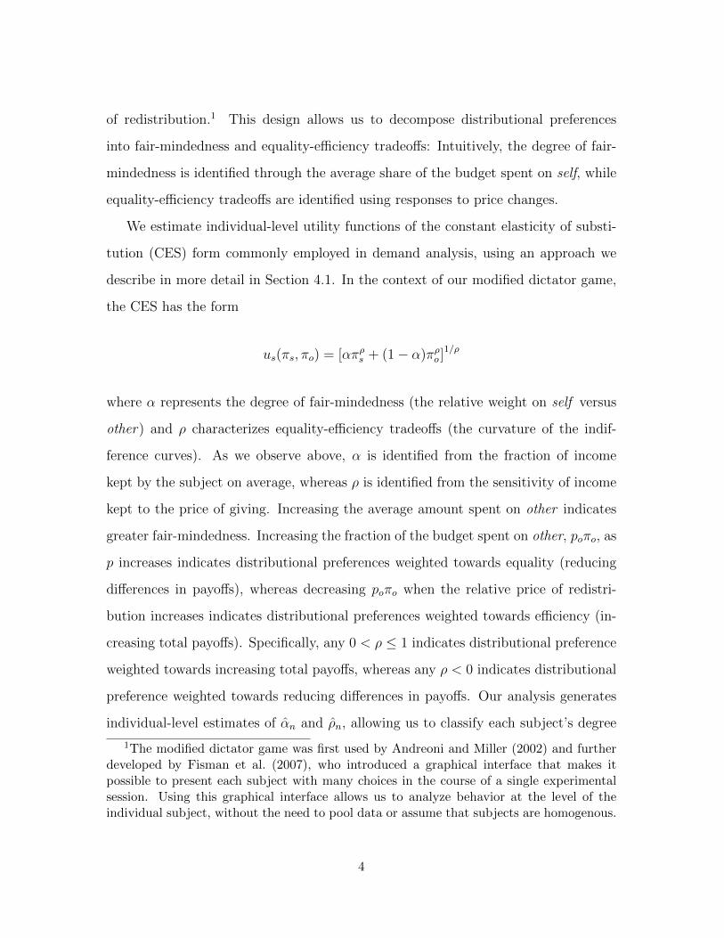
of redistribution.1 This design allows us to decompose distributional preferences

into fair-mindedness and equality-efficiency tradeoffs: Intuitively, the degree of fair-

mindedness is identified through the average share of the budget spent on self, while

equality-efficiency tradeoffs are identified using responses to price changes.

We estimate individual-level utility functions of the constant elasticity of substi-

tution (CES) form commonly employed in demand analysis, using an approach we

describe in more detail in Section 4.1. In the context of our modified dictator game,

the CES has the form

us(πs, πo) = [απρs + (1− α)πρo ]1/ρ

where α represents the degree of fair-mindedness (the relative weight on self versus

other) and ρ characterizes equality-efficiency tradeoffs (the curvature of the indif-

ference curves). As we observe above, α is identified from the fraction of income

kept by the subject on average, whereas ρ is identified from the sensitivity of income

kept to the price of giving. Increasing the average amount spent on other indicates

greater fair-mindedness. Increasing the fraction of the budget spent on other, poπo, as

p increases indicates distributional preferences weighted towards equality (reducing

differences in payoffs), whereas decreasing poπo when the relative price of redistri-

bution increases indicates distributional preferences weighted towards efficiency (in-

creasing total payoffs). Specifically, any 0 < ρ ≤ 1 indicates distributional preference

weighted towards increasing total payoffs, whereas any ρ < 0 indicates distributional

preference weighted towards reducing differences in payoffs. Our analysis generates

individual-level estimates of αn and ρn, allowing us to classify each subject’s degree

1The modified dictator game was first used by Andreoni and Miller (2002) and furtherdeveloped by Fisman et al. (2007), who introduced a graphical interface that makes itpossible to present each subject with many choices in the course of a single experimentalsession. Using this graphical interface allows us to analyze behavior at the level of theindividual subject, without the need to pool data or assume that subjects are homogenous.

4

of fair-mindedness and equality-efficiency tradeoffs.

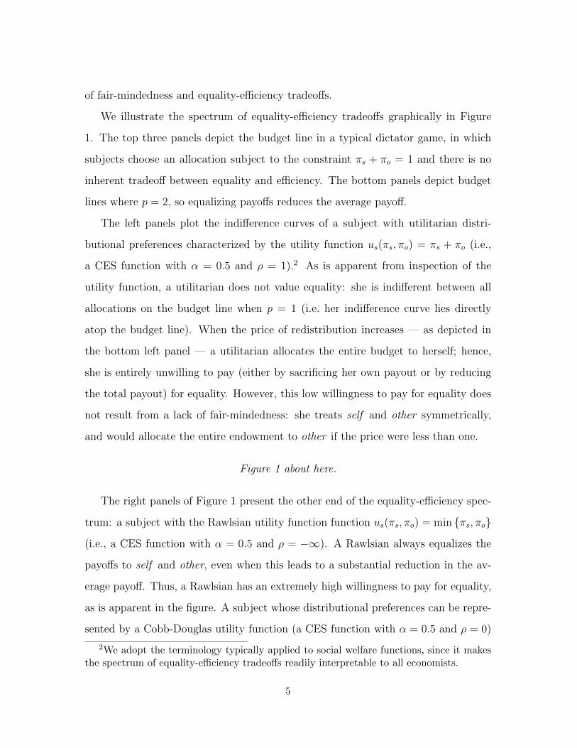
We illustrate the spectrum of equality-efficiency tradeoffs graphically in Figure

1. The top three panels depict the budget line in a typical dictator game, in which

subjects choose an allocation subject to the constraint πs + πo = 1 and there is no

inherent tradeoff between equality and efficiency. The bottom panels depict budget

lines where p = 2, so equalizing payoffs reduces the average payoff.

The left panels plot the indifference curves of a subject with utilitarian distri-

butional preferences characterized by the utility function us(πs, πo) = πs + πo (i.e.,

a CES function with α = 0.5 and ρ = 1).2 As is apparent from inspection of the

utility function, a utilitarian does not value equality: she is indifferent between all

allocations on the budget line when p = 1 (i.e. her indifference curve lies directly

atop the budget line). When the price of redistribution increases — as depicted in

the bottom left panel — a utilitarian allocates the entire budget to herself; hence,

she is entirely unwilling to pay (either by sacrificing her own payout or by reducing

the total payout) for equality. However, this low willingness to pay for equality does

not result from a lack of fair-mindedness: she treats self and other symmetrically,

and would allocate the entire endowment to other if the price were less than one.

Figure 1 about here.

The right panels of Figure 1 present the other end of the equality-efficiency spec-

trum: a subject with the Rawlsian utility function function us(πs, πo) = min {πs, πo}

(i.e., a CES function with α = 0.5 and ρ = −∞). A Rawlsian always equalizes the

payoffs to self and other, even when this leads to a substantial reduction in the av-

erage payoff. Thus, a Rawlsian has an extremely high willingness to pay for equality,

as is apparent in the figure. A subject whose distributional preferences can be repre-

sented by a Cobb-Douglas utility function (a CES function with α = 0.5 and ρ = 0)

2We adopt the terminology typically applied to social welfare functions, since it makesthe spectrum of equality-efficiency tradeoffs readily interpretable to all economists.

5

— shown in the middle panels of Figure 1 — falls in between the two extremes.

By estimating individual-level distributional preference parameters in a broad

sample of voting-age Americans, we are able to show that Americans are heteroge-

neous in terms of both fair-mindedness and equality-efficiency tradeoffs. Our main

analysis then focuses on the relationship between political decisions and distributional

preferences, as captured by estimated CES parameters. Consistent with preferences

over equality-efficiency tradeoffs influencing political decisions, we find that ρn is neg-

atively related to the probability of having voted for Barack Obama in 2012 and also

negatively related to the probability of reporting an affiliation with the Democratic

Party. By contrast, we do not find a significant relationship between our experimental

measure of fair-mindedness, αn, and either voting behavior or party affiliation; nor

do we find that less fair-minded individuals from low (resp. high) income households

are more likely to affiliate with the Democrats (resp. Republicans).3

Our findings contribute to our understanding of the determinants of political pref-

erences. While political platforms are multidimensional and the determinants of voter

support both complex and multifaceted, we show that underlying equality-efficiency

tradeoffs of voters are a potentially important input into individuals’ political alle-

giances. Our particular focus on distributional preferences may also yield insights into

the link between voter preferences and tax policy outcomes. As Saez and Stantcheva

(2013) emphasize, optimal tax policy will depend on the distributional preferences

of voters and taxpayers, and our work provides a first step in characterizing these

preferences. Our design is particularly well-suited to this task, as each subject makes

tradeoffs between her own payoff and the payoff an individual drawn from the general

population of the U.S. (another ALP respondent). This stands in contrast to many

experiments, in which subjects are generally matched with someone from their own

3Because our measure of household income provides only a rough indicator of the likelybeneficiaries of government redistribution, we do not view our results as evidence thatself-interest plays no role in political decisions.

6

community. Further, our experimentally generated measure of distributional prefer-

ences is not confounded by subjects’ attitudes toward government in general, as is

the case for survey-based measures of distributional preferences based on attitudes

toward government redistribution (Saez and Stantcheva 2013).

2 Related Literature

Experimental research has been very fruitful in documenting the existence of (non-

selfish) distributional preferences and directing theoretical attention toward such pref-

erences. We will not attempt to review the large and growing body of research on

the topic. Key contributions include Loewenstein, Thompson and Bazerman (1989),

Bolton (1991), Rabin (1993), Levine (1998), Fehr and Schmidt (1999), Bolton and

Ockenfels (1998, 2000), Charness and Rabin (2002, 2005), and Andreoni and Miller

(2002) among others. Camerer (2003) and Cooper and Kagel (2015) provide a com-

prehensive discussion of the experimental and theoretical work in economics. The

overarching lesson from hundreds of experiments is that people often sacrifice their

own payoffs in order to increase the payoffs of (unknown) others, and they do so even

in circumstances that do not engage reciprocity motivations or strategic considera-

tions.

Andreoni and Miller (2002) first proposed varying the price of redistribution

within a dictator game to identify equality-efficiency tradeoffs. Fisman et al. (2007)

extend their modified dictator game by introducing an experimental technique (a

graphical computer interface) that allows for the collection of richer individual-level

data from dictator game experiments than had previously been possible. This is par-

ticularly important given that, as Andreoni and Miller (2002) emphasize, individual

preferences are heterogeneous, so behavior must be examined at the individual level

7

for distributional preferences to be properly understood.4

Our paper contributes to several related literatures. We follow in the tradition

of other distributional preference experiments that have used subjects drawn from

broad cross-sections of the adult population (as opposed to university students).

Bellemare, Kroger and van Soest (2008) study distributional preferences in a large

and heterogeneous sample of Dutch adults. In their experiment, survey respondents

from the CentERpanel participate in ultimatum games. Like the ALP, the Cen-

tERpanel implements sophisticated experiments and collects extensive demographic

and economic information from its members. Data characterizing subjects’ decisions

within the experiment, their beliefs about the likelihood that specific ultimatum game

offers would be accepted, and their individual characteristics are used to estimate a

structural model of inequality aversion (Fehr and Schmidt 1999) in the Dutch pop-

ulation. In our analysis, we restrict attention to dictator games, which allows us to

focus on behavior motivated by purely distributional preferences and thus ignore the

complications of strategic behavior and reciprocity motivations inherent in response

games.5 Furthermore, our focus is on the link between distributional preferences

(both fair-mindedness and equality-efficiency tradeoffs) measured in the laboratory

and political decisions in the real world, with the aim of enriching models of voting

4Hong, Ding and Yao (2015) extend this work along another dimension, examining howsocial planners divide an endowment between two anonymous others in a generalized dicta-tor game, and further explore the correlates of equality-efficiency tradeoffs in their subjectpool of students at Chinese universities. Fisman, Jakiela, Kariv and Markovits (2015b)demonstrate the predictive validity of the preference parameters elicited using Fisman etal.’s (2007) graphical dictator game interface by showing that our experimental measureof equality-efficiency tradeoffs predicts the subsequent career choices of Yale Law Schoolstudents — more efficiency-focused students are more likely choose careers in corporate law,while more equality-focused students are more likely to work in the non-profit sector. Inrelated work, Fisman, Jakiela and Kariv (2015a) use the same experimental methodologyto estimate the impact of the Great Recession on distributional preferences.

5Our experimental design also allows us to generate individual-level estimates of dis-tributional preferences, which allows us to avoid making restrictive assumptions aboutindividuals’ utility functions and the distribution of unobserved heterogeneity within thepopulation.

8

and/or political competition. Given our sample of American subjects, we also hope

to add to our understanding of redistributive policy formation in the U.S.

Additionally, our experimental findings contribute to a literature that documents

and analyzes non-pecuniary motives for redistribution, employing theory and survey

survey evidence. Alesina and Angeletos (2005), for example, observe that attitudes

toward fairness of redistribution and observed redistributive policies may co-evolve

as an equilibrium, whereas in the model of Corneo and Gruner (2000) preferences

for redistribution are dictated by social comparisons. Survey-based and experimen-

tal evidence finds support for these theories, for example in Corneo and Gruner

(2002), which shows that social comparison and public-mindedness (as well as selfish

concerns) are determinants of redistributive preferences. Fong (2001) similarly find

that a standard model of self-interest fails to explain patterns in the redistributive

preferences of Americans. In a similar spirit, Corneo and Fong (2008) shows using

survey data that subjects are willing sacrifice their own income to see a just income

distribution.

Finally, like Bellemare et al. (2008, 2011), our work also contributes to the rapidly

expanding literature characterizing the distributional preferences of the general (non-

student) population. Much of this work focuses on cross-country differences in distri-

butional preferences; seminal contributions include Roth, Prasnikar, Okuno-Fujiwara

and Zamir (1991), Henrich, McElreath, Barr, Ensminger, Barrett, Bolyanatz, Carde-

nas, Gurven, Gwako, Henrich, Lesorogol, Marlowe, Tracer and Ziker (2006), and Hen-

rich, Ensminger, McElreath, Barr, Barrett, Bolyanatz, Cardenas, Gurven, Gwako,

Henrich, Lesorogol, Marlowe, Tracer and Ziker (2010). Our work is most closely

related to papers such as Hermann, Thoni and Gachter (2008) that explore the con-

nections between the distributional preferences of a population and political economic

outcomes within that country.

9

3 Experimental Design

3.1 Subject Pool

We embed an incentivized experiment in the American Life Panel (ALP), an internet

survey administered by the RAND Corporation to more than 5,000 adult Americans.6

To recruit subjects for our experiment, ALP administrators sent email invitations to

a random sample of ALP respondents in September of 2013. 1,172 ALP respondents

received the email and logged in to the experiment.7 Of those, 1,043 (89.9 percent)

progressed to the incentivized decision problems and 1,002 respondents (85.5 percent)

completed the entire experiment; these subjects constitute our subject pool.8

Subjects in our experiment are from 47 U.S. states, and range in age from 19

to 91. 58 percent are female. 9 percent of our subjects did not finish high school,

6ALP respondents have been recruited in several different ways, including from repre-sentative samples of the U.S. population. The initial participants were selected from theMonthly Survey Sample of the University of Michigan’s Survey Research Center. Additionalrespondents have been added through random digit dialling, targeted recruitment of a vul-nerable population sample of low-income individuals, and snowball sampling of existingpanel members. See the ALP website (https://mmicdata.rand.org/alp/) for informationon panel composition, demographics, attrition and response rates, sampling weights, and acomparison with other data sources.

7Those ALP respondents for whom complete demographic information was unavailablewere not eligible to participate. ALP administrators sent email invitations to a randomsample of 1,700 respondents (out of approximately 4,000) for whom a valid email addressand complete demographic information was available. We are unable to distinguish subjectswho read the invitation email and chose not to participate from those who never received theinvitation (for example, because they do not regularly access the email account registeredwith the ALP).

8The composition of the un-weighted ALP subject pool differs from the U.S. population(as is typical in all surveys based on random samples). In the Online Appendix, we compareour experimental subjects to both the (un-weighted) ALP sample and to the AmericanCommunity Survey (ACS) conducted by the U.S. Census and representative of the U.S.population in 2012. Like the U.S. population, both our subject pool and the ALP databaseincludes an enormous amount of demographic, socioeconomic, and geographic diversity;moreover, the subsample of 1,002 ALP respondents that constitute our subject pool isremarkably consistent with the entire ALP sample. Throughout our analysis, we re-weightour sample to be representative of the U.S. (adult) population in terms of gender, age,race/ethnicity, and educational attainment.

10

while 31 percent hold college degrees. 56 percent of subjects are currently employed;

the remainder include retirees (17 percent), the unemployed (11 percent), the dis-

abled (8 percent), homemakers (6 percent), and others who are on medical leave or

otherwise temporarily absent from the workforce. 68 percent identify themselves as

non-Hispanic whites, 18 percent as Hispanic or Latino, and 11 percent as African

American. 18 percent live in the Northeast (census region I), 20 percent in the Mid-

west (census region II), 35 percent in the South (census region III), and 267 percent in

the West (census region IV). Our subject pool therefore contains under-represented

groups in terms of age, educational attainment, household income, occupational sta-

tus, and place of residence. As discussed above, all of our results are weighted to

be representative of the U.S. population in terms of gender, age, race/ethnicity, and

educational attainment, though un-weighted results are nearly identical because the

differences between our subject pool and the general population are relatively minor.9

3.2 Experimental Procedures

To provide a positive account of individual distributional preferences, one needs a

choice environment that is rich enough to allow a general characterization of patterns

of behavior; Fisman et al. (2007) developed a computer interface for exactly this

purpose. The interface presents a standard consumer decision problem as a graphical

representation of a budget line and allows the subject to make choices using a simple

point-and-click tool.10

In this paper, we study a modified dictator game in which a subject divides an

9Un-weighted results are reported in Fisman, Jakiela and Kariv (2014).10The experimental method is applicable to many types of individual choice problems.

See Choi, Fisman, Gale and Kariv (2007) and Ahn, Choi, Gale and Kariv (2014), forsettings involving, respectively, risk and ambiguity. Choi, Kariv, Muller and Silverman(2014) investigate the correlation between individual behavior under risk and demographicand economic characteristics within the CentERpanel, a representative sample of more than2,000 Dutch households; that project demonstrated the feasibility of using the graphicalexperimental interface in web-based surveys.

11

endowment between self and an anonymous other, an individual chosen at random

from among the ALP respondents not sampled for the experiment. The subject

is free to allocate a unit endowment in any way she wishes subject to the budget

constraint, psπs + poπo = 1, where πs and πo denote the payoffs to self and other,

respectively, and p = po/ps is the relative price of redistribution. This decision

problem is presented graphically on a computer screen, and the subject must choose

a payoff allocation, (πs, πo), from a budget line representing feasible payoffs to self and

other. Responses to price changes allow us to identify equality-efficiency tradeoffs. A

subject who increases the fraction of the budget spent on other as the relative price

of redistribution increases has preferences weighted towards equality (i.e. minimizing

differences in payoffs), while a subject who decreases the fraction of the budget spent

on other as the relative price of redistribution increases has preferences weighted

towards efficiency (maximizing the aggregate payoff).11

The experiment consisted of 50 independent decision problems. For each decision

problem, the computer program selected a budget line at random from the set of lines

that intersect at least one of the axes at 50 or more experimental currency tokens,

but with no intercept exceeding 100 tokens. Subjects made their choices by using the

computer mouse or keyboard arrows to move the pointer to the desired allocation,

(πs, πo), and then clicked the mouse or hit the enter key to confirm their choice.

At the end of the experiment, payoffs were determined as follows. The experi-

mental program first randomly selected one of the 50 decision problems to carry out

for real payoffs. Each decision problem had an equal probability of being chosen.

Each subject then received the tokens that she allocated to self in that round, πs,

while the randomly-chosen ALP respondent with whom she was matched received the

11In a standard dictator experiment (cf. Forsythe, Horowitz, Savin and Sefton 1994),πs + πo = 1: the set of feasible payoff pairs is the line with a slope of −1, so the problemis simply dividing a fixed total income between self and other, and there is no inherenttradeoff between equality and efficiency.

12

tokens that she allocated to other, πo.12 Payoffs were calculated in terms of tokens

and then translated into dollars at the end of the experiment. Each token was worth

50 cents. Subjects received their payments from the ALP reimbursement system via

direct deposit into a bank account. Full experimental instructions are included in the

Online Appendix.

4 Decomposing Distributional Preferences

The experiment allows us to analyze behavior at the level of individual subject, test-

ing whether choices are consistent with individual utility maximization and if so

identifying the structural properties of the underlying utility function, without the

need to pool data or assume that subjects are homogenous. If budget sets are lin-

ear (as in our experiment), classical revealed preference theory (Afriat 1967; Varian

1982, 1983) provides a direct test: choices in a finite collection of budget sets are

consistent with maximizing a well-behaved utility function if and only if they satisfy

the Generalized Axiom of Revealed Preference (GARP). To account for the possibil-

ity of errors, we assess how nearly individual choice behavior complies with GARP

by using Afriat’s (1972) Critical Cost Efficiency Index (CCEI). We find that most

subjects exhibit GARP violations that are minor enough to ignore for the purposes

12To describe preferences with precision at the individual level, it is necessary to generatemany observations per subject over a wide range of budget sets. Our subjects made decisionsover 50 budget sets, with one decision round selected at random from each subject to carryout for payoffs. This random selection approach is a standard practice, although it is thesubject of ongoing controversy in the literature. If we paid for all rounds, subjects couldeasily hedge against inequality. The random payoff method prevents such hedging andreveals underlying distributional preferences only under stringent independence conditions.However, hedging relies heavily on the fact that the individual knows the parameters offuture budget set. In our experiment, subjects faced a large menu of highly heterogeneousbudget sets, and were only informed about the price’s random generating process, makingit difficult to hedge. Finally, given the novelty of our experimental design, we wished tokeep as many aspects of the experiment consistent with prior studies as was possible. Therandom selection approach is the method used by Andreoni and Miller (2002), among manyothers.

13

of recovering distributional preferences or constructing appropriate utility functions.

To economize on space, the revealed preference analysis is provided in the Online

Appendix.

4.1 The CES Utility Specification

Our subjects’ CCEI scores are sufficiently close to one to justify treating the data as

utility-generated, and Afriat’s theorem tells us that the underlying utility function,

us(πs, πo), that rationalizes the data can be chosen to be increasing, continuous and

concave. In the case of two goods, consistency and budget balancedness imply that

demand functions must be homogeneous of degree zero. If we also assume separability

and homotheticity, then the underlying utility function, us(πs, πo), must be a member

of the constant elasticity of substitution (CES) family commonly employed in demand

analysis (see the introduction for the specific form of the CES in our setting).13 The

CES specification is very flexible, spanning a range of well-behaved utility functions

by means of the parameters α and ρ. The parameter α represents the weight on

payoffs to self versus other (fair-mindedness), while ρ parameterizes the curvature of

the indifference curves (equality-efficiency tradeoffs).

When α = 1/2, a subject is fair-minded in the sense that self and other are treated

symmetrically. Among fair-minded subjects, the family of CES utility functions

spans the spectrum from Rawlsianism to utilitarianism as ρ ranges from −∞ to 1.

In particular, as ρ approaches −∞, us(πs, πo) approaches min{πs, πo}, the maximin

utility function of a Rawlsian (illustrated in Figure 1); as ρ approaches 1, us(πs, πo)

approaches that of a utilitarian, πs+πo (also illustrated in Figure 1). Hence, both the

13The proper development of revealed preference methods to test whether data are con-sistent with a utility function with some special structure, particularly homotheticity andseparability, is beyond the scope of this paper. Varian (1982, 1983) provides combinatorialconditions that are necessary and sufficient for extending Afriat’s (1967) Theorem to testingfor special structure of utility, but these conditions are not simple adjustments of the usualtests, which are all computationally intensive for large datasets like our own.

14

Rawlsian and the utilitarian utility functions, as well as a whole class of intermediate

fair-minded utility functions, are admitted by the CES specification.

More generally, as we observed in the introduction, different values of ρ give dif-

ferent degrees to which equality is valued over efficiency. Any 0 < ρ ≤ 1 indicates

distributional preference weighted towards efficiency (increasing total payoffs) be-

cause the expenditure on the tokens given to other, poπo, decreases when the relative

price of giving p = po/ps increases, whereas any ρ < 0 indicates distributional prefer-

ence weighted toward equality (reducing differences in payoffs) because poπo increases

when p increases. As ρ approaches 0, us(πs, πo) approaches the Cobb-Douglas utility

function, παs π1−αo , so the expenditures on tokens to self and other are constant for

any price p — a share α is spent on tokens for self and a share 1 − α is spent on

tokens for other.14

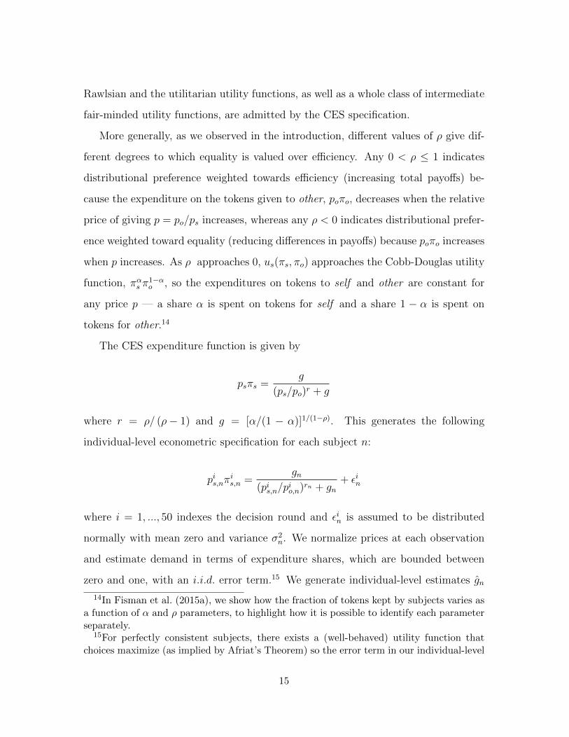
The CES expenditure function is given by

psπs =g

(ps/po)r + g

where r = ρ/ (ρ− 1) and g = [α/(1 − α)]1/(1−ρ). This generates the following

individual-level econometric specification for each subject n:

pis,nπis,n =

gn(pis,n/p

io,n)rn + gn

+ εin

where i = 1, ..., 50 indexes the decision round and εin is assumed to be distributed

normally with mean zero and variance σ2n. We normalize prices at each observation

and estimate demand in terms of expenditure shares, which are bounded between

zero and one, with an i.i.d. error term.15 We generate individual-level estimates gn

14In Fisman et al. (2015a), we show how the fraction of tokens kept by subjects varies asa function of α and ρ parameters, to highlight how it is possible to identify each parameterseparately.

15For perfectly consistent subjects, there exists a (well-behaved) utility function thatchoices maximize (as implied by Afriat’s Theorem) so the error term in our individual-level

15

and rn using non-linear Tobit maximum likelihood, and use these estimates to infer

the values of the underlying CES parameters αn and ρn.

To emphasize that α and ρ capture distinct — and largely independent — elements

to individuals’ distributional preferences, we observe that our estimates of individuals’

parameters are largely uncorrelated: the correlation between the deciles (to limit the

influence of outliers) of ρ and α is -0.06, a relationship that is virtually identical for

both subjects who voted for Obama (correlation of -0.05) and those who did not

(correlation of -0.07).

4.2 The Distributional Preferences of Americans

Table 1 provides a population-level summary of the parameter estimates. We classify

subject n as fair-minded if αn is between 0.45 and 0.55; we classify subject n as

selfish if αn > 0.95.16 Using this criterion, we estimate that 30.9 percent of the U.S.

population is fair-minded, while only 16.7 percent is selfish (αn > 0.95). Thus, fair-

minded subjects outnumber selfish ones by approximately 2 to 1. We estimate that

58.8 percent of the U.S. population is equality-focused, having ρn < 0. However, a

relatively small proportion of the population (only 12.6 percent) is both fair-minded

and equality-focused: fair-minded subjects are less likely to be equality-focused than

than those whose estimated αn parameters characterize them as either selfish or

intermediate (0.55 < αn < 0.95).

Table 1 about here.

Exploiting the detailed demographic and economic data available on ALP sub-

regression analysis can only stem from misspecifications of the functional form. For less thanperfectly consistent subjects, the error term also captures the fact these subjects computeincorrectly, execute intended choices incorrectly, or err in other ways. Disentangling thesesources of noise is beyond the scope of this paper.

16We obtain similar results using other thresholds to identify subjects’ types, or if weuse statistical tests to classify types. CDFs of the estimated preference parameters arepresented in the Online Appendix.

16

jects, we examine the correlates of the estimated αn and ρn parameters in a regression

framework. OLS estimates (reported in the Online Appendix) suggest that African

Americans are more fair-minded than the rest of the sample; however, the association

is not statistically significant after implementing a correction for the false discovery

rate (which is necessary because we consider a wide range of demographic and so-

cioeconomic factors that might be associated with the degree of fair-mindedness).17

Turning to our estimated ρn parameters, we find that younger people, employed peo-

ple, and those from lower-income households display greater efficiency focus, while

women show greater equality focus. However, after implementing the multiple test

correction, only the association with age remains statistically significant at conven-

tional levels (Benjamini-Hochberg q-value 0.010).18

While observable attributes have predictive power in the data, we find that marked

heterogeneity in distributional preferences remains within each demographic and eco-

nomic group: observable attributes explain only about four percent of the variation

in CES parameters. Thus, though some groups appear more efficiency-focused than

others, these between-group differences are modest relative to the tremendous vari-

ation in efficiency orientation within the demographic and socioeconomic categories

in our sample.

17In the Online Appendix, we report OLS coefficients and standard errors from regres-sions of the CES parameters, αn and ρn, on 16 different demographic and socioeconomiccharacteristics. We also report Benjamini-Hochberg q-values, which correct for the falsediscovery rate (Benjamini and Hochberg 1995, Anderson 2008).

18The q-values associated with the other three variables are all reasonably close tomarginal significance, however. The Benjamini-Hochberg q-value associated with both thefemale indicator and the indicator for coming from a lower-income household is 0.109. Theq-value associated with the indicator for being employed is 0.116.

17

5 Distributional Preferences and Political Behavior

Turning now to our main analysis, we test whether distributional preferences, as

measured in our experiment, predict support for political candidates who favor re-

distribution. We explore the link between equality-efficiency tradeoffs and political

behavior by looking at voting decisions in the 2012 presidential election.19 Our main

dependent variable is an indicator for voting for Democrat Barack Obama, a relatively

pro-redistribution party and candidate, rather than Republican Mitt Romney. We

focus on the 766 subjects who participated in ALP modules exploring participants’

choices in the 2012 election and who report voting for either Barack Obama or Mitt

Romney, re-weighted to be representative of the United States population in terms

of gender, age, race/ethnicity, and educational attainment.20 We include a range of

demographic controls to account for the fact that, for example, African Americans

overwhelmingly voted for Obama for reasons that are plausibly distinct from their

distributional preferences. Interestingly, without controls, the relationship between

measured distributional preferences and voting is insignificant in all regressions, re-

flecting the fact that groups such as African Americans and low income individuals

tend to support Democratic candidates, but are also more efficiency-focused in our

experiments. We employ a linear probability model with an indicator variable for

having voted for Obama as the outcome.21 Since the distribution of ρn is highly

skewed, we report results for three measures of equality-efficiency tradeoffs: the es-

timated ρn parameter; ρn deciles; and ρhigh, an indicator for being efficiency-focused

19Data on voting behavior in the 2008 election is not available for most of our subjects,in part because the ALP sample is regularly refreshed with new respondents, and becausemost studies recruit only a small fraction of ALP respondents (so the overlap between ourrandomly-chosen subjects and those who participated in other studies is limited).

20Unfortunately, no information is available on the voting behavior of the 48 subjectswho participated in the relevant ALP survey module but did not report casting a ballotfor a major party candidate, so we cannot classify the candidates that they supported asbeing either for or against redistribution.

21Probit results are nearly identical.

18

in the sense of having an estimated ρn of at least 0.

In the first three columns of Table 2, we present specifications that include demo-

graphic controls and state fixed effects, showing results for each of the three trans-

formations of ρn.22 In all three specifications, the experimentally-elicited measure

of equality-efficiency tradeoffs is statistically significant, indicating that efficiency-

focused subjects are less likely to have voted for Barack Obama. The most straight-

forward coefficient to interpret is that on ρhigh in Column 3, which indicates that

efficiency-focused subjects (with ρn ≥ 0) are 7 percentage points less likely to have

voted for Obama than Romney. To provide a benchmark for the magnitude of this

effect, we include (in the Online Appendix) the full set of regression coefficients from

specifications with and without the inclusion of ρhigh as a covariate. We observe, for

example, that the impact of ρhigh is greater than the effect of gender (0.044), and

only marginally smaller than the impact of moving from medium to high income

(−0.102). It is also of note that the coefficient on female declines somewhat with

the inclusion of ρhigh, indicating that some amount of the gender voting gap can be

directly accounted for by distributional preferences.

Table 2 about here.

In Columns 4 through 6 we repeat our analyses while controlling for the degree

of fair-mindedness. Results are nearly identical: efficiency-focused subjects are sig-

nificantly less likely to have voted for Barack Obama in 2012. Moreover, we do not

observe an association between the degree of fair-mindedness and the likelihood of

voting for Obama. In Panel B of Table 2, we omit nearly selfish subjects who allocate

an average of more than 99 percent of the tokens to self because estimates of ρn are

22As expected, including state fixed effects increases power substantially. Results aredirectionally similar but not consistently significant when state fixed effects are omitted.Results are similar in magnitude and significance when standard errors are clustered at thestate level.

19

quite noisy for these individuals. As expected, reducing the level of measurement er-

ror in the independent variable of interest generates estimates that are slightly larger

in magnitude, leading to marginally higher levels of statistical significance across all

specifications.

We further explore the relationship between equality-efficiency tradeoffs and po-

litical behavior by replicating our specifications using an indicator for alignment

with the Democratic Party as an outcome variable. These specifications include 528

subjects who participated in ALP modules on politics and identified themselves as

either Republicans or Democrats.23 We report our results in Table 3. All estimated

coefficients on ρn and its transformations are negative and (at least marginally) sta-

tistically significant, suggesting that more efficiency-focused subjects are less likely to

be Democrats. After controlling for individual characteristics and geographic fixed

effects, the estimated coefficient on ρhigh suggests that efficiency-focused subjects are

11.0 percentage points less likely to be Democrats. We again provide the full set of

regression coefficients in the Online Appendix, both with and without ρhigh as a co-

variate. For the dependent variable of Democrat, the impact of ρn is large relative

to other covariates.

Table 3 about here.

Overall, our results strongly suggest that the political decisions of Americans are

motivated by their equality-efficiency preferences, and not just their own self-interest

or their views of government. However, this pattern only emerges after one accounts

for the fact that poorer Americans and minorities are, overall, substantially more

focused on efficiency than the rest of the population.

23Results are similar when we include the 217 additional subjects who participated in thepolitics module and identified themselves as Independents. 55 subjects participated in themodule but indicated their party affiliation as “other,” so their parties cannot be classifiedas more or less equality-focused than the Democrats.

20

In our final piece of analysis, we explore the relationship between fair-mindedness

and political behavior, paralleling our analysis of the link between equality-efficiency

tradeoffs and political preferences. Results are reported in Table 4. We first test

whether relatively more fair-minded Americans are inclined to support candidates

who favor greater redistribution. Across all specifications, we find no significant rela-

tionship between our experimental measure of fair-mindedness, αn, and either voting

behavior or party affiliation across all specifications. This insignificant effect could

be masking the opposing effects of self-interest on voting behavior for different sub-

populations: a self-interested low-income individual should favor Democrats, while

the opposite should be the case for a self-interested high-income individual.24 Inter-

estingly, we do not find support for this view in the data: the correlation between

fair-mindedness and political preferences does not differ significantly by subject in-

come. This suggests that Americans may not vote for redistributive policies purely

out of (monetary) self-interest.25

Table 4 about here.

6 Conclusion

In this paper, we analyze the relationship between experimentally-derived measures

of social preferences and political decisions. In our main analysis, which takes into

account the fact that poorer Americans and minorities are substantially more focused

24An extensive literature explores the extent to which voters support policies that are intheir own perceived short-run and long-run economic interests. See, Alesina and La Ferrara(2005) and the references cited therein.

25Prior work, for example Fong and Oberholzer-Gee (2011), also emphasizes that giving indictator games is influenced by the income of the recipient. Differences in fair-mindednessbetween Republicans and Democrats may have emerged if our experiment involved low-income subjects because of different notions of deservingness of the poor (Gilens 2009).While our experiment is not designed to detect such differences, we also believe it reflectsan element of distributional preferences that is distinct from fair-mindedness, i.e., the sym-metric treatment of self and a comparable other.

21

on efficiency overall, we find that efficiency-equality tradeoffs predict support for

Republican candidate Mitt Romney in the 2012 election. Our results thus provide

a link from underlying distributional preferences to voter preferences over policy

outcomes. These results emphasize that individuals may not, as in the standard

median voter model, vote for redistributive policies that serve their own interests,

but may in fact have preferences over the income distribution itself.

Our findings may thus be useful in providing a positive explanation of public

support for policy issues related to redistribution. Most standard models of self-

interested political preferences predict that the increase in income inequality observed

in the United States over the last few decades should have led to greater support for

government redistribution. However, no such shift has been observed in survey data

(Kuziemko, Norton, Saez and Stantcheva 2013). Our findings partially explain this:

voters are motivated by their distributional preferences, so they may not vote for

redistributive policies which would make them better off individually.26

26Redistributive decisions depend on recipient attributes, and in particular ought to bea function of recipient income. In other work-in-progress, we study how distributionalpreferences vary based on the income of other, and with the degree of inequality betweenself and other. Introducing information about actual incomes into our experimental setup isperhaps the most important step toward understanding the distributional preferences mostrelevant to policy preferences and voting behavior, simply because views about how muchincome ought to be redistributed depend crucially on the initial incomes of the potentialrecipients of redistribution.

22

References

Afriat, Sydney N., “The Construction of Utility Functions from Expenditure

Data,” International Economic Review, 1967, 8 (1), 67–77.

, “Efficiency Estimates of Production Functions,” International Economic Re-

view, 1972, 8, 568–598.

Ahn, David, Syngjoo Choi, Douglas Gale, and Shachar Kariv, “Estimating

Ambiguity Aversion in a Portfolio Choice Experiment,” Quantitative Economics,

2014, 5 (2), 195–223.

Alesina, Alberto and Eliana La Ferrara, “Preferences for Redistribution in the

Land of Opportunities,” Journal of Public Economics, 2005, 89 (5), 897–931.

and George-Marios Angeletos, “Fairness and redistribution,” The American

Economic Review, 2005, 95 (4), 960–980.

Anderson, Michael L., “Multiple Inference and Gender Differences in the Effects

of Early Intervention: A Reevaluation of the Abecedarian, Perry Preschool, and

Early Training Projects,” Journal of the American Statistical Association, 2008,

103 (484), 1481–1495.

Andreoni, James and John Miller, “Giving According to GARP: An Experimen-

tal Test of the Consistency of Preferences for Altruism,” Econometrica, 2002, 70

(2), 737–753.

Becker, Gary S, “Irrational Behavior and Economic Theory,” The Journal of Po-

litical Economy, 1962, 70 (1), 1–13.

Bellemare, Charles, Sabine Kroger, and Arthur van Soest, “Measuring In-

equity Aversion in a Heterogeneous Population Using Experimental Decisions

and Subjective Probabilities,” Econometrica, 2008, 76 (4), 815–839.

23

, , and , “Preferences, Intentions, and Expectation Violations: A

Large-Scale Experiment with a Representative Subject Pool,” Journal of Eco-

nomic Behavior and Organization, 2011, 78 (3), 349–365.

Benjamini, Yoav and Yosef Hochberg, “Controlling the False Discovery Rate:

a Practical and Powerful Approach to Multiple Testing,” Journal of the Royal

Statistical Society. Series B (Methodological), 1995, 57 (1), 289–300.

Bolton, Gary E, “A Comparative Model of Bargaining: Theory and Evidence,”

The American Economic Review, 1991, pp. 1096–1136.

and Axel Ockenfels, “Strategy and Equity: an ERC-Analysis of the Guth–van

Damme Game,” Journal of Mathematical Psychology, 1998, 42 (2), 215–226.

and , “ERC: A Theory of Equity, Reciprocity, and Competition,” Ameri-

can Economic Review, 2000, pp. 166–193.

Bronars, Stephen G, “The Power of Nonparametric Tests of Preference Maximiza-

tion,” Econometrica, 1987, 55 (3), 693–698.

Camerer, Colin, Behavioral Game Theory, Princeton, NJ: Princeton University

Press, 2003.

Charness, Gary and Matthew Rabin, “Understanding Social Preferences with

Simple Tests,” Quarterly Journal of Economics, 2002, 117 (3), 817–869.

and , “Expressed Preferences and Behavior in Experimental Games,”

Games and Economic Behavior, 2005, 53 (2), 151–169.

Choi, Syngjoo, Raymond Fisman, Douglas Gale, and Shachar Kariv, “Con-

sistency and Heterogeneity of Individual Behavior under Uncertainty,” American

Economic Review, 2007, 97 (5), 1921–1938.

24

, Shachar Kariv, Wieland Muller, and Dan Silverman, “Who Is (More)

Rational?,” American Economic Review, 2014, 104 (6), 1518–1550.

Cooper, David and John H. Kagel, “Other regarding preferences: a selective

survey of experimental results,” in John H. Kagel and Alvin E. Roth, eds., Hand-

book of Experimental Economics Volume 2, Princeton, NJ: Princeton University

Press, 2015.

Corneo, Giacomo and Christina M Fong, “What’s the monetary value of dis-

tributive justice?,” Journal of Public Economics, 2008, 92 (1), 289–308.

and Hans Peter Gruner, “Social limits to redistribution,” The American

Economic Review, 2000, 90 (5), 1491–1507.

and , “Individual preferences for political redistribution,” Journal of public

Economics, 2002, 83 (1), 83–107.

Fehr, Ernst and Klaus M. Schmidt, “A Theory Of Fairness, Competition, and

Cooperation,” Quarterly Journal of Economics, 1999, 114 (3), 817–868.

Fisman, Raymond, Pamela Jakiela, and Shachar Kariv, “The Distributional

Preferences of Americans,” NBER Working Paper No. 20145 2014.

, , and , “How Did Distributional Preferences Change During the

Great Recession?,” Journal of Public Economics, 2015, 128, 84–95.

, , , and Daniel Markovits, “The Distributional Preferences of an

Elite,” Science, 2015, 349 (6254), aab0096.

, Shachar Kariv, and Daniel Markovits, “Individual Preferences for Giv-

ing,” American Economic Review, 2007, 97 (5), 1858–1876.

Fong, Christina, “Social Preferences, Self-Interest, and the Demand for Redistri-

bution,” Journal of Public Economics, 2001, 82 (2), 225–246.

25

Fong, Christina M and Felix Oberholzer-Gee, “Truth in giving: Experimental

evidence on the welfare effects of informed giving to the poor,” Journal of Public

Economics, 2011, 95 (5), 436–444.

Forsythe, Robert, Joel Horowitz, N. S. Savin, and Martin Sefton, “Fairness

in Simple Bargaining Games,” Games and Economic Behavior, 1994, 6 (3), 347–

369.

Gilens, Martin, Why Americans hate welfare: Race, media, and the politics of

antipoverty policy, University of Chicago Press, 2009.

Henrich, Joseph, Jean Ensminger, Richard McElreath, Abigail Barr, Clark

Barrett, Alexander Bolyanatz, Juan Camilo Cardenas, Michael Gur-

ven, Edwins Gwako, Natalie Henrich, Carolyn Lesorogol, Frank Mar-

lowe, David Tracer, and John Ziker, “Markets, Religion, Community Size,

and the Evolution of Fairness and Punishment,” Science, 2010, 327 (5972), 1480–

1484.

, Richard McElreath, Abigail Barr, Jean Ensminger, Clark Barrett,

Alexander Bolyanatz, Juan Camilo Cardenas, Michael Gurven, Ed-

wins Gwako, Natalie Henrich, Carolyn Lesorogol, Frank Marlowe,

David Tracer, and John Ziker, “Costly Punishment Across Human Soci-

eties,” Science, 2006, 312 (5781), 1767–1770.

Hermann, Benedikt, Christian Thoni, and Simon Gachter, “Antisocial Pun-

ishment Across Societies,” Science, 2008, 319 (5868), 1362–1367.

Hong, Hao, Jianfeng Ding, and Yang Yao, “Individual social welfare prefer-

ences: An experimental study,” Journal of Behavioral and Experimental Eco-

nomics, 2015, 57, 89–97.

26

Kuziemko, Ilyana, Michael I Norton, Emmanuel Saez, and Stefanie

Stantcheva, “How Elastic Are Preferences for Redistribution? Evidence from

Randomized Survey Experiments,” NBER Working Paper 18865, National Bu-

reau of Economic Research 2013.

Levine, David K., “Modeling Altruism and Spitefulness in Experiments,” Review

of Economic Dynamics, 1998, 1 (3), 593–622.

Loewenstein, George F, Leigh Thompson, and Max H Bazerman, “Social

Utility and Decision Making in Interpersonal Contexts,” Journal of Personality

and Social psychology, 1989, 57 (3), 426.

Rabin, Matthew, “Incorporating Fairness into Game Theory and Economics,” The

American economic review, 1993, pp. 1281–1302.

Roth, Alvin E., Vesna Prasnikar, Masahiro Okuno-Fujiwara, and Shmuel

Zamir, “Bargaining and Market Behavior in Jerusalem, Ljubljana, Pittsburgh,

and Tokyo: An Experimental Study,” American Economic Review, 1991, 81 (5),

1068–1095.

Saez, Emmanuel and Stefanie Stantcheva, “Generalized Social Marginal Wel-

fare Weights for Optimal Tax Theory,” Technical Report 18835, National Bureau

of Economic Research 2013.

Varian, Hal R., “The Nonparametric Approach to Demand Analysis,” Economet-

rica, 1982, 50 (4), 945–972.

, “Non-Parametric Tests of Consumer Behaviour,” Review of Economic Studies,

1983, 50 (1), 99–110.

27

Table 1: Classifying Distributional Preferences

Fair-Minded Intermediate Selfish All SubjectsEquality-Focused 12.6 35.4 10.8 58.8Efficiency-Focused 18.3 17.0 5.9 41.2All Subjects 30.9 52.4 16.7 100.0

The numbers indicate the percentage in each cell (weighted to be representative of the United States populationin terms of gender, age, race/ethnicity, and educational attainment). We classify a subject as fair-minded if0.45 < αn < 0.55; a subject is classified as selfish if αn > 0.95. We classify a subject as equality-focused(resp. efficiency-focused) if ρn < 0 (resp. ρn > 0). We obtain similar results using statistical tests to classifyindividual types.

28

Table 2: OLS Regressions of the Likelihood of Voting for Obama in 2012 on ρn

Specification: OLS OLS OLS OLS OLS OLS(1) (2) (3) (4) (5) (6)

Panel A: All Subjects

ρn -0.007∗∗ . . -0.007∗∗ . .(0.003) (0.003)

Decile of ρn . -0.014∗∗ . . -0.014∗∗ .(0.006) (0.006)

ρhigh (i.e. ρn ≥ 0) . . -0.07∗∗ . . -0.069∗

(0.035) (0.035)αn . . . 0.074 . .

(0.094)Decile of αn . . . . 0.002 0.001

(0.006) (0.006)Demographic Controls Yes Yes Yes Yes Yes YesState of Residence FEs Yes Yes Yes Yes Yes YesObservations 766 766 766 766 766 766

Panel B: Non-Selfish Subjects

ρn -0.007∗∗ . . -0.007∗∗ . .(0.003) (0.003)

Decile of ρn . -0.018∗∗∗ . . -0.018∗∗∗ .(0.006) (0.006)

ρhigh (i.e. ρn ≥ 0) . . -0.084∗∗ . . -0.088∗∗

(0.036) (0.037)αn . . . 0.015 . .

(0.097)Decile of αn . . . . -0.003 -0.004

(0.007) (0.007)Demographic Controls Yes Yes Yes Yes Yes YesState of Residence FEs Yes Yes Yes Yes Yes YesObservations 734 734 734 734 734 734

Robust standard errors in parentheses. Sample weighted to be representative of the United States populationin terms of gender, age, race/ethnicity, and educational attainment. Demographic controls are gender, age,race/ethnicity, education level, employment status, marital status, and religion (the specific variables includedin Tables A2 and A3 in the Online Appendix), plus controls for respondents who are missing data on race(2), household income (5), or religious affiliation (8).

29

Table 3: OLS Regressions of the Likelihood of Being a Democrat on ρn

Specification: OLS OLS OLS OLS OLS OLS(1) (2) (3) (4) (5) (6)

Panel A: All Subjects

ρn -0.006∗ . . -0.007∗ . .(0.003) (0.003)

Decile of ρn . -0.021∗∗∗ . . -0.021∗∗∗ .(0.008) (0.008)

ρhigh (i.e. ρn ≥ 0) . . -0.11∗∗ . . -0.108∗∗

(0.044) (0.045)αn . . . 0.077 . .

(0.119)Decile of αn . . . . 0.006 0.004

(0.008) (0.008)Demographic Controls Yes Yes Yes Yes Yes YesState of Residence FEs Yes Yes Yes Yes Yes YesObservations 528 528 528 528 528 528

Panel B: Non-Selfish Subjects

ρn -0.006∗ . . -0.006∗ . .(0.003) (0.003)

Decile of ρn . -0.025∗∗∗ . . -0.025∗∗∗ .(0.008) (0.008)

ρhigh (i.e. ρn ≥ 0) . . -0.126∗∗∗ . . -0.128∗∗∗

(0.046) (0.048)αn . . . 0.013 . .

(0.122)Decile of αn . . . . -0.001 -0.002

(0.008) (0.009)Demographic Controls Yes Yes Yes Yes Yes YesState of Residence FEs Yes Yes Yes Yes Yes YesObservations 505 505 505 505 505 505

Robust standard errors in parentheses. Sample weighted to be representative of the United States populationin terms of gender, age, race/ethnicity, and educational attainment. Demographic controls are gender, age,race/ethnicity, education level, employment status, marital status, and religion (the specific variables includedin Tables A2 and A3 in the Online Appendix), plus controls for respondents who are missing data on race(2), household income (5), or religious affiliation (8).

30

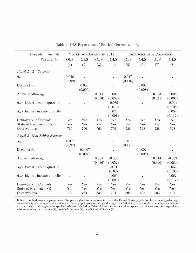
Table 4: OLS Regressions of Political Outcomes on αn

Dependent Variable: Voted for Obama in 2012 Identifies as a Democrat

Specification: OLS OLS OLS OLS OLS OLS OLS OLS

(1) (2) (3) (4) (5) (6) (7) (8)

Panel A: All Subjects

αn 0.046 . . . 0.047 . . .(0.092) (0.116)

Decile of αn . 0.003 . . . 0.006 . .(0.006) (0.008)

Above median αn . . 0.014 0.006 . . 0.023 0.008(0.036) (0.052) (0.045) (0.064)

αn× lowest income quartile . . . -0.039 . . . -0.001(0.079) (0.105)

αn× highest income quartile . . . 0.078 . . . 0.059(0.091) (0.112)

Demographic Controls Yes Yes Yes Yes Yes Yes Yes YesState of Residence FEs Yes Yes Yes Yes Yes Yes Yes YesObservations 766 766 766 766 528 528 528 528

Panel B: Non-Selfish Subjects

αn -0.008 . . . -0.011 . . .(0.097) (0.121)

Decile of αn . -0.0007 . . . 0.002 . .(0.007) (0.008)

Above median αn . . 0.004 -0.001 . . 0.014 -0.009(0.036) (0.052) (0.046) (0.064)

αn× lowest income quartile . . . -0.04 . . . 0.032(0.08) (0.106)

αn× highest income quartile . . . 0.069 . . . 0.062(0.094) (0.117)

Demographic Controls Yes Yes Yes Yes Yes Yes Yes YesState of Residence FEs Yes Yes Yes Yes Yes Yes Yes YesObservations 734 734 734 734 505 505 505 505

Robust standard errors in parentheses. Sample weighted to be representative of the United States population in terms of gender, age,race/ethnicity, and educational attainment. Demographic controls are gender, age, race/ethnicity, education level, employment status,marital status, and religion (the specific variables included in Tables A2 and A3 in the Online Appendix), plus controls for respondentswho are missing data on race (2), household income (5), or religious affiliation (8).

31

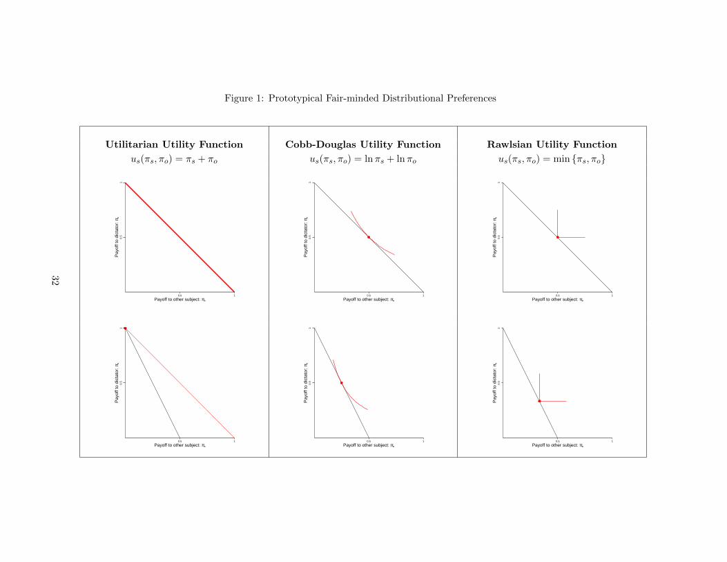
Figure 1: Prototypical Fair-minded Distributional Preferences

Utilitarian Utility Function Cobb-Douglas Utility Function Rawlsian Utility Function

us(πs, πo) = πs + πo us(πs, πo) = lnπs + lnπo us(πs, πo) = min {πs, πo}

0.5

1P

ayof

f to

dict

ator

: ps

0.5 1

Payoff to other subject: po

0.5

1P

ayof

f to

dict

ator

: ps

0.5 1

Payoff to other subject: po

0.5

1P

ayof

f to

dict

ator

: ps

0.5 1

Payoff to other subject: po

0.5

1P

ayof

f to

dict

ator

: ps

0.5 1

Payoff to other subject: po

0.5

1P

ayof

f to

dict

ator

: ps

0.5 1

Payoff to other subject: po

0.5

1P

ayof

f to

dict

ator

: ps

0.5 1

Payoff to other subject: po

32

Online Appendix: Not for Print Publication

A. Experimental Instructions

Welcome to this survey.

Login code:

Well Being 326 https://mmic.rand.org/research/rand/ms326/

1 of 1 8/5/2013 11:41 AM

33

Welcome.

Please remember: Participation in the survey is voluntary and you may skip over any questions that you wouldprefer not to answer. You will not be identified in any reports on this study.

Choose 'Next' to start the questionnaire.

Well Being 326 https://mmic.rand.org/research/rand/ms326/

1 of 1 8/5/2013 11:41 AM

34

This is an experiment in decision-making. Please pay careful attention to the instructions as a considerableamount of money is at stake.

During the experiment we will speak in terms of experimental tokens instead of dollars. Your payoffs will becalculated in terms of tokens and then translated into dollars at the end of the experiment at the following rate:

2 Tokens = 1 Dollar

You are free to stop at any time. If you do not complete the experiment now, you may return to complete theexperimental session at any time between now and 2013-08-15. If you do not complete the experiment betweennow and 2013-08-15, you will not receive any payment. Details of how you will make decisions and receivepayments will be provided below.

Please click the NEXT button below to proceed to the next screen.

Well Being 326 https://mmic.rand.org/research/rand/ms326/

1 of 1 8/5/2013 11:42 AM

35

In this experiment, you will make 50 decisions that share a common form. We next describe in detail the processthat will be repeated in all decision problems and the computer program that you will use to make your decisions.

In each decision, you will be asked to allocate tokens between yourself and another person who will be chosenat random from the group of American Life Panel (ALP) respondents who were not asked to participate in thisexperiment.

We will refer to the tokens that you allocate to yourself as tokens that you Hold, and tokens that you allocate tothe other person as tokens that you Pass to that individual. The identity of the ALP respondent who receives thetokens you pass depends entirely on chance.

Please click the NEXT button below to proceed to the next screen.

Well Being 326 https://mmic.rand.org/research/rand/ms326/

1 of 1 8/5/2013 11:42 AM

36

Each decision will involve choosing a point on a line representing possible token allocations to you (Hold) andthe other ALP respondent (Pass). In each decision, you may choose any combination of tokens to Hold andPass – in other words, any combination of tokens to yourself and tokens to the other ALP respondent – that is onthe line. Examples of lines that you might face appear in the diagrams below. In each graph, Hold correspondsto the vertical axis and Pass corresponds to the horizontal axis; the points on the diagonal lines in the graphsrepresent possible token allocations to Hold (tokens you to you) and Pass (tokens to the other ALP respondent)that you might choose.

Please click the NEXT button below to proceed to the next screen.

Well Being 326 https://mmic.rand.org/research/rand/ms326/

1 of 1 8/5/2013 11:42 AM

37

By picking a point on the diagonal line, you choose how many tokens to hold for yourself and how many to passto the other person. You may select any allocation to Hold and Pass on that line.

If, for example, the diagonal line runs from 50 tokens on the Hold axis to 50 tokens on the Pass axis (seeDiagram 4), you could choose to hold all 50 tokens for yourself, or pass all 50 tokens to the other person, oranything in between. However, most of the decision problems will involve flatter or steeper lines: if the line isflatter (see Diagram 5), one less token for yourself means more than one additional token is passed to the otherperson; if the line is steeper (see Diagram 6), one less token held means less than one additional token passedto the other person.

Please click the NEXT button below to proceed to the next screen.

Well Being 326 https://mmic.rand.org/research/rand/ms326/

1 of 1 8/5/2013 11:42 AM

38

To further illustrate, in the example below, choice A represents an allocation in which you hold y tokens and passx tokens. Thus, if you choose this allocation, you will hold y tokens for yourself and you will pass x tokens toanother person. Another possible allocation is B, in which you hold w tokens and pass z tokens to the otherperson.

Please click the NEXT button below to proceed to the next screen.

Well Being 326 https://mmic.rand.org/research/rand/ms326/

1 of 1 8/5/2013 11:42 AM

39

Each of the 50 decision problems will start by having the computer select a diagonal line at random. All of thelines that the computer will select will intersect with at least one of the axes at 50 or more tokens, but will notintersect either axis at more than 100 tokens. The lines selected for you in different decision problems areindependent of each other and depend solely upon chance.

Please click the NEXT button below to proceed to the next screen.

Well Being 326 https://mmic.rand.org/research/rand/ms326/

1 of 1 8/5/2013 11:42 AM

40

The computer programdialog window is shownhere. In each round, youwill choose an allocationby using the mouse tomove the pointer on thecomputer screen to theallocation that you wishto choose (note that thepointer does not need tobe precisely on thediagonal line to shift theallocation).

When you are ready tomake your decision, left-click to enter yourchosen allocation. Afterthat, confirm yourdecision by clicking onthe OK button. Note thatyou can choose onlyHold and Passcombinations that are onthe diagonal line. Onceyou have clicked the OKbutton, your decisioncannot be revised.

After you submit each choice, you will be asked to make another allocation in a different decision probleminvolving a different diagonal line representing possible allocations. Again, all decision problems areindependent of each other. This process will be repeated until all 50 decision rounds are completed. At the endof the last round, you will be informed that the experiment has ended.

Please click the NEXT button below to proceed to the next screen.

Well Being 326 https://mmic.rand.org/research/rand/ms326/

1 of 1 8/5/2013 11:43 AM

41

Next, you will have two practice decision rounds. The choices you make in these practice rounds will have noimpact on the final payoffs to you or to the other ALP respondent. In each round, you may choose anycombination of tokens to Hold (tokens to you) and Pass (tokens to the other ALP respondent) that are on theline. To choose an allocation, use the mouse to move the cursor on the computer screen to the allocation thatyou desire.

When you are ready to make your first practice choice, left-click to enter your chosen allocation. To revise yourallocation in the first practice round, click the CANCEL button. To confirm your decision, click on the OK button.You will then be automatically moved to the second practice round. After you complete the two practice rounds,click NEXT to proceed to the next screen.

Please click the NEXT button below to enter the first practice round.

Well Being 326 https://mmic.rand.org/research/rand/ms326/

1 of 1 8/5/2013 11:43 AM

42

Round 1 of 2

100

Pass

Well Being 326 https://mmic.rand.org/research/rand/ms326/

1 of 1 8/5/2013 11:43 AM

43

Payoffs will be determined as follows. At the end of the experiment, the computer will randomly select one of the50 decisions you made to carry out for real payoffs. You will receive the tokens you held in that round (the tokensallocated to Hold). Another respondent of the American Life Panel (ALP) will receive the tokens that you passed(the tokens allocated to Pass). Note that the recipient of the tokens you pass was not asked to participate in thisexperiment – he or she is not making any allocation decisions.

At the end of last round, you will be informed of the round selected for payment, and your choice and paymentfor the round. At the end of the experiment, the tokens will be converted into money. Each token will be worth0.50 dollars, and payoffs will be rounded up to the nearest cent.

Recall that you are free to stop at any time, and you may return to complete the experimental session at any timebetween now and 2013-08-15. If you do not complete the experiment between now and 2013-08-15, neither younor the other ALP respondent that has been selected to receive the tokens you pass will receive any payment.

Please click the NEXT button below to proceed to the next screen.

Well Being 326 https://mmic.rand.org/research/rand/ms326/

1 of 1 8/5/2013 11:43 AM

44

To review, in every decision problem in this experiment, you will be asked to allocate tokens to Hold and Pass.At the end of the experiment, the computer will randomly select one of the 50 decision problems to carry out forpayoffs. The round selected depends solely upon chance. You will then receive the number of tokens youallocated to Hold in the chosen round. Another person, who will be chosen at random from the group of ALPrespondents who were not asked to participate and who will remain anonymous, will receive the number oftokens you allocated to Pass in the chosen round. Each token will be worth 50 cents.

If everything is clear, you are ready to start. Please click NEXT to proceed to the actual experiment.

Well Being 326 https://mmic.rand.org/research/rand/ms326/

1 of 1 8/5/2013 11:44 AM

45

B. Additional Analysis: Individual Rationality

In this section, we discuss our revealed preference tests of individual rationality in detail.

The most basic question to ask about choice data is whether it is consistent with individual

utility maximization. If participants choose allocations subject to standard budget con-

straints (as in our experiment), classical revealed preference theory provides a direct test.

Afriat’s (1967) theorem shows that choices in a finite collection of budget sets are consis-

tent with maximizing a well-behaved (piecewise linear, continuous, increasing, and concave)

utility function us(πs, πo) if and only if they satisfy the Generalized Axiom of Revealed Pref-

erence (GARP). Hence, to assess whether our data are consistent with utility-maximizing

behavior, we only need to check whether our data satisfy GARP, which requires that if

π = (πs, πo) is indirectly revealed preferred to π′, then π′ is not directly revealed strictly

preferred (p′ · π ≥ p′ · π′) to π.

Although testing conformity with GARP is conceptually straightforward, there is an

obvious difficulty: GARP provides an exact test of utility maximization – either the data

satisfy GARP or they do not. To account for the possibility of errors, we assess how nearly

individual choice behavior complies with GARP by using Afriat’s (1972) Critical Cost

Efficiency Index (CCEI), which measures the fraction by which each budget constraint

must be shifted in order to remove all violations of GARP. By definition, the CCEI is

bounded between zero and one. The closer it is to one, the smaller the perturbation of

the budget constraints required to remove all violations and thus the closer the data are to

satisfying GARP and hence to perfect consistency with utility maximization. The difference

between the CCEI and one can be interpreted as an upper bound on the fraction of income

that a subject is wasting by making inconsistent choices.

There is no natural threshold for the CCEI for determining whether subjects are close

enough to satisfying GARP that they can considered utility maximizers. To generate a

benchmark against which to compare our CCEI scores, we follow Bronars (1987), which

builds on Becker (1962), and compare the behavior of our actual subjects to the behavior of

46

simulated subjects who randomize uniformly on each budget line. Such tests are frequently

applied to experimental data. The power of Bronars’s (1987) test is defined to be the

probability that a randomizing subject violates GARP. Choi et al. (2007) show there is a

very high probability that even random behavior will pass the GARP test if the number

of individual decisions is sufficiently low, underscoring the need to collect choices in a

wide range of budget sets in order to provide a stringent test of utility maximization. In a

simulation of 25,000 subjects who randomize uniformly on each budget line when confronted

with our sequence of 50 decision problems, all the simulated subjects had GARP violations,

so the Bronars criterion attains its maximum value.

The Bronars (1987) test rules out the possibility that consistency is the accidental result

of random behavior, but it is not sufficiently powerful to detect whether utility maximization

is the correct model. To this end, Fisman et al. (2007) generate a sample of hypothetical

subjects who implement a CES utility function with an idiosyncratic preference shock that

has a logistic distribution

Pr(π∗) =eγ·u(π∗)∫

p·π=1 eγ·u(π)

where the precision parameter γ reflects sensitivity to differences in utility – the choice

becomes purely random as γ goes to zero (Bronars’ test), whereas the probability of the

allocation yielding the highest utility approaches one as γ goes to infinity. The results pro-

vide a clear benchmark of the extent to which subjects do worse than choosing consistently

and the extent to which they do better than choosing randomly, and demonstrate that if

utility maximization is not in fact the correct model, then our experiment is sufficiently

powerful to detect it. We refer the interested reader to Fisman et al. (2007) Appendix III

for more detail.27

The CCEI scores in the ALP sample averaged 0.862 over all subjects, which we interpret

27Varian (1982, 1983) modified Afriat’s (1967) results and describes efficient and generaltechniques for testing the extent to which choices satisfy GARP. We refer the interestedreader to Choi et al. (2007) for more details on testing for consistency with GARP andother measures that have been proposed for measuring GARP violations. In practice, allthese measures yield similar conclusions.

47

as confirmation that most subjects’ choices are approximately consistent. In comparison,

the mean CCEI score of a sample of 25,000 random subjects (γ = 0) who made 50 choices

from randomly generated budget sets in the same way as our human subjects is only 0.60.

74.2 percent of actual subjects have CCEI scores above 0.80, while 10.2 percent of random

subjects have scores that high. If we choose the 0.85 efficiency level as our critical value,

64.1 percent of our subjects have CCEI scores above this threshold, while 3.4 percent of

the random subjects have CCEI scores above 0.85.

There is, however, marked heterogeneity in the CCEI scores within and across the de-

mographic and economic groups. Subjects that completed college display greater levels of

consistency than subjects with less education. The magnitudes imply that, on average, sub-

jects without college degrees waste 2.6 percentage points more of their earnings by making

inconsistent choices relative to college graduates. We also find that men are more consis-

tent than women, and that the choices of white and Hispanic subjects are more consistent

with utility maximization than those of African Americans in our sample. Though all three

differences are statistically significant, they are small in magnitude; the average CCEI is

above 0.8 for all the demographic and socioeconomic categories we consider.

48

C. Additional Tables and Figures

Figure A1: Cumulative Distributions of Estimated αn and ρn Parameters

0.2

.4.6

.81

.4 .5 .6 .7 .8 .9 1Estimated α

Note: the estimated α parameter is less than 0.4 for 27 of 1002 subjects.

0.2

.4.6

.81

-20 -15 -10 -5 0Estimated ρ

49

Table A1: Comparing ALP Experimental Subjects with the US Population

Completed Started Invited to

Experiment Experiment Experiment Entire ALP US Adults

(1) (2) (3) (4) (5)

Female 0.58 0.59 0.60 0.60 0.51

Age 49.37 49.71 48.41 49.05 46.68

18 to 44 years old 0.38 0.37 0.42 0.41 0.48

At least 65 years old 0.17 0.18 0.16 0.18 0.18

Caucasian (including Hispanics) 0.77 0.76 0.75 0.74 0.76

African American 0.11 0.12 0.12 0.12 0.12

Hispanic or Latino 0.18 0.19 0.19 0.21 0.15

High school diploma 0.91 0.91 0.91 0.93 0.88

College degree 0.31 0.29 0.30 0.36 0.27

Currently employed 0.56 0.54 0.58 0.58 0.59

Currently unemployed 0.11 0.11 0.11 0.10 0.06

Out of labor force 0.34 0.34 0.32 0.32 0.35

Lives in northeast (census region I) 0.18 0.19 0.19 0.17 0.18

Lives in midwest (census region II) 0.20 0.19 0.18 0.19 0.21

Lives in south (census region III) 0.35 0.34 0.34 0.34 0.37

Lives in west (census region IV) 0.27 0.27 0.29 0.29 0.23

Column 1 includes data on all ALP respondents who completed the experiment. Column 2 includes data on all ALP respondents who completedthe experiment plus those who logged in to the experiment but did not complete it. Column 3 includes data on all ALP respondents who completedthe experiment, those ALP respondents who logged in to the experiment but did not complete it, and those ALP respondents who were invited toparticipate in the experiment but never logged in to the website. Column 4 includes data on all ALP respondents. Column 5 includes data fromthe American Community Survey administered by the Census Bureau. The ACS interviewed more than 2.4 million respondents in 2012. Averagesare weighted to reflect the adult population of the United States.

50

Table A2: OLS Regressions of Estimated αn Parameters on Subject Characteristics

Dependent Variable: Estimated αnOLS q-value

(1) (2)

Female -0.018 0.507(0.015)

Youngest quartile (age 37 or less) 0.002 0.977(0.019)

Oldest quartile (over 60) 0.032∗ 0.377(0.019)

Did not complete high school -0.035 0.401(0.023)

Completed college 0.016 0.708(0.017)

African American -0.062∗∗ 0.333(0.027)

Hispanic/Latino -0.016 0.757(0.020)

Lowest income quartile -0.000 0.985(0.019)

Highest income quartile -0.002 0.977(0.019)

Employed -0.002 0.977(0.019)

Unemployed -0.035 0.448(0.026)

Married 0.015 0.762(0.021)

Widowed, separated, or divorced 0.004 0.977(0.025)

Catholic -0.040∗ 0.344(0.021)

Protestant -0.012 0.823(0.020)

No religious preference -0.040∗ 0.344(0.021)

R2 0.044Observations 1002

Column 1 reports OLS coefficients and standard errors. Column2 reportsBenjamini and Hochberg (1995) q-values which adjust for the false discoveryrate, calculated following the procedures outlined in Anderson (2008). Sam-ple weighted to be representative of the United States population in termsof gender, age, race/ethnicity, and educational attainment. Regression in-cludes controls for respondents who are missing data on race (2), householdincome (5), or religious affiliation (8).

51

Table A3: OLS Regressions of Estimated ρn Parameters on Subject Characteristics

Dependent Variable: Estimated ρnOLS q-value

(1) (2)

Female -0.862∗∗ 0.109(0.371)

Youngest quartile (age 37 or less) 1.329∗∗∗ 0.010(0.387)

Oldest quartile (over 60) 0.338 0.730(0.561)

Did not complete high school -0.180 0.857(0.755)

Completed college -0.078 0.857(0.434)

African American 0.207 0.857(0.706)

Hispanic/Latino 0.676 0.373(0.458)

Lowest income quartile 1.179∗∗ 0.109(0.495)

Highest income quartile -0.489 0.692(0.477)

Employed 1.093∗∗ 0.116(0.499)

Unemployed 0.973 0.373(0.649)

Married 0.421 0.730(0.517)

Widowed, separated, or divorced -0.463 0.730(0.671)

Catholic 0.131 0.857(0.523)

Protestant -0.366 0.730(0.562)

No religious preference -0.471 0.692(0.499)

R2 0.052Observations 1002

Column 1 reports OLS coefficients and standard errors. Column2 reportsBenjamini and Hochberg (1995) q-values which adjust for the false discoveryrate, calculated following the procedures outlined in Anderson (2008). Sam-ple weighted to be representative of the United States population in termsof gender, age, race/ethnicity, and educational attainment. Regression in-cludes controls for respondents who are missing data on race (2), householdincome (5), or religious affiliation (8).

52

Table A4: OLS Regressions of Political Outcomes on ρn (All Coefficients Shown)

Dependent Variable: Voted Obama Democrat

Specification: OLS OLS OLS OLS

(1) (2) (3) (4)

ρhigh (i.e. ρn ≥ 0) . -0.07∗∗ . -0.11∗∗

(0.035) (0.044)Female 0.051 0.044 0.042 0.034

(0.036) (0.036) (0.044) (0.043)Youngest quartile (age 37 or less) -0.024 -0.016 -0.032 -0.02

(0.045) (0.045) (0.057) (0.056)Oldest quartile (over 60) -0.014 -0.024 0.0009 -0.019

(0.049) (0.049) (0.057) (0.057)Did not complete high school 0.042 0.046 0.137∗ 0.148∗

(0.064) (0.063) (0.079) (0.078)Completed college 0.128∗∗∗ 0.132∗∗∗ 0.076 0.08

(0.043) (0.044) (0.052) (0.051)African American 0.33∗∗∗ 0.335∗∗∗ 0.323∗∗∗ 0.33∗∗∗

(0.043) (0.043) (0.062) (0.061)Hispanic/Latino 0.28∗∗∗ 0.282∗∗∗ 0.246∗∗∗ 0.25∗∗∗

(0.056) (0.056) (0.079) (0.078)Lowest income quartile 0.086∗∗ 0.09∗∗ -0.011 -0.009

(0.044) (0.044) (0.058) (0.058)Highest income quartile -0.101∗∗ -0.102∗∗ -0.119∗ -0.119∗∗

(0.051) (0.051) (0.061) (0.061)Employed 0.032 0.029 -0.009 -0.021

(0.045) (0.045) (0.055) (0.055)Unemployed 0.11∗ 0.109∗ 0.039 0.035

(0.057) (0.058) (0.078) (0.079)Married 0.016 0.015 0.026 0.026

(0.049) (0.049) (0.064) (0.064)Widowed, separated, or divorced 0.037 0.037 0.08 0.076

(0.057) (0.057) (0.074) (0.074)Catholic -0.024 -0.024 0.006 -0.001

(0.056) (0.056) (0.071) (0.07)Protestant -0.147∗∗∗ -0.148∗∗∗ -0.118∗∗ -0.115∗

(0.049) (0.049) (0.06) (0.06)No religious preference 0.071 0.068 0.107∗ 0.103

(0.051) (0.051) (0.065) (0.064)Demographic Controls Yes Yes Yes YesState of Residence FEs Yes Yes Yes YesObservations 766 766 528 528

Robust standard errors in parentheses. Sample weighted to be representative of the United Statespopulation in terms of gender, age, race/ethnicity, and educational attainment. Demographiccontrols are gender, age, race/ethnicity, education level, employment status, marital status, andreligion (the specific variables included in Tables A2 and A3 in the Online Appendix), plus controlsfor respondents who are missing data on race (2), household income (5), or religious affiliation (8).

53