distribution patterns of juvenile spotted seatrout ( july, 2012

Abstract

Distribution Patterns of Juvenile Spotted Seatrout (Cynoscion nebulosus) and Red Drum (Sciaenops ocellatus) along Shallow Beach Habitats in Pamlico River, North Carolina

by J. Phillip Powers

July, 2012

Director: Dr. Anthony S. Overton

Department of Biology

East Carolina University

The association of juvenile spotted seatrout (Cynoscion nebulosus) and red drum

(Sciaenops ocellatus) with Submerged Aquatic Vegetation (SAV) is well documented. However,

their association with other estuarine habitats including shallow (non-vegetated) sandy areas is

not well understood. The goal of this project was to evaluate habitat use and distribution of

juvenile spotted seatrout and red drum along shallow habitats in Pamlico River, North Carolina.

The specific objectives were: 1) to evaluate the spatiotemporal patterns of juvenile spotted

seatrout and red drum distribution; 2) to determine the effect of habitat type (SAV, sand, and

detritus) on growth and mortality; 3) to determine the accuracy and precision in estimating fish

age from otoliths with two methods: polishing and oil immersion; and 4) to distinguish how fish

community structure (intraspecific and interspecific networks) may affect the presence of

juvenile spotted seatrout and red drum distribution in the fish community. Pamlico River was

divided into three 21.6-km strata from Fork Point Island westward, to the mouth of the Pungo

River. The three areas were identified as West, Central, and East and each contained six fixed

stations. Juvenile spotted seatrout and red drum were collected twice a month with an 18-m

beach seine from August through November 2009 and 2010. Three substrate samples at each

site were also collected once during the second sampling season. All fish were weighed (nearest

0.01 mg), measured (TL, SL in mm). Size (TL) ranged from 30 to 160 mm TL for spotted

seatrout and from 15 to 65 mm TL for red drum. The West area of Pamlico River had the

highest abundance of juvenile spotted seatrout and the Central had the highest abundance of

juvenile red drum. Juvenile spotted seatrout hatch dates were most frequent in June, while

juvenile red drum were most frequent during August. Red drum were mostly associated with

detritus (52%) compared to sand (20%) or SAV (28%), whereas spotted seatrout were primarily

associated with SAV (57%). Furthermore, instantaneous growth of spotted seatrout and red drum

did not differ among habitats. Results of this study show how a euryhaline environment and

habitat type could potentially influence fish distribution patterns. Results herein will support the

development and updating of a fishery management plan for spotted seatrout and red drum in

North Carolina.

DISTRIBUTION PATTERNS OF JUVENILE SPOTTED SEATROUT (CYNOSCION

NEBULOSUS) AND RED DRUM (SCIAENOPS OCELLATUS) ALONG SHALLOW BEACH

HABITATS IN PAMLICO RIVER, NORTH CAROLINA

A THESIS

Presented To

The Faculty of the Department of Biology

East Carolina University

In Partial Fulfillment

of the Requirements for the Degree

Master of Science

by

J. Phillip Powers

July 2012

©Copyright 2012

J. Phillip Powers

DISTRIBUTION PATTERNS OF JUVENILE SPOTTED SEATROUT (CYNOSCION NEBULOSUS) AND RED DRUM (SCIAENOPS OCELLATUS) ALONG SHALLOW BEACH

HABITATS IN PAMLICO RIVER, NORTH CAROLINA

by

J. Phillip Powers

APPROVED BY:

DIRECTOR OF THESIS: __________________________________________________

Anthony S. Overton, PhD

COMMITTEE MEMBER: __________________________________________________

Joseph J. Luczkovich, PhD


Roger A. Rulifson, PhD


Frederick S. Scharf, PhD

CHAIR OF THE DEPARTMENT OF BIOLOGY:

__________________________________________________

Jeffrey S. McKinnon, PhD

DEAN OF THE GRADUATE SCHOOL:

__________________________________________________

Paul J. Gemperline, PhD

ACKNOWLEDGMENTS

I thank my advisor, Dr. Anthony Overton for his guidance and support throughout this project.

He has been beneficial in making me the researcher I am today and was valuable in the development of

this manuscript. I also thank my committee members Dr. Rulifson, Dr. Luczkovich, and Dr. Scharf for

their feedback, ideas, and knowledge throughout this process. My lab mate Wayne Mabe was very vital

for the successful completion of this project.

I am grateful and thank: Kenneth Riley for his feedback and suggestion over the course of this

project; Samantha Binion, Barbara Sage, Daniel Zapf, Destiny Grace, Sung Kang, Annie Dowling, Nicole

Duquette, Nick Myers and any other undergraduate or graduate students that helped throughout this

project. I also thank Eric Diaddorio and Mike Baker for maintaining our research vessels and keeping

them going throughout this study.

Lastly, I thank my family for their love, support and confidence in me throughout this process and

for molding me into the person I am today.

TABLE OF CONTENTS

LIST OF TABLES ....................................................................................................................... II

LIST OF FIGURES .................................................................................................................... III

INTRODUCTION......................................................................................................................... 1

LIFE HISTORY............................................................................................................................... 3 GROWTH ...................................................................................................................................... 4 AFFECT OF COMMUNITY COMPOSITION ON TWO SPECIES ............................................................ 5 HABITAT ...................................................................................................................................... 6

METHODS .................................................................................................................................... 8

STUDY AREA ................................................................................................................................ 8 FIELD COLLECTION AND DATA PROCESSING ................................................................................ 8 SEDIMENT ANALYSIS ................................................................................................................. 10

LAB METHODS ......................................................................................................................... 11

AGE, GROWTH, AND MORTALITY (LOSS RATE) ......................................................................... 11 OTOLITH METHODS .................................................................................................................... 13 DIET ANALYSIS .......................................................................................................................... 15 AFFECT OF COMMUNITY COMPOSITION ON TWO SPECIES .......................................................... 16

RESULTS .................................................................................................................................... 17

ENVIRONMENTAL DATA AND SEDIMENT ANALYSIS ................................................................... 17 SEDIMENT ANALYSIS AND HABITAT DISTRIBUTION ................................................................... 18 ABUNDANCE AND DISTRIBUTION ............................................................................................... 18 HATCH DATE AND AGE DISTRIBUTION ...................................................................................... 20 OTOLITH METHOD COMPARISON ............................................................................................... 20 GROWTH AND MORTALITY (LOSS RATE) ................................................................................... 20 AFFECT OF COMMUNITY COMPOSITION ON TWO SPECIES .......................................................... 21 DIET COMPOSITION .................................................................................................................... 21

DISCUSSION .............................................................................................................................. 22

HABITAT .................................................................................................................................... 22 ENVIRONMENTAL DATA ............................................................................................................. 24 AGE, GROWTH, AND MORTALITY (LOSS RATE) ......................................................................... 25 AFFECT OF COMMUNITY COMPOSITION ON TWO SPECIES .......................................................... 27

LITERATURE CITED .............................................................................................................. 29

APPENDIX A: ANIMAL USE PROTOCOL APPROVAL .................................................. 85

LIST OF TABLES

Table 1: Average monthly water quality estimates (±SD) for habitats studying along the Pamlico

River, North Carolina from August through November (2009-2010). ......................................... 41

Table 2: Analysis of variance comparing water temperature, dissolved oxygen, pH, and salinity

by area and habitat along the Pamlico River, North Carolina (2009-2010). ................................ 42

Table 3: The four groups (G) of CLUSTER analysis representing mean percent sediment type for

each grouping in Pamlico River, North Carolina.......................................................................... 43

Table 4: The four groups (G) of CLUSTER analysis representing mean CPUE of spotted seatrout

and red drum for each grouping in Pamlico River, North Carolina.............................................. 44

Table 5: Analysis comparing the ages of oil immersion and polishing methods of juvenile spotted

seatrout (30 to 160 mm TL) and red drum (15 to 65 mm TL). ................................................... 45

Table 6: Back-calculation of the last 3, 5, and 7 days of growth and average instantaneous

growth rate per day (±SD) of juvenile spotted seatrout and red drum in relation to habitat type.

...................................................................................................................................................... .46

Table 7: Back-calculation of the last 3, 5, and 7 days of growth of juvenile spotted seatrout and

red drum using the groupings from the CLUSTER analysis. ....................................................... 47

Table 8: The average per seine haul CPUE of the three most important species in each section in

Pamlico River, NC. ....................................................................................................................... 48

Table 9: Names, categories, and aggregated prey categories used in the diet analysis. ............... 49

Table 10: Diet composition of red drum and spotted sea trout in Pamlico River estuary. ........... 50

LIST OF FIGURES

Figure 1: The 65 km study site of the Pamlico River from the Fork Point Island to the mouth of the Pungo

River, North Carolina and the three sections West, Central and East and all 36 sub-sites. ........................ 51

Figure 2. Two-dimensional diagram representing prey frequency of occurrence and abundance of a fish

taxon (Amundsen et al. 1996). .................................................................................................................... 52

Figure 3. Mean dissolved oxygen (mg/L) from Fork Point Island, NC to the mouth of the Pungo River,

NC sampled twice a month from August to November (2009-2010) using an 18-m long bag seine in

Pamlico River, North Carolina.................................................................................................................... 53

Figure 4. Mean water quality parameter pH from Fork Point Island, NC to the mouth of the Pungo River,

NC sampled twice a month from August to November (2009-2010) using an 18-m long bag seine in


Figure 5. Mean salinity (ppt) water quality parameter from Fork Point Island, NC to the mouth of the

Pungo River, NC sampled twice a month from August to November (2009-2010) using an 18-m long bag

seine in Pamlico River, North Carolina. ..................................................................................................... 55

Figure 6. Mean wind speed (m/s) water quality parameter from Fork Point Island, NC to the mouth of

the Pungo River, NC sampled twice a month from August to November (2009-2010) using an 18-m long

bag seine in Pamlico River, North Carolina. .............................................................................................. 56

Figure 7. Mean dissolved oxygen (mg/L) of habitat from Fork Point Island, NC to the mouth of the

Pungo River, NC sampled twice a month from August to November (2009-2010) using as 18-m long bag

seine in Pamlico River, North Carolina. ..................................................................................................... 57

Figure 8. Water quality parameter pH of habitat from Fork Point Island, NC to the mouth of the Pungo

River, NC sampled twice a month from August to November (2009-2010) using an 18-m long bag seine

in Pamlico River, North Carolina. .............................................................................................................. 58

Figure 9. Mean salinity (ppt) water quality parameter of habitat from Fork Point Island, NC to the mouth

of the Pungo River, NC sampled twice a month from August to November (2009-2010) using an 18-m

long bag seine in Pamlico River, North Carolina. ...................................................................................... 59

Figure 10. Mean wind speed (m/s) water quality parameter of habitat from Fork Point Island, NC to the

mouth of the Pungo River, NC sampled twice a month from August to November (2009-2010) using an

18-m long bag seine in Pamlico River, North Carolina. ............................................................................. 60

Figure 11. Percent sediment composition along a downstream gradient per area along Pamlico River,

North Carolina from Fork Point Island, NC to the mouth of the Pungo River, NC sampled twice a month

from August to November (2009-2010). .................................................................................................... 61

Figure 12. Sediment pyramid of sites sampled along Pamlico River, North Carolina in relation to

practical size from Fork Point Island, NC to the mouth of the Pungo River, NC sampled twice a month

from August to November (2009-2010). .................................................................................................... 62

Figure 13. CLUSTER analysis of sediment type composition sampled along Pamlico River, North

Carolina from Fork Point Island, NC to the mouth of the Pungo River, NC. ............................................. 63

Figure 14. Percent of sampling sites classified as (detritus, sand, and SAV) in Pamlico River from Fork

Point Island, NC to the mouth of the Pungo River, NC sampled twice a month from August to November

(2009-2010) and using an 18-m long bag seine in Pamlico River, North Carolina. ................................... 64

Figure 15. Percent of sampling sites classified as (detritus, sand, SAV) and percent spotted seatrout and

red drum ( ) caught in each habitat along Pamlico River from Fork Point Isalnd, NC to the mouth of the

Pungo River, NC sampled twice a month from August to November (2009-2010) and using an 18-m long

bag seine. .................................................................................................................................................... 65

Figure 16. Length frequency distribution of juvenile spotted seatrout and red drum from August through

November (2009-2010) along Pamlico River, North Carolina. .................................................................. 66

Figure 17. Mean catch per unit effort (CPUE) of juvenile spotted (black) seatrout and red drum (gray) per

area (±1SE). ................................................................................................................................................ 67

Figure 18. Mean catch per unit effort (CPUE) of juvenile spotted seatrout (black) and red drum (gray) per

habitat type (±1SE). .................................................................................................................................... 68

Figure 19. Catch per unit effort (CPUE) of juvenile spotted seatrout (black) and red drum (white) per

habitat type (±1SE). .................................................................................................................................... 69

Figure 20. Mean catch per unit effort (CPUE) of juvenile spotted seatrout (top) and red drum (bottom)

per habitat type (±1SE). .............................................................................................................................. 70

Figure 21. Total length (mm) of juvenile spotted seatrout (top) and red drum (bottom) among area

(±1SE). ........................................................................................................................................................ 71

Figure 22. Juvenile spotted seatrout (black) and red drum (white) dry-weight (g) to length relationship.

.................................................................................................................................................................... 72

Figure 23. Fulton’s Condition Factor (FCF) of juvenile spotted seatrout in (detritus, sand, and SAV)

relation to habitat along Pamlico River, North Carolina (±1SE). ............................................................... 73

Figure 24. Fulton’s Condition Factor (FCF) of juvenile spotted seatrout (black) and red drum (white) in

(detritus, sand, and SAV) relation to area along Pamlico River, North Carolina (±1SE). .......................... 74

Figure 25. Age frequency of juvenile spotted seatrout (black) and red drum (white) along Pamlico River,

North Carolina. ........................................................................................................................................... 75

Figure 26. Juvenile spotted seatrout (black) and red drum (white) dry-weight (g) to age (days)

relationship. ................................................................................................................................................. 76

Figure 27. Hatch date of juvenile spotted seatrout (black) and red drum (white) per day of year, from

August to November (2009-2010) using an 18-m long bag seine in Pamlico River, North Carolina. ....... 77

Figure 28. Juvenile spotted seatrout age to length relationship compare oil immersion and polishing

techniques for ageing. ................................................................................................................................. 78

Figure 29. Juvenile red drum age to length relationship compare oil immersion and polishing techniques

for ageing. ................................................................................................................................................... 79

Figure 30. ANOSIM comparisons between the presences or absence of juvenile spotted seatrout and red

drum along Pamlico River, North Carolina from Fork Point Island, NC to the mouth of the Pungo River,

NC sampled twice a month from August to November (2009-2010) and using an 18-m long bag seine in


Figure 31. The non-metric multidimensional scaling (MDS) plot showing the presents or absents of

juvenile spotted seatrout and red drum in relation to community structure along Pamlico River, North

Carolina from Fork Point Island, NC to the mouth of the Pungo River, NC sampled twice a month from

August to November (2009-2010) and using an 18-m long bag seine in Pamlico River, North Carolina...

.................................................................................................................................................................... 81

Figure 32. Cumulative prey curve for the total number of juvenile red drum and spotted seatrout. ......... 82

Figure 33. Relationship among prey specific abundance (%Pi) and frequency of occurrence (%FO) of

food categories in juvenile red drum and spotted seatrout diet. .................................................................. 83

Figure 34. (a) Patterns in diet composition (%number) for juvenile red drum and spotted seatrout

collected during August through November 2009-2010 in Pamlcio River, North Carolina demonstrated in

a multidimensional scaling (NMDS) plot. .................................................................................................. 84

INTRODUCTION

Spotted seatrout (Cynoscion nebulosus) and red drum (Sciaenops ocellatus) are

important recreational and commercial fish species found along the east coast of the U.S. from

Virginia to Florida and the Gulf Coast (Peebles and Tolley 1988). Schramm et al. (1991)

conducted a survey on the number of annual fishing tournaments and showed that out of 582

single-species fishing events, spotted seatrout accounted for 2.7% and red drum accounted for

2.3% of the fishing tournaments. North Carolina red drum commercial landings in 2010 were

78.9 tons, with declines in fishing effort and 1991; Spotted seatrout commercial landings in 2010

were 111.7 tons, also having declines since 1991; in fishing as measured by number of vessels

and personal has stayed constant over that period (Burgess and Bianchi 2004; Takade and

Paramore 2007; Jensen 2009; NCDMF 2010b).

On the U.S. east coast, fishes and estuarine invertebrates normally follow key salinity

gradients that produce distinct aquatic communities (Boesch 1977; Weinstein et al. 1980; Thayer

et al. 1999). If there is an increase in freshwater flow into a system from upstream, downstream

(hypersaline) areas can become diluted, altering the range and distribution of early life fish

species. However, if upstream freshwater flows are restricted, hypersaline areas can extend

further upstream (Copeland 1966). Spotted seatrout live and reproduce in estuaries and bays,

where salinity can vary from brackish to hypersaline (Holt and Holt 2003; Tsuzuki et al. 2003;

Luczkovich et al. 2008b). Some of the most important factors affecting the overall functionality

of an estuary are the timing and quality of the freshwater inflow. Additionally, these factors can

affect the distribution of spotted seatrout, with larger more mature spotted seatrout at mesohaline

and polyhaline sites, and younger less developed fish at oligohaline sites (Montagna et al. 2002).

2

A tagging study by Holt and Holt (2003) concluded that spotted seatrout migration

among related bay systems may not existent. In Florida Bay and Ten Thousand Islands, there

was very little inter-estuary movement of spotted seatrout; 95% never moved more than 48.3-km

from tagging locations, with only 5% collected up to 506-km from tagged locations (Iversen and

Tabb 1962).

The Magnuson-Stevens Fishery Management Act and Fish Habitat Conservation Act of

2008 focused on conserving the Nation’s habitats (essential fish habitats) for fishes and aquatic

communities. These acts helped establish essential fish habitats, which are habitats that are

necessary for fish health and well being as they reach maturity. Restoring overfished stocks and

eliminating bycatch were also major concerns (Conservation 1996). These Acts set the tone for

establishing Fishery Management Plans (FMPs) and other regulations for marine fishery species,

which are regulated by U.S. regional management councils (Fluharty 2000).

The importance of seagrass and salt marsh edges as spawning, feeding and nursery areas

for a diversity of juvenile fishes are well known (Stunz et al. 2002a; Bloomfield and Gillanders

2005). Moreover, variations in habitats can significantly influence and dramatically affect

growth of juvenile fishes (Baltz et al. 1998). Submerged aquatic vegetation (SAV) beds show

the potential for being a major driver in overall fish health and well-being in Pamlico River,

North Carolina (Fitzgerald 1998). Similar aquatic fauna gain protection in submerged aquatic

vegetation, which reduces predation efficiency and increases growth rate (Rozas and Odum

1988).

The accumulation of detritus in sandy habitats can significantly influence fish abundance,

diversity and fish feeding health (Adams 1976; Peterson and Turner 1994). Bachelor et al.

3

(2009) found that age-1 red drum were more abundant in detritus and less abundant in

seagrasses. The importance or role of detritus as habitat has been well document in other

systems (Haines 1977; Moore et al. 2004). However, in Pamlico River for spotted seatrout and

red drum it is not well understood.

The Pamlico River, North Carolina has various habitats for fishes including seagrass

beds, detritus, marsh, and soft bottom (sand), and the presence of these habitats influence fish

abundances (Nagelkerken 2001; NCDMF 2010a). These habitats may be dominated by one fish

species but a variety of other species recruit to these habitats as well (Gray et al. 1998). If

fisheries managers are going to use habitats to manage fish stocks, then knowledge of these areas

is essential (Levin and Stunz 2005). In addition, growth, loss rate, and abundance comparisons

between habitat types will provide better understanding of how fish species relate to specific

habitats.

Life History

Spotted seatrout spawning in North Carolina occurs from April to October and peaks in

May and June, primarily because of the seasonality of the photoperiod (Brown-Peterson et al.

1988; Perdue et al. 2010). In Pamlico Sound, spawning times are indicated by drumming of

spotted seatrout heard from June until August and peaking in July (Luczkovich et al. 2008b).

Unlike the majority of other sciaenid species, adult spotted seatrout spawn within estuaries as

opposed to the continental shelf (Brown-Peterson 2003; Smith et al. 2008).

Red drum spawning occurs near mouths of bays, passes, and coastal ocean waters (Peters

and McMichael 1987; Matlock 1990). A passive acoustics study by Sprague et al. (2000)

showed that from August to November red drum, were heard drumming at the mouth of Bay

River, North Carolina, possibly indicating when and where spawning occurs in estuarine

4

systems. Moreover, drumming occured from August to September in Pamlico Sound

(Luczkovich et al. 2008b). A sound production study on the Texas coast determined that red

drum spawning occurs within inshore coastal ocean regions (Holt 2008). Passive acoustics

techniques not only identify spawning areas, but help identify habitats used and relative

abundance of species as well (Luczkovich et al. 2008a). With the exception of spotted seatrout,

silver perch (Bairdiella chrysoura), black drum (Pogonias cromis), and weakfish (Cynoscion

regalis), the adults of most sciaenid species in southeastern U.S. estuaries travel offshore to

spawn and use estuaries only during larval and juvenile life stages (Currin et al. 1984; Collins et

al. 2003).

Growth

During their first several years of life, spotted seatrout grow quickly and sexually mature

at a small size (age-0) (Brown-Peterson 2003; Powell 2003). Peebles and Tolley (1988)

concluded that spotted seatrout hatch at 1.5 mm and larvae grew about 0.4 mm per day in

southwest Florida estuaries, reaching about 5 mm SL in 12 days. Conversely, red drum hatch at

1.7 mm TL and grow more rapidly with an average of 0.6 mm per day, and have been found to

settle in estuarine habitats around 6 to 8 mm SL (Scharf 2000; Smith et al. 2001; Stunz et al.

2002b; Lucas and Southgate 2012).

Growth rates are perhaps a good indicator of subtle biotic and abiotic changes within

individual estuaries (Murphy and McMichael 2003). Prey abundance, salinity, temperature,

water depth, substrate (habitat) and dissolved oxygen can have dramatic effects on growth of

spotted seatrout and red drum (Baltz et al. 1998). Effects of salinity on growth rates and growth

efficiency can be temperature-dependent, with optimal salinity for growth increasing with the

increase in temperature (Lankford and Targett 1994; Scharf 2000). Favorable temperature range

5

of the juvenile spotted seatrout and red drum growth is from 24.5 to 33.0˚C and 12.5 to 32.2˚C,

respectively (Baltz et al. 2003). In addition, temperatures below 4˚C are found to be fatal

(Moore 1976). Relative abundance of spotted seatrout and Atlantic croaker (Micropogonias

undulatus) increased with seasonal differences in water temperature and salinity (Ayvazian et al.

1992; Hare and Able 2007; MacRae and Cowan 2010). Bachman and Rand (2008) proposed that

sharp sudden salinity changes have adverse effects on survival, growth, and hatching success of

many estuarine fish species.

Affect of Community Composition on Two Species

Estuarine fish communities are comprised of many species and their individual responses

to environmental gradients ( i.e., salinity and temperature) (Boesch 1977; Weinstein et al. 1980).

Red drum can survive in a variety of salinity ranges by its adaptation of replacing water that is

lost from osmosis and the removal of salt absorbed by seawater (Wurts 1998). Salinity and

photoperiod are the primary abiotic variables affecting temporal and spatial changes in fish

assemblages (Subrahmanyam and Coultas 1980; Series 1992; de Morais and De Morais 1994;

Thayer et al. 1999). Beyond individual response to physiochemical differences, populations also

respond to biotic factors that influence community structure such as seagrass intra- and inter-

specific competition among fishes (Rooker et al. 1998). Moreover, biotic factors such as SAV

beds affect fish community and distribution of a species (Chester and Thayer 1990). Habitats

can play a vital role in fish assemblages. For instance, in Barataria Bay Los Angeles, gafftopsail

catfish (Bagre marinus), leather jacket (Oligoplites saurus), and sub-adult red drum were found

inhabiting marsh edge habitats. However, Atlantic croaker, Atlantic needlefish (Strongylura

marina), gizzard shad (Dorosoma cepedianum), Gulf menhaden (Brevoortia patronus), sea

catfish (Ariopsis felis), lady fish (Albula vulpes), Spanish mackerel (Scomberomorus maculatus),

6

spot (Leiostomus xanthurus), spotted seatrout, and threadfin shad (D. petenense) were present in

all habitats (MacRae 2007).

Fish community analyses offer information regarding species co-occurrences that can

help in understanding inter-specific species and environmental relationships (Ter Braak 1994).

In a study in Matagorda Bay, Texas, seagrass communities were dominated by spotted seatrout

during the summer and autumn months along with silver perch, bay anchovy (Anchoa mitchilli),

tidewater silverside (Menidia peninsulae), southern flounder (Paralichthys lethostigma), gizzard

shad, black drum, and hardhead catfish (Arius felis) (Akin et al. 2003). Seasonality and salinity

fluctuations influence fish communities; an example is spotted seatrout and silver perch, which

have been shown to co-occur in mid-salinity areas (Series 1992; Guisan et al. 1999).

Additionally, spotted seatrout and silver perch abundance can be at their highest during spring

and summer in response to emergent seagrasses (Baltz et al. 1993).

Habitat

Estuarine-dependent spotted seatrout adults, juveniles and larvae are lifetime inhabitants

of estuaries, and as a result exhibit a high degree of plasticity in growth by relying on local

seagrass beds for food, growth and shelter (NCDMF 2010a). Chester and Thayer (1990) found

juvenile spotted seatrout and gray snapper (Lutjanus griseus) in higher numbers in seagrass beds

that were higher in fish species diversity and density. For both spotted seatrout and red drum,

small fish (median length 1.5 mm) can be associated with un-vegetated areas and large fish

(median length 12.2 mm) associated with shoal weed (Halodule) (Tolan et al. 1997). In addition,

seagrass and marsh edges generally have the most dense abundance of newly settled juvenile red

drum (Stunz et al. 2002a). A study by Rooker and Holt (1997) showed significant difference in

juvenile red drum abundances between shoal grass (Halodule wrightii) and turtle grass

7

(Thalassia testudinum), with shoal grass being more preferred for newly settling red drum than

turtle grass. Red drum in aquatic systems with sparse seagrass beds have been shown to seek

oyster reefs and salt marshes, which were the next most complex habitats within the system

(Stunz and Minello 2001).

The abundance and distribution of fishes can be strongly related to sediment texture and

grain size (McConnaughey and Smith 2000; Phelan et al. 2001). Effects of finely grained well-

mixed sediment may also have positive influences on the abundance of juvenile fish in North

Wales, UK (Rogers 1992). Likewise, distribution patterns of bluefish (Pomatomus saltatrix) in

Sandy Hook Bay-Navesink River were related to sediment grain size (flow within the system)

(Scharf et al. 2004). Water flow (velocity) may have a significant impact on aquatic biomass in

an aquatic system, with higher flows resulting in larger grain size and less nutrient-enriched

areas (Chambers et al. 1991).

The purpose of my study was to determine spatial and temporal distribution patterns of

juvenile spotted seatrout and red drum in Pamlico River. Specific objectives were: 1) to evaluate

the spatio-temporal patterns in juvenile spotted seatrout and red drum distribution and growth in

relation to habitat type (SAV, sand, and detritus) in Pamlico River; 2) to determine the effect of

habitat type on growth and mortality; 3) to determine the accuracy and precision in estimating

otolith ages between polishing and oil immersion; and 4) to distinguish how fish community

structure may affect the presence of juvenile spotted seatrout and red drum distribution and

abundance.

METHODS

Study Area

Pamlico River is a wind driven system, located in eastern North Carolina. The origin of

the river is north of Durham in the Piedmont region of the state where the river is called the Tar

River. It meanders southeast until it reaches Washington, NC, where the name changes to

Pamlico River (Riggs 1984). Pamlico River is an east flowing river extending roughly 65 km

from its headwaters of Washington to where it empties into Pamlico Sound, North Carolina.

With an average depth of 4-5 m and about 65 km long, the Pamlico River widens gradually from

0.5 km at Washington to 6.5 km at the mouth of the river (Xu et al. 2008). Pamlico River

estuary is a shallow system; the gravitational and salinity stratification likely differs from other

deeper systems such as Hudson, James, York, Rappahannock, and Cape Fear River on the east

coast of the United States (Xu et al. 2008). Pamlico River is one of the main freshwater

tributaries to Pamlico Sound, along with the Neuse River to the south (Copeland et al. 1984).

Since there is no unambiguous connection to the open ocean, lunar tidal fluctuations are modest

and salinity stratification often occurs in the middle to lower portion of the estuary, but is often

distorted by wind events (Giese et al. 1985; Lin et al. 2008). Furthermore, the landscape

sounding Pamlico River estuary is comprised of about two-thirds of forested land (Copeland et

al. 1984).

Field Collection and Data Processing

Pamlico River was divided into three 21.6 km strata from Fork Point Island extending

downstream to the mouth of the Pungo River. Each of the three areas (strata) was identified as

West, Central, and East with each containing six fixed sites categorized based the pre-dominant

visualized habitat observed (submerged aquatic vegetation (SAV), sand, and detritus). The term

detritus was given to identity terrestrial leaves and finely woody debris. West area was the most

9

upstream starting at Fork Point, Central area extended from Sandy Point east toward Bath

Creek, and East area was from Hickory Point to Pamlico Point (Fig. 1). Each area was sampled

twice each month from October 2009 through November 2009 and from August 2010 through

November 2010. All sampling was conducted during the daytime hours.

Fish were collected with a beach bag seine 18.3 m long and1.8 m high constructed of

6.4 mm bar mesh in the body and 3.2-mm bar mesh in the bag. One end of the net was held at

the shoreline, while the other end was fully extended perpendicular to the shoreline. The

offshore end of the net was pulled in a quarter sweep and returned to the shore while the beach

end remained stationary, equaling a total area swept of about 255 m2 (Reynolds et al. 1996). Bag

seines are effective collecting gear for spotted seatrout and red drum ~≤ 100 mm (Bacheler et al.

2008; Purtlebaugh and Allen 2010).

Spotted seatrout and red drum were identified, measured (TL and SL in mm), and

transferred into labeled bags where they were placed on ice and transported to the laboratory.

Once in the laboratory, fish species were measured once more (TL, and SL in mm) and wet

weights where taken to the nearest 0.01 mg. Fish specimens were then preserved in labeled jars

with 80% ethanol alcohol. Stomachs were removed from the body cavity and stored in

individual sample vials filled with a solution of Rose Bengal and 95% ethanol (see diet analysis

section). The weight of each individual stomach without food was recorded.

CTD profile data (temperature (°C), dissolved oxygen (mg/L), percent oxygen saturation

(mg/L), and salinity (ppt)) were collected with a YSI Professional Plus monitor. Also, pH, air

temperature (°C), wind direction and wind speed (m/s) were recorded. To investigate the water

quality parameters, an analysis of variance (ANOVA) was used to examine chemical properties

10

of water contrasted among areas and sites throughout the river. Properties that were significant

at level alpha 0.05 or less, were examined further with a Tukeys posthoc test to identify which

property was generating significance in the ANOVA.

Spotted seatrout and red drum catch per unit effort (CPUE) geometric mean data were

skewed (Zero Inflation) and did not meet the assumption of normality, so a non-parametric

Kruskal-Wallis ANOVA was used to evaluate CPUE differences in area (West, Central, and

East) and habitat (SAV, sand, and detritus). If significant, a Wilcoxon Rank-Sum test was used

to identify differences. To examine spotted seatrout and red drum TL, an analysis of variance

(ANOVA) was used to examine differences in spotted seatrout and red drum length among areas.

Sediment Analysis

Sediment type (silt, very fine sand, fine sand, medium-dine sand, medium sand, course

sand, gravel, and biological material,(Blott and Pye 2001) was determined by collecting

sediment cores using a PVC pipe, 0.2 m and 30 mm in diameter. Three 127-mm deep sediment

cores were obtained, transferred to labeled bags, and placed on ice for transport back to the

laboratory for later processing. The sediment cores were taken at each site once during 2010.

Sediment substrate samples were analyzed by removing biological material (debris); however,

microorganisms were not accounted for with the 8000 micron (-3ф) sieve. Each sample and

biological material were dried at 60 ºC for 48 hours. Once dried, each sample was then broken

up and sieved through a series of dry sieves (-3ф, -1ф, 0ф, 1ф, 2ф, 3ф, and 4ф) for 15 minutes

with the use of a Ro-Tap machine, and sieve samples were weighed to the nearest 0.01 mg

(Loveland and Whalley 2000; Liebens 2001).

For sediment analysis a statistical package for analysis of unconsolidated sediments by

sieving (GRADISTAT Version 4.0) was used to characterize sediment (percent mud, sand, and

gravel) of each site along the Pamlico River. A soil pyramid was created to illustrate

sediment distribution in the river. To analyze the similarities and dissimilarities among areas

CLUSTER analysis (PRIMER v6 Statistical software) was used to identify differences in

sediment, habitat, and abiotic factors. The groupings from the CLUSTER analysis were also

used to compare mean CPUE and growth of both species.

LAB METHODS

Age, Growth, and Mortality (Loss Rate)

In the laboratory, each spotted seatrout (n=56) and red drum (n=87) were placed on a

petri dish filled with water and the left and right saggital otoliths removed. Using a Konus

crystal-45 dissecting scope, a small needle was inserted under the operculum behind the gills of

the juvenile spotted seatrout and red drum to remove otoliths. The right otolith (oil immersion)

was used to estimate juvenile spotted seatrout and red drum growth because of better outer ring

resolution by the oil immersion (see otolith methods section).

Growth for the last seven days of spotted seatrout and red drum was analyzed to estimate

short-term and recent growth within habitats. We chose this estimate under the assumption that

collected spotted seatrout and red drum were at least in a specific habitat for seven days prior to

capture. Similar studies have used this prior capture estimate (seven days) to examine short term

or recent growth in fishes (Levin et al. 1997; Paperno et al. 2000). Daily annuli were viewed

under an Olympus SZ-CTV light microscope with measurements taken from images captured by

Image-Pro Discovery software package. Measurements of the last seven days were taken from

the outer edge of the otolith to the inner 7th daily ring.

12

To estimate recent growth for juvenile spotted seatrout and red drum of the last seven

days, the Modified-Fry method (Li) was used to back calculate the instantaneous growth. Since

individual fish species show allometric relationships in fish length to otolith radius growth and

the present study had a low sample size, the Li method was used (Wilson et al. 2009).

Where a= fish length at otolith formation; exp= e raised to the nth power; L0p=average fish

length at first increment; Lcpt= fish length at capture; Ri= radius at age; R0p= average otolith

radius at 1st increment; Rcpt= otolith radius at capture.

The recent instantaneous growth for the last three and five days was also compared for

each fish species within each habitat. Analysis of variance (ANOVA) was used to test whether

there were significant differences in daily growth rates among habitats (α=0.05) and a Tukeys

posthoc test was used to identify any differences.

Hatch date for both species was back-calculated by subtracting the estimated age (days)

from the date of collection. Loss rate (A) was based on catch curve date (Ricker 1975) using the

exponential declining model that includes emigration and declining catch efficiency.

,

where Nt= number at age t; N0= estimated number at hatching; Z= instantaneous mortality

coefficient; and t= otolith estimated age. A regression was fitted to the at-age abundance date

(ln(n+1)) with the slope of the line representing instantaneous mortality (Z). Estimates were then

13

used to estimate a daily mortality rate. An analysis of covariance (ANCOVA) was used to test

for differences in mortality rates among the habitats.

Each individual species was dried at 60 °C for 24 hours. Both the stomach and fish were

weighed with an Accuseries-413 microbalance to the nearest 0.01 mg. The combined dry weight

was determined and weight specific growth rates were calculated using the exponential

regression model:

,

where Wt = dry weight (g) at age t (d); W0 = dry weight (g) at hatch; e = the base of the natural

logarithm; g=weight –specific growth coefficient; and t = age.

An ANOVA was used to analyze condition (Fulton’s Condition Factor (K)) of both

species among area (West, Central, and East) and habitat (Sand, SAV, and detritus).

K was determined by:

,

where W= the weight (g), L=length (mm), and 100,000 is a scaling constant.

Otolith Methods

Two otolith processing methods (polishing and immersion oil) were used to determine

the readability and accuracy between the two methods. The left saggital otolith was embedded in

an adhesive (Loctite 349). After embedding, the otoliths were sanded transversely using (400,

600, 800, and 1000 grit), polished with Buehler micropolish alumina (1.0, and 0.3 µm), then

viewed under an Olympus BX41 microscope for ageing (twice). The right otolith was submerged

in immersion oil for four weeks to allow for clearing. The submerged (right) otoliths were

14

checked weekly for best annuli visibility and degradation (Secor 1991). After four weeks, the

daily rings were counted twice by the same reader at different times. Furthermore, oil immersion

otoliths (right) were used for recent growth (last seven day) calculations because of better outer

ring resolution compared to polished otoliths (left). Because the first otolith ring is not formed

until day two or three of life, three days were added to every otolith counted for spotted seatrout

(Powell et al. 2000). However, counting red drum sagittal annuli is difficult, having

underestimated the actual age by 21 days, and differences in form and structure of the left and

right sagittae have not been well documented (Peters and McMichael 1987; David and Isely

1994; Stewart and Scharf 2008); no adjustments in counts were added to the age of red drum.

Otoliths that were unable to be read were not used for ageing analysis. A paired t-test was used

to compare the two age estimates within the polishing method and oil immersion method. If

significant, a third count was conducted.

The precision or percent error between the two methods of aging was analyzed using the

coefficient of variation:

,

where CV= coefficient of variation; SD= standard deviation divide by the mean of the counts;

and the percent error contributed by each aging estimate:

,

where D= percent error; CV = coefficient of variation; and R= the number of replicate

interpretations square.

15

Diet Analysis

Diet was quantified using an index of relative importance (IRI) by combining prey

weight, prey count, and prey frequency of occurrence (Pinkas 1971). Although IRI has received

criticism (Hansson 1998), the index allows comparisons to other studies, provides a single

measure of the diet, and is less biased than weight (W), volume (V), frequency (F) or number (N)

alone (Cortes 1997; Cortes 1998). For the weight measure, the stomach contents of individual

predators were determined by the proportional weight of each prey category following the

fractionation method (Carr and Adams 1973). The stomach contents were poured through six

mounted sieves 2000, 850, 425, 250, 150, and 75 µm, which were rinsed with water for

approximately one minute. The contents were identified and enumerated by sieve size to lowest

practical taxonomic level. After identification and enumeration, the contents of the stomach

were aggregated per species, area (West, Central, East), and habitat type (Sand, SAV, detritus)

and placed in a pre-weighed metal pan, and then dried at 60oC for 24 hours. After drying, the

pans containing the contents were weighed to within four significant digits (0.0001g) to

determine gross weight.

Cumulative prey curves for each species were used to determine whether an adequate

number of stomachs had been examined to describe the diet (Ferry and Caillet 1996). The

sampling order in which stomachs were analyzed was randomized 100 times to reduce the bias

resulting from sampling order. The mean number of new prey categories found in the stomachs

was then plotted against the total number of stomachs analyzed, and the asymptote of the curve

represented the minimum sample size required to adequately describe the diet (Ferry and Caillet

1996). We used the method outlined by Amundsen et al. (1996) to characterize the different

feeding strategy of red drum and spotted seatrout (Fig. 2). Prey specific abundance (Pi) was

16

plotted against frequency of occurs (%FO) where Pi was calculated as the number of preyi

divided by the total number of prey in the stomachs that contained preyi, expressed as a

percentage. The prey located at the upper right of the diagram indicated a specialized diet (i.e., a

narrow niche breadth) whereas prey located along or below the diagonal from the upper left to

the lower right of the plot represented a broad niche breadth.

To evaluate diet similarity between red drum and spotted seatrout, the mean percentage

composition by number for each prey group was calculated for each species, location (West

Central, East), and habitat (SAV, sand, detritus). We used Primer-E software (Clarke and

Gorley 2006) for multivariate analysis: fish groups were treated as samples and prey groups as

variables. Square-root transformation was performed, and data were converted to a Bray–Curtis

matrix for analysis. We conducted an analysis of similarity (ANOSIM), nonmetric

multidimensional scaling (NMDS) and similarity percentages (SIMPER) methods (Clarke and

Warwick 2001). ANOSIM is based on rank similarities between samples in the Bray–Curtis

matrix and estimates a global test statistic (R). This R statistic represents the differences

between sample groups compared to differences between replicates within sample groups

(Clarke 1993). We considered pairwise R values 0.25 to represent substantial overlap ⁄

similarity, values 0.26–0.5 indicated moderate similarity, and values > 0.5 suggested little to no

overlap between groups. The 2-D representation of NMDS results was considered usable when

stress <0.2 (Clarke 1993). We used SIMPER to identify which prey species contribute the most

to diet similarity within a fish group and diet differences between fish groups.


PRIMER v6 Statistical software (Clarke and Gorley 2006) was used to determine if the

presence of juvenile spotted seatrout and red drum had an effect on fish community structure.

Each sample was classified into one of three categories 1) those containing spotted

seatrout, 2) red drum, and 3) spotted seatrout and red drum. The analysis was conducted on

presence/absence data, which gives the less abundant species the same weight as more abundant

ones. Analysis of similarities (ANOSIM) test was used to identify differences among the three

categories. Non-metric multidimensional scaling (NMDS) test was used to visualize similarities

among the three categories on the bases of Bray-Curtis similarity test.

RESULTS

Environmental Data and Sediment Analysis

Water quality parameters followed the expected seasonal patterns. Water temperature

(°C) during months of August to November followed a downward decline. In contrast, dissolved

oxygen (mg/L) and salinity (ppt) had lower levels occurring in August and then increased by the

end of the sampling season (November). Water temperatures ranged from 11.4 to 32.8 °C and

had a mean of (20.7±6.0) (Table 1). Wind was predominantly (<0 mph) calm 33% of the time,

with speed significantly different throughout area and East area experience the highest monthly

wind speeds. Conversely, pH stayed fairly constant values throughout months (Table 1).

Dissolved oxygen, pH and salinity differed among areas, but not habitat (Table 2). The

highest levels of dissolved oxygen and pH existed in the Central area; the most variable levels

occurred in the East (Fig. 3 and Fig. 4). Salinity followed the expected pattern and was

consistent among areas (Fig. 5). Wind speed was most variable and differed between the Central

and East areas (Fig. 6). Dissolved oxygen, pH, salinity, and wind were generally constant among

habitats (Fig. 7-10).

18

Sediment Analysis and Habitat Distribution

Each area had specific sediment characteristics: the West area had the highest amount of

gravel, Central had the highest biological matter, and East had the largest amount of silt (Fig.

11). Sand was the predominant sediment type throughout the sampling area and sediment size

increased along a downstream gradient (Fig. 11 and 12). The results from the Cluster analysis

showed that four groups existed throughout sites sampled along the river. Group one (G1) was

comprised of site (45), which was a sand and biologics habitat located in the Central area. It had

a low level of similarity (<58%) when compared to all other sites (>50%) that were mostly

broken into fine and medium sand (Fig. 13). Group two (G2) sites (37,60,33,57,49,39,50) were

fine sand; Group three (G3) sites (31,53,54) were medium sand; and Group four (G4) sites

(41,64,52,55,62) were medium sand (Table 3).

Sand was the predominant habitat where 45% of all sites characterized as 45% sand,

21% SAV, and 34% as detritus. The West area sites consisted mostly of sand (30%), detritus

(35%), and SAV (35%). Sand (20%), detritus (60%), and SAV (20%) existed in the Central area,

and sand (16%), detritus (3%), and SAV (81%) in the East area (Fig. 14). The percent of spotted

seatrout caught was highest in SAV habitats in the East and for red drum it was highest in

detritus habitats in the Central (Fig. 15).

Abundance and Distribution

Juvenile spotted seatrout (N=56) were collected from October to November of 2009 and

August to November 2010. However, juvenile red drum (N=86) were only collected in 2010.

Spotted seatrout size ranged from 30 to 160 mm TL and occurred in 24% of the samples. Red

drum size ranged from 15 to 65 mm TL and occurred in 15% of the samples (Fig. 16).

19

Spotted seatrout CPUE was significantly different among areas (Fig. 17). Spotted

seatrout CPUE was higher in the West than the East; red drum CPUE was highest in the Central

area (Fig. 17). Spotted seatrout CPUE was significantly higher in SAV, whereas red drum

CPUE did not differ significantly among habitats or areas (Fig. 17 and 18). In general, 57% of

spotted seatrout were caught in SAV, 19% in detritus, and 24% in sand. For red drum, 52% were

caught in detritus, 28% in SAV, and 20% in sand (Fig. 19). No spotted seatrout were collected

in SAV areas in the East (Fig. 20). Red drum CPUE differed among areas with high catches in

Central (detritus) area and no red drum were collected in detritus habitats in the West area (Fig.

20). Grouping CPUE of both spotted seatrout and red drum using the CLUSTER analysis

showed no difference in mean CPUE of spotted seatrout among groups. However, Group 1,

which conceded of only one site (45) in the CLUSTER did differ among groups for red drum

(Table 4).

Size (TL) was significantly different for juvenile spotted seatrout among areas

(F2,55=4.06,p=0.0229), but was not for red drum caught during sampling (F2,85=2.29,p=0.1077).

The mean sizes µ± (SE) of spotted seatrout was 66.5±4.4 mm and was 32.6±1.1 TL mm for red

drum. The largest spotted seatrout and red drum were collected in the West area (Fig. 21). No

spotted seatrout were collected in the East (SAV) and no red drum were collected in the West

(detritus) or in the East (sand) habitats (Fig. 21).

Dry-weight showed a positive relationship to standard length for juvenile spotted seatrout

and red drum (Fig. 22). Spotted seatrout dry-weights did not significantly differ among habitats

(F2=2.82,p=0.0703), but did for red drum (F2=3.85,p=0.0256) in SAV compared to detritus. The

condition factor (K), did not differ among habitats for spotted seatrout (F2=1.42,p=0.2527) or by

area (F2=0.7205,p=0.7205) (Fig. 23 and 24). The same pattern held true for red drum where

20

condition (K) did not differ among habitats (F2=0.85,p=0.4305) or for areas (F2=1.18,p=0.3137

(Fig. 23 and 24).

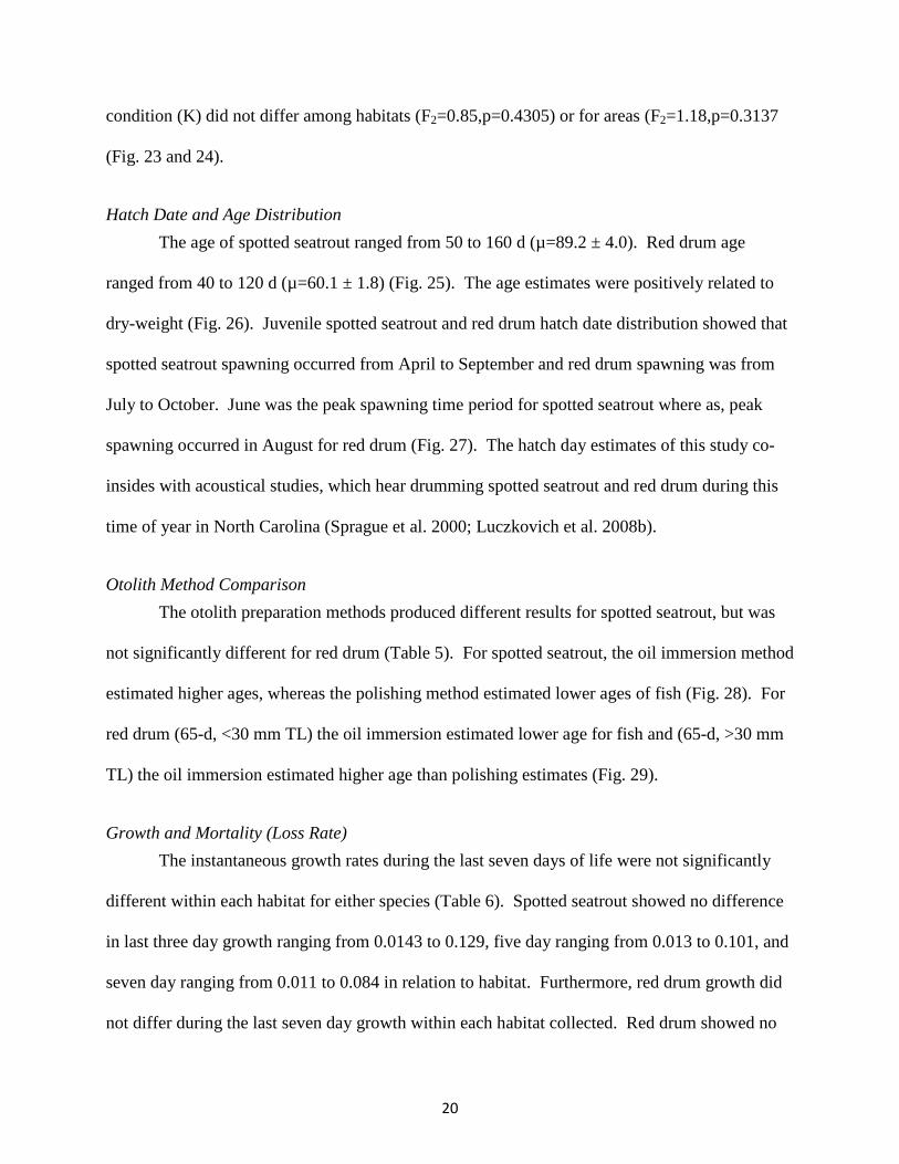
Hatch Date and Age Distribution

The age of spotted seatrout ranged from 50 to 160 d (µ=89.2 ± 4.0). Red drum age

ranged from 40 to 120 d (µ=60.1 ± 1.8) (Fig. 25). The age estimates were positively related to

dry-weight (Fig. 26). Juvenile spotted seatrout and red drum hatch date distribution showed that

spotted seatrout spawning occurred from April to September and red drum spawning was from

July to October. June was the peak spawning time period for spotted seatrout where as, peak

spawning occurred in August for red drum (Fig. 27). The hatch day estimates of this study co-

insides with acoustical studies, which hear drumming spotted seatrout and red drum during this

time of year in North Carolina (Sprague et al. 2000; Luczkovich et al. 2008b).

Otolith Method Comparison

The otolith preparation methods produced different results for spotted seatrout, but was

not significantly different for red drum (Table 5). For spotted seatrout, the oil immersion method

estimated higher ages, whereas the polishing method estimated lower ages of fish (Fig. 28). For

red drum (65-d, <30 mm TL) the oil immersion estimated lower age for fish and (65-d, >30 mm

TL) the oil immersion estimated higher age than polishing estimates (Fig. 29).

Growth and Mortality (Loss Rate)

The instantaneous growth rates during the last seven days of life were not significantly

different within each habitat for either species (Table 6). Spotted seatrout showed no difference

in last three day growth ranging from 0.0143 to 0.129, five day ranging from 0.013 to 0.101, and

seven day ranging from 0.011 to 0.084 in relation to habitat. Furthermore, red drum growth did

not differ during the last seven day growth within each habitat collected. Red drum showed no

21

significant differences within habitat in last three day growth ranging from 0.004 to 0.201, five

day ranging from 0.003 to 0.148, and seven day ranging from 0.003 to 0.171. Furthermore, there

was no difference in three, five, and seven day growth among the four groups defined by the

CLUSTER analysis (Table 7).

Daily spotted seatrout mortality rates from the field season (2009-2010) were 1.5%/d in

detritus, 1.7%/d in sand and 1.4%/d in SAV habitats. There was no significant difference (F2

=0.04, p=0.9646) in mortality rates among habitats. Daily mortality rates for red drum within

habitats in 2010 field season were in detritus (4.4%/d), in sand (2.3%/d), and SAV (4.9%/d);

there was no significant difference among habitats (F5=1.19,p=0.4131).


The one-way ANOSIM and non-metric multidimensional scaling (MDS) indicated that

the fish community did not differ in the presence of spotted seatrout or red drum or both species

present (Global R = -0.058, p=94.2%) (Fig. 30 and 31). The major of fish species contributing to

fish community among areas were bay anchovy (Anchoa mitchilli), inland silverside (Menidia

beryllina), and spot (Table 8).

Diet Composition

The cumulative prey curve showed a well defined asymptote for both species (Fig. 32),

indicating that the total sample size was adequate to describe the diets of red drum and spotted

seatrout using the 13 prey categories (Table 9). The percentages of empty stomachs varied

between the species. Stomachs that contained no food (n=81) for red drum and (n=45) for

spotted seatrout. The analysis identified 10 groups of prey consisting mostly of crustaceans for

both species. For red drum, amphipods, isopods, and mysids were the primary prey in the diet

and collectively occurred in 62.9% of the stomachs containing food (Table 10). These prey items

also accounted for >70.0% of the diet weight. Bivalves, insect nymphs, and gastropods

were absent from the red drum diet but present in the spotted sea trout diet. For spotted seatrout

mysids were the most dominant prey item occurring in 24.6% of the stomachs containing food

and accounting for >50% of the diet biomass (Fig. 33). Anchoa mitchilli, fish eggs and mysids

(IRI of 77%) occurred in 55% of spotted seatrout stomachs containing food. Polycheates were

present in 27.4% of the red drum stomachs containing food, but were absent in spotted seatrout

diet.

The results of the two way ANOSIM on diet composition showed that there were no

differences in diet among the sampling areas (R = 0.021, P < 0.27). However, there were

differences in diet between species (R = 0.274, P < 0.001). Most of the differences in diet

(SIMPER) were driven by mostly by isopods, mysids and amphipods (Fig. 34). Collectively

these three prey were responsible for 47.6% of the dissimilarity.

DISCUSSION

Habitat

Juvenile spotted seatrout abundance during sampling did differ by area (West, Central,

and East) and habitats along the river. The habitat effects on spotted seatrout occurred in SAV

where abundance was highest, but no differences existed for red drum in area or habitat. Studies

in other systems have shown that distribution patterns and abundances of spotted seatrout are

influenced by SAV densities in an aquatic system. For example, a study in western Florida

showed juvenile spotted seatrout and gray snapper (Lutjanus griseus) had a preference for basin

areas and SAV densities exceeding 1,000 shoots per square meters (Chester and Thayer 1990).

Additionally, spotted seatrout, red drum and other fishes are more associated with complex

vegetated areas than non-vegetated bottoms or marsh edges

23

(Stunz and Minello 2001; Nagelkerken and Van Der Velde 2002; Neahr et al. 2010). A predator

prey study on juvenile red drum demonstrated that complex habitats help lower mortality rates of

wild and reared red drum when pinfish (Lagodon rhomboids) and spotted seatrout predators were

present (Stunz and Minello 2001).

A resource map of SAV complex habitats along Pamlico River designated cover

classifications of SAV as dense (70-100%), patchy (5-70%) and absent (0-5%). The Pamlico

River is considered to have dense (66.8 ha) and patchy (21.0 ha) areas of SAV (NCDENR 2011).

Furthermore, proportionally the Pamlico River has 14.8% SAV and the majority of the river is

considered to be absent coverage (Joey Powers un-published data). This may explain why

juvenile red drum had higher abundance in detritus compared to SAV and sand. The difference

between spotted seatrout and red drum abundances among habitats may reflect that red drum are

more sensitive to density and size of complex habitats than spotted seatrout. The results from

this study suggest that habitat complexity has greater influence on juvenile red drum recruitment

than to spotted seatrout.

The purpose of this study was to analysis not only SAV habitats, but other substantial

habitats (detritus and sand) where spotted seatrout and red drum occur. Even though young-of-

year red drum prefer seagrass and are found in low abundance in areas without seagrass, they

may utilize other areas when seagrass is limited (Stunz et al. 2002a). Other studies suggest that

when SAV or seagrass meadows are less available, red drum will recruit to the next most

complex habitat (Series 1992; Baltz et al. 1993; Stunz et al. 2002a). A similar results was found

in this study, where the next most complex habitat studied was detritus. Juvenile red drum had

higher abundance in detritus compared to SAV.

24

Spotted seatrout individuals (27%) collected in the seine were >80 mm TL and 5% of

collected red drum individuals where >50 mm TL, which may imply individuals of a certain size

may have not been susceptible to the gear or movement between habitats was occurring. This

relates to other studies where >30 mm fish are rarely collected in the gear used (seine or benthic

sled) (McMichael and Peters 1989; Stunz et al. 2002a). Comparing detritus and/or organic matter

habitats to seagrass beds for recruitment of juvenile spotted seatrout and red drum are missing in

other studies. My study attempted to enlighten and investigate this issue by comparing two

habitats that are considered habitats (SAV and sand) to one not usually considered a habitat

(detritus).

The contingent theory may explain why the CPUE patterns of juvenile spotted seatrout

and red drum existed along the river. The Pamlico River empties into Pamlico Sound and most

salinities that were measured are not favorable for spawning ≤15.0 ppt (Saucier and Baltz 1993;

Rooker and Holt 1997). Spotted seatrout and red drum spawning could actually occur in

Pamlico Sound, with recruits migrating into the river (sink) while others stay out in the Sound

(source). Kraus and Secor (2004) showed that after spawning, white perch (Morone americana)

offspring recruited to freshwater, while others stayed in brackish habitats. They also concluded

that having these contingent individuals may help with maintaining population levels for

reproduction, which could be occurring with spotted seatrout and red drum in Pamlico River.

Environmental Data

Within the sampled areas (West, Central, and East) and habitats (detritus, sand, and SAV)

the environmental parameters did not differ except for pH and dissolved oxygen, which had high

values in Central and the most variability in the West. Salinity had high values in the East and

most variability in the West. Spotted seatrout occur in 18-32 ppt but are most abundant at 20 ppt

25

(McMichael and Peters 1989; Kupschus 2003; Wuenschel et al. 2004). In comparison, red drum

select areas of salinity of 0-34 ppt and moderately higher 35 ppt (Crocker et al. 1981; Peters and

McMichael 1987; Adams and Tremain 2000). In this study, salinities ranged from 0.4 to 21.4

ppt, with most spotted seatrout and red drum on average collected in salinities of 10.1 ppt and

12.5 ppt, respectively.

Another important environmental parameter essential for fish and aquatic life is dissolved

oxygen. Dissolved oxygen ranging from 4.2 to 8.8 mg/L is fundamentally important in

supporting juvenile spotted seatrout, with 6.5 mg/L being the optimal average for growth (Baltz

et al. 1998). Juvenile red drum are found in dissolved oxygen ranging from 3.7 to 10.2 mg/L

with 7.9 mg/L being the average ideal for growth (Baltz et al. 1998). In my study, dissolved

oxygen ranged from 2.15 mg/L to 12.12 mg/L, with higher abundance of juvenile spotted

seatrout caught at 7.9 mg/L. On the other hand, juvenile red drum were caught in higher

abundances at 9.1 mg/L. The dissolved oxygen ranges of my study covered the essential ranges

that spotted seatrout and red drum need for growth.

Age, Growth, and Mortality (Loss Rate)

Instantaneous growth rates (last 3, 5, and 7-d) were not significant among habitats for

both species, which may imply that they are not staying in a habitat long enough to make a

difference in growth. This may also indicate that the habitat effect is not strong enough to affect

habitat specific response. However, the highest overall growth rates were found in SAV for

spotted seatrout and detritus for red drum. The growth rates for both species observed in this

study are similar and followed the same patterns to others (Peters and McMichael 1987;

McMichael and Peters 1989; Stunz et al. 2002b).

26

Acquiring the most cost effective and precise techniques for calculating growth and age

estimates for fish species is essential in fisheries science. The technique of polishing otoliths has

been used in numerous studies for aging estimates (McMichael and Peters 1989; Prentice and

Dean 1991; Murphy and McMichael 2003) as well as the technique of embedding otoliths in oil

immersion for a period of time to clear (May and Jenkins 1992; Morales-Nin and Aldebert 1997;

Grorud-Colvert and Sponaugle 2006). However, validation between polishing and oil immersion

has not been determined in sciaenid species. My study suggests that the two methods (polish and

oil) show similar results between collected juvenile spotted seatrout and red drum.

Most spotted seatrout and red drum studies use the polishing method (David and Isely

1994; Baltz et al. 1998; Powell et al. 2000). My study showed that age estimates between both

methods for spotted seatrout were significant, with oil immersion having the best percent error

and estimating a higher age than polishing. This suggests that oil immersion should give a better

estimate of age for juvenile spotted seatrout 20-140 mm SL. The age estimates between both

methods for red drum were not significant and the percent error was almost equal between the

two. Because this is the case, both methods maybe adequate when aging 10-50 mm SL fish.

The use of oil immersion is easier because the otolith is submerged in oil immersion for four

weeks to clear, and then aging can proceed. The otolith submerged longer than four weeks have

less visible rings because the otolith starts to degrade (Secor 1991). Last and most important it

produces similar results to traditional embedding techniques (polishing) for red drum, which can

be difficult to age.

During the sampling period, daily loss rate was highest in sand habitats (1.7%/d)

compared to the more complex SAV and detritus. These results reinforce laboratory and field

study experiments, which show juvenile spotted seatrout and red drum are found in higher

27

abundances and preferring complex habitats than ones with less structural complexity (Stunz et

al. 2001; Neahr et al. 2010). In this study, movement to these more complex habitats may have

possibly helped reduce mortality of spotted seatrout. Our estimates of loss rate were slightly

higher than estimates from a study with similar size fish (16-144 mm) (Rutherford et al. 1989). A

different situation exists with red drum; higher daily mortality occurred in SAV habitats (4.9%/d)

compared to the other two habitats. One aspect may be that more SAV habitat existed toward

the mouth of the river. If red drum recruit into the river from the sound, the SAV may be the

first habitat where recruiting individuals occupy. In Tampa Bay Florida, Peters and McMichael

(1987) found that red drum size increased as collection progress upstream of the river. Similar

results were reported by Stunz and Minello (2001) studying captive and wild red drum, where

high mortality occurred in un-vegetated areas and medium levels in seagrass. Furthermore, it

may be a size-selective mortality because smaller red drum have a wider range of predators than

their larger counterparts spotted seatrout within these habitats (Sogard 1997).


In my study, the presence of spotted seatrout and red drum had no apparent effect on

community structure within the sampling area. Other studies have suggested that time of year

has an effect on community structure and the dominant species of that community. Species co-

occurrence can make species communities unique (Akin et al. 2003; Murphy and Secor 2006).

An example of this is a study by Series (1992), who found spotted seatrout and silver perch co-

occurring in the same marsh areas. However, this was not observed in the present study and

could be due to other influences. Rakocinski at el. (1992) found shifts in community structure

and dominating fish species during the spring, followed by changes in water temperature and

decrease in dissolved oxygen. In the present study, neither spotted seatrout nor red drum were

28

ever the dominant species collected and because of their low numbers they may not affect the

community.

Juvenile spotted seatrout and red drum distributions could be contributed to food

association or fish recruitment with wind direction. Hamner et al. (1988) found that plankitvorus

fish species were highly associated with the windward side of coral reefs waiting for

zooplankton (food) to float by. Elson (1939) analyzed how speckled trout (Salvelinus fontinalis)

moved in different water currents and found that fish placed in even current showed some

orientation and distribution as they swam against the current. Fish may recruit to an area along

the river because of wind driven inshore currents, which may have an effect on distribution of

young of year red drum (Stewart and Scharf 2008). In Elson’s study (1939) it was established

that in a low flow system, fish typically randomly wandered. My study could be during a period

of low water flow, with spotted seatrout and red drum randomly wandering to habitats. In my

study, juvenile spotted seatrout were larger (30-160 mm) and had higher abundance in SAV

habitats compared to juvenile red drum that were smaller (15-65 mm) and more abundant in

detritus habitats. My results suggest that more research is needed to fill the gap in how juvenile

spotted seatrout and red drum relate to detritus habitats compared to other habitats and how they

may benefit from it.

LITERATURE CITED

Adams, D. H., and D. M. Tremain. 2000. Association of large juvenile red drum, Sciaenops ocellatus, with an estuarine creek on the Atlantic coast of Florida. Environmental Biology of Fishes 58(2):183-194.

Adams, S. M. 1976. Feeding ecology of eelgrass fish communities. Transactions of the American Fisheries Society 105(4):514-519.

Akin, S., K. Winemiller, and F. Gelwick. 2003. Seasonal and spatial variations in fish and macrocrustacean assemblage structure in Mad Island Marsh estuary, Texas. Estuarine, Coastal and Shelf Science 57(1-2):269-282.

Amundsen, P. A., H. M. Gabler, and F. Staldvik. 1996. A new approach to graphical analysis of feeding strategy from stomach contents data modification of the Costello (1990) method. Journal of Fish Biology 48(4):607-614.

Ayvazian, S., L. Deegan, and J. Finn. 1992. Comparison of habitat use by estuarine fish assemblages in the Acadian and Virginian zoogeographic provinces. Estuaries and Coasts 15(3):368-383.

Bacheler, N. M., L. M. Paramore, J. A. Buckel, and J. E. Hightower. 2009. Abiotic and biotic factors influence the habitat use of an estuarine fish. Marine Ecology Progress Series 377:263-277.

Bacheler, N. M., L. M. Paramore, J. A. Buckel, and F. S. Scharf. 2008. Recruitment of juvenile red drum in North Carolina: spatiotemporal patterns of year-class strength and validation of a seine survey. North American Journal of Fisheries Management 28(4):1086-1098.

Bachman, P. M., and G. M. Rand. 2008. Effects of salinity on native estuarine fish species in South Florida. Ecotoxicology 17(7):591-597.

Baltz, D. M., J. W. Fleeger, C. F. Rakocinski, and J. N. McCall. 1998. Food, density, and microhabitat: factors affecting growth and recruitment potential of juvenile saltmarsh fishes. Environmental Biology of Fishes 53(1):89-103.

Baltz, D. M., C. Rakocinski, and J. W. Fleeger. 1993. Microhabitat use by marsh-edge fishes in a Louisiana estuary. Environmental Biology of Fishes 36(2):109-126.

30

Baltz, D. M., R. G. Thomas, and E. J. Chesney. 2003. Spotted seatrout habitat affinities in Louisiana. Pages 147-175 in Biology of the spotted seatrout. CRC Press.

Bloomfield, A., and B. Gillanders. 2005. Fish and invertebrate assemblages in seagrass, mangrove, saltmarsh, and nonvegetated habitats. Estuaries and Coasts 28(1):63-77.

Blott, S. J., and K. Pye. 2001. GRADISTAT: a grain size distribution and statistics package for the analysis of unconsolidated sediments. Earth Surface Processes and Landforms 26(11):1237-1248.

Boesch, D. 1977. A new look at the zonation of benthos along the estuarine gradient. Ecology of Marine Benthos 6:245-266.

Brown-Peterson, N. 2003. The reproductive biology of spotted seatrout. Pages 99–134 in The biology of spotted seatrout. CRC Press.

Brown-Peterson, N., P. Thomas, and C. Arnold. 1988. Reproductive biology of the spotted seatrout, (Cynoscion nebulosus), in south Texas. US National Marine Fisheries Service Fishery Bulletin 86(2):373-387.

Burgess, C. C., and A. J. Bianchi. 2004. An economic profile analysis of the commercial fishing industry of North Carolina including profiles for state-managed species. North Carolina Division of Marine Fisheries, Morehead City, NC.

Carr, W. E. S., and C. A. Adams. 1973. Food habits of juvenile marine fishes occupying seagrass beds in the estuarine zone near Crystal River, Florida. Transactions of the American Fisheries Society 102(3):511-540.

Chambers, P., E. Prepas, H. Hamilton, and M. Bothwell. 1991. Current velocity and its effect on aquatic macrophytes in flowing waters. Ecological Applications 1(3):249-257.

Chester, A. J., and G. W. Thayer. 1990. Distribution of spotted seatrout (Cynoscion Nebulosus) and gray snapper (Lutjanus Griseus) juveniles in seagrass habitats of western Florida Bay. Bulletin of Marine Science 46(2):345-357.

31

Clarke, K., and R. Gorley. 2006. PRIMER v6. User manual/tutorial. Plymouth routine in mulitvariate ecological research. Plymouth Marine Laboratory.

Clarke, K. R. 1993. Non-parametric multivariate analyses of changes in community structure. Australian journal of ecology 18(1):117-143.

Clarke, K. R., and R. M. Warwick. 2001. Changes in marine communities: an approach to statistical analysis and interpretation.

Collins, M., B. Callahan, B. Post, and A. Avildsen. 2003. Locating sciaenid spawning aggregations in anticipation of harbor modifications and reactions of spotted sea trout spawners to acoustic disturbance. Listening to fish: passive acoustic applications in marine fisheries:11-14.

Conservation, M. 1996. Magnuson-Stevens Fishery Conservation and Management Act. Public Law 94:265.

Copeland, B. 1966. Effects of decreased river flow on estuarine ecology. Journal (Water Pollution Control Federation) 38(11):1831-1839.

Copeland, B., R. G. Hodson, and S. R. Riggs. 1984. Ecology of the Pamlico River, North Carolina: an estuarine profile. North Carolina State University, Raleigh (USA). Dept. of Zoology; East Carolina University, Greenville, NC (USA). Dept. of Geology

Cortes, E. 1997. A critical review of methods of studying fish feeding based on analysis of stomach contents: application to elasmobranch fishes. Canadian Journal of Fisheries and Aquatic Sciences 54(3):726-738.

Cortes, E. 1998. Methods of studying fish feeding: Reply. Canadian Journal of Fisheries and Aquatic Sciences 55:2708.

Crocker, P. A., C. R. Arnold, J. D. Holt, and J. A. DeBoer. 1981. Preliminary evaluation of survival and growth of juvenile red drum (Sciaenops ocellata) in fresh and salt water. Journal of the World Mariculture Society 12(1):122-134.

32

Currin, B. M., J. P. Reed, and J. M. Miller. 1984. Growth, production, food consumption, and mortality of juvenile spot and croaker: a comparison of tidal and nontidal nursery areas. Estuaries and Coasts 7(4):451-459.

David, A., and J. Isely. 1994. Differences between the sagitta, lapillus, and asteriscus in estimating age and growth in juvenile red drum, (Sciaenops ocellatus). Fishery Bulletin 92(3):509-515.

de Morais, A. T., and L. T. De Morais. 1994. The abundance and diversity of larval and juvenile fish in a tropical estuary. Estuaries and Coasts 17(1):216-225.

Elson, P. F. 1939. Effects of current on the movement of speckled trout. Journal of the Fisheries Board of Canada 4(5):491-499.

Ferry, L., and G. Caillet. 1996. 1996. Sample size and data analysis: are we characterizing and comparing diet properly. Feeding Ecology and Nutrition in Fish:71-80.

Fitzgerald, J. M. 1998. Fish utilzation of submerged aquatic vegetation in the Pamlico River. MS thesis, East Carolina University, Greenville.

Fluharty, D. 2000. Habitat protection, ecological issues, and implementation of the Sustainable Fisheries Act. Ecological Applications 10(2):325-337.

Giese, G., H. B. Wilder, and G. G. Parker. 1985. Hydrology of major estuaries and sounds of North Carolina. Available from Dist Branch USGS 604 S. Pickett St., Alexandria, VA 22034. (USGS, Raleigh, NC), USGS Water-Supply Paper (2221):108.

Gray, C., R. Chick, and D. McElligott. 1998. Diel changes in assemblages of fishes associated with shallow seagrass and bare sand. Estuarine, Coastal and Shelf Science 46(6):849-859.

Grorud-Colvert, K., and S. Sponaugle. 2006. Influence of condition on behavior and survival potential of a newly settled coral reef fish, the bluehead wrasse (Thalassoma bifasciatum). Marine Ecology-Progress Series 327:279.

Guisan, A., S. B. Weiss, and A. D. Weiss. 1999. GLM versus CCA spatial modeling of plant species distribution. Plant Ecology 143(1):107-122.

Haines, E. 1977. The origins of detritus in Georgia salt marsh estuaries. Oikos:254-260.

33

Hamner, W., M. Jones, J. Carleton, I. Hauri, and D. M. B. Williams. 1988. Zooplankton, planktivorous fish, and water currents on a windward reef face: Great Barrier Reef, Australia. Bulletin of Marine Science 42(3):459-479.

Hansson, S. 1998. Methods of studying fish feeding: a comment. Canadian Journal of Fisheries and Aquatic Sciences 55(12):2706-2707.

Hare, J. A., and K. W. Able. 2007. Mechanistic links between climate and fisheries along the east coast of the United States: explaining population outbursts of Atlantic croaker (Micropogonias undulatus). Fisheries Oceanography 16(1):31-45.

Holt, G., and S. Holt. 2003. Effects of variable salinity on reproduction and early life stages of spotted seatrout. Pages 135-145

in Biology of the spotted seatrout. CRC Press.

Holt, S. A. 2008. Distribution of red drum spawning sites identified by a towed hydrophone array. Transactions of the American Fisheries Society 137(2):551-561.

Iversen, E. S., and D. C. Tabb. 1962. Subpopulations Based on Growth and Tagging Studies of Spotted Seatrout, Cynoscion nebulosus, in Florida. Copeia 1962(3):544-548.

Jensen, C. C. 2009. Stock Status of Spotted Seatrout, Cynoscion nebulosus, in North Carolina, 1991-2008.

Kraus, R. T., and D. H. Secor. 2004. Dynamics of white perch Morone americana population contingents in the Patuxent River estuary, Maryland, USA. Marine Ecology Progress Series 279:247-259.

Kupschus, S. 2003. Development and evaluation of statistical habitat suitability models: an example based on juvenile spotted seatrout Cynoscion nebulosus. Marine Ecology Progress Series 265:197-212.

Lankford, T., and T. Targett. 1994. Suitability of estuarine nursery zones for juvenile weakfish (Cynoscion regalis): effects of temperature and salinity on feeding, growth and survival. Marine Biology 119(4):611-620.

Levin, P., R. Petrik, and J. Malone. 1997. Interactive effects of habitat selection, food supply and predation on recruitment of an estuarine fish. Oecologia 112(1):55-63.

34

Levin, P. S., and G. W. Stunz. 2005. Habitat triage for exploited fishes: Can we identify essential. Estuarine, Coastal and Shelf Science 64(1):70-78.

Liebens, J. 2001. Heavy metal contamination of sediments in stormwater management systems: the effect of land use, particle size, and age. Environmental Geology 41(3):341-351.

Lin, J., H. Xu, C. Cudaback, and D. Wang. 2008. Inter-annual variability of hypoxic conditions in a shallow estuary. Journal of Marine Systems 73(1-2):169-184.

Loveland, P. J., and W. R. Whalley. 2000. Particle size analysis. Soil and Environmental analysis. 2nd Edition. KA Smith and CE Mullins (eds.). Marcel Dekker, New York:281-314.

Lucas, J. S., and P. C. Southgate. 2012. Aquaculture: Farming aquatic animals and plants. Wiley-Blackwell.

Luczkovich, J. J., D. A. Mann, and R. A. Rountree. 2008a. Passive acoustics as a tool in fisheries science. Transactions of the American Fisheries Society 137(2):533-541.

Luczkovich, J. J., R. C. Pullinger, S. E. Johnson, and M. W. Sprague. 2008b. Identifying sciaenid critical spawning habitats by the use of passive acoustics. Transactions of the American Fisheries Society 137(2):576-605.

Mabe, M. 2012. Biogeographic Characterization of Fishes from Intertidal Sandflats in Pamlico River, North Carolina. MS thesis, East Carolina University, Greenville.

MacRae, P. S. D. 2007. A community approach to identifying essential fish habitat of spotted seatrout, (Cynoscion nebulosus), in Barataria Bay, Louisiana. Louisiana State University and Agriciltural and Mechanical College.

MacRae, P. S. D., and J. J. H. Cowan. 2010. Habitat Preferences of Spotted Seatrout, (Cynoscion nebulosus), in Coastal Louisiana: A Step Towards Informing Spatial Management in Estuarine Ecosystems. Open Fish Science Journal 3:154-163.

Matlock, G. C. 1990. The life history of red drum. Pages 1-21 in Manual red drum aquaculture.

35

May, H. M. A., and G. P. Jenkins. 1992. Patterns of settlement and growth of juvenile flounder Rhombosolea tapirina determined from otolith microstructure. Marine ecology progress series. Oldendorf 79(3):203-214.

McConnaughey, R. A., and K. R. Smith. 2000. Associations between flatfish abundance and surficial sediments in the eastern Bering Sea. Canadian Journal of Fisheries and Aquatic Sciences 57(12):2410-2419.

McMichael, R. H., and K. M. Peters. 1989. Early life history of spotted seatrout, Cynoscion nebulosus (Pisces: Sciaenidae), in Tampa Bay, Florida. Estuaries and Coasts 12(2):98-110.

Montagna, P. A., M. Alber, P. Doering, and M. S. Connor. 2002. Freshwater inflow: science, policy, management. Estuaries and Coasts 25(6):1243-1245.

Moore, J. C., and coauthors. 2004. Detritus, trophic dynamics and biodiversity. Ecology Letters 7(7):584-600.

Moore, R. H. 1976. Observations on fishes killed by cold at Port Aransas, Texas, 11-12 January 1973. The Southwestern Naturalist:461-466.

Morales-Nin, B., and Y. Aldebert. 1997. Growth of juvenile (Merluccius merluccius) in the Gulf of Lions (NW Mediterranean) based on otolith microstructure and length-frequency analysis. Fisheries Research 30(1-2):77-85.

Murphy, M. D., and J. R. H. McMichael. 2003. Age Determination and Growth of Spotted Seatrout, (Cynoscion nebulosus) (Pisces: Sciaenidae). Pages 41 in Biology of the spotted seatrout.

Murphy, R. F., and D. H. Secor. 2006. Fish and blue crab assemblage structure in a US mid Atlantic coastal lagoon complex. Estuaries and Coasts 29(6):1121-1131.

Nagelkerken, I., Kleijnen, S.,Klop, T.,Van Den Brand, R.,de La Moriniere, E.C.,Van der Velde, G. 2001. Dependence of Caribbean reef fishes on mangroves and seagrass beds as nursery habitats: a comparison of fish faunas between bays with and without mangroves/seagrass beds. Marine Ecology Progress Series 214:225-235.

36

Nagelkerken, I., and G. Van Der Velde. 2002. Do non-estuarine mangroves harbour higher densities of juvenile fish than adjacent shallow-water and coral reef habitats in Curacao (Netherlands Antilles)? Marine Ecology Progress Series 245(Sutherland 1996):191-204.

NCDENR. 2011. Albemarle-Pamlico National Estuary Program (APNEP). North Carolina Submerged Aquatic Vegetation Map.

NCDMF. 2010a. North Carolina spotted seatrout fishery management plan - draft for public comment. North Carolina Division of Marine Fisheries, Morehead City, North Carolina.

NCDMF. 2010b. Red Drum and Spotted Seatrout. http://www.ncfisheries.net/stocks/reddrum.htm.

Neahr, T., G. Stunz, and T. Minello. 2010. Habitat use patterns of newly settled spotted seatrout in estuaries of the north-western Gulf of Mexico. Fisheries Management and Ecology 17(5):404-413.

Paperno, R., T. Targett, and P. Grecay. 2000. Spatial and temporal variation in recent growth, overall growth, and mortality of juvenile weakfish (Cynoscion regalis) in Delaware Bay. Estuaries and Coasts 23(1):10-20.

Peebles, E., and S. Tolley. 1988. Distribution, growth and mortality of larval spotted seatrout, Cynoscion nebulosus: a comparison between two adjacent estuarine areas of southwest Florida. Bulletin of Marine Science 42(3):397-410.

Perdue, B. E., D. R. Matthews, and D. Freeman. 2010. North Carolina Department of Environment and Natural Resources. Continental Shelf Research 7(11-12):1367-1381.

Peters, K. M., and R. H. McMichael. 1987. Early life history of the red drum, Sciaenops ocellatus (Pisces: Sciaenidae), in Tampa Bay, Florida. Estuaries and Coasts 10(2):92-107.

Peterson, G., and R. Turner. 1994. The value of salt marsh edge vs interior as a habitat for fish and decapod crustaceans in a Louisiana tidal marsh. Estuaries and Coasts 17(1):235-262.

Phelan, B., J. Manderson, A. Stoner, and A. Bejda. 2001. Size-related shifts in the habitat associations of young-of-the-year winter flounder (Pseudopleuronectes americanus): field observations and laboratory experiments with sediments and prey. Journal of Experimental Marine Biology and Ecology 257(2):297-315.

37

Pinkas, L. 1971. Food habits study. California Fish Game, Fish Bulletin, Sacramento,(152):5-10.

Powell, A. 2003. Larval abundance, distribution, and spawning habits of spotted seatrout (Cynoscion nebulosus) in Florida Bay, Everglades National Park, Florida. Fishery Bulletin-National Ocenic and Atmospheric Administration 101(3):704-711.

Powell, A. B., E. H. Laban, S. A. Holt, and G. J. Holt. 2000. Validation of age estimates from otoliths of larval and juvenile spotted seatrout, Cynoscion nebulosus. Fishery Bulletin 98(3):650-654.

Prentice, J. A., and J. W. J. Dean. 1991. Use of known-age red drums to validate scale and otolith ages and to estimate growth in fresh water. North American Journal of Fisheries Management 11(3):424-428.

Purtlebaugh, C. H., and M. S. Allen. 2010. Relative abundance, growth, and mortality of five age-0 estuarine fishes in relation to discharge of the Suwannee River, Florida. Transactions of the American Fisheries Society 139(4):1233-1246.

Rakocinski, C. F., Baltz, D.M., and Fleeger, J.W. 1992. Correspondence between environmental gradients and the community structure of marsh-edge fishes in a Louisiana estuary. Marine Ecology Progress Series 80:135-148.

Reynolds, J. B., B. Murphy, and D. Willis. 1996. Active Fish Capture Methods. Fisheries techniques, 2nd edition. American Fisheries Society, Bethesda, Maryland:193-220.

Ricker, W. E. 1975. Computation and interpretation of biological statistics of fish populations. Canada Fisheries and Marine Service 191:383.

Riggs, B. J. C. a. S. R. 1984. The Ecology of the Pamlico River, North Carolina: an Estuarine Profile. NC Fish and Wildlife Service:1-69.

Rogers, S. 1992. Environmental factors affecting the distribution of sole (Solea solea) within a nursery area. Netherlands Journal of Sea Research 29(1-3):153-161.

Rooker, J. R., and S. A. Holt. 1997. Utilization of subtropical seagrass meadows by newly settled red drum Sciaenops ocellatus: patterns of distribution and growth. Marine Ecology Progress Series 158:139-149.

38

Rooker, J. R., S. A. Holt, M. A. Soto, and G. Joan Holt. 1998. Postsettlement patterns of habitat use by sciaenid fishes in subtropical seagrass meadows. Estuaries and Coasts 21(2):318-327.

Rozas, L. P., and W. E. Odum. 1988. Occupation of submerged aquatic vegetation by fishes: testing the roles of food and refuge. Oecologia 77(1):101-106.

Rutherford, E. S., T. W. Schmidt, and J. T. Tilmant. 1989. Early life history of spotted seatrout (Cynoscion nebulosus) and gray snapper (Lutjanus griseus) in Florida Bay, Everglades National Park, Florida. Bulletin of Marine Science 44(1):49-64.

Saucier, M. H., and D. M. Baltz. 1993. Spawning site selection by spotted seatrout, Cynoscion nebulosus, and black drum, Pogonias cromis, in Louisiana. Environmental Biology of Fishes 36(3):257-272.

Scharf, F. S. 2000. Patterns in abundance, growth, and mortality of juvenile red drum across estuaries on the Texas coast with implications for recruitment and stock enhancement. Transactions of the American Fisheries Society 129(6):1207-1222.

Scharf, F. S., Manderson, J.P.,Fabrizio, M.C., J. P. Pessutti, J. E. Rosendale, R. J. Chant, and A. J. Bejda. 2004. Seasonal and interannual patterns of distribution and diet of bluefish within a Middle Atlantic Bight estuary in relation to abiotic and biotic factors. Estuaries and Coasts 27(3):426-436.

Schramm, H. L., Armstrong, M.L.,Funicelli, N.A.,Green, D.M., D. P. Lee, R. E. Manns, B. D. Taubert, and S. J. Waters. 1991. The status of competitive sport fishing in North America. Fisheries 16(3):4-12.

Secor, D. H., Dean, J.M.,Laban, E.H.,Electric Power Research Institute,Belle W. Baruch Institute for Marine Biology,Coastal Research, editor. 1991. Manual for otolith removal and preparation for microstructural examination, volume 1.

Series, M. E. P. 1992. Correspondence between environmental gradients and the community structure of marsh-edge fishes in a Louisiana estuary. Marine Ecology Progress Series 80:135-148.

Smith, N., C. Jones, and J. Van Montfrans. 2008. Spatial and temporal variability of juvenile spotted seatrout Cynoscion nebulosus growth in Chesapeake Bay. Journal of Fish Biology 73(3):597-607.

39

Smith, T. I. J., W. E. Jenkins, M. R. Denson, and M. R. Collins. 2001. Stock enhancement research with anadromous and marine fishes in South Carolina. Ecology of Aquaculture Species and Enhancement of Stocks:175.

Sogard, S. M. 1997. Size-selective mortality in the juvenile stage of teleost fishes: a review. Bulletin of Marine Science 60(3):1129-1157.

Sprague, M. W., Luczkovich, J.J.,Pullinger, RC,Johnson, SE, T. Jenkins, and H. Daniel III. 2000. Using spectral analysis to identify drumming sounds of some North Carolina fishes in the family Sciaenidae. Journal of the Elisha Mitchell Scientific Society 116(2):124-145.

Stewart, C. B., and F. S. Scharf. 2008. Estuarine recruitment, growth, and first-year survival of juvenile red drum in North Carolina. Transactions of the American Fisheries Society 137(4):1089-1103.

Stunz, G. W., P. S. Levin, and T. J. Minello. 2001. Selection of estuarine nursery habitats by wild-caught and hatchery-reared juvenile red drum in laboratory mesocosms. Environmental Biology of Fishes 61(3):305-313.

Stunz, G. W., and T. J. Minello. 2001. Habitat-related predation on juvenile wild-caught and hatchery-reared red drum Sciaenops ocellatus (Linnaeus). Journal of Experimental Marine Biology and Ecology 260(1):13-25.

Stunz, G. W., T. J. Minello, and P. S. Levin. 2002a. A comparison of early juvenile red drum densities among various habitat types in Galveston Bay, Texas. Estuaries and Coasts 25(1):76-85.

Stunz, G. W., T. J. Minello, and P. S. Levin. 2002b. Growth of newly settled red drum Sciaenops ocellatus in different estuarine habitat types. Marine Ecology Progress Series 238:227-236.

Subrahmanyam, C., and C. Coultas. 1980. Studies on the animal communities in two north Florida salt marshes Part III. Seasonal fluctuations of fish and macroinvertebrates. Bulletin of Marine Science 30(4):790-818.

Takade, H., and L. Paramore. 2007. Stock status of the northern red drum stock. North Carolina Division of Marine Fisheries, Morehead City, NC.

40

Ter Braak, C. 1994. Canonical community ordination. Part I: Basic theory and linear methods. Ecosience 1(2):127-140.

Thayer, G. W., A. B. Powell, and D. E. Hoss. 1999. Composition of larval, juvenile, and small adult fishes relative to changes in environmental conditions in Florida Bay. Estuaries and Coasts 22(2):518-533.

Tolan, J. M., S. A. Holt, and C. P. Onuf. 1997. Distribution and community structure of ichthyoplankton in Laguna Madre seagrass meadows: potential impact of seagrass species change. Estuaries and Coasts 20(2):450-464.

Tsuzuki, M. Y., R. O. Cavalli, and A. Bianchini. 2003. Effect of salinity on survival, growth, and oxygen consumption of the pink-shrimp Farfantepenaeus paulensis (Perez-Farfante 1967). Journal of Shellfish Research 22(2):555-560.

Weinstein, M., S. Weiss, and M. Walters. 1980. Multiple determinants of community structure in shallow marsh habitats, Cape Fear River Estuary, North Carolina, USA. Marine Biology 58(3):227-243.

Wilson, J. A., L. Vigliola, and M. G. Meekan. 2009. The back-calculation of size and growth from otoliths: validation and comparison of models at an individual level. Journal of Experimental Marine Biology and Ecology 368(1):9-21.

Wuenschel, M., R. Werner, and D. Hoss. 2004. Effect of body size, temperature, and salinity on the routine metabolism of larval and juvenile spotted seatrout. Journal of Fish Biology 64(4):1088-1102.

Wurts, W. A. 1998. Why can some fish live in fresh water, some in salt water, and some in both. World Aquaculture 29(1):65.

Xu, H., J. Lin, and D. Wang. 2008. Numerical study on salinity stratification in the Pamlico River Estuary. Estuarine, Coastal and Shelf Science 80(1):74-84.

41

1

Table 1: Average monthly water quality estimates (±SD) for habitats studying along the Pamlico River, North Carolina from August 2

through November (2009-2010). 3

Month Area Wind (m/s) Water temp (°C) D.O. (mg/L) pH Salinity (ppt)

August Detritus 1.5(1.4) 30.3(0.6)

Sand 1.8(1.6) 30.3(0.9)

SAV 2.4(2.7) 30.5(1.1)

September Detritus 1.6(2.5) 26.2(2.0)

Sand 2.4(2.2) 26.5(1.1)

SAV 1.3(1.6) 26.6(1.3)

October Detritus 2.7(1.8) 19.5(3.0)

Sand 2.3(2.7) 19.2(2.6)

SAV 1.5(1.4) 18.6(2.4)

November Detritus 1.5(1.7) 15.4(1.5)

Sand 1.5(1.4) 15.4(1.5)

SAV 0.9(0.9) 15.3(1.6)

7.5(3.2)

7.8(1.0)

7.9(1.1)

7.1(1.4)

7.7(1.4)

7.9(1.3)

8.5(1.9)

8.3(1.5)

8.2(1.6)

8.8(1.2)

8.9(1.3)

8.9(1.5)

8.4(0.5)

8.4(0.2)

8.4(0.3)

8.1(0.2)

8.5(0.2)

8.3(0.2)

7.7(0.4)

8.1(0.4)

8.0(0.4)

8.2(0.2)

8.3(0.1)

8.2(0.2)

8.8(3.0)

8.1(3.2)

7.1(2.0)

11.2(2.9)

10.3(3.6)

9.1(2.6)

10.7(4.3)

11.5(4.8)

10.8(5.6)

13.4(3.4)

12.1(4.7)

12.7(4.3)

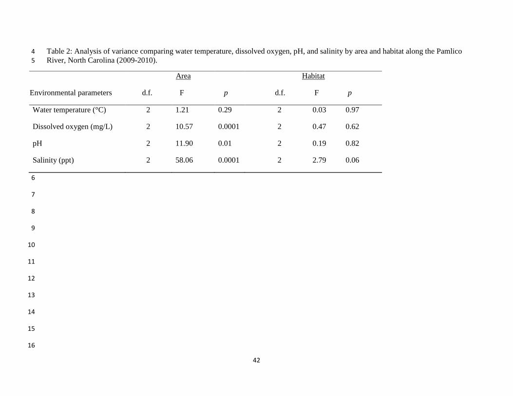
42

Table 2: Analysis of variance comparing water temperature, dissolved oxygen, pH, and salinity by area and habitat along the Pamlico 4

River, North Carolina (2009-2010). 5

Environmental parameters

d.f.

Area

F

p

Habitat

d.f. F p

Water temperature (°C)

Dissolved oxygen (mg/L)

pH

Salinity (ppt)

2

2

2

2

1.21

10.57

11.90

58.06

0.29

0.0001

0.01

0.0001

2 0.03 0.97

2 0.47 0.62

2 0.19 0.82

2 2.79 0.06

6

7

8

9

10

11

12

13

14

15

16

43

17

Table 3: The four groups (G) of CLUSTER analysis representing mean percent sediment type for 18

each grouping in Pamlico River, North Carolina. 19

Sediment G1 G2 G3 G4 Biological material Silt Very fine sand Fine sand Medium-fine sand Medium sand Course sand Gravel

22.0 15.6

28.3 18.7 9.2 5.5 1.2 0.02

.19 9.4 21.3

32.8 24.4

7.7 2.8

8.7

0.30 2.9 3.6 5.0 26.6 44.3 16.8 2.4

.52 1.5 4.2 79.5 50.7 20.4 6.1 1.5

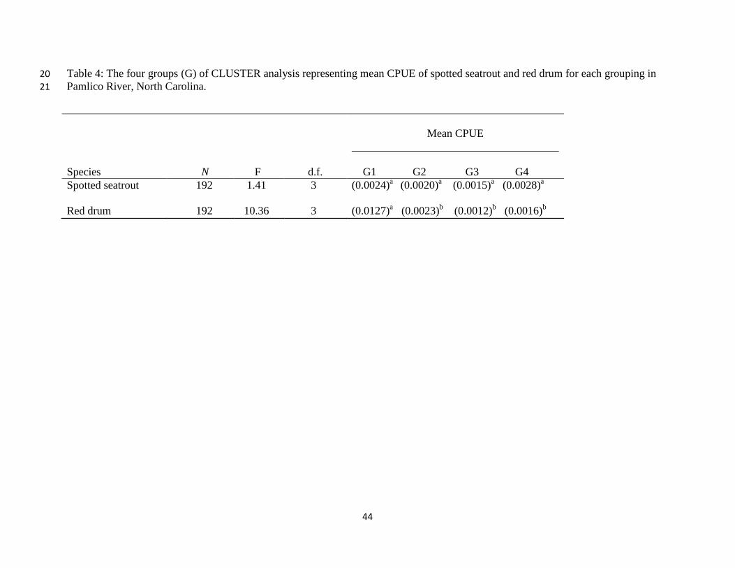
44

Table 4: The four groups (G) of CLUSTER analysis representing mean CPUE of spotted seatrout and red drum for each grouping in 20

Pamlico River, North Carolina. 21

Species

N

F

d.f.

Mean CPUE

G1 G2 G3 G4 Spotted seatrout Red drum

192

192

1.41

10.36

3

3

(0.0024)a (0.0020)a (0.0015)a (0.0028)a (0.0127)a (0.0023)b (0.0012)b (0.0016)b

45

Table 5: Analysis comparing the ages of oil immersion and polishing methods of juvenile spotted seatrout (30 to 160 mm TL) and red 22

drum (15 to 65 mm TL). Where CV= coefficient of variation; D= percent error; r2= the number of replicate interpretation square; t= t-23

value; d.f. =degrees; p=probability. 24

25

Method Regression Percent error

D=CV/√R r2 t d.f. p

Spotted seatrout

Oil

Polishing

Red drum

Oil

Polishing

y=0.9858x+40.353

y=1.0101x+30.36

y=1.7734x+14.729

y=1.2015x+31.539

5.53

7.85

6.57

6.33

0.79

-2.43 44 0.0195

0.75

0.76

0.29 82 0.7748

0.51

46

26

Table 3: Back-calculation of the last 3, 5, and 7 days of growth and average instantaneous 27

growth rate per day (±SD) of juvenile spotted seatrout and red drum in relation to habitat type. 28

Growth d.f. F p Instantaneous growth rate per day

Spotted seatrout

3 day growth

5 day growth

7 day growth

Red drum

3 day growth

5 day growth

7 day growth

2

2

2

2

2

2

0.04

0.06

0.06

2.71

2.83

2.80

0.9601

0.9415

0.9407

0.0735

0.0655

0.0676

0.036(0.024)

0.033(0.021)

0.032(0.019)

0.023(0.033)

0.020(0.026)

0.018(0.024)

29

30

31

32

33

34

35

36

37

38

39

40

41

47

Table 4: Back-calculation of the last 3, 5, and 7 days of growth of juvenile spotted seatrout and 42

red drum using the groupings from the CLUSTER analysis. 43

Growth d.f. F p

Spotted seatrout

3 day growth

5 day growth

7 day growth

Red drum

3 day growth

5 day growth

7 day growth

3

3

3

3

3

3

0.65

0.65

0.73

2.10

1.93

1.75

(0.58)a

(0.58)a

(0.54)a

(0.10)a

(0.13)a

(0.16)a

44

45

46

47

48

49

50

51

52

53

54

55

56

57

48

Table 5: The average per seine haul CPUE of the three most important species in each section in 58

Pamlico River, NC. Fish were collected twice a month using a beach bag seine from August to 59

November 2009-2010 (Mabe 2012). 60

Species Section Per seine haul abundance

M. beryllina West 11.75

A. mitchilli 12.17

L. xanthurus 2.41

A. mitchilli Central 18.4

M. beryllina 8.52

L. xanthurus 3.34

A. mitchilli East 17.82

M. beryllina 4.76

L. xanthurus 1.69

61

62

63

64

65

66

67

68

49

Table 6: Names, categories, and aggregated prey categories used in the diet analysis.

Category Description

Amphipoda

Fish

Calanoida

Caridea

Cladocera

Gastropods

Insects

Isopoda

Mysidae

Annelids

Shrimp like in form

All fishes, remains and eggs (exclusively Anchoa mitchilli)

Calanoid copepods

Shrimp

Small crustaceans

Snails

All larval and adult insects (almost exclusively dipteran larvae)

Small crustaceans

All mysid shrimps

Polychaeta

50

Table 7: Diet composition of red drum and spotted sea trout in Pamlico River estuary. The diet indices are defined in the text (%FO, percentage frequency of; %N, percentage numerical abundance; %W, percentage Biomass; and % IRI, index of relative importance on a percent basis (%IRI). The unknown/other category includes unidentified items, sand, and plant material.

Red drum Spotted seatrout

Category %FO %(W) %N %IRI %FO %(W) %N %IRI

Amphipoda

A. mitchilli

Bivalvia

Calanoida

Caridea

Cladocera

Diptera

Egg

Gastropoda

Insect nymph

Isopoda

Mysidae

Polychaeta

Unknown/Other

14.5

6.5

0.0

4.8

1.6

3.2

1.6

4.8

0.0

0.0

21.0

27.4

12.9

1.6

22.1

6.5

0.0

1.8

3.4

0.6

3.4

2.5

0.0

0.0

27.7

21.5

9.6

0.8

12.4

2.4

0.0

2.9

0.6

12.9

0.6

2.4

0.0

0.0

24.7

35.3

5.3

0.6

14.2 8.7 4.7 4.2 2.2

1.6 15.9 12.0 6.7 8.4

0.0 1.4 1.4 0.4 0.1

0.7 5.8 2.3 4.6 1.1

0.2 5.8 9.1 2.1 1.8

1.2 5.8 1.1 2.1 0.5

0.2 4.3 1.6 3.5 0.6

0.7 14.5 3.6 12.3 6.4

0.0 1.4 0.3 0.7 0.0

0.0 2.9 7.2 0.7 0.6

31.3 5.8 4.1 1.4 0.9

44.4 24.6 51.8 60.0 77.1

5.5 0.0 0.0 0.0 0.0

0.1 2.9 0.8 1.4 0.2

69

70

71

72

51

73

Figure 1: The 65 km study site of the Pamlico River from the Fork Point Island to the mouth of 74

the Pungo River, North Carolina and the three sections West, Central and East and all 36 sub-75

sites. Red marks represented potential sites not selected by the random number generator, and 76

pink circles (six stations within each section) represent sites that were included in the study. 77

78

52

79

Figure 2. Two-dimensional diagram representing prey frequency of occurrence and abundance of 80

a fish taxon (Amundsen et al. 1996). 81

82

53

West Central East

Dis

solv

ed o

xyge

n (m

g/L)

0

2

4

6

8

10

12

14a b

a

83

Figure 3. Mean dissolved oxygen (mg/L) from Fork Point Island, NC to the mouth of the Pungo 84

River, NC sampled twice a month from August to November (2009-2010) using an 18-m long 85

bag seine in Pamlico River, North Carolina. The dots represent outliers and the whiskers 86

represent the minimum and maximum of 100% of the values. 87

54

West Central East

pH

6.5

7.0

7.5

8.0

8.5

9.0

9.5

a

b

b,c

88

Figure 4. Mean water quality parameter pH from Fork Point Island, NC to the mouth of the 89

Pungo River, NC sampled twice a month from August to November (2009-2010) using an 18-m 90

long bag seine in Pamlico River, North Carolina. The dots represent outliers and the whiskers 91


93

94

55

West Central East

Sal

inity

(pp

t)

0

5

10

15

20

25

ab

c

95

Figure 5. Mean salinity (ppt) water quality parameter from Fork Point Island, NC to the mouth 96

of the Pungo River, NC sampled twice a month from August to November (2009-2010) using an 97

18-m long bag seine in Pamlico River, North Carolina. The dots represent outliers and the 98

whiskers represent the minimum and maximum of 100% of the values. 99

100

101

56

West Central East

Win

d sp

eed

(m/s

)

0

2

4

6

8

10 a

a,b

a,c

102

Figure 6. Mean wind speed (m/s) water quality parameter from Fork Point Island, NC to the 103

mouth of the Pungo River, NC sampled twice a month from August to November (2009-2010) 104

using an 18-m long bag seine in Pamlico River, North Carolina. The dots represent outliers and 105

the whiskers represent the minimum and maximum of 100% of the values. 106

107

108

109

110

111

112

113

114

115

116

57

Detritus Sand SAV0

2

4

6

8

10

12

14a

a a

Dis

solv

ed o

xyge

n (m

g/L)

117

Figure 7. Mean dissolved oxygen (mg/L) of habitat from Fork Point Island, NC to the mouth of 118

the Pungo River, NC sampled twice a month from August to November (2009-2010) using as 119



122

123

124

125

126

127

128

129

58

Detritus Sand SAV6.5

7.0

7.5

8.0

8.5

9.0

9.5a

a a

pH

130

Figure 8. Water quality parameter pH of habitat from Fork Point Island, NC to the mouth of the 131

Pungo River, NC sampled twice a month from August to November (2009-2010) using an 18-m 132

long bag seine in Pamlico River, North Carolina. The dots represent outliers and the whiskers 133


135

136

137

138

139

140

141

142

143

144

59

Detritus Sand SAV

0

5

10

15

20

25a a a

Sal

inity

(pp

t)

145

Figure 9. Mean salinity (ppt) water quality parameter of habitat from Fork Point Island, NC to 146

the mouth of the Pungo River, NC sampled twice a month from August to November (2009-147

2010) using an 18-m long bag seine in Pamlico River, North Carolina. The dots represent 148

outliers and the whiskers represent the minimum and maximum of 100% of the values. 149

150

151

152

153

154

155

156

157

158

159

60

Detritus Sand SAV

0

2

4

6

8

10

a

a a

Win

d sp

eed

(m/s

)

160

Figure 10. Mean wind speed (m/s) water quality parameter of habitat from Fork Point Island, 161

NC to the mouth of the Pungo River, NC sampled twice a month from August to November 162

(2009-2010) using an 18-m long bag seine in Pamlico River, North Carolina. The dots represent 163

the minimum and maximum of 100% of the values. 164

165

166

167

168

169

170

171

172

173

174

61

175

West Central East

Pe

rce

nt s

edim

ent

(%)

0

20

40

60

80

100Biological material Gravel Course sand Medium sand Medium-fine sand Fine sand Very fine sand Silt

176

Figure 11. Percent sediment composition along a downstream gradient per area along Pamlico 177

River, North Carolina from Fork Point Island, NC to the mouth of the Pungo River, NC sampled 178

twice a month from August to November (2009-2010). 179

62

SandMud

Gravel

80%

30%

5%

Trace

1:11:9 9:1

Gravel %

Gravel

Muddy Gravel Muddy Sandy Gravel

Gravelly Mud Gravelly Muddy Sand

Slightly Gravelly

Mud

Slightly GravellySandy Mud

Slightly GravellyMuddy Sand

Mud Sandy Mud Muddy SandSand

Slightly Gravelly

Sand

Gravelly Sand

Sandy Gravel

64

TEXTURAL GROUP:

SEDIMENT NAME:

Slightly Gravelly Sand

Slightly Fine Gravelly Medium Sand

SAMPLE IDENTITY:

WestCentralEast

180

Figure 12. Sediment pyramid of sites sampled along Pamlico River, North Carolina in relation 181

to practical size from Fork Point Island, NC to the mouth of the Pungo River, NC sampled twice 182

a month from August to November (2009-2010). 183

184

63

45 37 60 33 57 49 39 50 35 36 31 53 54 41 64 52 55 62

S ite s

1 0 0

8 0

6 0

4 0

Sim

ilarit

yR e se m b la n c e : S 1 7 B ray C u r t is s im ila r ity

a re aC e n tra lE a s tW e st

Group 1 Group 2 Group 4Group 3

185

Figure 13. CLUSTER analysis of sediment type composition sampled along Pamlico River, 186

North Carolina from Fork Point Island, NC to the mouth of the Pungo River, NC. With four 187

groups represented and site 45 (Group 1) located in the Central area having low levels of 188

similarity (<58%) when compared to all other sites (>50%). 189

190

64

West Central East

Per

cent

site

sam

pled

hab

itat

(%)

0

20

40

60

80

100DetritusSandSAV

191

Figure 14. Percent of sampling sites classified as (detritus, sand, and SAV) in Pamlico River 192

from Fork Point Island, NC to the mouth of the Pungo River, NC sampled twice a month from 193

August to November (2009-2010) and using an 18-m long bag seine in Pamlico River, North 194

Carolina. 195

65

West Central East0

20

40

60

80

100DetritusSandSAV

Per

cent

hab

itat (

%)

35%41%

24%

3%

15%

82%

75%25%

0%

(75%)

(11%)(14%)

(0%)

(33%)

(67%)

(24%)(31%)

(45%)

196

Figure 15. Percent of sampling sites classified as (detritus, sand, SAV) and percent spotted 197

seatrout and red drum ( ) caught in each habitat along Pamlico River from Fork Point Isalnd, NC 198

to the mouth of the Pungo River, NC sampled twice a month from August to November (2009-199

2010) and using an 18-m long bag seine. 200

201

202

203

204

205

66

Total length (mm)

0 10 20 30 40 50 60 70 80 90 100 110 120 130 140 150 160

Fre

que

ncy

0

2

4

6

8

10

12

14

16

18

20

Spotted seatrout (N=56)Red drum (N=86)

206

Figure 16. Length frequency distribution of juvenile spotted seatrout and red drum from August 207

through November (2009-2010) along Pamlico River, North Carolina. Juvenile spotted seatrout 208

lengths caught from 2009-2010 ranged from 30 mm to 160 mm with a mean (66.5± 4.4 mm). 209

Juvenile red drum lengths ranged from 15 to 65mm with a mean (32.6 ± 1.1 mm). 210

211

67

Mea

n C

PU

E (

num

ber/

255m2 )

0.000

0.005

0.010

0.015

0.020

0.025

0.030

a

a,b

b

Spotted seatrout

(N=191,F=3.97,df=2,P=0.02)

West Central East0.000

0.005

0.010

0.015

0.020

0.025

0.030

a

a

a

Red drum

(N=191,F=2.25,P=0.10)

212

Figure 17. Mean catch per unit effort (CPUE) of juvenile spotted (black) seatrout and red drum 213

(gray) per area (±1SE). Fishes were collected and all areas where sampled each time along 214

sandy beach habitats from Fork Point Island, NC to the mouth of the Pungo River, NC twice a 215

month from August to November (2009-2010) using an 18-m long bag seine in Pamlico River, 216

North Carolina. 217

68

Mea

n C

PU

E (

num

ber/

255

m2 )

0.00

0.01

0.02

0.03

0.04

0.05

a

b

a,c

Spotted seatrout (N=191,F=3.97,df=2,P=0.02)


0.01

0.02

0.03

0.04

0.05a

a

a

Red drum(N=191,F=3.08,df=2,P=0.05)

218

219

Figure 18. Mean catch per unit effort (CPUE) of juvenile spotted seatrout (black) and red drum 220

(gray) per habitat type (±1SE). Fishes were collected and all areas where sampled each time 221

along sandy beach habitats from Fork Point Island, NC to the mouth of the Pungo River, NC 222

twice a month from August to November (2009-2010) using an 18-m long bag seine in Pamlico 223

River, North Carolina. 224

225

69

Detritus Sand SAV

Mea

n C

PU

E (

num

ber/

m2 )

0.00

0.01

0.02

0.03

0.04

0.05

52%

19%20% 24%

28%

57%

226

Figure 19. Catch per unit effort (CPUE) of juvenile spotted seatrout (black) and red drum 227

(white) per habitat type (±1SE). Fishes were collected and all areas where sampled each time 228




232

70

Mea

n C

PU

E (

num

ber/

m2 )

0.000

0.005

0.010

0.015

0.020


0.005

0.010

0.015

0.020

DetritusSandSAV

*

*

Spotted seatrout

Red drum

233

Figure 20. Mean catch per unit effort (CPUE) of juvenile spotted seatrout (top) and red drum 234

(bottom) per habitat type (±1SE). Fishes were collected and all areas where sampled each time 235




71

To

tal l

engt

h (m

m)

0

20

40

60

80

100

*

West Central East0

20

40

60

80

100

**

Spotted seatrout

Red drum

239

Figure 21. Total length (mm) of juvenile spotted seatrout (top) and red drum (bottom) among 240

area (±1SE). Larger juvenile spotted seatrout and red drum occurring in the West area. Fishes 241

were collected and all areas where sampled each time along sandy beach habitats from Fork 242

Point Island, NC to the mouth of the Pungo River, NC twice a month from August to November 243

(2009-2010) using an 18-m long bag seine in Pamlico River, North Carolina. 244

72

20 40 60 80 100 120 140

Dry

wei

ght

(mg)

0

2

4

6

8

10

y=2E-06x3.1606

r2=0.9938

Standard length (mm)

20 40 60 80 100 120 140

0.0

0.2

0.4

0.6

0.8

y=6E-08x3.8407

r2=0.9027

Spotted seatrout

Red drum

245

Figure 22. Juvenile spotted seatrout (black) and red drum (white) dry-weight (g) to length 246

relationship. Standard length (mm) plotted on dry-weight (g) with power regression line overlaid. 247

Fishes were collected and all areas where sampled each time along sandy beach habitats from 248

Fork Point Island, NC to the mouth of the Pungo River, NC twice a month from August to 249

November (2009-2010) using an 18-m long bag seine in Pamlico River, North Carolina. 250

251

73

Con

diti

on fa

cto

r (K

)

0.14

0.16

0.18

0.20

0.22

0.24

0.26

0.28

0.30

0.32

0.34

0.36


0.05

0.10

0.15

0.20

0.25

0.30

0.35

0.40

a

a a

a

a a

Spotted seatrout

Red drum

252

Figure 23. Fulton’s Condition Factor (FCF) of juvenile spotted seatrout in (detritus, sand, and 253

SAV) relation to habitat along Pamlico River, North Carolina (±1SE). Fishes were collected and 254

all areas where sampled each time along sandy beach habitats from Fork Point Island, NC to the 255

mouth of the Pungo River, NC twice a month from August to November (2009-2010) using an 256



259

74

Con

ditio

n fa

ctor

(K

)

0.14

0.16

0.18

0.20

0.22

0.24

0.26

0.28

0.30

0.32

0.34

0.36


0.05

0.10

0.15

0.20

0.25

0.30

0.35

0.40

Spotted seatrout

Red drum

aa

a

aa a

260

Figure 24. Fulton’s Condition Factor (FCF) of juvenile spotted seatrout (black) and red drum 261

(white) in (detritus, sand, and SAV) relation to area along Pamlico River, North Carolina (±1SE). 262



November (2009-2010) using an 18-m long bag seine in Pamlico River, North Carolina. The dots 265

represent outliers and the whiskers represent the minimum and maximum of 100% of the values. 266

267

75

Age (days)

40 60 80 100 120 140 160

Fre

quency

0

5

10

15

20

Age (days)

20 40 60 80 100 120 140 1600

5

10

15

20

Spotted seatrout

Red drum

268

Figure 25. Age frequency of juvenile spotted seatrout (black) and red drum (white) along 269

Pamlico River, North Carolina. Juvenile spotted seatrout lengths caught from 2009-2010 ranged 270

from 40 to 120-d with a mean (89.2± 4.0). Juvenile red drum lengths ranged from 50 160-d with 271

a mean (60.1 ± 1.8). Fishes were collected and all areas where sampled each time along sandy 272

beach habitats from Fork Point Island, NC to the mouth of the Pungo River, NC twice a month 273

from August to November (2009-2010) using an 18-m long bag seine in Pamlico River, North 274

Carolina. 275

76

40 60 80 100 120 140 160

Dry

-wei

ght

(mg)

0

1

2

3

4

5

6

7y=0.0320e0.0311t

r2=0.4995

Age (days)

40 60 80 100 120 140 160

0.0

0.1

0.2

0.3

0.4

0.5

0.6

y=0.0040e0.0409t

r2=0.7836

Red drum

Spotted seatrout

276

Figure 26. Juvenile spotted seatrout (black) and red drum (white) dry-weight (g) to age (days) 277

relationship. Age (days) plotted on dry-weight (g) with exponential regression line overlaid. 278




282

77

Hatch date (day of year)

100 120 140 160 180 200 220 240 260 280 300 320

Fre

quen

cy

0

5

10

15

20

25

30

35April May June July Aug Sep Oct

283

Figure 27. Hatch date of juvenile spotted seatrout (black) and red drum (white) per day of year, 284

from August to November (2009-2010) using an 18-m long bag seine in Pamlico River, North 285

Carolina. Fishes were collected and all areas where sampled each time along sandy beach 286

habitats from Fork Point Island, NC to the mouth of the Pungo River, NC. Juvenile spotted 287

seatrout and red drum peak hatching occurring in June and August, respectively. 288

289

290

78


0 20 40 60 80 100 120 140 160 180

Oto

lith

age

(day

s)

20

40

60

80

100

120

140

160

180

200

220

OilPolishLinear (oil)Linear (polish)

291

Figure 28. Juvenile spotted seatrout age to length relationship compare oil immersion and 292

polishing techniques for ageing. Standard length (mm) plotted on age (days) with linear 293

regression line overlaid. Oil immersion gives a higher estimate of age than the embedding 294

method. Fishes were collected and all areas where sampled each time along sandy beach habitats 295

from Fork Point Island, NC to the mouth of the Pungo River, NC twice a month from August to 296


298

79


0 10 20 30 40 50 60 70

Oto

lith

age

(day

s)

0

20

40

60

80

100

120

140

OilPolishLinear (oil)Linear (polish)

299

Figure 29. Juvenile red drum age to length relationship compare oil immersion and polishing 300

techniques for ageing. Standard length (mm) plotted on age (days) with linear regression line 301

overlaid. The oil immersion gives a lower estimate for fish <30 mm TL. However, the 302

embedding method gives a higher estimate for fish >30 mm TL. Fishes were collected and all 303

areas where sampled each time along sandy beach habitats from Fork Point Island, NC to the 304

mouth of the Pungo River, NC twice a month from August to November (2009-2010) using an 305

18-m long bag seine in Pamlico River, North Carolina. 306

307

308

309

310

311

312

313

80

-0 .1 2 -0 .1 0 -0 .0 8 -0 .0 6 -0 .0 4 -0 .0 2 0 0 .0 2 0 .0 4 0 .0 6 0 .0 8 0 .1 0 0 .1 2 0 .1 4 0 .1 6R

0

2 0 2F

requ

ency

314

Figure 30. ANOSIM comparisons between the presences or absence of juvenile spotted seatrout 315

and red drum along Pamlico River, North Carolina from Fork Point Island, NC to the mouth of 316

the Pungo River, NC sampled twice a month from August to November (2009-2010) and using 317

an 18-m long bag seine in Pamlico River, North Carolina. The one-way ANOSIM indicated that 318

the presence or absence of both species had no affect on fish community structure (Global R=-319

0.058, p=94.2%). 320

81

T r an s f o r m : P r es en c e/ab s en c eR es em b lan c e : S 1 7 Br ay C u r t is s im ila r ity

S p ec iesS P S TS P S T & R DR DN e ith e r

2 D S tr es s : 0 .2 1

321

Figure 31. The non-metric multidimensional scaling (MDS) plot showing the presence or 322

absence of juvenile spotted seatrout and red drum in relation to community structure along 323

Pamlico River, North Carolina from Fork Point Island, NC to the mouth of the Pungo River, NC 324

sampled twice a month from August to November (2009-2010) and using an 18-m long bag 325

seine in Pamlico River, North Carolina. 326

327

328

329

330

331

332

82

2 4 6 8 10 12 14 16 18 20

Nuu

mbe

r of

new

pre

y ca

tego

ries

2

4

6

8

10

12

Number of stomach examined

1 2 3 4 5 6 7 8 9 10 11 12 13 14 15 16 17 18 19

Nuu

mbe

r of

new

pre

y ca

tego

ries

2

4

6

8

10

12

14 Spotted Seatrout

Red Drum

333

Figure 32. Cumulative prey curve for the total number of juvenile red drum and spotted seatrout. 334

The black line is the mean number of new prey items calculated for each sample size after a 100-335

times randomization order of stomach contents. 336

83

Red drum

0

10

20

30

40

50

60

Amphipoda

A. mitchilli

Calanoida

Caridea

Cladocera

Egg

Gastropoda

Insect nymph

Isopoda Mysidae

Polychaeta

Unkown

Spotted seatrout

FO(%)

0 5 10 15 20 25 30

Pi(%

)

0

10

20

30

40

50

60

70

Amphipoda

A. mitchilliBivalvia

Calanoida

Caridea

Cladocera

Egg

Gastropoda

Insect nymph

Isopoda

Mysidae

Polychaeta

Unkown

337

Figure 33. Relationship among prey specific abundance (%Pi) and frequency of occurrence 338

(%FO) of food categories in juvenile red drum and spotted seatrout diet. Plots based on 339

modified Costello graphical method (Amundsen et al. 1996). 340

341

84

342

Figure 34. (a) Patterns in diet composition (%number) for juvenile red drum and spotted seatrout 343

collected during August through November 2009-2010 in Pamlcio River, North Carolina 344

demonstrated in a multidimensional scaling (NMDS) plot. Symbols that are close together have 345

greater similarity than symbols that are further apart, bubble plots (b-d) are superimposed from 346

the NMDS diet analysis. (a) Triangles represent spotted seatrout and closed circles represent red 347

drum. Bubble size approximates relative proportion of a given taxa in the diet: (b) isopods, (c) 348

mysids (d) amphipods. 349

350

351

352

353

354

355

356

85

APPENDIX A: ANIMAL USE PROTOCOL APPROVAL 357

358

359

distribution patterns of juvenile spotted seatrout ( july, 2012

Documents