distributed - hipore.comhipore.com/stcc/2016/ijcc-vol4-no3-2016-pp1-13-guo.pdf · services...

Services Transactions of Cloud Computing (ISSN 2326-7550) Vol. 4, No. 3, July-September 2016

DISTRIBUTED ALGORITHMS FOR SPATIAL RETRIEVAL QUERIES IN

GEOSPATIAL ANALYSIS Qiulei Guo1, Balaji Palanisamy1, Hassan A. Karimi1 and Liming Zhang2

School of Information Sciences, University of Pittsburgh1

School of Architecture, Carnegie Mellon University2

[email protected], [email protected], [email protected], [email protected]

Abstract The proliferation of data acquisition devices like 3D laser scanners had led to the burst of large-scale spatial terrain data which imposes many challenges to spatial data analysis and computation. With the advent of several emerging cloud technologies, a natural and cost-effective approach to managing such large-scale data is to store and process such datasets in a publicly hosted cloud service using modern distributed computing paradigms such as MapReduce. For several key spatial data analysis and computation problems, polygon retrieval is a fundamental operation which is often computed under real- time constraints. However, existing sequential algorithms fail to meet this demand effectively given that terrain data in recent years have witnessed an unprecedented growth in both volume and rate. In this work, we present a MapReduce-based parallel polygon retrieval algorithm which aims at minimizing the IO and CPU loads of the map and reduce tasks during spatial data processing. Our proposed algorithm first hierarchically indexes the spatial terrain data using a quad-tree index, with the help of which, a significant amount of data is filtered out in the pre- processing stage based on the query object. In addition, a prefix tree based on the quad-tree index is built to query the relationship between the terrain data and query area in real time which leads to significant savings in both I/O load and CPU time. The performance of the proposed techniques is evaluated in a Hadoop cluster and the results demonstrate that the proposed techniques are flexible and scalable. Our quad tree indexing with prefix tree acceleration lead to more than 35% reduction in execution time of the polygon retrieval operation over existing distributed algorithms while the quad tree indexing without prefix tree works best for the proximity query. Keywords: [MapReduce, Polygon Retrieval, Proximity Query, Quad-Tree Indexing, Prefix Tree]

__________________________________________________________________________________________________________________

1. INTRODUCTION The proliferation of cost-effective data acquisition devices

like 3D laser scanners has enabled the acquisition of massive

amounts of terrain data at an ever-growing volume and rate.

With the advent of several emerging collaborative cloud

technologies, a natural and cost-effective approach to managing

such large-scale data is to store and share such datasets in a

publicly hosted cloud service and process the data within the

cloud itself using modern distributed computing paradigms

such as MapReduce. Examples of applications that process such

terrain data include urban environment visualization, shadow

analysis, visibility computation, and flood simulation. Many

geo-spatial queries on such large datasets are intrinsically

complex to solve and are often computed under real-time

constraints, thus requiring fast response times for the queries.

However, most existing sequential algorithms fail to meet this

demand effectively given that terrain data in the recent years

have witnessed an unprecedented growth in both volume and

rate. Therefore, a common approach to speed up spatial query

processing is parallelizing the individual operations on a cluster

of commodity servers.

In GIS applications, there are several common spatial query

algorithms such as polygon retrieval and proximity query.

Polygon retrieval is a fundamental geospatial operation which

is often computed under real-time constraints. Polygon retrieval

involves retrieval of all terrain data within a given polygon’s

boundary of interest for further analysis (Mark de Berg, 2008;

Willard, 1982). As for proximity query, it retrieves all spatial

entities within a distance from a target location. We note that

terrain data is usually represented using one of the common data

structures to approximate surface, for example, digital elevation

model (DEM) and triangulated irregular network(TIN). Among

these existing structures, TIN (Peucker, Fowler, Little, & Mark,

1978) is a widely used model and it consists of irregularly

distributed nodes and lines arranged in a network of non-

overlapping triangles. Compared to other spatial data structures,

TIN requires considerably higher storage as it can be used to

represent surfaces with much higher resolution and detail. For

instance, a TIN dataset for the state of Pennsylvania would

require up to 60TB. Therefore, real-time processing of such a

large amount of data is not possible through sequential

computations and a distributed parallel computation is needed to

meet the fast response time requirements.

We argue that such large scale spatial datasets can effectively

leverage the MapReduce programming model (Dean &

Ghemawat, 2008) to compute spatial operations in parallel. In

doing so, key challenges include how to organize, partition and

distribute a large scale spatial dataset across 10s of 100s of nodes

in a cloud data center so that applications can query and analyze

the data quickly and cost-effectively. Furthermore, polygon

retrieval is a CPU-intensive operation whose performance

heavily depends on the computation load causing performance

1 doi: 10.29268/stcc.2016.4.3.1


4

bottlenecks when dealing with very large datasets. Therefore, a

suitable algorithm needs to minimize the computation load on

the individual map and reduce tasks as well. In this paper, we

develop a MapReduce-based parallel algorithm for distributed

processing of polygon retrieval operation in Hadoop

("Hadoop,"). Our proposed algorithm first hierarchically

indexes the spatial terrain data using a quad-tree index, with the

help of which, a significant amount of data is filtered out in the

pre-processing stage based on the query object. In addition, a

prefix tree based on the quad-tree index is built to query the

relationship between the terrain data and query area in real time

which leads to significant savings in both I/O load and CPU

time. We evaluate the performance of the proposed algorithm

through experiments on our Hadoop cluster consisting of 6

servers. Our experiment results show that the proposed

algorithm is flexible, scalable and performs faster than existing

distributed algorithms.

The rest of the paper is organized as follows: Section 2

reviews the related work and in Section 3, we provide a

background on TIN and overview the polygon retrieval

problem. Section 4 describes our proposed MapReduce based

algorithms and the optimization techniques. We discuss the

experiment results in Section 5 and conclude in Section 6.

2. RELATED WORKPolygon retrieval is a common operation for a diverse

number of spatial queries in many GIS applications.

( W i l l a r d , 1 9 8 2 ) proposed the polygon retrieval

problem formally and devised an algorithm that runs in

𝑂(𝑁𝑙𝑜𝑔64) time in the worst-case. To speed up this query

further, several efficient sequential algorithms have been

proposed. The most notable among these include the

algorithms presented in (Mark de Berg, 2008; Paterson & Frances

Yao, 1986; Sioutas, Sofotassios, Tsichlas, Sotiropoulos, & Vlamos,

2008; Tung & King, 2000). However, with the recent massive

growth in terrain data, these sequential algorithms fail to meet

the demands of real- time processing.

As cloud computing has emerged to be a cost-effective

and promising solution for both compute and data intensive

problems, a natural approach to ensure real-time processing

guarantees is to process such spatial queries in parallel

effectively leveraging modern cloud computing technologies. In

this context, some earlier work (Karimi, Roongpiboonsopit, &

Wang, 2011) had explored the feasibility of using Google App

Engine, the cloud computing technology by Google, to

process TIN data. Since MapReduce/Hadoop has become the

defacto standard for distributed computation on a massive

scale, some recent works have developed several

MapReduce-based algorithms for GIS problems. The authors

in ( P u r i , A g a r w a l , H e , & P r a s a d , 2 0 1 3 ) propose

and implement a MapReduce algorithm for distributed

polygon overlay computation in Hadoop. The authors in (Ji et

al., 2012) present a MapReduce-based approach that construct

inverted grid index and processes kNN query over large

spatial data sets. The technique presented in (Akdogan,

Demiryurek, Banaei-Kashani, & Shahabi, 2010) creates a

unique spatial index and Voronoi diagram for given points in

2D space and enables efficient processing of a wide range of

geospatial queries such as RNN, MaxRNN and kNN with the

MapReduce programming model. Hadoop-GIS (Wang et al.,

2011) and Spatial-Hadoop (Eldawy, Li, Mokbel, & Janardan,

2013; Eldawy & Mokbel, 2013) are two scalable and high-

performance spatial data processing system for running large-

scale spatial queries in Hadoop. These systems provide support

for some fundamental spatial queries including the minimal

bounding box query. However, they do not directly support

polygon retrieval operation addressed in our work. In our work,

we primarily focus on the polygon retrieval queries on spatial

data and we devise specific optimization techniques for an

efficient implementation of the parallel polygon retrieval

operation in MapReduce.

3. BACKGROUNDIn this section, we provide the required background and

preliminaries about the TIN spatial data storage format and a

brief overview of MapReduce based parallel processing of

large-scale datasets.

A. TIN Data

TIN (Peucker et al., 1978) is a commonly used model for

representing spatial data and it consists of irregularly distributed

nodes and lines arranged in a network of non-overlapping

triangles. TIN data typically gets generated from raster data such

as LIDAR (Light Detection and Ranging) which is a remote

sensing method that uses light in the form of a pulsed laser to

measure ranges to the Earth surface. These light pulses

combined with other data recorded by the airborne system

generate precise, three-dimensional information about the

shape and surface characteristics. In our work, we consider

TIN data generated from LIDAR data using the Delaunay

triangulation algorithm implemented by the LASTool

(LAStools). An example of LIDAR data and its

corresponding TIN representation is shown in Figure 1(a) and

Figure 1(b) respectively.

When it comes to data representation, TINs are traditionally

stored as a file, in ASCII or the ESRI TIN dataset file format.

To improve the efficiency of processing large TIN datasets,

(Al-Salami, 2009; Hanjianga, Limina, & Longa) have proposed

new TIN data structures and operations for spatial databases

that allow storing, querying and reconstructing TINs more

efficiently. However, we note that there are no standards on the

data structures and operations for TIN (Karimi et al., 2011);

Oracle has defined a proprietary data type and operations for

managing large TINs in their own spatial database (Kothuri,

Godfrind, & Beinat, 2007). In our work, we adopt the data

format from (Karimi et al., 2011) which comprises of two

types of data entities: TIN Points and TIN Triangles, as

shown in Figure 2. Both types have their unique IDs. The

TIN Points type has five properties and the TIN Triangles

entity has three properties. For the TIN Point, the

Adj_ TriangleID[] array stores the IDs of its adjacent

triangles. For the TIN Triangle, the Point ID array and

Coordinate array contain the IDs and coordinates for the three

vertices of each triangle.

B. Polygon Retrieval

In this subsection, we describe the polygon retrieval problem

using data represented in TIN. Given the boundary of a

simple polygon, the polygon retrieval operation retrieves all

the terrain data, represented by TIN that intersects with the

polygon. As there could be many possible situations of

2


intersection (Clementini, Sharma, & Egenhofer, 1994), here for

the sake of simplicity, we consider an intersection when at

least one of its vertex of the TIN triangles intersects with

the query area. We note that point-in-polygon algorithms can

be used to determine whether a point is inside or outside the

polygon. One such well-known algorithm is ray tracing

algorithm which is usually referred to as crossing number

algorithm or even-odd rule algorithm (Al-Salami, 2009) in the

literature. An example of the polygon retrieval is given in Figure

3.

(a) LIDAR Point cloud (b) TIN surface

Fig. 1: LIDAR and TIN surface

Fig. 2: TIN representation

Fig. 3 Polygon Retrieval

C. Proximity Query

Besides the polygon retrieval, there is also another

common spatial query in GIS application, which is

proximity query. It retrieves all spatial entities within a

distance from a target location. In our case, a proximity

query retrieves all the terrain data, represented by TIN that

are within the given distance from the target location. Since

the basic unit of TIN is a triangle, here for the sake of

simplicity, we consider the triangle is within the distance

from the given target location if the distance between the

target location and any one of the triangle’s vertexes is

smaller than the given radius. An example of the proximity

query is given in Figure 4.

Fig. 4 Proximity Query

B. MapReduce overview

In this work, we are focused on MapReduce-based

parallel processing of TIN for the spatial query operation.

We note that in addition to the programming model,

MapReduce ( D e a n & G h e m a w a t , 2 0 0 8 ) also

includes the system support for processing the

MapReduce jobs in parallel in a large scale cluster. Apache

Hadoop ("Hadoop,") is a popular open source

implementation of the MapReduce framework. Hadoop is

composed of two major parts: storage model, Hadoop

Distributed File System (HDFS) and compute model

(MapReduce). A key feature of the MapReduce

3


framework is that it can distribute a large job into

several independent map and reduce tasks over several

nodes of a large data center and process them in parallel.

MapReduce can effectively leverage data locality and

processing on or near the storage nodes and result in faster

execution of the jobs. The framework consists of one

master node and a set of slave nodes. In the map phase,

the master node schedules and distributes the individual

map tasks to the worker nodes. A map task executing in

a worker node processes the smaller chunk of the file

stored in HDFS and passes the intermediate results to the

appropriate reduce tasks executing in a set of worker nodes.

The reduce tasks collect the intermediate results from the

map tasks and combine/reduce them to form the final

output. Since each map operation is independent of the

others, all maps can be performed in parallel. It is also

the same with reducers as each reducer works on a

mutually exclusive set of intermediate results produced by

mappers.

4. MAPREDUCE-BASED SPATIAL QUERYIn this section, we first present a naive implementation of

parallel spatial retrieval operation using MapReduce and

illustrate its performance. We then present our proposed

optimization techniques that significantly improves this

basic spatial retrieval algorithm.

A. Basic MapReduce Algorithm for Spatial Query

An intuitive and straight-forward MapReduce-based

spatial retrieval implementation is to process all the terrain

data stored in HDFS as part of the MapReduce job. Each

mapper will process an input split and check whether a

given point is within the boundary of the query area or

not. The HDFS partitions the TIN data into several chunks

(64 MB blocks by default) and each map task would

process one chunk of data in parallel. Unfortunately this

basic MapReduce algorithm (Algorithm1) has several key

performance limitations. Firstly, for each query the

algorithm reads all terrain data from the HDFS and

processes them in the map phase. This approach is not

efficient in situations when the query area is a smaller

portion of the whole dataset, where the system does not

need to scan all terrain data to obtain accurate results. We

also note that the point in polygon computation in the

map phase is a reasonably CPU consuming operation and

hence performing this computation for a huge amount of

data will result in significantly longer job execution times.

Our proposed algorithm employs a sequence of

optimization techniques that overcome the above-

mentioned shortcomings. First, our proposed technique

divides the whole dataset stored in HDFS into several

chunks of files based on a quad- tree prefix. Then for

each range query, we use a prefix tree to organize the set

of quad-indices whose corresponding grids intersect the

query area. Prior to processing a query, we employ these

indices to filter the unnecessary TIN data as part of the

data filtering stage so that unwanted data processing is

minimized in the map phase. Finally, the proposed

approach pre-tests the relationship between the TIN data

and the query shape through the built prefix tree in the

map function in order to minimize the computation. We

describe the essence and details of these techniques in

the following subsections.

Algorithm 1 Basic MapReduce Spatial Query

1: point id: a point ID

2: T IN point: a TIN point in space

3: procedure MAP(point id, TIN point)

4: get the boundary of the query area from the global

share memory of Hadoop

5: if tin point is within the boundary

6 : then

7： emit the key-value pair (point id, TIN point)

8： else

7: return

8: end if

9: end procedure

B. Indexing Terrain Data

To accelerate the processing of terrain data, we divide

the entire space based on a quad-tree (Pajarola, Antonijuan,

& Lario, 2002) and index each TIN record using the quad-

tree. Quad-tree is a common tree data structure used in

many geospatial applications which partitions a two-

dimensional space by recursively subdividing the space into

four equal regions. Compared with other spatial indices such

as R-tree or uniform grid index, the quad-tree has several

advantages for polygon retrieval. For instance, unlike the

index of R-tree which needs to be built by the insertion of

the terrain data one after another while maintaining the

tree’s balance structure which takes O(n ∗ logn) time, quad-

tree index does not need to maintain a real tree and can be

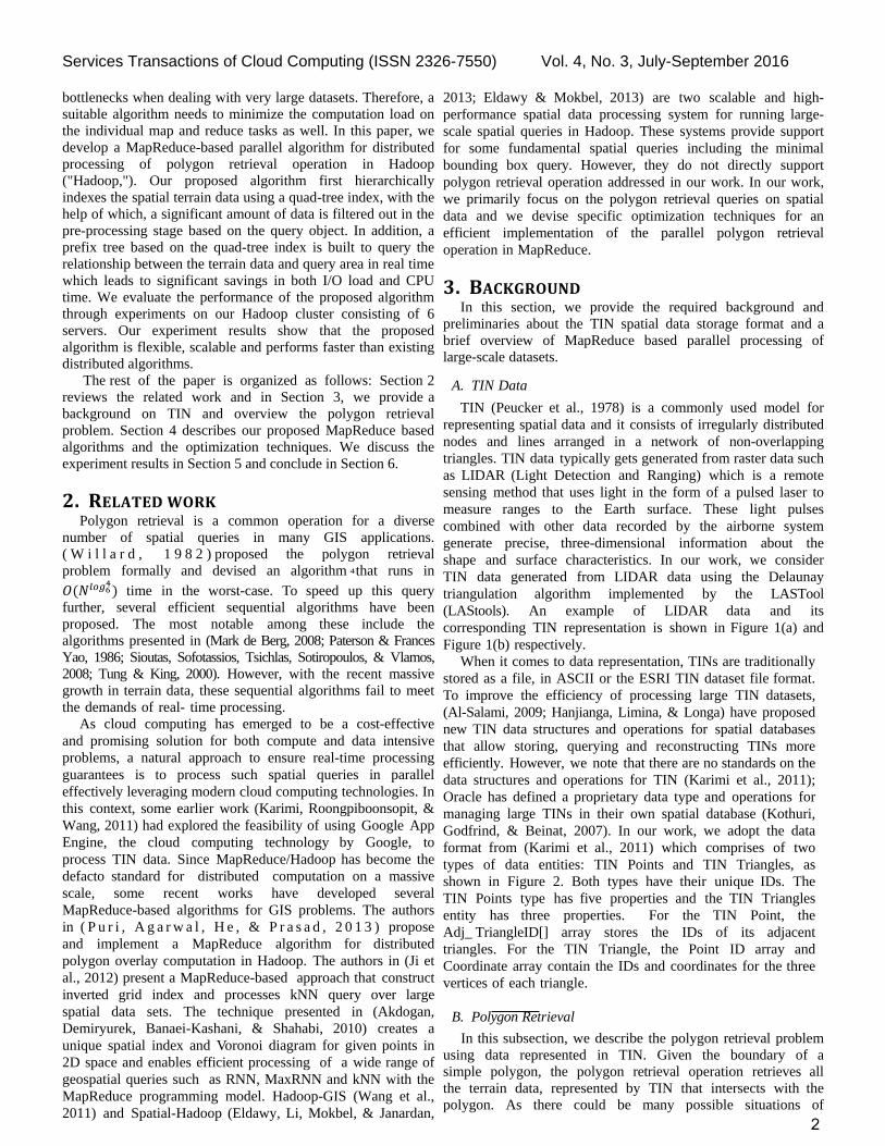
used to partition the space directly as shown in Fig 5(b). In

addition, with the quad-tree index, we can even infer the

topological relationship of the terrain data and the query

area from the indices’ prefix directly.

To decide whether the prefix of a quad-tree exists in a

given set of index entries, it would cost O(k ∗n) time for a

straight- forward algorithm, where k is the length of the

quad-tree index (also the depth of the quad-tree) and n is the

number of entries the indices set. Thus, when n and k

get larger, the cost of the algorithm will grow

significantly. In the next subsection, we propose a prefix

tree structure organizing grid entries that interact with the

query area with the cost of only O(k) time.

4


(a) Built Quad-Tree (b) Quad-index partitioning

(c) Polygon Query on Quad-Indexing (d) Proximity Query on Quad-Indexing

Fig. 5: Quad Tree-Indexing

For uniformly distributed point sets, good expected case

performance can be achieved by simple decompositions of

space into a regular grid of hyper cubes. The regular grids

have many good properties. For example, if n points are

chosen independently from a uniform distribution on the

unit square, then proximity query finds the nearest neighbor

of a query point in constant expected time(Bentley, Weide,

& Yao, 1980).

For the R-Tree, we generally adopt the R-Tree indexing

on Hadoop from (Cary, Sun, Hristidis, & Rishe, 2009). The

core idea is to run MapReduce jobs to sample the spatial

data from the given dataset. Then build the R-Tree from the

sample data and do the partition.

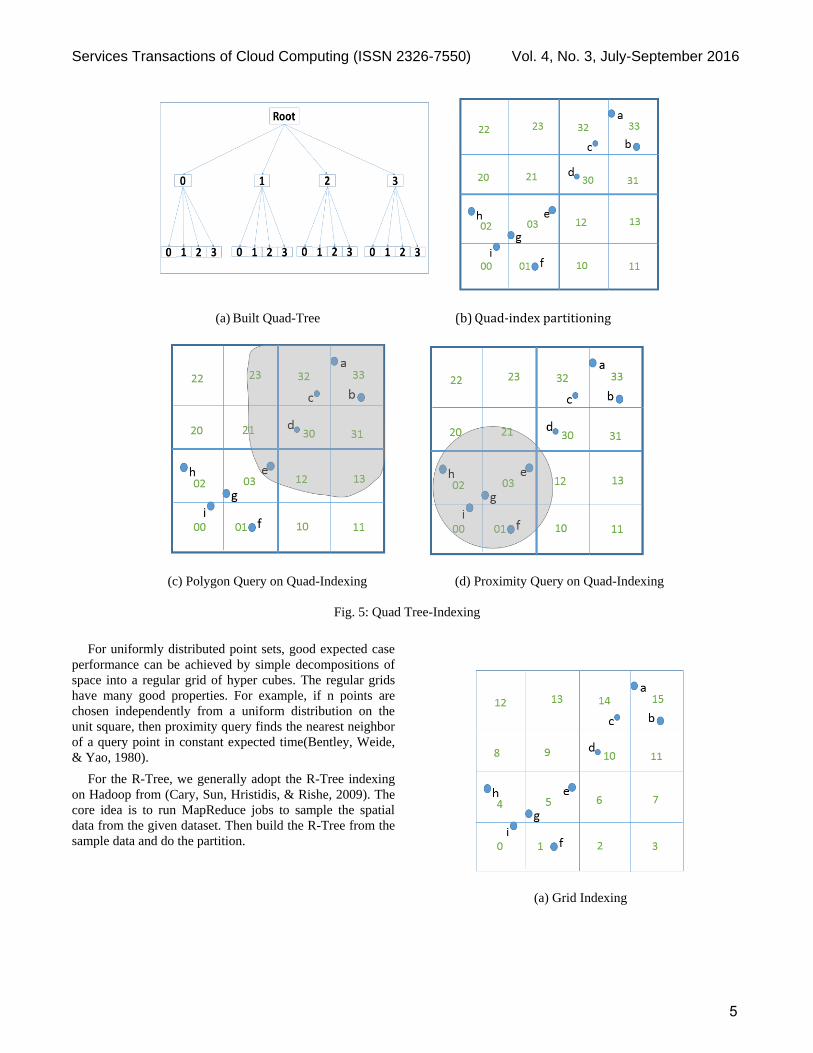
(a) Grid Indexing

5


(b) Polygon Query on Grid Index (c) Proximity Query on Grid Index

Figure 6: Grid Indexing

(a) Built R-tree (b) R-tree partitioning

(c) Polygon Query on R-tree partitioning (d) Proximity Query on R-tree partitioning

Fig. 7: R-tree Indexing

The examples that compares quad-tree indexing, grid-

indexing, and R-tree indexing are illustrated in Figures

5, 6 and 7. Figure 5(b) shows the partitioning of the

whole space based on the quad-tree index of length 2

directly. In Figure 6(a), we partition the space into 4*4

regular grids. In Figure 7(a), we build a R-tree

representation of the same space by going over the

elements in the terrain and inserting them to the tree for

6


the spatial partition shown in Figure 7(b). Next, we show

how the quad-tree index helps infer the topological

relationships using the example shown in Figure 5(c). In

the figure, we find the query area shown as a gray region

and the set of grid indices that intersect with this gray

query area are {30, 31, 32, 33, 23, 21, 12, 13, 03}. A

key observation here is that if a grid cell is within a

query area, then all its sub grids are also guaranteed to

be within the query area. Therefore the grids’ set {30, 31,

32, 33} can be combined into a single grid cell {3} and

the interacted indices set in Figure 5(c) can be abbreviated

to {3, 23, 21, 12, 13, 03}. Thus, if the prefix of a spatial

object’s quad-index exists in a set, then the object is

guaranteed to be within the query area. This property of

the proposed indexing scheme avoids the point-in-polygon

computation in the map phase enabling the MapReduce

jobs to complete significantly faster.

C. Organizing the index using Prefix Tree

A prefix tree, also called radix tree or trie, is an ordered

tree data structure that is used to store a dynamic set or

associative array where the keys are usually strings (Cormen,

Stein, Rivest, & Leiserson, 2009). The idea behind a prefix

tree is that all strings that share a common prefix inherit a

common node. Thus with our prefix tree optimization,

testing a prefix of a quad-tree index in a given set can be

accomplished in just O(k) time. Figure 8 shows the

prefix tree built from the grid indices set {3,23, 21, 12,

13,03 } of the previous example.

Next, we discuss in detail the optimized query

processing algorithm that minimizes the point-in-polygon

computation by building a prefix tree based on the grid

index and their intersection with the query area. In the

pre-processing stage, we first consider the first four grid

cells and recursively test them to find overlap with the

query area. When a grid cell intersects the query area, we

subdivide the grid cell into four sub-cells recursively

unless we are at the deepest level of the quad-tree. If the

grid cell is within the query area, we stop subdividing

the grid cell and insert its index into the prefix tree and

mark the corresponding leaf node as ”within”. As

pointed out earlier, if the grid is within the query area, all

its sub grids will also be within the query area and

hence this leaf node will always be a leaf node. From the

perspective of prefix tree, if the prefix of a quad-tree

ends in a leaf node, it means that the corresponding TIN

records are within the query area. Finally if a grid cell

is outside the query area, we simply ignore it. Here we

note that unlike the traditional strategies that subdivide

the grid cells based on how many elements are within

each grid, we subdivide each grid based on their relation

with the query area. We present a complete pseudo code of

this algorithm in Algorithm 2.

Algorithm 2 Prefix tree construction

1: depth: depth of the prefix tree

2: query shape: the geometric shape of the given query

3: ptree: the output prefix tree

4: procedure BUILDPREFIXTREE(depth, query

shape)

5: while grid queue.empty() == false do

6: g = grid queue.pop()

7: if query shape contains g or g.length() ==

depth

8: insert the index g into the prefix tree ptree

9: mark the leaf node as within or overlapping the

query area

10: else

11: Insert the four child nodes of g into grid

queue

12: end if

13: end while

14: return ptree;

15: end procedure

Fig.8: Prefix Tree

After the prefix tree is created in the pre-processing

stage, it is effectively used in the map function. When

each mapper receives a TIN record, the relation of the

TIN record and the query area is inferred based on

the prefix tree created in the pre-processing phase. We

first try to search the longest prefix of the TIN record’s

quad-tree index in the prefix tree which ends in a leaf

node. If the search returns nothing, it means that the TIN

record is totally outside the query area. If returned tree

node is marked as “within”, we will output the TIN

record directly. Only if not, we need to do the point-in-

polygon computation. Thus, the point-in-polygon

computation is avoided for a majority of cases making

the algorithm very efficient and scalable. We show a

pseudo code of this procedures in Algorithm 3.

D. Quad-tree Based File Organization

7


Finally, we discuss our proposed quad-tree prefix based

TIN file filtering strategy which tries to read in only the

necessary TIN data rather than scanning the whole

dataset stored in HDFS. Similar to how quad-tree

organized by the prefix tree is used to minimize CPU

load of the map tasks, we use a similar idea to reduce

the amount of data processed by the polygon retrieval

query. The core idea behind the proposed approach is to

separate the TIN data into fairly smaller files such that

each file shares the same prefix. For instance, a large

terrain’s TIN data can be organized as multiple smaller

files such as File 00, File 01, File 02 and so on, see Figure

9 for an example of a file with name File 00. After we

organize the terrains file in this manner, we use it in the

file filtering stage which scans only the required records to

filter those files that are outside the query area. For

example, in Figure 5(b), if we subdivide the TIN data into

files based on a depth level of 2, we can see that the set of

grid indices that intersect the query area correspond to {3,

23, 21, 12, 13, 03 }. Hence, we only need to scan the files

{30, 31, 32, 33, 23, 21, 12, 13, 03} in the HDFS and thus

minimizes the amount of data processed. In practice we

note that the length of the prefix constituting the file’s

name is an important parameter and it can affect the

efficiency of the job to a certain extent. Specifically, the

longer the prefix length becomes, the smaller is the size of

the divided file so that more data can be filtered. However,

we notice that Hadoop is not good at dealing with small

sized files, especially when the files are less than the input

split size. In order to balance this, we ensure that each TIN

file size is a multiple of or equal to the Hadoop data block

size. We compute the prefix length l such that filesize ≈

64 MB, where filesize is the size of the entire TIN

dataset and 64 MB here corresponds to the default input

split size in Hadoop.

Algorithm 3 Optimized MapReduce Spatial Query

1: quad index: the quad index

2: tin point: a TIN point in space

3: ptree: the prefix tree

4: procedure MAP(quad index, tin point)

5: read prefix tree, ptree from the global shared

memory

6: read the query area from the global shared

memory

7: search the prefix of quad index in the prefix

tree, ptree until it ends at a leaf node

8: if search returns null then

9: // it means that the grid is outside the query

area

10: return

11: end if 12: if leaf node is marked as “within” then

13: output tin point

14: else 15: perform point within boundary computation

16: end if

17: end procedure

Fig. 9: File Organization

5. EXPERIMENTAL EVALUATION

In this section, we present the experimental evaluation of

our proposed spatial query algorithm. We divide this section

into three parts. First, we introduce the dataset and the

computing environment used in our experimental study. We

then evaluate and compare the polygon query and proximity

query under different spatial indexing to see how the time

cost of the spatial query jobs grows as the randomly

generated query areas get larger. Finally, we run our

algorithms on various sizes of Hadoop cluster to measure

the efficacy of our approach across various cluster sizes.

A. Datasets and Experiment Environment

For our datasets, we use the LIDAR data of Pittsburgh

city and convert it into TIN format with the help of the

LASTool (LAStools). The data of Pittsburgh has

approximately 2000 MB and covers the area of 37.16𝑘𝑚2.

The data is divided into 2*2 equally sized grid cells and

there are 3 million points and 6 million triangles in each grid

cell.

We conducted our experiments on a cluster composed of

6 servers. Each server in the cluster has an Intel Xeon

2.2GHz 4 Core CPU with 16 GB RAM and 1 TB hard drive

at 7200 rpm. There is one name node and six data nodes in

our cluster (the name node is also a data node).

B. Indexing Building Time

We firstly demonstrate the time of building three spatial

index (regular grid index, quad tree index, RTree index)

through Hadoop on our cluster. For the regular grid

indexing, we partition the city into 10*10 grids. For the

8


quad tree indexing, we set the depth of the quad tree as 5.

As for the Rtree index on the Hadoop, we implement it as

suggested in (Cary et al., 2009) and set the maximal child of

each node as 8 and the minimal is 4. From the table below

we can see that the regular grid index building is the most

efficient while quad tree index is just a bit smaller and the

difference is very minor. They both are nearly double faster

than the RTree index building.

Grid_Index QuadTree_Index RTree_Index

Time Cost

(seconds)

35 36 77

Table-1: The Spatial Index Process Time.

C. Time Cost vs Query Area

We first demonstrate how the time cost of the polygon

retrieval algorithm grows as a function of the query area

size with different spatial indexing techniques. In this

experiment, we use all of 4 grids’ of data of Pittsburgh as

input (2000 MB). For each polygon retrieval, we generated

a polygon area for the query randomly.

Figure 10(a) - Figure 10(d) show the relationship

between the time cost and the polygon query area with the

cluster size of 1, 2, 4 and 6 respectively. From these figures

we can see generally our proposed quad tree index with the

acceleration of prefix tree does work fastest in almost all the

cases. And generally as the query area gets larger, the

advantage of quad-tree indexing with prefix gets more

obvious. From the result, we also infer that our algorithm

runs on average 20%-50% faster than other technique. As

explained in Section IV, our proposed algorithm that quad

tree indexing with prefix tree query significantly avoids the

time consuming geometry floating point computation in the

map phase.

And the Figure 11(a) - Figure 11(d) show the relationship

between the time cost and the proximity query area with the

cluster size of 6, 4, 2 and 1 respectively. From these figures

we can see the quad tree index with prefix tree is not better

or even slower than the original quad tree index without

prefix tree especially when the query area gets larger. It’s

because the proximity query is very simple and cost little

CPU time to compute. Hence building a prefix tree and run

the search on prefix tree takes more time than computing the

proximity query directly.

From these two experiments we can see quad-tree index

generally works very well. Yet we should use the quad-tree

indexing flexibly with/without the prefix tree based on the

exact query (polygon, or proximity). If the query is complex

and cost significant amount of CPU time (like polygon

query), we could use the prefix tree to accelerate this

procedure. However if the query is pretty simple (like

proximity query), we might just run the query directly.

C. Time Cost Vs Cluster size

We next evaluate the effectiveness of our polygon

retrieval algorithm by varying the size of the Hadoop cluster

in terms of the number of servers. For this experiment, we

generated four random query shapes and used them to run

queries on different cluster sizes. Figure 12 (a), (b) and (c)

show the time cost on various cluster sizes when the query

area is 0.833𝑘𝑚2, 2.239𝑘𝑚2, 8.352 𝑘𝑚2 respectively. We

infer from Figure 12 (a), (b) and (c) that the execution time

decreases gradually as the cluster size becomes larger.

Overall, we find that the proposed technique scales well

with the number of nodes in the Hadoop cluster showing a

reduction in job execution time with increase in cluster size.

But if the query area is relatively small, the time cost

doesn’t decrease significantly as the cluster size gets larger.

(a) Cluster - 1 Node (b) Cluster - 2 Nodes

9


(c) Cluster - 4 Nodes (d) Cluster - 6 Nodes

Fig. 10: Polygon Query: execution time for various query area size

(a) Cluster - 1 Node (b) Cluster - 2 Nodes

(c) Cluster - 4 Nodes (d) Cluster - 6 Nodes

Fig. 11: Proximity Query: execution time for various query area size

10


(a.1) Query area-1(0.833 𝑘𝑚2) (a.2) Execution time under different cluster size

(b.1) Query area-2 (2.239 𝑘𝑚2) (b.2) Execution time under different cluster size

(c.1) Query area-3 (8.352 𝑘𝑚2) (c.2) Execution time under different cluster size

Fig. 12: Impact of number of VMs

11


6. CONCLUSION

In this paper, we presented a distributed spatial

retrieval algorithm based on MapReduce to provide fast

real-time responses to spatial queries over large-scale

spatial datasets. Our proposed algorithm first

hierarchically indexes the spatial terrain data using a

quad-tree which filters out a significant amount of data

in the pre-processing stage based on the query object. It

then dynamically builds a prefix tree based on the quad-

tree index to query the relationship between the terrain

data and query area in real time which leads to

significant savings in both I/O load and CPU time. The

evaluation results of the techniques in a Hadoop cluster

show that our techniques achieve significant reduction

in job execution time for the queries and shows a good

scalability. As part of future work, we plan to develop

distributed algorithms for other commonly used

geospatial operations such as terrain visibility

computation, flood simulation and 3D navigation

7. REFERENCESAkdogan, A., Demiryurek, U., Banaei-Kashani, F., & Shahabi, C. (2010).

Voronoi-based geospatial query processing with mapreduce.

Paper presented at the Cloud Computing Technology and

Science (CloudCom), 2010 IEEE Second International

Conference on.

Al-Salami, A. (2009). TIN Support in an Open Source Spatial Database.

Unpublished MS Thesis, International Institute for Geo-

information Science and Earth Observation (ITC), Enschede,

The Netherlands.

Bentley, J. L., Weide, B. W., & Yao, A. C. (1980). Optimal expected-time

algorithms for closest point problems. ACM Transactions on

Mathematical Software (TOMS), 6(4), 563-580.

Cary, A., Sun, Z., Hristidis, V., & Rishe, N. (2009). Experiences on

processing spatial data with mapreduce. Paper presented at the

International Conference on Scientific and Statistical Database

Management.

Clementini, E., Sharma, J., & Egenhofer, M. J. (1994). Modelling

topological spatial relations: Strategies for query processing.

Computers & graphics, 18(6), 815-822.

Cormen, T., Stein, C., Rivest, R., & Leiserson, C. (2009). Introduction to

algorithms, 3rd McGraw-Hill Higher education. New York.

Dean, J., & Ghemawat, S. (2008). MapReduce: simplified data processing

on large clusters. Communications of the ACM, 51(1), 107-113.

Eldawy, A., Li, Y., Mokbel, M. F., & Janardan, R. (2013). CG_Hadoop:

computational geometry in MapReduce. Paper presented at the

Proceedings of the 21st ACM SIGSPATIAL International

Conference on Advances in Geographic Information Systems.

Eldawy, A., & Mokbel, M. F. (2013). A demonstration of SpatialHadoop:

an efficient mapreduce framework for spatial data. Proceedings

of the VLDB Endowment, 6(12), 1230-1233.

Hadoop. from http://hadoop.apache.org

Hanjianga, X., Limina, T., & Longa, S. A Strategy to Build a Seamless

Multi-Scale TIN-DEM Database. The International Archives of

the Photogrammetry, Remote Sensing and Spatial Information

Sciences, 37.

Ji, C., Dong, T., Li, Y., Shen, Y., Li, K., Qiu, W., . . . Guo, M. (2012).

Inverted grid-based knn query processing with mapreduce.

Paper presented at the ChinaGrid Annual Conference

(ChinaGrid), 2012 Seventh.

Karimi, H. A., Roongpiboonsopit, D., & Wang, H. (2011). Exploring

Real‐Time Geoprocessing in Cloud Computing: Navigation

Services Case Study. Transactions in GIS, 15(5), 613-633.

Kothuri, R., Godfrind, A., & Beinat, E. (2007). Pro oracle spatial for

oracle database 11g: Springer.

LAStools. LAStools. from http://www.cs.unc.edu/~isenburg/lastools/

Mark de Berg, O. C., Marc van Kreveld, Mark Overmars. (2008). Simplex

Range Searching Computational Geometry (3 ed., pp. 335-353):

Springer Berlin Heidelberg.

Pajarola, R., Antonijuan, M., & Lario, R. (2002). Quadtin: Quadtree based

triangulated irregular networks. Paper presented at the

Proceedings of the conference on Visualization'02.

Paterson, M. S., & Frances Yao, F. (1986). Point retrieval for polygons.

Journal of Algorithms, 7(3), 441-447.

Peucker, T. K., Fowler, R. J., Little, J. J., & Mark, D. M. (1978). The

triangulated irregular network. Paper presented at the Amer.

Soc. Photogrammetry Proc. Digital Terrain Models Symposium.

Puri, S., Agarwal, D., He, X., & Prasad, S. K. (2013). MapReduce

algorithms for GIS polygonal overlay processing. Paper

presented at the Parallel and Distributed Processing Symposium

Workshops & PhD Forum (IPDPSW), 2013 IEEE 27th

International.

Sioutas, S., Sofotassios, D., Tsichlas, K., Sotiropoulos, D., & Vlamos, P.

(2008). Canonical polygon queries on the plane: A new

approach. arXiv preprint arXiv:0805.2681.

Tung, L. H., & King, I. (2000). A two-stage framework for polygon

retrieval. Multimedia Tools and Applications, 11(2), 235-255.

Wang, F., Lee, R., Liu, Q., Aji, A., Zhang, X., & Saltz, J. (2011). Hadoop-

gis: A high performance query system for analytical medical

imaging with mapreduce: Technical report, Emory University.

Willard, D. E. (1982). Polygon retrieval. SIAM Journal on Computing,

11(1), 149-165.

Authors

Qiulei Guo received his B.S and M.S

degrees from South China University of

Technology. He is currently a Ph.D.

student at the School of Information

Science, University of Pittsburgh. His

research interests include spatial-temporal

data mining, cloud computing, location-based services.

Balaji Palanisamy is an Assistant

Professor in the School of Information

Science in University of Pittsburgh. He

received his M.S and Ph.D. degrees in

Computer Science from the college of

Computing at Georgia Tech in 2009

and 2013 respectively. His primary

research interests lie in scalable and privacy-conscious

12

http://hadoop.apache.org/

http://www.cs.unc.edu/~isenburg/lastools/


resource management for large-scale Distributed and

Mobile Systems. At University of Pittsburgh, he co-directs

research in the Laboratory of Research and Education on

Security Assured Information Systems (LERSAIS), which

is one of the first group of NSA/DHS designated Centers of

Academic Excellence in Information Assurance Education

and Research (CAE &CAE-R). He is a recipient of the Best

Paper Award at the IEEE/ACM CCGrid 2015 and IEEE

CLOUD 2012 conferences. He is a member of the IEEE and

he currently serves as the chair of the IEEE

Communications Society Pittsburgh Chapter.

Hassan A. Karimi is a Professor and

Director of the Geoinformatics

Laboratory in the School of Information

Sciences at the University of Pittsburgh.

His research interests include Big Data,

grid/distributed/parallel computing,

navigation, location-based services,

location-aware social networking, geospatial information

systems, mobile computing, computational geometry, and

spatial databases.

Liming Zhang has international

research and work experience, both at

China and at America. His interests

include Geographical Information

System, Urban Informatics, and

Sustainable Engineering on urban

issues. He has worked on several projects at Pittsburgh and

on campus, such as 3D modeling in GIS, solar energy

potential analysis, and microclimate modeling.

13

ISSN:2326-7542(Print) ISSN:2326-7550(Online)A Technical Publication of the Services Society

hipore.com

distributed - hipore.comhipore.com/stcc/2016/ijcc-vol4-no3-2016-pp1-13-guo.pdf · services...

Documents