distributed parameter estimation via pseudo-likelihood · let sbe a ran- dom vector with s ......

Distributed Parameter Estimation via Pseudo-likelihood

Qiang Liu [email protected] Ihler [email protected]

Department of Computer Science, University of California, Irvine, CA 92697, USA

Abstract

Estimating statistical models within sensornetworks requires distributed algorithms, inwhich both data and computation are dis-tributed across the nodes of the network. Wepropose a general approach for distributedlearning based on combining local estimatorsdefined by pseudo-likelihood components, en-compassing a number of combination meth-ods, and provide both theoretical and ex-perimental analysis. We show that simplelinear combination or max-voting methods,when combined with second-order informa-tion, are statistically competitive with moreadvanced and costly joint optimization. Ouralgorithms have many attractive propertiesincluding low communication and computa-tional cost and “any-time” behavior.

1. Introduction

Wireless sensor networks are becoming ubiquitous,with applications including ecological monitoring,health care, and smart homes. Traditional centralizedapproaches to machine learning are not well-suitedto sensor networks, due to the sensors’ restrictive re-source constraints. Sensors have limited local com-puting, memory, and power, and their wireless com-munication is expensive in terms of power consump-tion. These constraints make centralized data collec-tion and processing difficult. Fault-tolerance and ro-bustness are also critical features.

Graphical models are a natural framework for dis-tributed inference in sensor networks (e.g., Cetin et al.,2007). However, most learning algorithms are notdistributed, requiring centralized data processing andstorage. In this work, we provide a general frameworkfor distributed parameter estimation, based on com-bining local and inexpensive estimators.

Appearing in Proceedings of the 29 th International Confer-ence on Machine Learning, Edinburgh, Scotland, UK, 2012.Copyright 2012 by the author(s)/owner(s).

This paper is organized as follows. Section 2 sets upbackground on graphical models for sensor networksand learning algorithms. In Section 3, we proposea framework for distributed learning based on intel-ligently combining results from disjoint local estima-tors. We give theoretic analysis in Section 4 and ex-periments in Section 5. We discuss related work inSection 6 and finally conclude the paper in Section 7.

2. Background

2.1. Graphical models for sensor networks

Consider a graphical model of a random vector x =[x1, . . . , xp] in exponential family form,

p(x|θ) = exp(θTu(x)− logZ(θ)), (1)

where θ = {θα}α∈I and u(x) = {uα(xα)}α∈I are vec-tors of the same size, and θTu(x) is their inner product.I is a set of variable indexes and uα(xα) are local suf-ficient statistics. Z(θ) is the partition function, whichnormalizes the distribution. The distribution is asso-ciated with a Markov graph G = (V,E), with nodei ∈ V denoting a variable xi and edge (ij) ∈ E rep-resenting that xi and xj co-appear in some α, that is,{i, j} ⊂ α. Let βi = {α ∈ I|i ∈ α} be the set of α thatincludes i. In pairwise graphical models, I = E ∪ V .

To model a sensor network, we represent the i-th sen-sor’s measurement by xi, and assume that the com-munication links between sensors are identical to theMarkov graph G, that is, sensor i and j have com-munication link if and only if (ij) ∈ E. Assume thatn independent samples X = [x1, . . . , xn] are drawnfrom a true distribution p(x|θ∗). Due to memory andcommunication constraints on sensors, the data arestored locally within the network: each sensor storesonly data measured by itself and its neighbors, thatis, XA(i) = [x1

A(i), . . . , xnA(i)], where A(i) = {i} ∪ N (i)

and N (i) is the neighborhood of node i. The goal is todesign a distributed algorithm for estimating the trueθ∗, with minimum communication and low, balancedlocal computational costs at the sensor nodes.

Notation. Unless specified otherwise, we take E(·),var(·), and cov(·) to mean the expectation, variance,


and covariance matrix under the true distributionp(x|θ∗). For a likelihood function `(θ;x), ∇`(θ) and∇2`(θ) denote the gradient and Hessian matrix w.r.t.θ, where we suppress the dependence of `(θ, x) on x forcompactness. We use “hat” accents to denote empiri-cal average estimates, e.g., ˆ(θ,X) = 1

n

∑nk=1 `(θ, x

k).

2.2. M-estimators

M-estimators are a broad class of parameter estima-tors; an M-estimator with criterion function `(θ;x) is

θ = arg maxθ

ˆ(θ;X).

In this paper we assume that `(θ, x) is continuous dif-ferentiable and has a unique maximum. If E[∇`(θ∗)] =0, then under mild conditions standard asymptoticstatistics (van der Vaart, 1998) show that θ is asymp-

totically consistent and normal, that is,√n(θ− θ∗)

N (0, V ), with asymptotic variance (Godambe, 1960)

V = H−TJH−1,

where J = var(∇`(θ∗)) is the Fisher information ma-trix and H = −E(∇2`(θ∗)) is the expected Hessianmatrix. ` is said to be information-unbiased (Lindsay,1988) if J = H. In this case, we have V = H−1 = J−1,i.e., the asymptotic variance equals the inverse Fisherinformation matrix or Hessian matrix. Let s be a ran-dom vector with s = H−1∇`(θ∗, x). An important

intuition for asymptotic analysis is that θ ≈ θ∗ + 1√ns

at the large sample limit, so that the asymptotic vari-ance can be rewritten as V = var(s).

Empirically, one can assess the quality of an M-estimator by estimating its asymptotic covariance; thiscan be done by approximating the E(·) and var(·) with

their empirical counterparts, and θ∗ with θ, e.g., theasymptotic variance is estimated by V = H−1JH−1,where J = 1

n

∑nk=1(∇`(θ;xk))(∇`(θ;xk))T and H =

− 1n

∑nk=1∇2`(θ;xk). If ` is information-unbiased,

only the Fisher information J need be calculated,avoiding calculating the second derivatives. In prac-tice, these variance estimators perform well only whenthe parameter dimension is much smaller than thesample size; they are usually not directly applicable topractically sized problems. In this work, we show thatby splitting the global estimator into low-dimensionallocal estimators, we can use covariance estimation onthe local estimators to provide important informationfor combining them.

2.3. MLE and MPLE

The maximum likelihood estimator (MLE) is the mostwell-known M-estimator; it maximizes the likelihood,

`mle(θ;x) = log p(x|θ).

The MLE is asymptotically consistent and normal, andachieves the Cramer-Rao lower bound (is asymptoti-cally at least as efficient as any unbiased estimator).Unfortunately, the MLE is often difficult to compute,because the likelihood involves the partition functionZ(θ), which is hard to evaluate for general graphicalmodels (Wainwright & Jordan, 2008).

The maximum pseudo-likelihood estimator (MPLE)(Besag, 1975) provides a computationally efficient al-ternative to MLE. The pseudo-likelihood is defined as

`mple(θ;x) =

p∑i=1

log p(xi|xN (i); θβi), (2)

where due to the Markov property, each conditionallikelihood component only depends on θβi , the param-eters incident to i, and on XA(i), the data availableto sensor i. MPLE remains asymptotically consistentand normal, but is usually statistically less efficientthan MLE – a sacrifice for computational efficiency.However, cases exist in which the MPLE is also statis-tically more favorable than MLE, e.g., when the modelis misspecified (e.g., Liang & Jordan, 2008).

There is a weaker version of MPLE, well known insparse learning (e.g., Ravikumar et al., 2010), thatdisjointly maximizes the single conditional likelihood(CL) components in MPLE, and then combines theoverlapping components using some simple methodsuch as averaging. Very recently, the disjoint MPLEhas started to attract attention in distributed estima-tion (Wiesel & Hero, 2012), by observing that the con-ditional likelihoods define local estimators well suitedto distributed computing.

Our work. We address the problem of distributed pa-rameter learning within a paradigm motived by MPLEand disjoint MPLE, in which the sensor nodes locallycalculate their own inexpensive local estimators, whoseresults are communicated to nearby sensors and com-bined. We provide a more general framework for com-bining the local estimators, including weighted lin-ear combinations, a max-voting method, and moreadvanced joint optimization methods. Powered byasymptotic analysis, we propose efficient methods toset optimal weights for the linear and max combina-tion methods, and provide a comprehensive compari-son of the proposed algorithms. Surprisingly, we showthat the simple linear and max combination meth-ods, when leveraged by well-chosen weights, are ableto outperform joint optimization in some cases. Inparticular, the max-voting method performs well on“degree-unbounded” graph structures, such as starsor scale free networks, that are difficult for many ex-isting methods. In addition, we show that the joint


MPLE can be recast into a sequence of disjoint MPLEcombinations via the alternating direction method ofmultipliers (ADMM), and we show that, once it is ini-tialized properly, interrupting the iterative algorithmat any point provides “correct” estimates; this leads toan any-time algorithm that can flexibly trade off per-formance and resources, and is robust to interruptionssuch as sensor failure. Finally we provide extensivesimulation to illustrate our theoretical results.

3. A Distributed Paradigm

For each sensor i, let ìlocal(θβi ;xA(i)) be a criterionfunction that depends only on local data XA(i) and theparameter sub-vector θβi . This defines a M-estimatorthat is efficient to compute locally by sensor i,

θiβi = arg maxθβi

îlocal(θβi ;XA(i)). (3)

We assume that E(∇ìlocal(θ∗β)) = 0 and that (3) has a

unique maximum, which guarantee that θiβi is asymp-totically consistent and normal under standard tech-nical conditions. Further, assume ∪iβi = I, so thateach parameter component is covered by at least onelocal estimator and a valid global estimator can beconstructed by combining them.

Although our results apply more generally, in this workwe mainly take ìlocal(θβi ;xA(i)) = log p(xi|xN (i); θβi),which satisfies the conditions listed above. Moreover,such ìlocal(θβi) are information unbiased, i.e., V ilocal=(J ilocal)

−1 =(Hilocal)

−1. One can estimate the asymp-

totic variance by V ilocal = (J ilocal)−1, where J ilocal in-

volves calculating the covariance of the gradient statis-tics and is efficient once |βi| is relatively small.

If a parameter θα is shared by multiple sensors, perfor-mance can be boosted by combining their information.We propose two types of consensus methods, general-izing disjoint MPLE and MPLE respectively.

3.1. One-Step Consensus.

For each parameter θα, let θα = {θiα|i ∈ α} be thecollection of estimates given by the sensors incident toα. The goal is to construct a combined estimator θαas a function of θα. Probably the simplest methodis averaging, i.e., θα = 1

|α|∑i∈α θ

iα. Unfortunately, as

we show in the sequel, this simple approach usuallyperforms poorly, in part because it weights all the es-timators equally and the worst estimator may greatlydegrade the overall performance. Thus, it would behelpful to weight the estimators by their quality.

Let wiα, as a function of XA(i) and θilocal, be an empir-ical measure of the quality of the i-th local estimator

for estimating parameter θα – for example, wi couldbe a function of V ilocal.We introduce two methods tocombine the estimators based on weight wi:

linear consensus:

θlinearα =

∑i∈α

wiαθiα/∑i∈α

wiα, (4)

max consensus:

θmaxα = θi

0

α , where wi0α ≥ wiα for all i ∈ α, (5)

where the linear consensus takes a soft combinationof the local estimators, while the max consensus voteson the best one. It should be noted that the maxconsensus can be treated as a special linear consensuswhose weights are taken be to be zero, except on onelocal estimator. However, as we show later, the maxconsensus has some attractive properties making it anefficient algorithm for many problems.

We prove that linear and max consensus are asymptot-ically consistent and normal, and provide their asymp-totic variance. We also discuss the optimal setting ofthe weights, in the sense of minimizing the asymptoticmean square error. Remarkably, we show that the op-timum weights, particularly for the max consensus, aresurprisingly easy to estimate, making one-step meth-ods competitive to more advanced consensus methods.

3.2. Joint Optimization via ADMM

A more principled way to ensure consensus is to solvea joint optimization problem,

maxθiβi

,θ

n∑i=1

îlocal(θ

iβi |XA(i)) s.t. θiβi = θβi for all i (6)

where we maximize the sum of îlocal under the con-

straint that all the local estimators should be consis-tent with a global θ; this exactly recovers the jointMPLE method in (2) when ìlocal are the conditionallikelihoods. In this section, we derive a distributedalgorithm for (6) that can be treated as an iterativeversion of the linear consensus introduced above.

Our algorithm is based on the alternating directionmethod of multipliers (ADMM), which is well suitedto distributed convex optimization (Boyd et al., 2011),particularly distributed consensus (Bertsekas & Tsit-siklis, 1989).

For notation, let f i(θiβi) = −îlocal(θ

iβi|XA(i)). We in-

troduce an augmented Lagrangian function for (6),

p∑i=1

{f i(θiβi) + λiβi

T(θiβi − θβi) +

∑α∈βi

ρiα2|θiα − θα|2

},


where λiβi are Lagrange multipliers of the same size as

θiβi and ρiβi are positive penalty constants. Performingan alternating direction procedure on the augmentedLagrangian yields the ADMM algorithm:

θiβi ← arg min{f i(θiβi) + λiβiTθiβi +

∑α∈βi

ρiα2||θiα − θα||2}

θα ←∑i∈α

ρiαθiα/∑i∈α

ρiα, ∀α ∈ I

λiα ← λiα + ρiα(θiα − θα), ∀α ∈ βi,

This update has an intuitive statistical interpretation.First, θiβi can be treated as a posterior MAP estima-tion of the parameter subject to a Gaussian prior withmean (θβi − λiβi/ρ

iβi

), which biases the estimate to-

wards the average value; θ is then re-evaluated by tak-ing a linear consensus of the local estimators. Thus,the joint optimization can be recast into a sequenceof linear consensus steps. Given this connection, it isreasonable to set ρiα to be the weights of linear con-sensus, that is, ρiα = wiα and initialize θ to be the cor-responding one-step estimator. Since linear consensusestimators are asymptotically consistent, we have

Theorem 3.1. If we set θ to be asymptotically con-sistent and λiβi = 0 in the initial step of ADMM, then

θ remains asymptotically consistent at every iteration.

Therefore, one can interrupt the algorithm and fetch a“correct” answer at any iteration, giving a flexible any-time framework that can not only save on computationand communication, but is also robust to accidentalfailures, such as battery depletion.

4. Asymptotic Analysis

In this section, we give an asymptotic analysis ofour methods, by which we provide methods to opti-mally set the weights of linear and max consensus.For notational convenience, we embed the local es-timator θiβi = arg max î

local(θβi , X) into a (possiblydegenerate) estimator of the whole parameter vector

θi = arg max î(θ,X), by setting θiα = 0 for α /∈ βi.Denote by V i the asymptotic variance of the extendedestimator, with V ilocal on its βi × βi sub-matrix andzero otherwise. Similarly, let Hi extend Hi

local, and si

extend siβidef= Hi

local−1∇ìlocal(θ

∗βi

). Our results will

reflect the intuition that θi ≈ θ∗ + 1√nsi at the large

sample limit.

For our results, we generalize to a matrix extension ofthe linear consensus (4), defined as

θmatrix = (∑i

W i)−1∑i

W iθi, (7)

where W i are matrix weights that are non-zero only onthe βi × βi sub-matrices; we require that (

∑i W

i)−1

is invertible. Note that the matrix extension is notdirectly suitable for distributed implementation, sinceit involves a global matrix inverse, but it will provideperformance bounds for linear and max consensus andhas close connection to joint optimization estimators.

Theorem 4.1 (Linear Consensus). Assume W i p→W i and

∑iW

i is an invertible matrix. Then θmatrix

in (7) is asymptotically consistent and normal, withan asymptotic variance of var

[(∑iW

i)−1∑iW

isi].

Assume H =∑iH

i is invertible, then the joint op-

timization consensus θjoint = arg max∑i

î(θ, x) is a

non-degenerate estimator of the full parameter vectorθ. It turns out θjoint is asymptotically equivalent to amatrix linear consensus with weights W i = Hi:

Corollary 4.2. θmatrix in (7) with W i = Hi hasasymptotic variance of var[(

∑iH

i)−1∑i∇ì(θ∗)],

which is the same as that of θjoint.

For max consensus estimators, we have

Theorem 4.3. The θmax in (5) is asymptotically con-

sistent. Further, for any α ∈ I, if wiαp→ wiα and

wi0α > maxi∈α,i 6=i0 wiα, then θmax

α is asymptoticallynormal, with asymptotic variance equal to V i0α,α.

4.1. Optimal Choice of Weights

In this section, we consider the problem of choos-ing the optimal weights, in the sense of minimizingthe asymptotic mean square error (MSE). Note that

E(||θ − θ∗||2) → 1n trV as n → +∞, where tr(V ) is

the trace of the asymptotic covariance matrix, and sothe problem can be reformed to minimize tr(V ). Inthe following, we discuss the optimal weights for thelinear and max consensus separately.

Weights for Max Consensus. The greedy nature ofmax consensus makes optimal weights relatively easy:

Proposition 4.4. For the max consensus estima-tor θmax as defined in (5), the weight wiα = 1/V iα,αachieves minimum least square error asymptotically.

In practice, we can estimate the optimal weights sim-ply by wiα = 1/V iα,α, which makes max consensus fea-sible in practice.

Weights for Linear Consensus. By Theorem 4.1,the optimal weights for matrix linear consensus solve

minW i

tr[var(∑i

W isi)] s.t.

∑i

W i = 1, (8)

where W i are non-zero only on the βi × βi submatrixand 1 denotes the identity matrix of the same size


as W i. Solving (8) is difficult in general, but if si are

pairwise independent and θi are information-unbiased,the weights W i = Hi, asymptotically equivalent toθjoint as shown in Corollary 4.2, achieves optimality.

Proposition 4.5. Assume θi are information-unbiased. If cov(si, sj) = 0 for all i 6= j, then θjoint

achieves the optimum MSE as defined in (8).

This implies that if the estimators are independentor weakly correlated, the joint optimization estimatorθjoint is guaranteed to perform no worse than the lin-ear and max consensus methods (both suboptimal tothe best matrix consensus). However, in the case thatthe local estimators are strongly correlated (usuallythe case in practice), there is the chance that linearor max consensus, with properly chosen weights, canoutperform the joint optimization method.

On the other hand, when W i in (8) are constrainedto be diagonal matrices, reducing to a set of vectorweights wiα, the optimization becomes easier. Letwα = {wiα}i∈α and Vα be an |α| × |α| matrix withV ijα = cov(siα, s

jα), i.e., Vα is the covariance matrix

between the local estimators on parameter θα. Then,

Proposition 4.6. For linear consensus estimatorθlinear as defined in (4), the weights wα = V −1

α e, wheree is a column vector of all ones, achieves the minimumasymptotic least square error.

In other words, the optimal vector weights for linearconsensus equal the column sums of V −1

α . In prac-tice, these weights can be estimated by wα = V −1

α e,where V ijα = 1

n

∑nk=1 s

iα(xk) · sjα(xk), and skα(xk) =

(Hi)−1∇ì(θi;xk). In the sensor network setting, cal-culating V ijα requires a secondary communication stepin which the sensors pass {siα(xk)}nk=1 to their neigh-bors. Note that this communication step may be ex-pensive if the number of data n is large (although onecan pass a subset of samples to get a rougher estimate).

It is interesting to compare to the optimal weights formax consensus in Proposition 4.4, where no communi-cation step is required. This is because max consensusfundamentally ignores the correlation structure, whilelinear consensus must account for it. Some further use-ful insights arise by considering the cases of extremelyweak or strong correlations.

Proposition 4.7. If cov(si, sj) = 0, ∀i 6= j, then the

θlinear as defined in (4) achieves the lowest asymptoticMSE with weights wiα = 1/V iα,α.

This suggests that wiα = 1/V iα,α, which is optimal formax consensus selection, might also be a reasonablechoice for linear consensus. However, the indepen-dence assumption is always violated in practice. To

see what happens when the estimators are stronglycorrelated, consider the opposite extreme, in which thelocal estimators are deterministically correlated:

Proposition 4.8. If si (i = 1, . . . , p) are determinis-tically positively correlated, i.e., there exists a randomvector s0, and constants viα ≥ 0, such that siα = viαs

0α,

then the optimal vector weights {wiα} for linear con-sensus, under the constraint wiα ≥ 0, is wiα = 1 ifviα ≤ vjα for any j ∈ α and wiα = 0 if otherwise.

Since linear consensus with 0-1 weights reduces to maxconsensus, this result suggests that the optimal maxconsensus is not much worse than the optimal linearconsensus when the estimators are strongly positivelycorrelated. In practice, we find that the local estima-tors defined by conditional likelihoods are always posi-tively correlated, justifying max consensus in practice.

4.2. Illustration on One Parameter Case

In this section, we illustrate our asymptotic resultsin a toy example, providing intuitive comparison ofour algorithms. Assume θ is a scale parameter, esti-mated by two information-unbiased estimators θi =arg max ì(θ) (i = 1, 2). Let hi = −E(∇2ì(θ∗)) andsi = (hi)−1∇f i(θ∗); then the asymptotic variance isvi = (hi)−1 = var(si). Let v12 = cov(s1, s2) be thecorrelation of the two estimators.

Linear consensus with uniform weights: θlinUnif =12 (θ1 + θ2); the asymptotic variance is:

var(s1 + s2

2

)=

1

4(v1 + v2 + 2v12).

Linear consensus with Hessian weights wi = hi:θlinHessian = (h1 + h2)−1(h1θ1 + h2θ2). By Corol-

lary 4.2, the asymptotic variance of θlinHessian is thesame as that of θjoint = arg maxθ

∑i

î(θ), which is:

var(h1s1 + h2s2) =v1v2(v1 + v2 + 2v12)

(v1 + v2)2.

Linear consensus with optimal weights θlinOpt: ByProposition 4.6, the optimal weights for linear consen-

sus are w1∗ = v2−v12v1+v2−v12 and w2∗ = v2−v12

v1+v2−v12 . Theasymptotic variance is

var(w1∗s1 + w2∗s2) =v1v2 − v12

v1 + v2 − 2v12.

Max consensus with optimal weights θmaxOpt. ByProposition 4.4, for max consensus the weights wi = hi

are optimal. The asymptotic variance is min{v1, v2}.

Claim 4.9. In the toy case, we have θlinOpt � θjoint(=

θlinHessian) � θlinUnif and θlinOpt � θmaxOpt, where

θa � θb means MSE(θa) ≤ MSE(θb) asymptotically.


0 0.5 1−1

−0.5

0

0.5

1

III

III

ρ12

−2 −1 0 1 2−2

−1

0

1

2

I

IIIII

ϑ2

(a) γ (b) ϑ1

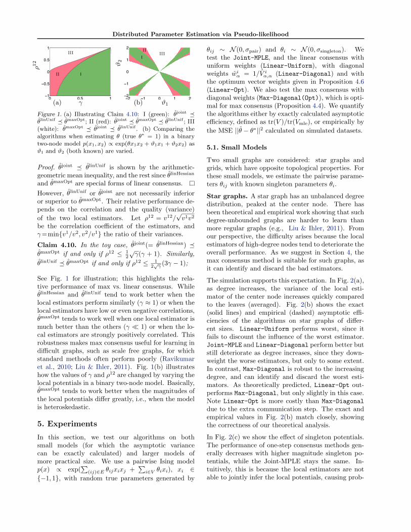
Figure 1. (a) Illustrating Claim 4.10: I (green): θjoint �θlinUnif � θmaxOpt; II (red): θjoint � θmaxOpt � θlinUnif ; III(white): θmaxOpt � θjoint � θlinUnif . (b) Comparing thealgorithms when estimating θ (true θ∗ = 1) in a binarytwo-node model p(x1, x2) ∝ exp(θx1x2 + ϑ1x1 + ϑ2x2) asϑ1 and ϑ2 (both known) are varied.

Proof. θjoint � θlinUnif is shown by the arithmetic-geometric mean inequality, and the rest since θlinHessian

and θmaxOpt are special forms of linear consensus.

However, θlinUnif or θjoint are not necessarily inferioror superior to θmaxOpt. Their relative performance de-pends on the correlation and the quality (variance)

of the two local estimators. Let ρ12 = v12/√v1v2

be the correlation coefficient of the estimators, andγ=min{v1/v2, v2/v1} the ratio of their variances.

Claim 4.10. In the toy case, θjoint(= θlinHessian) �θmaxOpt if and only if ρ12 ≤ 1

2

√γ(γ + 1). Similarly,

θlinUnif � θmaxOpt if and only if ρ12 ≤ 12√γ (3γ − 1);

See Fig. 1 for illustration; this highlights the rela-tive performance of max vs. linear consensus. WhileθlinHessian and θlinUnif tend to work better when thelocal estimators perform similarly (γ ≈ 1) or when thelocal estimators have low or even negative correlations,θmaxOpt tends to work well when one local estimator ismuch better than the others (γ � 1) or when the lo-cal estimators are strongly positively correlated. Thisrobustness makes max consensus useful for learning indifficult graphs, such as scale free graphs, for whichstandard methods often perform poorly (Ravikumaret al., 2010; Liu & Ihler, 2011). Fig. 1(b) illustrateshow the values of γ and ρ12 are changed by varying thelocal potentials in a binary two-node model. Basically,θmaxOpt tends to work better when the magnitudes ofthe local potentials differ greatly, i.e., when the modelis heteroskedastic.

5. Experiments

In this section, we test our algorithms on bothsmall models (for which the asymptotic variancecan be exactly calculated) and larger models ofmore practical size. We use a pairwise Ising modelp(x) ∝ exp(

∑(ij)∈E θijxixj +

∑i∈V θixi), xi ∈

{−1, 1}, with random true parameters generated by

θij ∼ N (0, σpair) and θi ∼ N (0, σsingleton). Wetest the Joint-MPLE, and the linear consensus withuniform weights (Linear-Uniform), with diagonalweights wiα = 1/V iα,α (Linear-Diagonal) and withthe optimum vector weights given in Proposition 4.6(Linear-Opt). We also test the max consensus withdiagonal weights (Max-Diagonal(Opt)), which is opti-mal for max consensus (Proposition 4.4). We quantifythe algorithms either by exactly calculated asymptoticefficiency, defined as tr(V )/tr(Vmle), or empirically by

the MSE ||θ − θ∗||2 calculated on simulated datasets.

5.1. Small Models

Two small graphs are considered: star graphs andgrids, which have opposite topological properties. Forthese small models, we estimate the pairwise parame-ters θij with known singleton parameters θi.

Star graphs. A star graph has an unbalanced degreedistribution, peaked at the center node. There hasbeen theoretical and empirical work showing that suchdegree-unbounded graphs are harder to learn thanmore regular graphs (e.g., Liu & Ihler, 2011). Fromour perspective, the difficulty arises because the localestimators of high-degree nodes tend to deteriorate theoverall performance. As we suggest in Section 4, themax consensus method is suitable for such graphs, asit can identify and discard the bad estimators.

The simulation supports this expectation. In Fig. 2(a),as degree increases, the variance of the local esti-mator of the center node increases quickly comparedto the leaves (averaged). Fig. 2(b) shows the exact(solid lines) and empirical (dashed) asymptotic effi-ciencies of the algorithms on star graphs of differ-ent sizes. Linear-Uniform performs worst, since itfails to discount the influence of the worst estimator.Joint-MPLE and Linear-Diagonal perform better butstill deteriorate as degree increases, since they down-weight the worse estimators, but only to some extent.In contrast, Max-Diagonal is robust to the increasingdegree, and can identify and discard the worst esti-mators. As theoretically predicted, Linear-Opt out-performs Max-Diagonal, but only slightly in this case.Note Linear-Opt is more costly than Max-Diagonal

due to the extra communication step. The exact andempirical values in Fig. 2(b) match closely, showingthe correctness of our theoretical analysis.

In Fig. 2(c) we show the effect of singleton potentials.The performance of one-step consensus methods gen-erally decreases with higher magnitude singleton po-tentials, while the Joint-MPLE stays the same. In-tuitively, this is because the local estimators are notable to jointly infer the local potentials, causing prob-


2 4 6 8 100

20

40

60

Tra

ce o

f Asy

mpt

otic

Var

ianc

e

Number of Nodes

The centerThe leaves

2 4 6 8 100.8

0.85

0.9

0.95

1

Number of NodesA

sym

ptot

ic E

ffici

ency

0.5 1 1.50.5

0.6

0.7

0.8

0.9

1

σsingleton

Asy

mpt

otic

Effi

cien

cy (

Exa

ct)

50 100 250 500 10008

10

12

14

16

18

Sample Size

n||θ

−θ∗||2

MLEJoint−MPLELinear−OptLinear−UniformLinear−DiagonalMax−Diagonal (Opt)

(a) σpair = σsingleton = .5 (b) σpair = σsingleton = .5 (c) σpair = .5 (d) σpair = σsingleton = .1

Figure 2. Results on star graphs. (a) Variance is much higher at the hub than at the leaves. (b) Exact (solid lines) andempirical (dashed lines) asymptotic efficiency of various algorithms vs. the size of the star graph. (c) The exact asymptoticefficiency for a 10-node star with σpair = 0.5 and σsingleton ∈ [.5, 2]. (d). The mean square error vs. the number of dataon a 10-node star graph; All the results are averaged on 50 random models, each with 50 random datasets.

lems when those local potentials dominate. Since ouranalysis is mainly asymptotic, we evaluate how the al-gorithms perform for small sample sizes in Fig. 2(d).As can be seen, the finite sample performance is es-sentially consistent with the asymptotic analysis.

4×4 Grid. The algorithms’ performance on gridshave the opposite trends; see Fig. 3(a). Joint-MPLE

performs best, while max-Diagonal performs rela-tively poorly. This is because grids have balanced de-gree, and all the local estimators perform equally well.We check the finite sample performance of the algo-rithms in Fig. 3(b), which again shows similar trendsto our asymptotic results. Finally, we show the con-vergence of ADMM in Fig. 3(c), illustrating that ourinitialization increases the convergence speed greatly.

5.2. Larger Models

We also test our algorithms on larger graphs, includ-ing a 100-node scale free network generated via theBarabasi-Albert model (Barabasi & Albert, 1999) anda 100-node Euclidean graph generated by connectingnearby sensors (distance ≤ .15) uniformly placed onthe [0, 1]× [0, 1] plane; see Fig. 4. On these models, weestimate both the singleton and pairwise parameters.In Fig. 4(a)-(b) we see trends similar to their smalleranalogues, the star graph and 4×4 grid, verifying thatour analysis remains useful on models of larger sizes.

6. Related Work

A very recent, independently developed work (Wiesel& Hero, 2012) adopts a similar, but less general ap-proach for Gaussian covariance estimation. They pro-pose a similar linear consensus approach (using onlyuniform weights) and a similar parallel algorithm forjoint MPLE, but do not discuss max consensus or lin-

ear consensus with general weights, and do not pro-vide a comprehensive theoretical analysis. Anotherrecent work (Eidsvik et al., 2010) uses composite like-lihood for parallel computing on spatial data. Bradley& Guestrin (2011) gave a sample complexity analysisfor MPLE and disjoint MPLE, which may be extensi-ble to our algorithms.

Another line of work approximates MLE by estimat-ing the partition function with variational algorithms(e.g., Wainwright, 2006; Sutton & McCallum, 2009).These methods can perform well at prediction taskseven with a “wrong” model, and can take a message-passing form potentially suitable to distributed set-tings. However, in terms of parameter estimation,these methods introduce a bias due to the approxi-mate inference that is hard to estimate or control.

7. Conclusion

In this work, we present a general framework for dis-tributed parameter learning. We show that the smartone-step consensus methods of the local estimators,especially those that exploit local second-order infor-mation, are both computationally efficient and statis-tically competitive with iterative methods using jointoptimization. Particularly, we show that the max com-bination method is well suited to scale-free networks, awell-identified problem for existing methods. Our the-ory of combining estimators is quite general, and canbe applied to other contexts to boost statistical per-formance. Future directions include considering modelmisspecification, finite sample complexity analysis andextension to high-dimensional structure learning.

Acknowledgements. Work supported in part byNSF IIS-1065618 and a Microsoft Research Fellowship.


0 0.5 10.65

0.7

0.75

0.8

0.85

0.9

σsingleton

Asy

mpt

otic

Effi

cien

cy (

Exa

ct)

50 100 20020

30

40

50

60

Sample Size

n||θ

−θ∗||2


0 10 20 30 40 5039

40

41

42

43

44

Iteration

n||θ

−θ∗||2

Initial−ZeroLinear−UniformLinear−Diagonal

(a) σpair = .5 (b) σpair = σsingleton = .1 (c) σpair = σsingleton = .5

Figure 3. Results on 4 × 4 grid. (a) Exact asymptotic efficiency of the algorithms when σsingleton ∈ [0, 1]. (b) EmpiricalMSE vs. data size. Solid horizontal lines show the theoretical asymptotic MSEs. (c) Convergence of ADMM, initializedat zero with ρiα = 1 (yellow), and initialized to linear consensus estimates with uniform (red) or diagonal (green) weights,with ρiα set to the corresponding weights. All results are averaged on 50 random models with 50 datasets each.

200 1000 5000 50000200

210

220

230

240

250

Sample Size

n||θ

−θ∗||2

200 1000 5000 50000

380

400

420

440

460

Sample Size

n||θ

−θ∗||2


(a) scale-free graph, σpair = σsingleton = .1 (b) Euclidean graph, σpair = σsingleton = .1

Figure 4. The empirical mean square error vs. the sample sizes on (a) a 100-node scale-free network and (b) a 100-nodeEuclidean graph. The results are averaged on 5 sets of random models and then 50 datasets, and show similar relativeperformance trends to the small-scale experiments.

References

Barabasi, A.-L. and Albert, R. Emergence of scaling inrandom networks. Science, 286(5439):509–512, 1999.

Bertsekas, D. and Tsitsiklis, J. Parallel and distributedcomputation: numerical methods. Prentice-Hall, 1989.

Besag, J. Statistical analysis of non-lattice data. J. RoyalStat. Soc. D, 24(3):179–195, 1975.

Boyd, S., Parikh, N., Chu, E., Peleato, B., and Eckstein,J. Distributed optimization and statistical learning viathe alternating direction method of multipliers. Found.Trends in Machine Learn., 3(1):1–122, 2011.

Bradley, J. K. and Guestrin, C. An asymptotic analysis ofgenerative, discriminative, and pseudolikelihood estima-tors. In AISTATS, 2011.

Cetin, M., Chen, L., Fisher III, J., Ihler, A., Kreidl, O.,Moses, R., Wainwright, M., Williams, J., and Willsky,A. Graphical models and fusion in sensor networks.Wireless Sensor Networks, pp. 215–249, 2007.

Eidsvik, J., Shaby, B. A., Reich, B. J., Wheeler, M., andNiemi, J. Estimation and prediction in spatial modelswith block composite likelihoods using parallel comput-ing. in submission, NTNU, Duke, NCSU, UCSB, 2010.

Godambe, V. P. An optimum property of regular maxi-mum likelihood estimation. Ann. Math. Stat., 31(4):pp.

1208–1211, 1960.Liang, P. and Jordan, M.I. An asymptotic analysis of gen-

erative, discriminative, and pseudolikelihood estimators.In ICML, pp. 584–591, 2008.

Lindsay, B.G. Composite likelihood methods. Contempo-rary Mathematics, 80(1):221–39, 1988.

Liu, Q. and Ihler, A. Learning scale free networks byreweighted L1 regularization. In AISTATS, pp. 40–48.2011.

Ravikumar, P., Wainwright, M. J., and Lafferty, J. High-dimensional Ising model selection using L1-regularizedlogistic regression. Ann. Stat., 38(3):1287–1319, 2010.

Sutton, C. and McCallum, A. Piecewise training for struc-tured prediction. Mach. Learn., 77(2–3):165–194, 2009.

van der Vaart, A. Asymptotic statistics. Cambridge, 1998.Wainwright, M. Estimating the wrong graphical model:

Benefits in the computation-limited setting. J. MachineLearn. Res., 7:1829–1859, 2006.

Wainwright, M. and Jordan, M. Graphical models, ex-ponential families, and variational inference. Found.Trends Mach. Learn., 1(1-2):1–305, 2008.

Wiesel, A. and Hero, A.O. Distributed covariance estima-tion in Gaussian graphical models. IEEE Trans. Sig.Proc., 60(1):211–220, January 2012.

distributed parameter estimation via pseudo-likelihood · let sbe a ran- dom vector with s ......

Documents