distributed global id assignment for wireless...

Distributed Global ID Assignment for Wireless SensorNetworks ∗

ElMoustapha Ould-Ahmed-Vall, Douglas M. Blough, Bonnie Heck Ferri, George F. Riley

School of Electrical and Computer Engineering, Georgia Institute of TechnologyAtlanta, GA 30332-0250

{eouldahm,doug.blough,bonnie.heck,riley}@ece.gatech.edu

Abstract

A sensor network consists of a set of battery-powered nodes, which collaborate to perform sens-ing tasks in a given environment. It may contain one or more base stations to collect sensed dataand possibly relay it to a central processing and storage system. These networks are characterized byscarcity of resources, in particular the available energy.

We present a distributed algorithm to solve the unique ID assignment problem. The proposed so-lution starts by assigning long unique IDs and organizing nodes in a tree structure. This tree structureis used to compute the size of the network. Then, unique IDs are assigned using the minimum num-ber of bytes. Globally unique IDs are useful in providing many network functions, e.g. configuration,monitoring of individual nodes, and various security mechanisms.

Theoretical and simulation analyses of the proposed solution have been performed. The resultsdemonstrate that a high percentage of nodes (more than 99%) are assigned globally unique IDs atthe termination of the algorithm when the algorithm parameters are set properly. Furthermore, thealgorithm terminates in a relatively short time that scales well with the network size.

1 Introduction

A sensor network consists of a set of battery-powered nodes, which collaborate to perform sensing tasksin a given environment. It may contain one or more base stations to collect sensed data and possiblyrelay it to a central processing and storage system.

The communication range of individual sensor nodes is generally limited, and communication is oftencarried out in a multi-hop manner. There is a need to have a unique identifier in the header of everyunicast packet. In fact, routing protocols need to uniquely identify the final destination as any node inthe network can be a potential destination. Several routing protocols use attribute-based routing andtherefore can use attributes as global identifiers. However, even these protocols require the existence ofunique IDs at a local level. This is the case for directed diffusion [1] and geographical routing protocols

∗This work is supported in part by NSF under contract numbers ANI-9977544, ANI-0136969, ANI-0240477, ECS-0225417, CNS 0209179, and DARPA under contract number N66002-00-1-8934.

1

such as [2]. Network-wide unique IDs are beneficial for administrative tasks requiring reliability, suchas configuration and monitoring of individual nodes, and download of binary code or data aggregationdescriptions to sensor nodes [3]. Network-wide unique IDs are also required when security is neededin sensor networks [4]. Several MAC protocols requiring the preexistence of network-wide unique IDshave also been proposed for sensor networks [5].

Assumption of the preexistence of network-wide IDs is not realistic in the case of sensor networks.The preexistence of network-wide global IDs requires hard-coding these IDs on nodes prior to the de-ployment. This is costly in terms of time and effort when a network contains thousands to hundreds ofthousands of nodes. Another alternative is to have MAC addresses that are unique for every manufac-tured sensor node, as is the case for Ethernet cards [6]. This is not a desirable approach because of thecoordination it requires and the fact these IDs would have to be lengthy and therefore costly to use inpacket headers.

An obvious ID assignment strategy is to have each node randomly choose an ID such that the prob-ability of any two nodes choosing the same ID is very low. However, for this probability to be low, weneed the IDs to be very long, which is again costly in terms of energy [7]. Any ID assignment solutionshould produce the shortest possible addresses because sensor networks are energy-constrained. Theusage of the minimum number of bytes required is motivated by the need to limit the size of transmittedpackets, in particular the header. In fact, communication is usually the main source of energy drain in asensor node [8]. For this reason, sensor networks are designed to limit the amount of data transmitted,for example through data aggregation. This reduces the payload of transmitted packets, which makesthe header size even more significant.

In this paper, we introduce an algorithm that assigns unique IDs to sensor nodes using only the mini-mum number of bytes required to assign each node in the network a unique ID. The algorithm does notassume the pre-existence of any type of identification and scales well with the size of the network. Wealso do not assume the existence of any specific communication protocol. In particular, the preexistenceof a specific collision avoidance mechanism is not assumed. The algorithm handles collisions throughavoidance and recovery. Collisions are avoided through the scheduling of transmissions at random times.If collisions occur, they are detected through a confirmation mechanism, and recovery is performed byretransmitting colliding packets. Our algorithm can handle the case of asynchronous wake-up. Nodescan join the network after the execution of the algorithm and still obtain a unique ID in an energy ef-ficient manner. The handling of asynchronous wake-up is particularly important in the case of sensornetworks where many nodes may be in a sleep state during the initialization phase for the purpose ofenergy saving and network lifetime optimization [9].

The algorithm can be divided into three main phases. In the first phase, a tree structure is establishedand, at the same time temporary long IDs are assigned. These temporary IDs are used for reliablecommunication during the remaining two phases. In the second phase, the size of sub-trees is reportedbottom-up from leaf nodes to the root. In the third phase, the final short IDs are assigned. Each nodeparticipating in the initial phase of the algorithm requests additional spare IDs that are used to locallyassign unique IDs to neighboring nodes that asynchronously join the network.

We analytically prove the correctness and termination of the algorithm. We also assess its performancein terms of the execution time and the probability that a node is left without an assigned ID at the end ofthe algorithm.

It must be noted that a shorter paper describing an initial version of the proposed algorithm was pub-lished in [10]. The main differences between the two papers are the addition in this paper of the extension

2

of the algorithm to handle nodes that join the network in an asynchronous manner, and inclusion of amore comprehensive set of simulation results of the algorithm.

The rest of the paper is organized as follows. The related work is discussed in Section 2. In Section 3,the proposed algorithm is discussed for the case of sensor networks with synchronized deployment. Thetheoretical analysis of the proposed algorithm is presented in Section 4. Section 5 discusses extensivesimulation results of the algorithm. The algorithm is extended in Section 6 to handle the case of sensornetworks with asynchronous deployment. Section 7 presents simulation results for the extended algo-rithm. Section 8 discusses the costs and benefits of using our ID assignment algorithm. The paper isconcluded in Section 9.

2 Related Work

In general, network-wide unique addresses are not needed to identify the destination node of a specificpacket in sensor networks. In fact, attribute-based addressing fits better with the specificities of sensornetworks [11]. In this case, an attribute such as node location and sensor type is used to identify thefinal destination. However, different nodes can have the same attribute value, in particular in the sameneighborhood. Thus, there is a need to uniquely identify the next hop node during packet routing [12].Furthermore, it is possible that two neighboring nodes have the same attributes. For instance, it is likelythat some nodes will have the same location in a dense sensor network. In addition, the number of bitsrequired to represent attribute information (for example the node geographical coordinates) may be largerendering this approach less attractive from a communication energy point of view [13].

In [14], the authors propose an algorithm that assigns globally unique IDs. Like our algorithm, it usesa tree structure to guarantee the uniqueness of each ID. The algorithm is similar to the first phase ofour algorithm. It starts with the sink node broadcasting a message that contains its ID and a parameterb given the size in bits of one-hop ID. Successive nodes choose a parent node among their neighborsthat already have an ID. The node then randomly chooses an ID of size b bits and relays on its parentto guarantee no other node has chosen the same ID. The node then appends its chosen ID to the ID ofits parent to create a unique ID. The main difference between this algorithm and ours is that it doesnot use the network size to minimize the size of node IDs. Our algorithm, in contrast, not only assignsunique IDs but also guarantees that these IDs are of minimum length. This is is a considerable advantageconsidering that sensor networks are energy-sensitive.

Several schemes have been proposed to assign locally unique addresses in sensor networks. In [8],Schurgers, et al., developed a distributed allocation scheme where local addresses are spatially reused toreduce the required number of bits. The preexisting MAC addresses are converted into locally uniqueaddresses. Each locally unique address is combined with an attribute-based address to uniquely deter-mine the final destination of a packet. This use of locally unique addresses instead of global addressesdoes not affect the operations of the existing routing protocols. This solution assumes the preexistenceof globally unique addresses, which our algorithm does not assume. Our solution can be used to assignthese global addresses prior to use of the method in [8]. Our proposed solution allows for asynchronouswake-up. When a new node joins the network, it chooses a random address and shares it with its neigh-bors. The neighbors compare the new address with the addresses of other neighbors to detect and resolveany conflicts.

In [12], Ali, et al., proposed an addressing scheme for cluster-based sensor networks [15]. To prevent

3

collisions, nodes within the same cluster are assigned different local addresses. Non-member one-hopand two-hop neighbors must also have different local addresses to avoid the hidden-terminal problem.The network is divided into hierarchical layers where the number of layers increases with the number ofnodes in the network. Global IDs are obtained by concatenating the local address and the addresses ofthe head nodes of the different layers. This solution suffers from the fact that the address size increaseswith the number of layers as 6 bits are added for each layer. This makes this solution less attractive dueto the energy cost of using global IDs in the case of large sensor networks. In addition, this solution canbe used only with cluster-based routing and does not extend to the case of multi-hop routing [16].

In [3], Dunkels, et al., developed a spatial IP addressing scheme using node location. The (x, y) coor-dinates of a node are used as the two least significant bytes of its spatial IP. This solution is particularlyattractive since it can facilitate the interaction between sensor networks and other types of networks.However, it also suffers from the large size of generated addresses leading to higher overhead. It alsorequires the existence of a localization mechanism since it assumes that nodes are location-aware.

In [13], the authors propose a local ID assignment scheme where address conflicts are resolved in areactive way. Nodes randomly choose an address that is likely to be unique within a 2-hop neighborhood.No conflict resolution is performed until nodes need to enter in a communication. For instance, interestbroadcasting in directed diffusion can be used to resolve conflicts. In this case, the sink node discoversthe existence of identical IDs between its immediate neighbors. The conflicting nodes are notified andchoose new IDs. Each node that forwards the interest message uses the response messages to detect IDconflicts among its neighbors. The delaying can help save energy by avoiding any unnecessary conflictresolution. In particular, if two neighbors have the choose the same local ID but are never active atthe same time, resolving such a conflict amounts to a waste of energy resources. However, resolvingID conflicts reactively can be problematic if the sensor network requires time-sensitive exchange ofinformation, since messages can be delayed to resolve an ID conflict.

In [17], Motegi et al. propose an on-demand address scheme. To reduce the number of bits required torepresent addresses and the number of control messages needed to establish these addresses, the authorspropose to assign temporary addresses to nodes detecting an event on an on-demand basis. When a nodebecomes active (detects an event), it chooses a random network-wide ID and sends a route request tothe sink node using the AODV protocol [18]. The intermediate and the sink node perform a conflictresolution. Once the node communication with the sink node terminates (the node is no longer active),its address goes back to the free address pool and can be used by newly active nodes. This approachcan effective reduce the number of bits required for globally unique IDs. However, it assumes the pre-existence of some of form of network-wide unique IDs (e.g., MAC or IP addresses). The pre-existingaddresses are needed to establish locally unique and permanent addresses used by the proposed algorithmfor neighbor identification and collision avoidance.

In [19], the authors present the GREENWIS algorithm designed to assign group IDs. The objective isto assign group IDs rather than individual node IDs. Neighboring nodes share the same group ID, whichallows the number of bits required to represent each to be much smaller. The main problem with thisapproach is that it can be used to provide functionalities such as collision avoidance as all neighbors areassigned the same ID.

The ID assignment problem is related to the overall sensor network initialization. Initialization canbe viewed as the mechanism needed for individual sensor nodes to become an integral part of a sensornetwork. When a sensor network is initially deployed, there is no established structure to allow nodes toefficiently communicate [9]. The initialization has the objective of transitioning from this unstructured

4

state to a structured network and the establishment of a MAC protocol to allow efficient informationdissemination. An important way to structure sensor nodes into a network is through the use of clusteringtechniques [20, 21, 9]. Many of the clustering algorithms that have been proposed for sensor networksassume the pre-existence of unique node IDs. For example, in the approach proposed in [9] a newlyactive node that wants to join the network waits for messages from neighboring dominators (clusterheads) before trying to become a dominator. A unique ID is needed to distinguish between the differentdominators in the neighborhood. The ID assignment algorithm proposed here can be used as part ofthe overall network initialization phase. In this way, the initialization does not need to require the pre-existence of node IDs. Like the work in [9], our approach does not assume that all nodes wake-up at thesame time. We also do not assume the existence of a specific collision avoidance protocol.

3 Unique ID Assignment Algorithm

We present a distributed algorithm that assigns globally unique IDs to sensor nodes. Initially, we assumethat all nodes are awake during the execution of the algorithm. This assumption is relaxed later in thispaper to accommodate a dynamic network where nodes can join the network at any time during theinitial execution of the algorithm or after its termination. The algorithm can be divided into three mainphases. In the first phase, the objective is to assign temporary unique identifiers in the form of potentiallylong vectors of bytes. A tree structure rooted at the node initiating the algorithm is established duringthis phase. The main difficulty here is to guarantee the uniqueness of the assigned IDs and to minimizecost by controlling the probability of message collisions.

In the second phase, the temporary identifiers are used to reliably compute the size of each sub-treeand report it to the parent node. This process is done for each sub-tree from leaf nodes until the rootnode. At the end of this phase, the initiator knows the total size of the network. This allows the initiatorto compute the minimum number of bytes required to give a unique ID to each node in the tree.

The third phase consists of assigning final IDs to each node in the network going from the root to theleaf nodes. In this phase as in the previous one, it is necessary to control the parameters of the algorithmto minimize the communication energy cost while keeping the execution time of the algorithm short.

These different phases are now described in detail.

3.1 Phase 1: Tree Building and Temporary ID Assignment

In this phase, temporary IDs are assigned and a tree structure is established. The temporary ID of aparticular node is a vector of bytes that uniquely identifies it. The temporary ID of a child node has onebyte more than that of its parent. We assume a network density, such that no node has more than 256neighbors. However, for networks of higher density, temporary IDs can be modified to be vectors withelements of 2 or 3 bytes as needed. The algorithm starts with the initiator node, typically the base station,choosing its temporary ID to contain one byte of value 0, and broadcasting an initialization message oftype 1. Each node receiving an initialization message for the first time considers its parent to be thesender of the message and initializes its temporary ID to that of its parent node.

The receiving node then chooses a 4-byte integer unfirormly at random and prepares a message of type2 to send to its parent node. This message also contains a retry counter. The sending of this message isscheduled at a random time uniformly distributed between timeWait and 2 × timeWait from the time

5

of reception of the initialization message to avoid collision with messages sent by other children. Uponreception of a new message of type 2, the parent node checks if any other child node had already chosenthe same random number. If so, a reinitialization message of type 3 is immediately sent to the child node.If no other child had chosen the same number, the parent node immediately sends a message containingan assigned ID of one byte that is different from the ones sent to other children nodes. This messageis of type 4. The reception of this message is immediately confirmed to the parent by a confirmationmessage of type 5.

After receiving the message of type 4 containing the 1-byte unique child ID, this byte is added atthe end of the temporary ID. The child node then schedules the sending of an initialization message atrandom time uniformly distributed between timeWait and 2× timeWait from the time of reception ofthe type 4 message. At the scheduled time, the node sends an initialization message of type 1 and waitsfor a certain amount of time (5 × timeWait) to hear from any potential children. If any child respondswithin this period, the previous procedure of assigning one byte ID repeats itself. If no child responds,the node considers itself a leaf node.

All messages except the ones of type 1 are exchanged in a reliable way. A message of type 2, whichcontains the random 4-byte integer chosen by a child node, is confirmed by the reception of a messageof type 3 (reinitialization message) or type 4 (containing a 1-byte assigned ID). A message of type 3 isresent if the parent node receives a second message of type 2 with the same 4-byte ID. A message of type4 is confirmed through the reception of the confirmation message of type 5. If a message is not confirmedwithin a random period chosen uniformly between timeWait and 2× timeWait, the message is resent.The node keeps checking for a confirmation and resending until the message is confirmed.

Figure 1 illustrates the messages exchanged between a parent node and a child node during phase 1when no reinitialization message is sent. A reinitialization message makes the child node resends themessage of type 2. At the end of this exchange, the child node has a temporary ID that is 1 byte longerthan the one of its parent node. The child node then sends its own message of type 1. Algorithm 3.1 givesthe pseudo code of the first phase. Note that at the end of this phase every node knows the temporary IDof its parent node. The parent ID is equal to the node ID without the last byte.

3.2 Phase 2: Collecting the Sub-Tree Sizes

In this phase, nodes report their sub-tree sizes from the leaf nodes to the root node. The sub-tree sizeof a particular node is the number of nodes contained in the tree rooted at that node at the end of phase1. A node that is declared a leaf at the end of phase 1 considers its sub-tree size to be 1 and sends it asa message of type 6 to its parent. A non-leaf node waits until it receives sub-tree sizes from all of itschildren nodes before sending its sub-tree size to its parent. Sub-tree size messages are confirmed bythe parent node with a confirmation message of type 7. Figure 2 illustrates the message exchange duringphase 2 to collect the sub-tree sizes.

When the initiator receives sub-tree size messages from all of its children, it knows the total numberof nodes in the network. This total is used to compute the minimum number of bytes needed to codea unique final ID for each node in the network. These IDs are assigned in phase 3 of the algorithm.Algorithm 3.2 gives the pseudo code of the second phase. Note that at the end of this phase every nodeknows its sub-tree size as well as the sub-tree size of each of its children nodes.

6

PSfrag replacements

Parent node

Child nodetype

1,t0

type

2,t1

type4,t2

type

5,t3

TempID: 163.25

TempID: 163.25.41

Figure 1: One step of phase 1 with no reinitialization message

3.3 Phase 3: Final Unique ID Assignment

In this phase, the final unique IDs are assigned by each parent node to its children nodes starting fromthe root. Final IDs are coded using the same number of bytes for all nodes. The initiator is assigned anID of 0. It sends a final ID message (message of type 8) to each of its children nodes. Each messagecontains a unique ID and the number of bytes to be used to code IDs. Final ID messages are confirmedwith messages of type 9. Each node receiving a message of type 8 takes the ID it contains as its final IDand knows that a number of IDs starting from its ID and containing as many IDs as needed is reservedfor the IDs of the nodes in its sub-tree. Each non-leaf node receiving a final ID message confirms it andassigns IDs to its children nodes in a similar way.

Figure 3 illustrates the message exchange during phase 3 to allocate the final IDs. Each node allocatesits ID plus 1 to its first child and then allocates IDi to the ith child with IDi+1 = IDi + Si, where Si isthe sub-tree size of the ith child. Algorithm 3.3 gives the pseudo code of the third phase. At the end ofthis phase, every node in the network knows its final ID. These final IDs are coded using the minimumnumber of bytes.

3.4 Collision Handling

Assuming a single channel, if a node ns is transmitting a message to a node nr, a collision occurs ifnr is already in the process of receiving from a different node. The algorithm does not assume the

7

Algorithm 1 Phase 1: Temporary ID AssignmentChildB := 1

idConfirmed := false

if initiator is true thentempId := 0

send an initialization message of type 1end ifif receive message msg of type 2 then

if a child already have same intId thensend reinitialization message of type 3

end ifif no child already has same intId then

add to children listchoose a random time rtschedule checking for confirmation at rtsend message of type 4 with ChildIdBChildIdB := ChildIdB + 1

end ifend ifif receive msg message of type 5 then

if msg.dest = tempId thenfind ch, the corresponding childch.tempIdConfirmed := true

ch.sizeReceived := false

end ifend ifif receive first message msg of type 1 then

idAssigned := true

tempId := msg.source

choose a random 4-byte intId

choose a random time rt

schedule checking for confirmation at rt

send message of type 2 with intId

end ifif receive msg message of type 3 then

choose a different random 4-byte intId



send message of type 2 with intId


if idConfirmed is true thenupdate timeWait

resend message of type 5end ifif idConfirmed is not true then

update tempId and idConfirmed

update timeWait


schedule sending message of type 1 at rt

send message of type 5end if

end if

existence of any specific MAC protocol. In particular, no collision avoidance mechanism is required.Collision is handled in the sense that all messages except the initialization message (message of type1) received by a node are confirmed by an acknowledgment message. Before sending a message, anode chooses randomly an integer number rn between 0 and RANDMAX , and waits for a time equalto (1 + rn ÷ RANDMAX) × timeWait. If it does not receive the confirmation within the randomwaiting time, it resends the message and keeps doing so until receiving the confirmation.

The node adapts the parameter timeWait to the traffic condition. In fact, this parameter is increased

8

PSfrag replacementstyp

e 6,t0

type7,t1

type

6,t2

type7,t3

type6,

t4

type 7, t5

type

6,t6

type7,t7

TempID: 41.62.1

TempID: 41.62.0

TempID: 41.62.2

TempID: 41.62

TempID: 41

Size: 300

Size: 100

Size: 1

Size: 402

Size: 403

Figure 2: One step of phase 2

by half of its initial value (timeWaitI) every time an expected confirmation is not received, unlesstimeWait has already reached an upper limit set to 5 × timeWaitI . Upon the reception of a message,timeWait is reduced by half of timeWaitI , unless a lower bound, set to the initial value, is alreadyreached.

For the message of type 1, it is assumed that every node has several neighbors. Each neighbor sends aninitialization message at a different time (randomly chosen after the first phase) to reduce the probabilityof collision. Therefore, a node has several possibilities of receiving an initialization message.

4 Theoretical Analysis

This section contains the theoretical evaluation of the unique ID assignment algorithm. In particular, thecorrectness of the algorithm is analyzed. We also prove that the algorithm terminates naturally and givean upper limit on the average energy consumption per node. Since the initial assignment messages (of

9

Algorithm 2 Phase 2: Sub-tree Sizes CollectingsubtreeSize := 1

sizeConfirmed := false

if receive msg message of type 6 thenfind ch, the corresponding childif ch.sizeReceived is true then

resend message of type 7end ifif ch.sizeReceived is not true then

ch.subtreeSize and ch.sizeConfirmed

subtreeSize := subtreeSize + ch.subtreeSize

send message of type 7choose a random time rt

schedule checking if all sub-tree sizes received at rt

end ifend ifif leaf is true then



send message of type 6end ifif receive msg message of type 7 then

if sizeConfirmed is not true thenupdate sizeConfirmed

end ifend ifif sub-tree size messages received from all children and initiator is not true then



send message of type 6end if

type 1) are sent unreliably, we also analyze the probability of a node being left out by the algorithm.Such a node does not participate in the algorithm and is not assigned an ID.

In this section, we study the case of a synchronized wake-up where all nodes composing the networkparticipate in the initial phase of the algorithm. In particular, the following properties are assumed. Thecase of asynchronous wake-up is handled in Section 6 later in the paper.

Assumption 1. All nodes are assumed to be awake during the initial phase of the algorithm.

This assumption implies that no node is allowed to join the network after the initial phase of thealgorithm. A node joining the network after all messages of type 1 have been sent by its neighborscannot participate in the algorithm and will not receive an ID.

Assumption 2. All nodes that participate in the initial phase of the algorithm are assumed to remainactive and maintain parent-child node connectivity until the termination of the algorithm.

This assumption is needed to avoid a parent or a child node waiting indefinitely for a message froma node that is no longer active. The primary failure mode we consider in this work is node death due toenergy depletion. As is shown later in the theoretical and simulation analyses, the initialization algorithmterminates in a short time, as compared to the average lifetime of a node. Therefore, Assumption 2is very unlikely to be violated due to nodes dying. Another possible way in which this assumptioncould be violated is due to drastic changes in environmental (e.g. terrain) conditions that would causesome communication links to be lost. We assume that this situation is fairly rare and handle it in theasynchronous wakeup discussing in Section 6.

10

SubT5

PSfrag replacements

type8,t4

type 9,

t5

type8,t2

type

9,t3

type 8, t6

type9

,t7

type8,t0

type

9,t1

FinalID: 200

FinalID: 100

FinalID: 500

FinalID: 99

FinalID: 98

Size: 300

Size: 100Size: 1

Size: 402

Size: 403

Figure 3: One step of phase 3

The two assumptions above are necessary primarily for the formal proof of correctness that followsin this section. Both of these assumptions are relaxed in Section 6.

4.1 Model

The evolution of each node, except for the initiator, is modeled as a stochastic process with state spaceof s = {0, 1, 2, 3, 4, 5}. The different states are defined as follows:

1. State 0: A node is in state 0 if it did not yet receive any initialization message (message of type 1).

2. State 1: A node is in state 1 if it has already received an initialization message, is still waiting forits temporary ID to be confirmed by its parent node.

11

Algorithm 3 Phase 3: Final IDs Assignmentif sub-tree size messages received from all children and initiator is true then

compute nbBytes, the number of bytesmyId := 0

idAssignedF := true

currentId := 1

choose random time rt


send message of type 8 to first child with currentId


find ch, the corresponding childif ch.idF inalConfirmed is true then

ignoreend ifif ch.idF inalConfirmed is not true then

ch.idF inalConfirmed := true

currentId := currentId + ch.subtreeSize

if more nodes in the children list thenchoose random time rt


send message of type 8 to next child with currentId

end ifend if


if idAssignedF is true thenresend final ID confirmation message of type 9

end ifif idAssignedF is not true then

idAssignedF := true

myId := msg.minId

currentId := myId + 1

send message of type 9 to parent nodechoose random time rt


send message of type 8 to first child with currentId

end ifend if

3. State 2: A node is in state 2 if its temporary ID has been confirmed by its parent node, but it didnot yet send a message of type 1.

4. State 3: A node is in state 3 if its temporary ID has been confirmed by its parent node, it has senta message of type 1, but did not yet send its sub-tree size message. This could be because it isstill waiting to know if it is a leaf, or is still waiting for at least one child node to report the size ofits sub-tree. It could also be during the period after receiving all sub-tree sizes, but the scheduledtime to send its sub-tree message has not been reached

5. State 4: A node is in state 4 if it has already reported its sub-tree size to its parent node but is stillwaiting to receive its final ID.

6. State 5: A node is in state 5 if it has already received its final ID.

Clearly, state 5 is a stable state after which the node does not go back to any other state. It is also clearthat a node can only go to the next higher state or remain in its current state. That is, for example, a nodein state 3 can only go to state 4 or remain in state 3. The probability that a node changes its state dependson its current state as well as the states of the neighboring nodes. In fact, the neighbors influence the

12

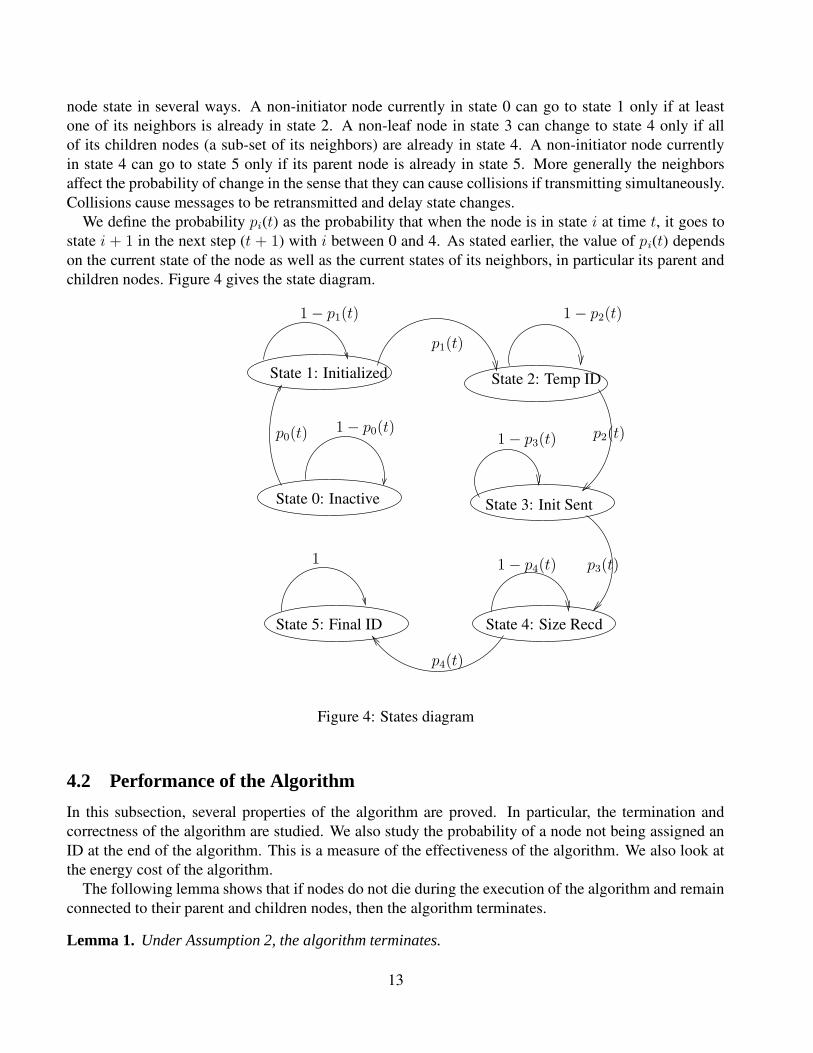
node state in several ways. A non-initiator node currently in state 0 can go to state 1 only if at leastone of its neighbors is already in state 2. A non-leaf node in state 3 can change to state 4 only if allof its children nodes (a sub-set of its neighbors) are already in state 4. A non-initiator node currentlyin state 4 can go to state 5 only if its parent node is already in state 5. More generally the neighborsaffect the probability of change in the sense that they can cause collisions if transmitting simultaneously.Collisions cause messages to be retransmitted and delay state changes.

We define the probability pi(t) as the probability that when the node is in state i at time t, it goes tostate i + 1 in the next step (t + 1) with i between 0 and 4. As stated earlier, the value of pi(t) dependson the current state of the node as well as the current states of its neighbors, in particular its parent andchildren nodes. Figure 4 gives the state diagram.

PSfrag replacements

State 0: Inactive

State 1: Initialized State 2: Temp ID

State 3: Init Sent

State 4: Size RecdState 5: Final ID

1 − p0(t)p0(t)

1 − p1(t)

p1(t)

1 − p2(t)

p2(t)1 − p3(t)

p3(t)1 − p4(t)

p4(t)

1

Figure 4: States diagram

4.2 Performance of the Algorithm

In this subsection, several properties of the algorithm are proved. In particular, the termination andcorrectness of the algorithm are studied. We also study the probability of a node not being assigned anID at the end of the algorithm. This is a measure of the effectiveness of the algorithm. We also look atthe energy cost of the algorithm.

The following lemma shows that if nodes do not die during the execution of the algorithm and remainconnected to their parent and children nodes, then the algorithm terminates.

Lemma 1. Under Assumption 2, the algorithm terminates.

13

Proof. The statement in this lemma is equivalent to declaring that any node reaching state 1 in the statesdiagram will eventually reach state 5 if no node dies during the algorithm execution and parent-childconnections are maintained. This is clearly the case when the probabilities p1(t), p2(t), p3(t), and p4(t)are each greater than 0. Each of these probabilities is permanently equal to 0 only if a neighboring nodewith which the node interacts in the current state (parent or child node) is no longer alive or can nolonger receives messages (e.g., change of terrain or new object between the two nodes causing loss ofconnectivity). In fact, if such a node dies or is no longer reachable, the dependent node can continuesending a message indefinitely while waiting for a confirmation. It can also indefinitely wait for a sizemessage (in case of parent node) or a final ID message (in a case of a child node). If no node in thenetwork dies or looses connection, each of the probabilities p1(t), p2(t), p3(t), and p4(t) does not remainequal to 0 all the time. Therefore, each node reaches the final state. The algorithm terminates when allleaf nodes reach the final state (state 5 in the states diagram).

Before studying the correctness of the algorithm, we look at the possibility of two nodes with thesame parent receiving the same temporary ID. This occurs only when two children of the same nodechoose the same 4-byte ID in first phase and respond simultaneously with messages of type 2 to theinitialization message and their parent receives only one of the two messages. For the two nodes to endup with the same temporary ID, they need also to send simultaneously the confirmation message of type5 and for their parent to receive one and only one of these messages.

We define Pi2 as the probability of two nodes having two identical temporary IDs. As we can see, Pi2

is very low because the occurrence of two nodes having two identical temporary IDs is conditioned onthe joint occurrence of a successive number of independent events each having a very low probability.In fact, Pi2 ≤ Pf ×Ps, where Pf is the probability of any two nodes in the network with the same parentchoosing the same 4-byte integer and Ps is the probability of the two nodes sending messages of type 2during the same time window. For a numerical example, let assume that each node has a radio with acapacity of 100 kbps and the each message of type 2 is no more than 25 bytes. It can easily be proventhat in this case, Ps ≤ (25 × 23) ÷ (100 × 210) = 1.95 × 10−3. It can also be proven that for a networkof n nodes each having no more than d = 50 neighbors, we have Pf ≤ (n × d) ÷ 232. For n = 10, 000,we obtain Pf ≤ 1.16 × 10−4. It follows that in this conservative example, Pi2 ≤ 2.27 × 10−7. In otherwords, the probability of any two nodes receiving the same ID is less than 1 in a million. The followinglemma states the correctness of the algorithm.

Lemma 2. Under Assumptions 1 and 2, each node receives a unique ID with a high probability of1 − Pi2, where Pi2 is as defined above.

Proof. The proof comes from the nature of the assignment of temporary and final IDs. Since temporaryIDs are assigned in a hierarchical way with children of same node all having different IDs, phase 1 endswith every node having a different temporary ID. The only exception is when two nodes receive the sametemporary ID. In phase 3, each parent node, starting from the initiator, reserves a different set of finalIDs for each of its children nodes having different temporary IDs to assign to its sub-tree. Therefore,every node having a unique temporary ID ends with a unique final ID. This proves the correctness of thealgorithm.

We now determine the probability that a message is successfully transmitted by the first trial and theprobability of reception by the second trial. A message is not successfully transmitted if a collision

14

occurs or a bit error prevents the successful interpretation of the message or the corresponding acknowl-edgment.

A collision is detected by the sender node, ns, when it does not receive the corresponding confirmationmessage in a randomly predetermined time period. As explained in Subsection 3.4, the length of this timeperiod is uniformly distributed between timeWait and 2 × timeWait. If no confirmation is received,the message is resent at the end of this period. A collision occurs if the receiving node, nr, is currentlyin the process of receiving a different message. It also occurs if a different neighbor of nr (i.e., in itsinterference range) broadcasts a message while the current message is being received. If the size of thecurrent message is S bytes and the capacity of the radio is B kbps, the transmission (reception) time ofthe message is given by: Tt = 8S ÷ (1, 000 × B). Suppose that the transmission starts at t0, the currentmessage is not received (collision) if at least one of the other neighbors in the interference range of nr

transmits a message in the time interval [t0 − Tt, t0 + Tt]. If nr has k neighbors in its interference range,including the sender ns, each neighbor transmits at most one message during each period of length tw0,where tw0 is the initial value of timeWait. Consequently, there are at most k − 1 messages sent by theother neighbors. Each message is followed by a confirmation message except for a message of type 1 orwhen confirming a previous message from nr. Therefore, there are at most k− 1 confirmation messagesand a total of 2× (k−1) messages. Assuming that all messages have approximately the same size S, thecurrent message encounters a collision if its reception starts in one of at most 2 × (k − 1) transmissionperiods of length 2 × Tt.

A message cannot be correctly interpreted if it experienced a bit error, which has the same effect asa collision : the message must be retransmitted. If we consider a bit error rate of BER, it can be easilyverified that the probability of a message and corresponding acknowledgment of size 2×S experiencinga bit error is given by: Pe = 1 − (1 − BER)S×8.

The following lemma bounds the probabilities that a message is received successively after one or twotrials.

Lemma 3. If tw0 is such that Pc = 32 × (k − 1) × S ÷ (1, 000× B × tw0) ≤ 1, then:

• The probability of a message successfully received upon the first transmission is at least P1 ≥1 − (Pc + Pe).

• The probability of a message successfully received within two transmissions is at least P2 ≥1 − (Pc + Pe)

2.

Proof. This follows from the fact that a collision occurs if the reception of the message starts duringone of at most 2 × (k − 1) transmission periods each lasting 2 × Tt. Since each node sends at most onemessage in each time interval of length timeWait ≥ tw0, we obtain the maximum collision probability:Pc = 4×(k−1)×Tt÷tw0 = 4×(k−1)×8×S÷(1, 000×B×tw0) = 32×(k−1)×S÷(1, 000×B×tw0).If we consider the events of bit error and collision as independent, the probability of a message notreceived in the first trial is Pc + Pe. Two unsuccessful transmissions must occur for the message not tobe received by the second trial. Consequently, the probability of successful transmission by the first trialis given by: P1 ≥ 1 − (Pc + Pe). In the same way, P2 ≥ 1 − (Pc + Pe)

2.

This demonstrates that by appropriately setting tw0 to limit the collision probability, we can guaranteea high probability of transmission of messages by the second trial. For a numerical example, we assumethat the radio transmission rate is B = 100kbps, which is reasonable for current technology since

15

transmission rate for MICAz motes for example is 250kbps. We also assume that k = 21, the networkhaving a density of 21 neighbors in each node’s radio range (intereference range). The message size Sis function of the number of hops from the base station since each address is composed of one byte perhop. Let assume that at most S = 100. This limit holds even for large networks with low densities.Assuming that BER = 2 × 10−4 and tw0 = 2seconds, then we have: P1 ≥ 85.19% and P2 ≥ 97.81%.These values are conservative lower limits since most messages closer to the root node will be of muchsmaller size. As can be seen in the simulation results, realistic scenarios give much smaller values. Forinstance, P1 is above 92% in all our simulation scenarios.

By following the same reasoning as above, we can bound the probability of a node not assigned anID at the end of the algorithm. This occurs if the messages of type 1 (initialization messages) from allof its neighbors are lost. Since each of these messages is sent at a random time, we obtain the followinglemma.Lemma 4. If k neighbors of a node are assigned IDs, then the probability of the node being left out is atmost Pl ≤ 32 × (k − 1) × S ÷ (1, 000× B × tw0) + 1 − (1 − BER)S×8.

Proof. The node is left out if all the messages of type 1 sent by its neighbors experience collisionor a bit error. The probability of loss of each of these messages is bounded by: Pc + Pe = 32 ×(k − 1) × S ÷ (1, 000 × B × tw0) + 1 − (1 − BER)S×8. Since the different collision events areindependent, the joint probability is equal to the product of the different probabilities. Henceforth, weobtain: Pl ≤ (Pc +Pe)

k ≤ Pc +Pe = 32× (k− 1)×S ÷ (1, 000×B× tw0)+ 1− (1−BER)S×8.

Again, this probability can be controlled through the parameter tw0. For a numerical example, if weassume that all the parameters have the same values as in the numerical example given for Lemma 3,then the upper bound on Pl is 14.79%. Again, this a very conservative upper bound that is almost neverreached. For instance, in all our simulation scenarios, the percentage of nodes left without ID is alwaysless than 8% as shown in Figures 8, 9 and 10.

A performance measure of the algorithm is the amount of energy consumed per node as a resultof executing the algorithm. Since the processing energy is negligible compared to the communicationenergy, we take into account only the latter. The following lemma bounds the average communicationenergy consumption per node.Lemma 5. If on average each node has d neighbors and the average message size in the network is Sa

bits, then the average communication energy consumption is bounded by Ea ≤ 15 × Sa × (Et + d ×Er), where Et and Er are respectively energy consumption per bit for transmission and reception, withprobability Pe ≥ (1 − P2)

7, where P2 is as defined in lemma 3.

Proof. The proof of this lemma uses the fact that each message is transmitted successfully within twotrials with a high probability P2 as proved in lemma 3. We also assume that the the probability of twochildren nodes choosing the same integer ID (in Phase 1) is negligible since these IDs are randomlychosen from a large set. In this case every node causes the sending of 8 different messages: messagesof all types except the reinitialization message. All of these messages potentially require resendingexcept the initialization message. Therefore, the number of messages per node is less than or equal to15, with high probability Pe ≥ (1 − P2)

7. Since every message is a broadcast, we have every nodein the neighborhood receiving the message. A message is, consequently, transmitted by 1 node andreceived on average by d nodes. Therefore, the average consumption per node is bounded by: Ea ≤15 × Sa × (Et + d × Er).

16

5 Simulation Results

In this section, we show the performance of the algorithm under different simulation settings. We studythe effect of different parameters on the performance. In particular, we study the effect of the networksize, network density, bit error rate (BER) and the initial value of timeWait on the execution time, thepercentage of nodes assigned an ID at the end of the algorithm, and the probability of a message beingretransmitted.

The simulations were conducted using the Georgia Tech Sensor Network Simulator (GTSNetS) [22,23]. Nodes are distributed in an equi-distant fashion in a square region with the initiator located at thecenter of the region. The distance between two successive nodes is fixed at 20 meters. The networkdensity is changed by modifying the node’s radio range: a radio range of 21 meters for a density of4, 30 meters for a density of 8 and so on. Messages exchange is performed entirely using broadcasts.Channel sensing is performed before sending a message, which reduces the collision probability. Undereach setting, each simulation was run 10 times. An average for these 10 runs is used as the final result.It must be noted that the observed variance from run to run for the 10 runs is very low. For example,for example for the case of a network of 1,000 nodes with a density of 4 and BER of 10−4, the varianceon the execution time is 0.0014 (with a mean of 5.81 minutes. The variance on the percentage of nodesassigned an ID at the end of the algorithm is 0.20 (with a mean of 99.7%) and the variance for theretransmission rate is 0.00098 (with a mean of 7.57%). The low variance has been observed for all thesimulation scenarios.

Figure 5 plots the execution time of the algorithm as a function of the network size while maintaininga fixed network density of 4 neighbors and a typical sensor node bit error rate of 10−4 [24]. By theexecution time, we do not mean how long the simulation takes to complete. Rather, the execution is asimulation measure of how long the algorithm would have taken to run on a real sensor network withthe simulated configuration. It must be noted here that the algorithm execution time is dominated bythe timeWait parameter. In particular, it is clear that the time wait duration ranging from 1.5 to severalseconds is more than enough for the node to carry any message processing. The communication time istaken into account by the simulator in the computation of the execution time. The simulation scenarios inthis section assume that nodes have a transmission rate of 250kbps, which is the rate for MICAz sensornodes. As expected, execution time increases with the network size, but remains relatively short even inthe case of long initial timeWait value (less than 30 minutes for a network of 10,000 nodes).

Figure 6 plots the execution time of the algorithm as a function of the network density for a networkof 1,000 nodes and a bit error rate of 10−4. We can see that the execution time decreases as the densityincreases. This is due to the fact that density is increased by increasing the communication range,which reduces the number of hops between the initiator and the leaf nodes. The execution time remainsrelatively short even for a network of low density.

Figure 7 gives the execution time as a function of the bit error rate for a network of 1,000 nodes anda density of of 4. Compared to the network size and density, the bit error rate has a negligible effect onthe execution time.

Figures 5, 6 and 7 show that the execution time increases with the initial value of timeWait. This isexpected since nodes wait longer before resending lost messages and before forwarding the initializationmessages. This makes the overall algorithm take more time to terminate. It is, therefore, desirable tokeep the initial value of timeWait as low as possible, within an acceptable ID assignment percentage.

Figure 8 plots the percentage of nodes assigned a unique ID at the end of the algorithm as a function

17

5

10

15

20

25

30

1000 2000 3000 4000 5000 6000 7000 8000 9000 10000

Exe

cutio

n tim

e (m

inut

es)

Network size

Execution time vs. network size

timeWait = 1.5stimeWait = 2.0stimeWait = 2.5s

Figure 5: Execution time vs. network size

2

3

4

5

6

7

8

9

10

4 6 8 10 12 14 16 18 20

Exe

cutio

n tim

e (m

inut

es)

Network density

Execution time vs. network density


Figure 6: Execution time vs. network density in number of neighbors within a node’s radio range

18

5.5

6

6.5

7

7.5

8

8.5

9

9.5

10

4e-05 6e-05 8e-05 0.0001 0.00012 0.00014 0.00016 0.00018 0.0002

Exe

cutio

n tim

e (m

inut

es)

Bit error rate

Execution time vs. bit error rate

timeWaitI = 1.5stimeWaitI = 2.0stimeWaitI = 2.5s

Figure 7: Execution time vs. bit error rate

of the network size with a network density of 4 neighbors and a BER of 10−4. We can see that thisprobability decreases as the size of the network increases. We can also see that for a specific networksize, we can obtain a very high percentage of ID assignments by increasing the initial value of timeWaitto a high enough value. However, as this value increases the execution time also increases. With an initialtimeWait value of 2.5 seconds, we can obtain a percentage of more than 98% even for a large networkof 10, 000 nodes.

Figure 9 plots the percentage of nodes assigned a unique ID at the end of the algorithm as a functionof the network density for a network of 1, 000 nodes and a BER of 10−4. We can see that the percentageof nodes with an assigned ID at the end of the algorithm decreases as the density increases. This is dueto the fact that higher density increases the probability of collisions, which reduces the probability ofsuccessful reception of messages of type 1 even though more messages are sent in each neighborhood.Messages of type 1 are not retransmitted, and their loss reduces the probability of a node participatingin the algorithm. However, it can be seen that this reduction can be balanced by increasing the value ofthe timeWait parameter.

Figure 10 plots the percentage of nodes assigned a unique ID at the end of the algorithm as a functionof the bit error rate for a network of 1, 000 nodes and a density of 4 neighbors. We can see that thepercentage of nodes with an assigned ID at the end of the algorithm decreases as the BER increases.This is due to the fact that higher BER reduces the probability of successful reception of messages oftype 1. Again, the effect of BER is less significant than the effect of network size and density.

Figures 8, 9 and 10 indicate that we can increase the percentage of nodes receiving assigned IDsby increasing the initial value of timeWait. However, such an increase causes the execution time toincrease, which is not desirable. Thus, there is a tradeoff between the percentage of assigned IDs and

19

93

94

95

96

97

98

99

100

1000 2000 3000 4000 5000 6000 7000 8000 9000 10000

Ass

ignm

ent p

erce

ntag

e

Network size

Assignment percentage vs. network size


Figure 8: Assignment percentage vs. network size

92

93

94

95

96

97

98

99

100

4 6 8 10 12 14 16 18 20

Ass

ignm

ent p

erce

ntag

e

Network density

Assignment percentage vs. network density


Figure 9: Assignment percentage vs. network density number of neighbors within a node’s radio range

20

99

99.1

99.2

99.3

99.4

99.5

99.6

99.7

99.8

99.9

100

4e-05 6e-05 8e-05 0.0001 0.00012 0.00014 0.00016 0.00018 0.0002

Ass

ignm

ent p

erce

ntag

e

Bit error rate

Assignment percentage vs. bit error rate


Figure 10: Assignment percentage vs. bit error rate

the execution time.Finally, we study the percentage of message loss under various simulation settings. Figure 11 plots

the percentage of messages being retransmitted because of a loss as a function of the network size. Thenetwork density and the BER are fixed, respectively, at 4 and 10−4. We can see that this percentageincreases with size. This is due to the fact that messages are longer on average since more nodes arelocated many hops away from the initiator. Longer messages take more time to transmit, which makesthe occurrence of a collision more likely. As expected, the probability of loss diminishes, when the valueof timeWait increases.

Figure 12 plots the message loss percentage as a function of network density for a network of 1,000nodes and a BER of 10−4. We can see that a message loss is more likely in a network with higherdensity. This is not surprising since more nodes are competing for each channel, which increase theprobability of collision. We can also see that the loss probability can be controlled by increasing thevalue of timeWait.

Figure 13 gives the message loss percentage as a function of bit error rate for a network of 1,000 anda density of 4 neighbors. As expected, a message is less likely to be properly received during the firsttransmission (higher loss percentage) when the value of the BER is higher.

Based on the results, we can state that the initial value of timeWait plays a central role in the algo-rithm. It needs to be set appropriately so as to maximize the probability of nodes being assigned an IDat the and of the algorithm and minimize the message loss probability while keeping the execution timeunder control. In a deployed network, timeWait value can be set based on a simulation study such asthe one presented herein based on parameters such as network density size, network density and BER.

21

7.5

7.55

7.6

7.65

7.7

7.75

7.8

7.85

7.9

7.95

1000 2000 3000 4000 5000 6000 7000 8000 9000 10000

Mes

sage

loss

per

cent

age

Network size

Message loss percentage vs. network size


Figure 11: Message loss percentage vs. network size

7.5

7.55

7.6

7.65

7.7

7.75

7.8

7.85

7.9

7.95

8

4 6 8 10 12 14 16 18 20

Mes

sage

loss

per

cent

age

Network density

Message loss percentage vs. network density


Figure 12: Message loss percentage vs. network density in number of neighbors within a node’s radiorange

22

7.54

7.55

7.56

7.57

7.58

7.59

7.6

7.61

7.62

4e-05 6e-05 8e-05 0.0001 0.00012 0.00014 0.00016 0.00018 0.0002

Mes

sage

loss

per

cent

age

Bit error rate

Message loss percentage vs. bit error rate


Figure 13: Message loss percentage vs. bit error rate

6 Case of Asynchronous Wake-Up

In this section, we extend the unique ID assignment algorithm to cover the case of asynchronous wake-upof nodes and node connectivity changes during the initial (synchronous) execution of the algorithm.

Nodes are no longer assumed to all be awake at the beginning of the algorithm. This implies that theinitiator can no longer determine the exact size of the network when it starts assigning final IDs, sincenew nodes can wake up later during the initial execution of the algorithm or after its termination.

Nodes initially active execute the algorithm in the same way as in a synchronized deployment, exceptthat Assumption 2 is no longer assumed to hold. This means that initially active nodes do not have toremain active throughout the algorithm execution and communication links can be lost during executionas well. A node that loses its connection with a parent or a child detects such a loss by repeatedlyattempting to send a message (e.g., final ID assignment message) and not receiving a confirmationmessage. When this happens, the node broadcasts a message declaring its loss of connection to a parentor a child. The initiator node keeps track of how many nodes end up not able to receive a final IDduring the initial phase. If this number reaches a high threshold (e.g., 5% of all nodes), the initializationphase is restarted. We emphasize that node death due to energy depletion should not occur during theinitialization phase and we assume that other types of node failures and drastic environmental changesare relatively rare. Thus, the practical impact of this algorithm modification should be minimal.

To conservatively estimate the final size of the network (including the nodes that wake-up after theinitial deployment phase), a new parameter (nbSpareIds) is introduced to allow each node participatingin the initial deployment to receive a number of spare IDs from its parents. This results in the initiatornode receiving size messages that add up to a total size representing the number of nodes initially de-

23

ployed and their respective spare IDs. The second phase of the algorithm is modified to account for thespare IDs in the computation of sub-tree sizes. Each node initializes its sub-tree size to 1 + nbSpareIdsinstead of 1 and adds the different sub-tree sizes received from its children nodes.

When a node receives its final ID, it knows that it has a number of IDs equal to its sub-tree size toaccommodate its needs and the needs of its children nodes. In particular, the node updates its ID andstores a list of spare IDs to use when new neighbors wake-up and request an ID. The spare ID list at eachnode keeps track of which IDs have been assigned and to which nodes they have been assigned. It mustbe noted that when a node dies (e.g., runs our of energy), it takes away with its spare IDs that it has notassigned to any of its neighbors. This is done to avoid the cost of centrally tracking unused spare IDsand which nodes hold each. This should not significantly impact the probably of node ID assignmnetsince the number of spare IDs is determined conservatively so as to leave enough IDs to cover for suchsituations.

A new phase is added to assign an ID to a node that joins the network asynchronously. When a nodejoins the network, it chooses a random 4-byte temporary ID and sends a message requesting a unique ID.Any neighbor that still has one or several spare IDs responds with a spare ID assignment message andtemporarily marks the corresponding spare ID as assigned. The requesting node chooses the node fromwhich it received the first spare ID assignment message as its parent and responds with a confirmationmessage. When the parent node receives the confirmation message, it marks the assigned spare IDas assigned and confirmed (permanently assigned). Any other node that over-hears the confirmationmessage marks the spare ID initially assigned to the requesting node as available (no longer assigned).If the confirmation message is not heard correctly, the node retransmits its offer of a spare ID severaltimes, before marking the spare ID as available if no confirmation message is received after any of thesuccessive transmissions. This ID can now be used for a new ID assignment request. If a new nodedoes not receive a spare ID assignment message as a response to its request, it resends the request aftera random waiting time.

It is possible that a node becomes active before any of its neighbors is assigned an ID. This can happen,for example, if the node joins the network before the termination of the initial round of the algorithm.In this case, the requesting node does not receive a spare ID assignment message. The node waits for arandom time and if no initialization message is received (in this case the node acts as an initially activenode), it resends its request for a spare ID. The pseudo-code below summarizes the spare ID assignmentphase (phase 4).

The number of spare IDs requested by each node that is active at the beginning of the ID assignmentalgorithm is node-specific. This parameter can vary from node to node depending on the anticipatednetwork deployment patterns. Following are examples of different methods to choose appropriate valuesof the number spare IDs per node.

1. All nodes request the same number of spare IDs: This simple method can be used when the net-work is expected to have a uniform density during the initial deployment phase and after takinginto account the nodes waking up after the initial execution of the algorithm. In this case, the num-ber of nodes expected to wake-up in the neighborhood of all nodes initially deployed is expectedto be roughly a constant.

2. A node requests a number of spare IDs that is proportional to the number of neighbors it has duringthe initial deployment phase. This method could be used when there are different density levels invarious areas of the deployment region. It assumes that a fixed percentage of nodes in all regions

24

Algorithm 4 Phase 4: Spare ID Assignmentif Newly active node then

idAssignedF := false

choose tempId, random 4-byte temporary IDchoose random time rt

schedule checking for receiving a spare ID assignment message at rt

send a spare ID assignment request messageend ifif receive msg a spare ID assignment request message then

if idAssignedF is true and no corresponding assigned spare ID thenif Available spare ID then

mark available spare ID as assignedchoose random time rt


send a spare ID assignment messageend if

end ifif idAssignedF is true and msg.tempId corresponds to an assigned spare ID then

choose random time rt


resend a spare ID assignment messageend if

end ifif receive msg a spare ID assignment message then

if idAssignedF is true thenresend a spare ID confirmation message

end ifif idAssignedF is false then

myId := msg.spareId

idAssignedF := true

send a spare ID assignment confirmation messageend if

end ifif receive msg a spare ID assignment confirmation message then

if myId == msg.dst thenmark corresponding spare ID as assigned and confirmed

end ifend if

participate in the initial deployment phase and uses this percentage to predict the expected numberof neighbors per node that will ultimately wake-up and request IDs.

3. A node requests a number of spare IDs that is inversely proportional to the number of neighborsit has during the initial deployment phase. This method is appropriate when the final networkdensity is constant throughout the network. This implies that the number of initial neighbors anode has is inversely proportional to the number of neighbors expected to wake-up and request aspare ID.

In the last two cases, a node needs to know the number of active neighbors it has during the initialdeployment phase. This number can be easily determined by counting the number of initializationmessages sent in its neighborhood. In fact, each node that participates in the algorithm after the initialdeployment phase sends exactly one initialization message.

25

7 Simulation Results for the Asynchronous Wake-Up Case

In this subsection, we use the same network configuration used to study the ID assignment algorithm inthe case of synchronous wake-up. The only difference is that nodes may not all be awake at the beginningof the algorithm. Each node is randomly configured to be initially awake or not. The asynchronous wake-up probability, pAsynchronous, is the probability of the node not being awake during the initial phaseof the algorithm. All the simulations data was collected by averaging values obtained from 10 differentruns. Like in Section 5, the variance of the values from the 10 runs is found to be small.

7.1 Effects of the Asynchronous Wake-Up

Here, we try to assess the effect of asynchronous wake-up on the overall performance of the ID as-signment algorithm measured by the percentage of nodes that end up being assigned a unique ID. Thispercentage is measured for networks of various sizes, densities and values of pAsynchronous. We alsolook at the effect of parameter values for the different methods used to compute the number of spare IDsrequested by each node participating in the initial phase of the algorithm.

Figure 14 plots the assignment percentage (percentage of nodes assigned a unique ID at the end ofthe algorithm) for networks of various sizes. The network density was fixed at 20 neighbors per nodeand the initial value of the timeWait parameter was set to 2.5. The asynchronous wake-up probabilityis fixed at 60%. For comparison, the assignment percentage is also plotted for the synchronized wake-up case. In both cases, the assignment percentage decreases as the network size increases. The maindifference consists of the higher assignment percentage values for the asynchronous wake-up case. Thisis due to a lower collision rate during the phase of the algorithm involving the nodes initially awakein the case of asynchronous wake-up. In fact, only 40% of the nodes participate in the initial phase ofthe algorithm, which results in a lower network density and therefore, lower collision rate and higherassignment percentage.

Figure 15 gives the assignment percentage for various network densities. Here, the network consists of1, 000 nodes with an initial timeWait value of 2.5 seconds. Each node participating in the initial phaseof the algorithm requests 4 spare IDs. The data is plotted for two different values of the asynchronouswake-up probability, in addition to the synchronized wake-up case. A threshold effect can be seen fromthe case of 60% asynchronous wake-up. In fact, for networks of low densities, having only 40% of thenodes initially awake results in networks with very low density during the initial phase. This in turn canresult in disconnected networks, which potentially leaves without an assigned ID a large portion of thenodes initially awake and their asynchronous neighbors that try to obtain an ID upon waking-up. A highassignment probability is obtained when the percentage of nodes initially awake is sufficient to maintaina high connectivity as is the case for high density values and/or low asynchronous wake-up probability.

Figure 16 gives the assignment percentage as a function of the percentage of nodes not participating inthe initial phase of algorithm. The network size is maintained at 1, 000 nodes and the network density is20 neighbors per node. Each node requests 4 spare IDs during the initial phase of the algorithm. Again,we can see that the assignment percentage increases as the asynchronous wake-up probability increasesfor moderate pAsynchronous values. When too few nodes are awake during the initial phase (highpAsynchronous values), the network density becomes too low during the initial phase, which results inhigh collision rates and low assignment probability.

26

95

95.5

96

96.5

97

97.5

98

98.5

99

99.5

100

1000 2000 3000 4000 5000 6000 7000 8000 9000 10000

Ass

ignm

ent p

roba

bilit

y (%

)

Network size

Assignment vs. network size

60% async nodes0% async nodes

Figure 14: Assignment percentage vs. network size with asynchronous wake-up

0

10

20

30

40

50

60

70

80

90

100

4 6 8 10 12 14 16 18 20

Ass

ignm

ent p

roba

bilit

y

Network density

Assignment probability vs. network density

60% async nodes20% async nodes0% async nodes

Figure 15: Assignment percentage vs. network density in number of neighbors within a node’s radiorange with asynchronous wake-up

27

0

10

20

30

40

50

60

70

80

90

100

0 10 20 30 40 50 60 70 80 90

Ass

ignm

ent p

roba

bilit

y

Asynchronous wake-up probability

Assignment probability Vs. asynchronous wake-up probability

size: 1000, density: 20

Figure 16: Assignment percentage vs. asynchronous wake-up probability

7.2 Effects of the Number of Spare IDs and Its Method of Allocation

Simulations were also conducted to illustrate the importance of the number of spare IDs that each nodeinitially requests for use when neighboring nodes joining the network after completion of the initial phaseof the algorithm. We simulate a network of 1, 000 nodes and a density of 20 neighbors. The network issplit into two halves with different values of the pAsynchrounous parameter. In the first half, each nodehas probability of 40% not participating in the initial phase of the algorithm. This probability is 60%in the second half. Two metrics are of importance here. The most important metric is the percentageof nodes in the network that end up receiving an ID. Another important metric is how efficiently thisassignment was accomplished in terms of the ratio between the number of allocated IDs (including spareIDs) and the number of assigned IDs. Of course, the ideal situation is one where all allocated IDs areneeded (assigned). This metric is important since the number of allocated IDs determines the ID sizeneeded to code each unique ID.

Table 1 gives the assignment percentage and the ratio of the number of allocated IDs and the numberof assigned IDs when using the first method presented in the previous subsection. Here, all nodes requestthe same number k of spare IDs. The table provides the results as a function of the requested number ofspare IDs, k. As expected, the percentage of nodes successfully assigned an ID increases with the valueof the coefficient m. However, the ratio between the number of allocated IDs and the number of IDsassigned to nodes increases. This means that the number of wasted IDs (spare IDs that end up not neededfor unique identification of nodes asynchronously joining the network) increases with k, which can resultin the number of bits required to represent each ID increasing. It is possible that in certain cases, a lowerprobability of assignment is preferable to a slightly higher probability that requires larger ID size. Forexample, changing k from 2 to 4 results in an increase of 60% in the ratio between total number of IDs

28

allocated and the the number of IDs used, while only improving the assignment percentage by less than5%.

Table 1: Assignment percentage and ratio between allocated and assigned IDs vs. coefficient k wheneach nodes requests an equal number k of spare IDs

Equal number of spare IDs Assignment percentage (%) Ratio of allocated and assigned IDs1 77.82 1.042 95.15 1.294 99.65 2.04

Table 2 give the results when using the second method, where each node requests a number of spareIDs that is proportional to the of its neighbors initially active. That is the node determines the number ofits neighbors by counting the number of initialization message that it receives. It requests a number ofspare IDs that is equal to the number of its neighbors multiplied by a parameter m. The table provides theID assignment percentage and the ratio between the number of allocated and the number of assigned IDsas a function of the parameter m. Again, the percentage of nodes successfully assigned an ID increaseswith the value of the multiplicative coefficient corresponding to an increase in the number of requestedspare IDs per node. At the same time, the algorithm allocates a higher number of unnecessary IDs as thecoefficient m increases.

Table 2: Assignment percentage and ratio between allocated and assigned IDs vs. the coefficient mwhen each node request a number of spare IDs that is proportional to the number of its neighbors

Coefficient m Assignment percentage (%) Ratio of allocated and assigned IDs0.1 77.6 1.050.5 90.37 1.471 97.45 2.05

1.5 99.02 3.04

Table 3 illustrates the results when using the third method, where each node requests a number ofspare IDs that is inversely proportional to the of its neighbors initially active. In particular, each noderequests a number of spare IDs that is equal to the inverse of the number of its neighbors multiplied by aparameter d. The table provides the ID assignment percentage as a function of the coefficient d. Again,the percentage of nodes successfully assigned an ID increases with the value of the number of requestedspare IDs per node. As can be seen from the results, this method is ideal for the deployment scenarioused here. In fact, since the network density is fixed, it is clear that the number of node neighborsthat will wake-up asynchronously and request IDs is inversely proportional to the number of neighborsinitially active.

A way of comparing the performance of the three methods of spare ID allocation is to look at the ratioof the number of allocated IDs and the number of assigned IDs for a given percentage of ID assignment.For example, in the previous deployment strategy we can see that the third method has a ratio of only1.97 for a percentage assignment of more than 99% while the second method gives a ratio of 3.04 fora similar assignment percentage. This means that for this specific deployment strategy the best methodis the third method where nodes request a number of spare IDs that is inversely proportional to the

29

Table 3: Assignment percentage and ratio between allocated and assigned IDs vs. coefficient d wheneach node requests a number of spare IDs that is inversely proportional to the number of its neighbors

Coefficient d Assignment percentage (%) Ratio of allocated and assigned IDs1 78.57 1.035 98.93 1.31

10 99.61 1.97

number of neighbors that are active at the beginning. Indeed, this not surprising since in this case wehave two clusters with different values of the probability pAsynchronous of nodes participating in theinitial round of the algorithm. As the overall density in both clusters is identical, this indicates that thehigher the number of neighbors that are active in the beginning, the smaller the number of nodes thatwill join the network asynchronously and request an ID. We call this deployment scenario a “clusteredactivation” since the network is composed of clusters with nodes that have different probabilities ofbeing active during the initial deployment phase. Table 4 summarizes the ratio between the number ofallocated and assigned IDs for the three methods in the case of an assignment percentage of at least 99%.

Table 4: Ratio between allocated and assigned IDs for different spare ID determination methods for theclustered activation case with a 99 % assignment

Method Parameter value (k, m or d) Ratio of allocated and assigned IDsFirst method (equal) 4 2.04

Second method (proportional) 1.5 3.04Third method (inversely pr) 10 1.97

In contrast with the case of a “clustered activation”, a “clustered network” corresponds to the casewhere different clusters have different densities. We simulate the sensor network described before,except that now all nodes have the same activation probability (pAsynchronous = 50% but the twoclusters have on average different densities. In particular, 10% of the nodes where randomly chosenand removed from the first cluster to be added to the second. The nodes removed from the first clusterare randomly place in the second following a uniform distribution. This situation corresponds to onecluster where nodes have on average a density of 18 neighbors while in the second cluster nodes havean average density of 22 neighbors. The probability of a node being active in the initial round of the IDassignment algorithm is the same in both clusters. Table 5 gives the ratio between the number of allocatedand assigned IDs for three methods when the assignment percentage is at least 99%. As can be seen, thenatural method for this case where the network is composed of clusters of different densities is the secondmethod where nodes request a number of spare IDs that is proportional to the number of active neighborsin the beginning. This result is not surprising and comes from the fact that the pAsynchronous valueis fixed across clusters and, therefore, the total number of a node’s neighbors that will join the networkasynchronously is, on average, proportional to the number of neighbors participating in the initial roundof the algorithm.

Another scenario is the simple “uniform deployment” where regions of the network have the samedensity and all nodes have the same probability of being initially active. The results for this scenarioare presented in Table 6. Not surprisingly, the best method for this scenario is for each node to requestan equal number of spare IDs. However, the two other methods still give reasonably low values of

30

Table 5: Ratio between allocated and assigned IDs for different spare ID determination methods for theclustered network case with a 99 % assignment


Second method (proportional) 1 1.82Third method (inversely pr) 10 2.06

the ratio between the number of allocated IDs and the number of assigned IDs. In the previous twoscenarios (clustered activation and clustered network), there are two regions of the network with differentrequirements in terms of number of spare ID per active node. This situation resulted in the parameters(e.g., k for the first method) having to be set to the value corresponding to the value that can satisfythe cluster with the highest requirement in terms of number of spare ID. In contrast, in the case of theuniform deployment there is similar average requirement in terms of the number of spare IDs, and thisnetwork-wide requirement is lower compared to the clustered activation and the clustered network cases.

Table 6: Ratio between allocated and assigned IDs for different spare ID determination methods for theuniform deployment case with a 99 % assignment


Second method (proportional) 0.8 1.73Third method (inversely pr) 8 1.69

7.3 Discussion on Setting the Parameter of Spare ID Allocation Methods

The simulation results in the previous subsections demonstrate that our algorithm can assign unique IDswith a good performance level for networks with asynchronous wake-ups as long as enough nodes par-ticipate in the initial phase of the algorithm. It is clear that all the methods used to determine the numberof spare IDs per active node can result in a good performance as long as the parameter used (e.g., k forthe first method) is set properly. In addition, depending on the network topology (e.g., clustered versusuniform) and activation scenario (uniform versus different activation scenarios in different regions), onemethod or the other is preferable. In the absence of any prior knowledge of the network topology andactivation scenario, the first method seems to be the best choice as it generally gives a ratio of the numberof allocated IDs to the number of assigned IDs that is close to the one given by the best method.

To correctly set the parameter of the spare ID allocation method, the user can rely on prior knowledgeof the network topology and node wake-up patterns. For example, if all that is known is the overallnetwork density in each region and no information is available on nodes’ wake-up patterns, a goodstrategy would be to use the inversely proportional allocation method. A conservative approach foreach node can be to request a number of spare IDs that is equal to the total number of its neighbors(known from network density) minus the number of its neighbors participating in the initial round of thealgorithm. This information is, of course, obtained by counting the number of initialization messagessent in the node neighborhood. This conservative approach ignores the fact that a node that wakes-up

31

asynchronously might have several neighbors that participate in the initial round of the algorithm. Onlyone of these neighbors ends up assigning a spare ID to the asynchronous node. This means that nodes donot need to require the maximum number of spare IDs, instead each can require a number of spare IDsthat is equal to the estimated number of nodes that will wake-up asynchronously divided by the numberof neighbors that are initially active. For example in the case of the “clustered activation” network usedin the previous subsection, we know that the final density in the network is 20 neighbors. The probabilityof a node being active in the beginning is 40% in one of the first cluster and 60% in the second. Thismeans that on average a node in the first cluster has 12 neighbors that will wake-up asynchronously andrequest a spare ID, while in the second cluster a node has 8 asynchronous neighbors. The parameter forthe third method of spare ID allocation should be set to 12 in one cluster and 8 in the second cluster.This gives a network-wide average parameter of 10 neighbors divided among the nodes already awakein the neighborhood. This number corresponds to the result in Table 4.

Another situation is when the final density of the network is not known in advance, but the probabilityof a node being active in the beginning of the deployment is known. In this case each node can usethe second method to request a number of spare IDs that is equal to the number of its active neighborsmultiplied by a coefficient. This coefficient can be determined from the known percentage of nodes thatare initially. For example, if it is known that 20% of the nodes will be active during the initial phaseof the algorithm (pAsynchronous = 0.20), then 4 is the value of the coefficient needed to guaranteethat there is enough spare IDs to cover the 80% of the nodes that will wake-up asynchronously. Againthe number of active neighbors is obtained by counting the number of initialization messages. In theexample presented in Table 5 the network is composed of two clusters having different densities (onaverage 18 and 22 nodes, respectively). On average a node has a probability of 50% of being active inthe begining of the algorithm. This means that a coefficient of 1 is sufficient when using the secondmethod of spare ID allocation.

A less likely case is when both the final density and the number of neighbors initially awake areknown. In this case, the user knows before the deployment exactly for each node the maximum numberof neighbors that will wake-up asynchronously and request a spare ID. In this case, each node can beset to request this number and no information (e.g., number of active neighbors) is needed after thedeployment to determine the number of spare IDs needed per node. This case is similar to the “uniformdeployment” presented in the previous subsection. The network has a density of 20 neighbors per nodewith a probability of 50% of a node being active in the first round of the algorithm. Theoretically, eachactive node only needs to request 1 spare ID since the number of asynchronous nodes is on average equalto the number of active nodes. However, since the exact number of asynchronous nodes is random it ispossible that in a specific neighborhood more than half of the nodes wake-up asynchronously and requesta spare ID. In Table 6, we see that a minimum of 3 spare IDs per active node is needed to guarantee ahigh percentage of ID assignment.

It must be noted here that to avoid excessive maintenance cost, our algorthm does not implement aspare ID maintenance mechanism. That is each node knows whether it currently has spare IDs and howmany of them are still available for assignment to new neighbors. However, nodes do not have keepinformation on how many or which spare IDs are held by their neighbors. This means that if a nodedies or goes to sleep, its spare cannot be used for new nodes. This could be a problem if the spareID estimation is not conservative enough to assign enough spare IDs so that the network can sustaintemporary or permenant loss of some.

32

8 Discussion

As can be seen from the theoretical and simulation results, the proposed ID assignment algorithm hasa startup cost in terms of execution time and energy. During the execution of the initial round of thealgorithm (for nodes initially active), the network is not being used for its intended final sensing task.For example, in the case of of a network of 10, 000 nodes the algorithm can use upto 30 minutes of thenetwork lifetime. This becomes more problematic when the algorithm has to be restarted several times.Such a situation can occur when not enough spare IDs have been assigned and a large number of nodeswaking up asynchronously cannot receive a unique ID. However, the probability of such a situation canbe reduced by properly choosing the spare ID allocation method and setting its parameters as discussedin the previous section.

As stated in Lemma 5, the average energy consumption by each node during the initial phase is limitedby Ea ≤ 15 × Sa × (Et + d × Er), where Sa is the average ID assignment message size, d is the net-work density and Et and Er represent transmission and reception energy. It can be easily seen that thislimit holds for nodes that join the network asynchronously also. The algorithm cost is compensated bythe benefit of having IDs of minimum length that can be used during normal network operations. Hav-ing minimum-length IDs reduces the communication energy cost since transmitted packets are smaller,which results in extended lifetime.

Let us assume that the average message length during normal network operation is Sb received by itsd immediate neighbors and the total node starting energy that can be used to send and receive messagesis E. Then each node can send, in addition to its ID assignment messages, at most m messages over itslifetime where m is such that: E = Ea + (m × Sb) × (Et + d × Er). To maximize the node’s lifetimeis therefore equivalent to maximizing m, which can be achieved by either minimzing Ea or Sb or both,since E is fixed.

Of course, ID assignment algorithms that do not provide globally unique IDs and focus instead onlocally unique IDs can minimize both the ID assignment energy, Ea, and the average message size sincelocally unique IDs require significantly fewer bits. However, the solution presented herein is specificallytargeted for cases where globally unique addresses are necessary. We therefore compare it with thesolution presented in [14] and random ID assignment, which can both achieve globally unique IDs.

In [14], an algorithm that uses a tree structure similar to the the first phase of our algorithm is pre-sented. From an energy point of view, this solution has an initial energy consumption for ID assignmentthat is lower than our algorithm. This is because, it does not require the second and third phases used inour algorithm to determine the network size and assign IDs of minimum length. For example, assumea network of 10, 000 and a density such that messages exchanged during the tree-building phase of ouralgorithm and the algorithm in [14] are of length Sa = 20 bytes with an average hop count of 16. Inthis case, at the end of the tree building, each node has a unique ID of an average length of 25 bytes. Inthe case of [14], this long ID is the final node ID that will be used throughout network operation. Forour algorithm, this long ID is used only during the remaining two phases of network size computationand final ID assignment to ensure reliable message exchange between parent and child nodes. Duringthese two phases, messages still have an average length of 20 bytes or less (ID of length 16 bytes andat most 4 bytes of additional payload). As discussed in Lemma 5, in our algorithm each node sends atmost 15 messages during the ID assignment phase of size 20 bytes. In the same way, 5 messages ofthe same length are sent in [14]. This means that each node transmits up to an additional 200 bytes inexecution of our algorithm as compared to the algorithm in [14]. However, nodes end up with a unique

33

ID of only 2 bytes when using our algorithm while using [14] each node ends up with an ID of 16 bytes,on average. If we assume a message payload of 8 bytes during normal network operation (e.g., eachnode sending the location coordinates of a tracked object), then the average message size Sb is 24 byteswhen using [14] and only 10 bytes when using our algorithm. Thus, once each node has sent more than200/14 ≈ 14.29 messages during normal operation, the energy consumed in the initialization phase hasbeen recouped. Since most sensor networks are expected to operate for weeks and in some cases muchlonger, the energy expended during initialization will be almost negligible. Therefore, for the examplenetwork just described, the savings achieved during normal operation will typically extend the networklifetime (in terms of number of messages sent) by very close to the 140% difference in packet sizesduring normal operation.

An alternative approach is random ID assignment. In this approach, nodes can be deployed andallowed to randomly choose an ID without any need of coordination. Such an approach does not incura startup cost. However, to avoid the need of coordination between the nodes it is necessary to choosethe random IDs in a way that renders the probability of duplicate IDs negligible or provide a protocol todetect and correct duplicate IDs. This can be done by having nodes choose IDs using a large number ofbits to be coded [7]. For example, for a network of 10, 000 nodes, each node needs to use IDs of 60 bits(derived in the same way as for the example network of 106 nodes discussed in [7]) for the probabilityof duplicate IDs to be sufficiently small. In this case, the benefit of eliminating the startup cost can beoutweighed by the increased communication cost coming from the use of large IDs (about 8 bytes each).

To compare our approach with the randomized ID assignment, it is clear that our approach is suitablewhen unique IDs are used extensively during the regular network operations, e.g., for message sourceauthentication when security is required or for unicast message exchanges. In the 10, 000 network caseif we again assume a payload of 8 bytes, the use of our ID assignment approach results in a total messagesize of only 10 bytes, while the randomized approach gives a message size of 16 bytes. Assuming theinitilization cost is small, as demonstrated above, this means a potential increase of 60% in node lifetimefrom using our method instead of random IDs.

The randomized approach is more suitable when the unique IDs are used on rare occasions during thenormal network operations. For example if the unique IDs are only needed for rare node maintenancemessages, then the network can afford the extra communication cost to avoid the initial startup time ofour approach. It is also clear that if the message payload is large (e.g., when nodes are transmittingvideo data), the effect of large IDs in the header becomes less significant, which renders the randomizedapproach more atractive.

9 Conclusion

We presented a solution to the global ID assignment problem in sensor networks. Our solution aimsat assigning unique IDs to each node using the minimum number of bytes required to code these IDs.This was obtained using a 3-phase approach. In the first phase, temporary long IDs are assigned. Thesetemporary IDs are used in the second phase to reliably determine the exact size of the network and,therefore, the minimum number of bytes to use. In the third phase, final IDs coded using the minimumnumber of bytes are assigned.

The algorithm allows nodes to join the network and obtain unique IDs after the initial deploymentphase. This is performed at the local level by allowing each node initially participating in the algorithm

34

to request several spare IDs to be assigned to neighbors joining after the initial deployment.We demonstrated that the proposed algorithm can be tailored to obtain excellent results, both in terms

of the percentage of participating nodes and the execution time.

References

[1] C. Intanagonwiwat, R. Govindan, and D. Estrin, “Directed diffusion: a scalable and robust commu-nication paradigm for sensor networks,” in Proceedings of the 6th annual international conferenceon Mobile computing and networking, pp. 56–67, August 2000.

[2] D. E. Y. Yu, R. Govindan, “Geographical and energy aware routing: A recursive data disseminationprotocol for wireless sensor networks,” Tech. Rep. TR-01-0023, UCLA/CSD, 2001.

[3] A. Dunkels, J. Alonso, and T. Voight, “Making tcp/ip viable for wireless sensor networks,” inEuropean Workshop on Wireless Sensor Networks (EWSN), 2004.

[4] C. Karlof and D. Wagner, “Secure routing in wireless sensor networks: Attacks and countermea-sures,” in IEEE International Workshop on Sensor Network Protocols and Applications, 2003.

[5] W. Ye, J. Heidemann, and D. Estrin, “An energy-efficient mac protocol for wireless sensor net-works,” in INFOCOM, 2002.

[6] A. S. Tanenbaum, Computer Networks. Englewood Cliffs, 1989.

[7] J. R. Smith, “Distributing identity,” IEEE Robotics and Automation Magazine, Vol.6, No.1, March1999.

[8] C. Schurgers, G. Kulkarni, and M. B. Srivastava, “Distributed on-demand address assignment inwireless sensor networks,” IEEE Transactions on Parallel and Distributed Systems, Vol.13, No.10,October 2002.

[9] F. Kuhn, T. Moscibroda, and R. Wattenhofer, “Initializing newly deployed ad hoc and sensor net-works,” in Proceedings of the 10th annual international conference on Mobile computing andnetworking (MobiCom’04), 2004.

[10] E. Ould-Ahmed-Vall, D. M. Blough, G. F. Riley, and B. S. Heck, “Distributed unique global idassignment for sensor networks,” in Proceedings of 2nd IEEE Conference on Mobile Ad-hoc andSensor Systems (MASS), 2005.

[11] D. Estrin, J. Heidemann, and S. Kumar, “Next century challenges: Scalable coordination in sensornetworks,” in MOBICOM, 1999.

[12] M. Ali and Z. A. Uzmi, “An energy efficient node address naming scheme for wireless sensornetworks,” in INCC, 2004.

[13] H. Zhou, M. W. Mutka, and L. M. Ni, “Reactive id assignment for wireless sensor networks,”International Journal of Wireless Information Networks, Vol.13, No.4, October 2006.

35

[14] S. PalChaudhuri, S. Du, A. K. Saha, and D. B. Johnson, “Treecast: A stateless addressing androuting architecture for sensor networks,” in Proceedings of the 4th IPDPS International Workshopon Algorithms for Wireless, Mobile, Ad Hoc and Sensor Networks (WMAN 2004), 2004.

[15] W. B. Heinzelman, A. P. Chandrakasan, and H. Balakrishnan, “An application-specific protocolarchitecture for wireless microsensor networks,” IEEE Transactions on Wireless Communications,Vol.1, No.4, October 2002.

[16] W. B. Heinzelman, J. W. Kulik, and H. Balakrishnan, “Adaptive protocols for information dissem-ination in wireless sensor networks,” in Proccedings of MOBICOM’99, 1999.

[17] S. Motegi, K. Yoshihara, and H. Horiuchi, “Implementation and evaluation of on-demand addressallocation for event-driven sensor network,” in Proceeding of the Symposium on Applications andthe Internet (SAINT’05), 2005.

[18] C. E. Perkins and E. M. Royer, “Ad hoc on-demand distance vector routing.,” in Proceedings of the2nd IEEE Workshop on Mobile Computing Systems and Applications, pp. 90–100, Feb 1999.

[19] Y. Liu and L. M. Ni, “Location-aware id assignment in wireless sensor networks,” in Proceedingsof the The 3rd IEEE International Conference on Mobile Ad-hoc and Sensor Systems (MASS’06),2006.

[20] M. Kochhal, L. Schwiebert, and S. Gupta, “Role-based hierarchical self organization for wirelessad hoc sensor networks,” in Proceedings of the Second ACM International Workshop on WirelessSensor Networks and Applications (WSNA’03), 2003.

[21] K. Sohrabi, V. Ailawadhi, J. Gao, and G. Pottie, “Protocols for self organization of a wirelesssensor network,” Personal Communication Magazine, vol. 7, 2000.

[22] E. Ould-Ahmed-Vall, G. F. Riley, B. S. Heck, and D. Reddy, “Simulation of large-scale sensor net-works using GTSNetS,” in Proceedings of Eleventh International Symposium on Modeling, Anal-ysis and Simulation of Computer and Telecommunication Systems (MASCOTS’05), 2005.

[23] E. Ould-Ahmed-Vall, B. S. Heck, and G. F. Riley, “Simulation of large-scale networked controlsystems using GTSNetS,” in Springer’s Lecture Notes in Control and Information Sciences, Vol.331 (P. J. Antsaklis and P. T. , eds.), Springer, 2006.

[24] J. Ammer and J. Rabaey, “Low power synchronization for wireless sensor network modems,” inIEEE Wireless Communication and Networking Conference, 2005.

36

distributed global id assignment for wireless...

Documents