distributed generation integration cost … generation integration cost study ... table 15:...

CONSULTANT REPORT

DISTRIBUTED GENERATION INTEGRATION COST STUDY Analytical Framework

Prepared for: California Energy Commission

Prepared by: Navigant Consulting, Inc.

NOVEMBER 2013

CEC ‐200 ‐2013 ‐007

Prepared by: Navigant Consulting Primary Author(s): Eugene Shlatz Nathan Buch Melissa Chan Navigant Consulting, Inc. 77 South Bedford Street, Suite 400 Burlington, MA 01803 781-2708340 www.navigantconsulting.com Contract Number: 800-10-001 Prepared for: California Energy Commission Paul Deaver Contract Manager Matthew Coldwell Project Manager Ivin Rhyne Office Manager Electricity Analysis Office Sylvia Bender Deputy Director Electricity Supply Analysis Division Robert P. Oglesby Executive Director

DISCLAIMER

This report was prepared as the result of work sponsored by the California Energy Commission. It does not necessarily represent the views of the Energy Commission, its employees or the State of California. The Energy Commission, the State of California, its employees, contractors and subcontractors make no warrant, express or implied, and assume no legal liability for the information in this report; nor does any party represent that the uses of this information will not infringe upon privately owned rights. This report has not been approved or disapproved by the California Energy Commission nor has the California Energy Commission passed upon the accuracy or adequacy of the information in this report.

http://www.navigantconsulting.com/

ABSTRACT

In his Clean Energy Jobs Plan, Governor Brown established a 2020 goal of 12,000 megawatts of localized renewable energy development, or distributed generation, in California. In May 2012, Southern California Edison published a study that estimated the electricity infrastructure cost to accommodate its fair share of localized renewable energy could be more than $4 billion. However, the Southern California Edison study suggested those costs can be reduced by guiding projects to areas of the system better equipped to accommodate these resources.

The California Energy Commission engaged Navigant Consulting to validate Southern California Edison’s approach to evaluating distributed generation impacts, and to conduct an independent cost analysis to interconnect and integrate increased penetration levels of renewable distributed generation on its system. This Energy Commission/Navigant Consulting study developed and used an analytical framework to predict potential impacts, least‐cost solutions, and how integration costs vary as a function of location.

This study validated Southern California Edison’s approach and concluded that the cost to integrate localized renewable energy resources depends highly upon locational factors for both the distribution and transmission systems. Additionally, it concludes that policies to guide projects to areas better equipped to accommodate renewable distributed generation can significantly reduce integration costs. The Energy Commission considers this study a first step toward the 2012 Integrated Energy Policy Report Update goals of identifying preferred areas for renewable distributed generation and minimizing interconnection and integration costs and requirements.

Keywords: California, distributed generation, renewables, interconnection, integration, electricity, distribution, transmission, costs.

Please use the following citation for this report:

Shlatz, Eugene, Nathan Buch, and Melissa Chan. 2013. Distributed Generation Integration Cost Study: Analytical Framework. California Energy Commission. CEC‐200‐2013‐007.

i

TABLE OF CONTENTS Page

Abstract .................................................................................................................................................. i

Executive Summary ............................................................................................................................ 1

CHAPTER 1: Introduction and Background ................................................................................. 7

Background ...................................................................................................................................... 7

Analytical Framework ................................................................................................................ 7

Project Scope..................................................................................................................................... 9

Integration Scenarios ..................................................................................................................... 10

Representative Utility System .................................................................................................. 10

Distributed Generation Technologies ..................................................................................... 10

Locational Factors ...................................................................................................................... 10

CHAPTER 2: Method ....................................................................................................................... 13

Evaluation Framework ................................................................................................................. 13

Feeder Selection ............................................................................................................................. 14

Analytical Approach ................................................................................................................. 14

Feeder Attributes ....................................................................................................................... 14

Selection Criteria ........................................................................................................................ 15

Final Feeder Selection ............................................................................................................... 17

Feeder Model .............................................................................................................................. 19

Distributed Generation Integration Scenarios ....................................................................... 19

Feeder Analysis .............................................................................................................................. 20

Simulation Model ...................................................................................................................... 20

Model Calibration ...................................................................................................................... 21

Evaluation Criteria ........................................................................................................................ 21

Performance Standards ............................................................................................................. 21

Line and Equipment Loading .................................................................................................. 23

Voltage Regulation .................................................................................................................... 24

ii

Protection Coordination ........................................................................................................... 24

Operational Constraints ........................................................................................................... 25

Photovoltaic Intermittency and Power Quality .................................................................... 26

Communication Systems .......................................................................................................... 27

CHAPTER 3: System Impact Analysis ......................................................................................... 28

Base Case Results ........................................................................................................................... 28

Feeder Simulation Studies ........................................................................................................ 28

System Impact Analysis ............................................................................................................ 29

Parametric Analysis ...................................................................................................................... 31

Clustered DG Case .................................................................................................................... 31

System Impact Analysis ............................................................................................................ 32

High‐Penetration DG Case ....................................................................................................... 33

Case Study Summary .................................................................................................................... 35

CHAPTER 4 Integration Costs ....................................................................................................... 45

System Upgrades and Mitigation Options ................................................................................ 45

Current Technology .................................................................................................................. 45

Smart Technologies ................................................................................................................... 46

Energy Storage ........................................................................................................................... 47

Distributed Generation Integration Costs .................................................................................. 47

Interconnection .......................................................................................................................... 47

Distribution System Upgrades ................................................................................................ 48

Transmission System Upgrades .............................................................................................. 48

Distribution System Integration Costs ....................................................................................... 49

Base Case Studies....................................................................................................................... 49

Parametric Analysis .................................................................................................................. 50

Cost Components ...................................................................................................................... 51

Summary Assessment ................................................................................................................... 53

CHAPTER 5: Study Findings ......................................................................................................... 54

iii

Analytical Framework .................................................................................................................. 54

Distributed Generation Impacts and Integration Costs ........................................................... 54

Smart Systems and Advanced Technologies ............................................................................. 55

Conclusions .................................................................................................................................... 55

CHAPTER 6: Next Steps .................................................................................................................. 57

Future Transmission Integration Cost Analysis ....................................................................... 57

State Planning Process Pilot ......................................................................................................... 59

Glossary .......................................................................................................................................... 61

Appendix .......................................................................................................................................... A‐1

Feeder Diagrams .......................................................................................................................... A‐2

LIST OF FIGURES Page

Figure 1: Integration Costs: Base Case Scenario .............................................................................. 3

Figure 2: Integration Costs: Clustered Distributed Generation/ End of Feeder ($Millions) ..... 4

Figure 3: Southern California Edison Service Territory ............................................................... 12

Figure 4: Distributed Generation Allocation Scenarios ................................................................ 12

Figure 5: Evaluation Framework ..................................................................................................... 13

Figure 6: Feeder “Distance” Illustration ......................................................................................... 16

Figure 7: Load Transfer via Feeder Ties ......................................................................................... 25

Figure 8: Distributed Generation Intermittency ............................................................................ 26

Figure 9: Integration Costs: Base Case Scenario ............................................................................ 50

Figure 10: Integration Costs: Clustered Distributed Generation (End of Feeder) .................... 50

Figure 11: Integration Costs: High Distributed Generation Penetration ................................... 51

LIST OF TABLES Page

Table 1: Distributed Generation Capacity ...................................................................................... 10

iv

Table 2: Distributed Generation Size and Location ...................................................................... 11

Table 3: Representative Distribution Feeders ................................................................................ 17

Table 4: Feeder Attributes ................................................................................................................ 18

Table 5: Simulation Case Studies ..................................................................................................... 20

Table 6: Distributed Generation Impacts ....................................................................................... 23

Table 7: Distributed Generation Capacity—Base Case ................................................................ 29

Table 8: Base Case Violations ........................................................................................................... 29

Table 9: Parametric Case Study Results (Clustered Distributed Generation) ........................... 32

Table 10: Parametric Case Study Results (High Distributed Generation Penetration) ........... 34

Table 11: Base Case Load Flow Results 70/30 Percent Urban/Rural Distributed Generation ................................................................................................................. 36

Table 12: Base Case Load Flow Results 50/50 Percent Urban/Rural Distributed Generation ................................................................................................................. 37

Table 13: Base Case Load Flow Results 30/70 Percent Urban/Rural .......................................... 38

Table 14: Parametric Study Load Flow Results 70/30 Percent Urban/Rural Distributed Generation—Clustered Distributed Generation ....................................................................... 39



Table 17: Parametric Study Load Flow Results 70/30 Percent Urban/Rural Distributed Generation—High Distributed Generation Penetration .......................................................... 42



Table 20: Mitigation Options ........................................................................................................... 46

Table 21: System Upgrades by Component – Base Case ............................................................. 52

Table 22: System Upgrades by Component − Clustered DG.…………………………………..52

Table 23: System Upgrades by Component − High DG…………………………………………53

v

EXECUTIVE SUMMARY

The Governor’s Clean Energy Jobs Plan established a 12,000 megawatts (MW) goal for localized energy development in California by 2020. Localized energy, also known as distributed generation (DG), is generally defined as projects sized 20 MW or fewer, interconnected on‐site or close to load, that can be constructed quickly with no new transmission lines and, typically, with no environmental impact. This is the Governor’s preferred policy definition of DG, and, due to a variety of reasons, it does not align with the DG market. Utilities are receiving interconnection requests for projects in locations that are not close to load, resulting in significant transmission and distribution system costs and impacts. This issue was illustrated in a May 2012 study conducted by Southern California Edison (SCE) that shows that the majority of DG interconnection requests it receives do not satisfy the Governor’s preferred policy definition. SCE’s study proposes that utility system costs and impacts can be reduced by guiding projects to areas of the system better equipped to accommodate DG resources.

The California Energy Commission has partnered with SCE to use its study as a starting point to do an independent analysis of the cost impacts associated with increased installations of distributed generation in California. The Energy Commission engaged Navigant Consulting to conduct the analysis, which evaluated how costs changed based on interconnection location, distribution feeder characteristics, load types, and project size. 1 Mitigation strategies to reduce costs were also considered. This report presents the results of that analysis.

The May 2012 SCE study concluded that the cost of integrating 4,800 MW of distributed generation, SCE’s estimated share of the 12,000 MW statewide DG capacity target, depends highly upon locational factors. The transmission and distribution system costs of integration in the SCE study ranged from a little more than $1 billion for DG installed mostly in urban areas, where cost impacts are less pronounced, to a high of $4.5 billion for DG installed mostly in rural areas, where more suitable sites are located, but system impacts and costs are greater.

This Energy Commission/Navigant Consulting Report2 study was designed to validate SCE’s May 2012 findings and to include independent analysis of additional DG penetration scenarios using an analytical framework that quantifies DG integration costs and impacts on a utility’s distribution system. The framework, while rigorous, is not overly prescriptive with required modeling tools and assumptions and provides guidance on estimating DG integration costs with a reasonable level of confidence. This study uses the framework to

1

1 Distribution feeders are the lower voltage wires that deliver electricity from the high‐voltage transmission system to the utility customers.

2 To avoid confusion with the SCE study, this Energy Commissioner/Navigant Consulting Report will be referred to as “this study.”

highlight potential impacts, least‐cost solutions, and how integration costs vary significantly as a function of location, both on a regional basis and when clustered on specific segments of a distribution feeder.

Three DG allocation integration scenarios for urban and rural areas were developed for this study. DG integration impacts were analyzed for each scenario using commercially available simulation models and evaluation criteria that can be consistently replicated among the distribution feeders chosen for this study. Evaluation criteria include performance standards for distribution system components based on specifications for feeder capability voltage regulation, operations, system protection, and power quality. The violations of performance standards and loading limits on feeders were identified, as well as the impacts not detected by simulation model results alone.

This study also estimated costs of interconnecting DG to a utility’s distribution system. There are two cost components associated with DG integration. The first is the cost of interconnection, which includes new lines and equipment needed to connect DG to the electric utility distribution system. The second is system upgrades, which include enhancements of the existing system or applicable mitigation measures designed to remedy deficiencies or violations. Detailed estimates of distribution system upgrades and high‐level estimates for transmission system upgrades were included in this study.

Study results indicate integration impacts and the need for system upgrades are substantially greater in rural areas, where penetrations of DG are high. Several of the longer rural feeders experienced voltages above established thresholds and overloads on line sections equipped with smaller conductors. Few urban feeders experienced voltage violations, and none of the DG scenarios resulted in overloads on urban feeders.

The following are specific study findings for the utility distribution system:

• Shorter feeders operating at 12 kilovolts (kV) or higher required few system upgrades, regardless of DG penetration applied in this study. 3

• Feeders with nominal voltages of 4 kV and lower can integrate less DG due to loading limits which typically range from 1.5 megavolt amperes to 4 megavolt amperes.

• Longer rural feeders are subject to greater voltage variability, particularly for lightly loaded feeders.

• The impact of highly clustered DG is much more significant than DG that is equally distributed among feeders across the system.

• The impact of DG integration depends highly on its location on a feeder. DG located at the end of the feeder requires more extensive upgrades.

2

3 Short feeders are those with a total line length less than 15 miles, medium length feeders are between 15 and 50 miles, and long feeders greater than 50 miles.

• New systems, processes, and activities may need to be undertaken to achieve the DG targets addressed in this study, including:

o Advanced communications and automated controls.

o Changes in design standards and criterion.

o Changes in operating practices and maintenance.

o New institutional and regulatory frameworks (for example, utility control of customer DG).

This study constructed three base case integration scenarios by altering the percentage of new DG that is installed in rural or urban locations. Splits of 70 percent urban, 30 percent rural, 50 percent for each, and 30 percent urban and 30 percent rural were constructed. Figure 1 presents DG integration costs for the three base case integration scenarios, with costs ranging from a low of just above $0.9 million when DG is installed mostly in urban areas to more than $1.3 billion when it is located mostly in rural areas. Notably, fewer system upgrades are required for DG installed in urban areas, as the impact analysis identified few violations; most costs are for interconnection to the distribution grid. In contrast, the mostly rural scenario has system upgrades that cost roughly the same as interconnection. The 50/50 scenario has costs near $1 billion, reflecting modest increases in cost for system upgrades, mostly in rural areas. Total integration costs from DG range from $190/kilowatt (kW) to $270/kW for the distribution system. This illustrates that on a regional basis, location of DG can greatly affect integration costs.

Figure 1: Integration Costs: Base Case Scenario

$‐

$200 $400 $600 $800 $1,000 $1,200 $1,400

70Urb/30% Rur 50Urb/50% Rur 30Urb/70% Rur

Total Cost ($ Millions)

Interconnection System Upgrades

Source: Navigant Consulting.

Figure 2 illustrates how DG location on a feeder affects integration costs. It presents a scenario where DG is entirely installed in clusters at the end of the 13 distribution feeders

3

that were selected using a mathematical model to represent the entire SCE system. In this scenario, integration costs for system upgrades increase significantly—roughly twofold at the distribution level— compared to the base case. Total integration costs for this scenario range from $260/kW to $420/kW for the distribution system.

Figure 2: Integration Costs: Clustered Distributed Generation/ End of Feeder ($Millions)

$‐

$500

$1,000

$1,500

$2,000

$2,500





Based on the results of this study, the cost of DG interconnection and distribution system upgrades for up to 4,800 MW on SCE’s distribution system could range from a low of $0.9 billion to a high of $2 billion, depending on project size, location, and the amount of DG clustering on distribution feeders. Although transmission costs were not derived for this study, estimates previously prepared by the California Independent System Operator (California ISO) and applied in the SCE study suggest the cost of transmission upgrades could add $1 billion to $3 billion for the above three integration scenarios, respectively, all in rural areas where transmission constraints are greatest.

The findings and conclusions from this study are summarized below. These include an assessment of the applicability of the analytical framework used in this study to other utilities and industry stakeholders, and how the approach can be used to identify DG impacts over a range of assumptions and scenarios. Results also provide guidance to policy makers regarding locational factors in terms of where DG should be actively promoted to help achieve state renewable capacity goals and procurement objectives.

Key study findings and conclusions:

• The cost of DG integration depends highly upon locational factors, for both the distribution and transmission systems.

4

• Generally, integration impacts and costs are lower when DG is installed in urban areas, where feeders are shorter and often equipped with larger conductor or cable along the entire length of the circuit.

• Integration costs increase significantly as greater amounts of DG are clustered and/or installed near the end of distribution lines.

• Distribution planning and operational criteria and practices that ensure minimal impact to reliability and system operability can limit DG integration, even on feeders where DG does not create loading or voltage violations.

• High penetrations of DG may require sophisticated communications and control systems to better manage impacts and reduce integration costs.

• Advances in smart system technology, such as a smart customer meter, and changes in industry standards provide an opportunity to enable greater amounts of DG at lower cost.

• Policies that “guide” or encourage DG in areas with fewer impacts would minimize grid integration costs; however, the lowest total cost solutions would need to factor in procurement costs of the systems themselves.

• Results from this study, including variations in DG capacity by location, may provide input and guidance to the next California ISO DG deliverability study that will be conducted in early 2014.

5

CHAPTER 1: Introduction and Background

Background

In his Clean Energy Jobs Plan, Governor Brown established a 2020 goal of 12,000 megawatts (MW) of localized energy development in California by 2020. The plan generally defines localized energy, also known as distributed generation (DG), as projects sized 20 MW or fewer, interconnected on‐site or close to load, that can be constructed quickly with no new transmission lines and, typically, with no environmental impact. This is the Governor’s preferred policy definition of DG, and, due to a variety of reasons, it does not align with the DG market as utilities are receiving interconnection requests for projects in locations that are not close to load, resulting in significant transmission and distribution system costs and impacts. This issue was illustrated in a May 2012 study conducted by Southern California Edison (SCE) that shows the majority of DG interconnection requests it receives do not satisfy the Governor’s preferred policy definition. SCE’s study proposes that utility system costs and impacts can be mitigated by guiding projects to areas of the system better equipped to accommodate DG resources.

The California Energy Commission has partnered with SCE to use its study as a starting point to analyze the cost impacts associated with increased installations of DG in California. The Energy Commission engaged Navigant Consulting to conduct the study, which evaluated how costs changed based on interconnection location, distribution feeder characteristics, load types, and project size. Mitigation strategies to reduce costs were also considered.

Analytical Framework The methods and assumptions of the study provide an analytical framework that can be used to quantify distribution system impacts and costs of DG integration. The framework, while rigorous, is not overly prescriptive with regard to the specific tools and assumptions that are required but instead provides guidance to those seeking to estimate DG integration costs with a reasonable level of confidence. It highlights the potential impacts that may result from integrating large amounts of DG and offers solutions to integration at least possible cost. It also illustrates how integration costs vary significantly as a function of location, both on a regional basis and when clustered on specific segments of a feeder. The framework also provides insight and lays the groundwork for evaluating and assessing advanced technologies, including smart systems and changes in industry guidelines and standards.

7

Navigant and SCE established guiding principles and assumptions that were applied to SCE’s system to better understand the cost and impact of high levels of DG integration, including how integration costs vary as a function of the type, size, and location of installed DG. The framework is designed to be applicable to other California electric utility distribution systems. To ensure consistency and meet Energy Commission objectives, Navigant adopted the following principles to guide its study:

• Have clear and easy‐to‐follow methods and assumptions.

• Apply sufficient analytical rigor to produce reasonably accurate results.

• Use models and tools that are commonly used to determine utility system impacts.

• Follow processes that are understandable and repeatable for different scenarios.

• Include renewable DG technologies available to all California utilities and consumers.

• Adopt evaluation criteria consistent with common industry practices and standards.

• Be expandable to include new DG technologies or solutions to address constraints.

• Produce results that clearly identify all DG impacts and costs.

The primary objective of the study is to develop a method for estimating the system cost of installing up to 12,000 MW of DG in California under a range of integration scenarios. Recognizing that it is not possible to determine the exact location, type, and amounts of DG that will be installed beyond 2013, the Energy Commission directed Navigant to determine how integration costs vary as key parameters and locational factors change. To underscore this distinction, the May 2012 SCE study found that integration costs varied from $2.1 billion to $4.5 billion, with the lower costs associated with 70 percent of DG located in urban areas versus 70 percent rural for the higher value, that is, guided versus unguided cases. 4

Key study assumptions are highlighted below. (Details on study assumptions and methods appear in sections that follow.):

• The SCE system is used as host to test the analytical framework.

• The statewide 12,000 MW DG target is achieved by 2020, which includes existing DG.

• The largest single DG unit is 20 MW; however, most DG is rated 10 MW and below as many feeders are rated 10 MW and below.

• System benefits provided by DG are not included in the evaluation.5

8

4 The unguided case corresponds to expected levels of DG additions, which is mostly in rural areas as it has higher DG potential and lower land cost, among other factors. The guided case assumes policies or incentives would encourage DG owners and developers to market and install DG mostly in urban areas.

5 E3 is conducting an independent study for the California Public Utilities Commission (CPUC) that includes evaluation of DG benefits that will be issued later this year or 2014.

• Integration costs include DG interconnection and system upgrades to reduce impacts on the local distribution and transmission, and bulk transmission system.

• DG interconnects to distribution lines, including feeders operating at 33 kilovolts (kV), 16kV, 12kV, and 4kV. Interconnection at higher voltages was not considered as these lines would be used for generation rated above the 20 MW threshold established for the study.

• Distribution simulation models (for example, feeder load flow) are used to predict DG impacts and to identify and evaluate the effectiveness of mitigation strategies and solutions.

• DG technology includes currently available renewable generation technologies. For this study of SCE’s system, total DG installed by 2020 is 90 percent photovoltaic (PV), 10 percent biomass.

• Mitigation options and solutions to address DG impacts are based on currently available technology and those currently used on the SCE system.

Results obtained from this study are not intended to be a substitute for detailed interconnection studies.

Project Scope

The Energy Commission study, which started in early 2013, seeks to determine how DG integration costs vary as installed capacity increases and according to project size, type, and location. The study builds upon work previously completed by SCE and reported in a study released in May 2012.6

The Energy Commission study expands upon SCE’s effort by increasing the number of distribution feeders modeled and by varying key assumptions and related parameters for DG installed on the SCE system. The project team worked closely with SCE engineering and planning staff throughout all phases of the study, including review and vetting of assumptions, methods, and results. SCE provided an extensive amount of data and information needed to perform the analysis. A public workshop was held on August 22, 2013, at the Energy Commission where Navigant presented interim study results. Public comments were received and, to the extent possible, incorporated into this report.

9

6 The Impact of Localized Energy Resources on Southern California Edison’s Transmission and Distribution System. Southern California Edison. (May 2012)

Integration Scenarios

Representative Utility System The amount of DG allocated (out of the 12,000 MW target) to the SCE system is summarized in Table 1. The 4,800 MW is the study baseline and corresponds to the value SCE used in its May 2012 study. Recognizing that actual amounts of installed DG likely will vary among California’s electric utilities, studies include a high penetration case (6,000 MW) based on 25 percent above the baseline and a low penetration case (2,400 MW) at 50 percent of the baseline. The 50 percent case is used to determine how DG integration costs increase as the amount of DG reaches statewide targets.

Table 1: Distributed Generation Capacity

California Distributed Generation 2020 Target 12,000 MW

SCE Baseline DG Penetration (May 2012 SCE Study) 4,800 MW

SCE Maximum DG Penetration (25% over baseline) 6,000 MW

SCE Minimum DG Penetration (50% below baseline) 2,400 MW Source: Navigant Consulting.

Distributed Generation Technologies Most DG that has been installed and that likely will be installed in SCE’s service territory between now and 2020 is PV. Base case study assumptions include 90 percent PV and 10 percent biomass generation, with PV inverter‐based and biomass synchronous. Table 2 presents typical sizes and DG technologies selected for the study, each of which varies according to location and customer type.7 The location of PV on the feeder also varies and is addressed in parametric studies to assess how integration costs change based on locational factors.

Locational Factors SCE’s service territory includes a mix of higher load density urban areas serving greater Los Angeles (excluding the city of Los Angeles) to low‐density, rural areas extending to the Nevada border. On average, SCE’s urban feeders are typically much shorter than rural feeders, the latter often extending more than 20 miles compared to a few miles for urban.

7 For feeder simulation studies, small DG is combined into larger quantities to facilitate model setup and evaluation. For example, a highly residential feeder may have 2,000 kW of DG consisting of 200 10 kW units. However, the feeder model may include a consolidation of the DG units to five 400 kW units located at different locations, as the consolidation of many small DG units into single larger devices does not materially impact feeder simulation results.

10

Table 2: Distributed Generation Size and Location

Parameters: Min Medium Max

DG Size – Residential (PV) 3 kW 15kW 25 kW

DG Size – Commercial (PV) 15 kW 100 kW 1-3 MW DG Size − Ground-Based (PV) 50 kW 500 kW 20 MW

Biomass 100kW 1 MW 10 MW Source: Navigant Consulting.

Figure 3 is a high‐level map of the SCE service territory, which has been divided into urban and rural zones. The areas designated as urban, which generally have a system better suited to accommodate DG, comprise less than 20 percent of SCE’s service territory, but includes about 75 percent of its customers. However, for a variety of reasons, many DG interconnection applications are for projects located in low load density rural areas, where distribution feeders typically are longer and not well suited to accommodate DG.

SCE’s May 2012 study included two integration scenarios: one that assumed a 30/70 ratio of DG capacity located in urban versus rural areas, and a second scenario that reversed the ratio. These cases were designated as “guided” (higher urban DG capacity) and “unguided” (higher rural DG capacity) cases.

The Energy Commission’s study examines three integration scenarios in terms of allocation, illustrated below in Figure 4. The first or minimum case assumes most DG is located in rural areas (SCE’s “unguided” case); the second assumes a 50/50 split on urban and rural locations; and the third assumes most DG—up to 70 percent or higher—is installed on urban/suburban feeders (SCE’s “guided” case). Integration scenarios include parametric studies for a range of DG penetration and locations.

11

Figure 3: Southern California Edison Service Territory

Urban: 8‐10,000 sq. miles = 15‐20%Rural: 40‐42,000 sq. miles = 80‐85%

(Nevada)

(Los Angeles)

Urban Customers: 75%Rural Customers: 25%

Source: Southern California Edison.

Figure 4: Distributed Generation Allocation Scenarios


12

CHAPTER 2: Method

Evaluation Framework

Figure 5 presents the framework evaluation process used in the Energy Commission study to predict DG integration costs. It includes distribution system impacts and transmission impacts. The process is designed and applicable to assess DG integration impacts for all distribution systems and is intended for use by other California utilities and stakeholders to rigorously evaluate DG impacts and integration costs. The Energy Commission recognizes that each utility may have unique characteristics or attributes that could include additional steps or analysis beyond the eight steps in Figure 5.

Figure 5: Evaluation Framework

Identify the type and capacity of applicable DG technologies by location

Select a set of distribution feeders to represent the entire system

Conduct distribution feeder simulation analyses for DG integration scenarios

Identify system impacts that require mitigation

Select mitigation options or solution to address distribution violations and constraints

Estimate transmission impacts (based on CAISO Resource Availability studies)

Calculate DG integration costs (transmission and distribution), including interconnection

Conduct parametric studies for key assumptions

(1)

(2)

(3)

(4)

(5)

(6)

(7)

(8)

DG Integration Costs Source: Navigant Consulting.

13

Feeder Selection

Analytical Approach The approach in the Energy Commission’s study expands upon SCE’s effort and includes additional feeders and details to address other locational factors, DG diversity (that is, DG installed on many different lines and locations on any given feeder), and sensitivity analysis. The study approach focuses on selecting and analyzing a set of feeders that can be used to represent roughly 4,500 distribution feeders on SCE’s system. This approach, applicable to other utility systems, uses analytical techniques to group feeders with comparable attributes to represent the entire set of feeders on the distribution system.

DG integration impacts for each scenario were analyzed using simulation models and evaluation criteria that can be consistently replicated among the representative feeders chosen for this study. Evaluation criteria include performance standards for distribution system components based on specifications for feeder loading, voltage regulation, operations, system protection, and power quality. Violations of performance standards and loading limits feeders were identified using a commercially available distribution simulation model. Other distribution impacts not detected by simulation model results alone also were identified. Base case scenarios are presented first to compare the representative feeders and the broad feeder types each represents, followed by the parametric analysis. Case studies for each feeder are then presented, with notable impacts highlighted and addressed.

Feeder Attributes This study includes a similar approach used by SCE to select a set of representative feeders. To develop an understanding of the types of feeders in its system, SCE provided detailed data of all of its feeders, including feeder voltage; line mileage; number of customers; customers by rate class; location; line length; three‐, two‐, and single‐phase line mileage; and total load served. The data were used to create feeder groups with the following attributes:

• Urban and rural location

• Lower voltage (4.16 kV) versus higher voltage feeders (12.47/16/33 kV)

• Short, medium, and long feeders8

• Primarily residential versus primarily commercial/industrial customers

• Light and heavy load density

14

8 Short feeders are those with a total line length less than 15 miles, medium length feeders are between 15 and 50 miles, and long feeders greater than 50 miles.

For SCE’s system, this approach resulted in the selection of 13 feeders, 7 urban and 6 rural, to represent roughly 4,500 distribution feeders on SCE’s system. The 13 feeders comprise a mix of short, long, low, and high load density feeders with voltages ranging from 4 kV to 33 kV. All feeders operate radially.9

Selection Criteria Computing Feeder Similarity A heuristic clustering technique was developed to group the feeders, which compared feeder metrics and computed a distance between each, which represents the similarity between feeders. Feeders that were similar on all, or a majority, of metrics were assigned a lower distance, while feeders that had little in common were assigned a higher distance.

Figure 6 depicts a simplified version of this approach, where feeders are plotted first along a single dimension (line length), and then the same feeders are plotted along two dimensions (line length and number of customers). The dashed circles encapsulate clusters of feeders. The addition of the second dimension increases the resolution of the clustering, separating feeders that were, in fact, only similar in one dimension.

15

9 The Energy Commission is aware that some utilities operate secondary grid and spot network systems in urban areas. Additional analysis and other tools may be needed to evaluate DG impacts for utilities with secondary networks.

Figure 6: Feeder “Distance” Illustration10


Figure 6 suggests a mathematical distance can be computed between any two feeders across all the dimensions used. The lower the distance, the more similar the feeders. One sets a threshold distance for feeders to be considered sufficiently similar (the radius of the circles in the diagrams above); pairs of feeders whose distances fall below this threshold are treated as belonging to the same cluster. A high threshold—that is, a large radius—results in fewer clusters, each containing many feeders. (The criteria for similarity are relaxed.) Conversely, a low threshold—that is, a small radius—results in more clusters, each containing fewer feeders. (The criteria for similarity are strict.) Adjusting the threshold distance, therefore, allows control over the precision of the clustering process.

The clustering process involved first calculating the distances between all of the 3,942 feeders used in the analysis across nine dimensions: number of residential customers, number of commercial customers, 3‐phase line length, combined 1‐ and 2‐phase line length, peak load, residential energy usage, commercial energy usage, line voltage, and urban/rural designation as assigned by SCE. Forming Feeder Clusters A heuristic clustering algorithm was then used to group the feeders: • The first feeder in the set initiates a new cluster.

16

10 Red dots represent residential feeders; blue dots represent commercial feeders. The larger peak load of the commercial feeders becomes clear once an additional dimension is added to the figure. The feeders, therefore, become better stratified

17

• If the next feeder in the set falls within the threshold distance from an existing cluster, it is assigned to the best fit cluster. If not, it initiates a new cluster.

• Step 2 is repeated until all feeders are assigned a cluster.

Adjusting the threshold distance ultimately yielded 48 distinct clusters of feeders, of which 28 contained at least 10 feeders. These 28 clusters contained 3,876 of the 3,942 feeders11 examined from the data set, or more than 98 percent of the set. The other 20 clusters comprised the remaining 2 percent of feeders, mostly outliers with unique or very dissimilar attributes, thereby justifying their exclusion from the set. The 28 main clusters were then combined into 13 feeder groups by merging sufficiently similar clusters and excluding clusters that were either not of interest or where details were not available. A representative feeder from each of the groups was selected, chosen from near the center of each cluster and in consultation with SCE.

Final Feeder Selection Table 3 lists each of the 13 feeders, with the number of feeders on the SCE system that each is intended to represent in the adjacent parenthetical. As expected, results indicate that many urban feeders have similar characteristics; for example, Urban Feeder No. 2 represents 536 12/16 kV residential feeders. In contrast, rural feeders typically have 100 or fewer feeders represented in their respective groupings.

Table 3: Representative Distribution Feeders

7 Urban Classifications 6 Rural Classifications 1. Urban ~4 kV (788 feeders) 2. Urban 12-16 kV Residential (536

feeders) 3. Urban 12-16 kV Commercial (397

feeders) 4. Urban 12-16 kV Industrial (332 feeders) 5. Urban 12-16 kV Residential-Commercial

(1,160 feeders) 6. Urban 12-16 kV Long (20 feeders) 7. Urban 33 kV (13 feeders)

1. Rural ~4kV (82 feeders) 2. Rural 12-16 kV Short (113 feeders) 3. Rural 12-16 kV Medium (66 feeders) 4. Rural 12-16 kV Long (55 feeders 5. Rural 12-16 kV Agricultural (65 feeders) 6. Rural 33 kV feeders (12 feeders)


11 About 500 of 4,500 feeders were removed from the total population of eligible feeders, including feeders serving no customers and those designated as “pole top” feeders. The latter typically is a set of pole‐mounted overhead transformers stepping down one primary voltage feeder section to a lower voltage segment; for example, 27 kV to 13 kV. Only those feeders originating in a substation were considered in the analysis.

Table 4 presents additional details for each of the 13 feeders, including key attributes used to group the feeders and assign to feeder simulation model data sets. Each feeder listed in Table 4 has similar attributes to other feeders included in the clusters presented in Table 3. Accordingly, simulation study results for other feeders in the 13 clusters should produce comparable results for those listed in Table 4.

Table 4: Feeder Attributes

Feeder Rural/ Urban Feeders Total

CustomersVolt (kV)

Line Miles

Peak Load (kVA)

Resid. (Percent)

Com. (Percent)

Indust. (Percent)

Agric. (Percent)

Existing DG

(kW) Feeder 1 Urban 788 770 4.16 5.9 1780 87% 12% 0% 0% 122

Feeder 2 Urban 536 1,972 12 19.6 10,981 97% 2% 1% 0% 0

Feeder 3 Urban 397 346 12 7.4 6793 0% 91% 10% 0% 56

Feeder 4 Urban 332 23 12 5.2 12,985 0% 6% 90% 5% 0

Feeder 5 Urban 1,160 1,557 12 14.2 9,327 28% 59% 13% 0% 305

Feeder 6 Urban 20 1,302 16 51.8 5,949 28% 48% 0% 24% 264

Feeder 7 Urban 13 1 33 18.5 10,631 0% 0% 0% 100% 0

Feeder 8 Rural 82 573 4.8 3.7 2,102 86% 15% 0% 0% 10

Feeder 9 Rural 147 701 12 12.0 7,509 20% 81% 0% 0% 234 Feeder 10 Rural 269 430 12 13.8 1,820 43% 52% 0% 5% 48

Feeder 11 Rural 55 721 12 68.5 2,897 44% 17% 0% 39% 33

Feeder 12 Rural 65 468 12 35.4 6,610 4% 1% 0% 94% 0

Feeder 13 Rural 12 6 33 15.6 10,003 0% 0% 0% 100% 0


18

Feeder model diagrams and DG locations and capacity for each of the above feeders are included in the appendix. These diagrams were obtained from Milsoft simulation model output reports.

Feeder Model To evaluate the impact of diversified DG (DG is installed on many different lines and locations on any given feeder), additional points of injection are needed on each feeder. Given the number of feeder nodes and the uncertainty of exactly where customers and developers will install DG, it is neither possible nor practical to model each DG unit in the feeder load flow case studies. Accordingly, the capacity of two or more DG devices are combined and inserted at injection points dispersed along the feeder.

Assumptions about the potential number of injection points, DG project distance from substation, and distribution along the feeder (at the end, close to the substation, distributed along the line) are based on feeder attributes, customer type, and locational factors. Assumptions on DG size, type, location, and number of injection points for specific customer groups are as follows:

• Residential

○ 4‐12 injection points

○ Minimum 3 kW, medium 15 kW, maximum 25 kW

○ Affected by residential load locations

• Commercial (for example, rooftop on large warehouse)


○ Distributed on feeder

○ Minimum 15 kW, medium 100 kW, maximum 1‐5 MW

○ Affected by commercial load locations

• Ground‐based (larger DG)


○ Minimum 50 kW, medium 500 kW, maximum 20 MW

○ Affected by commercial and industrial load location

Distributed Generation Integration Scenarios The feeder simulation studies performed for each feeder includes both a base case and sensitivity for several key parameters. The sensitivity studies include varying feeder load and DG location for rural, urban, and mixed urban/rural cases. The intent is to determine how DG impacts and integration costs vary as result of changing each of the factors. The maximum number of simulation cases needed for the four representative feeders listed in Table 5 typically is between 10 and 15, which includes a multiplier to reflect the mix of

19

urban and rural DG penetration cases that were included in its study. However, the number of actual cases that required simulation analysis typically was lower, either due to minimal impacts or because results were comparable to other similar cases.

Table 5: Simulation Case Studies

Feeder Name

Urban/ Rural

No. of Feeders

Base Case

10% from S/S

End of Feeder

Light Load

Heavy Load Subtotal

Urban/ Rural

Multiplier

Total # of

Cases

Feeder 1 Urban 845 1 0 1 1 1 4 3 12

Feeder 2 Urban 483 1 0 0 1 1 3 3 9

Feeder 3 Rural 33 1 1 1 1 1 5 3 15

Feeder 4 Rural 65 1 1 1 1 1 5 3 15


The distributed scenarios and simulation models were configured to be consistent for each of the 13 feeders. For example, placing the DG at equidistant locations along the length of the longest 3‐phase line allows the same scheme to be implemented on each feeder model, regardless of feeder length. Simulation studies confirmed that increasing the number of injection points beyond those listed in Table 5 (for example, modeling many residential sites) did not materially affect simulation results for loading and voltage levels.

Feeder Analysis

Simulation Model The analytical framework allows for most commercially available load flow models to be used, as most, if not all, should produce comparable results. For this study, the Milsoft software model was used to conduct steady‐state single‐ and multiphase radial load flow analysis.12 SCE uses CYME, a commonly used modeling software.13 Due to differences in model database entry formatting, the CYME model databases that SCE provided needed to be translated to Milsoft to validate load flow results. To convert the CYME database, feeder connectivity data was combined with line impedances and related data in Milsoft to be comparable to those used in CYME. A test of this approach proved successful, as results using 1 of the 13 feeders proved virtually identical. The data conversion and validation process is illustrated in the appendix. 12 http://milsoft.com/.

13 http://www.cyme.com/.

20

http://milsoft.com/

http://www.cyme.com/

Model Calibration The baseline scenario (no DG installed) represents the direct conversion from SCE’s CYME models to the Milsoft models. The output from SCE’s models included the current and voltage levels at all points on each feeder. Before simulating any DG scenarios, the baseline scenario current and voltage levels were cross‐checked with the values reported from SCE’s models to ensure sufficient accuracy and consistency before evaluating DG integration scenarios. Simulation results for each of the 13 representative feeders were virtually identical – any deviations were negligible in comparison to the changes in current and voltage resulting from the addition of DG on the feeders.

Evaluation Criteria

The impact analysis follows current electric utility distribution engineering, planning, and evaluation methods and is consistent with SCE’s evaluation methods and criteria. The primary evaluation criterion applied is based on the premise that DG integration should not unreasonably degrade or compromise system performance, safety operating flexibility, or asset use. Where material impacts are found to occur, these are assumed to be mitigated and included as an integration cost. Specific evaluation methods and evaluation criteria are described in greater detail in sections that follow.

Performance Standards Distribution performance standards used to evaluate DG impacts are based on current industry and state criteria, applicable industry standards, SCE planning guidelines, and DG interconnection requirements (per Rule 21).14

The study framework includes the following DG interconnection requirements:

• DG is considered nonfirm and does not provide feeder capacity support.

• DG output cannot exceed line loading limits or ratings. Furthermore, load cannot offset DG output. (For example, feeder rated 10 MW with 5 MW of load cannot accommodate 15 MW of DG.)

• All DG is assumed to be off‐line for at least 5 minutes following a circuit interruption (IEEE 1547).

• Inverter power factor is fixed; it is not allowed to actively regulate voltage by varying reactive power flow at the point of common coupling.15

21

14 Rule 21 is the California specific distribution interconnection tariff. Distribution performance standards are designed to maintain system reliability and safety.

15 The Energy Commission and CPUC are conducting a series of working‐group meetings addressing inverter operation, including the use of inverter controls to adjust power factor in response to load shifts or changes in DG output, among other potential applications.

• Load tap changer (LTC) and regulator operations (total number per year) must be close to the number of operations compared to feeders with none or minimal amounts of DG.

• DG ride‐through is not required for low‐voltage events.

• Total DG for load transfers via feeder ties, either for maintenance of reliability, should not exceed SCE load limits or voltage criteria.16

• The impact of intermittent renewable distributed generation providing load following and frequency regulation service is not addressed in this study.

Based on the above criteria and assumptions, feeder load flow studies were then conducted to identify violations, constraints, and/or impacts. Table 6 summarizes potential DG impacts that are identified via feeder simulations, and any supplemental data or information needed to fully evaluate DG impacts. The additional information requirements were obtained via data supplied by or from discussions with SCE technical staff.

22

16 The Energy Commission’s study does not analyze the impact of tie transfers for each feeder but adopted this requirement as a general rule.

Table 6: Distributed Generation Impacts

Category Description of Constraint or Violation

Load Flow Simulation Required

Supplemental Analysis or

Data Required Additional

Requirements

Over/Under voltage

Exceeds +/- 5 % from nominal X None

Line/equipment overloads

Exceeds normal/ emergency ratings X X Equipment ratings/

limits not in db

Voltage regulation Excessive LTC operation X X Detailed (minute-by-

minute) PV output

Reverse power Reverse flow on mono-directional equip X X Equipment w/o bi-

directional capability

Fault duty Exceeds FC ratings X X Fault duty ratings

Protection coordination

Changes in settings or new devices X X SCE criterion/

requirements

Operational constraints

Load transfer constraints (for example maint.)

X X SCE criterion/ requirements

Power quality Voltage flicker X X Detailed (minute-by-minute) PV output

Communications/SCADA

Needed for large or high penetration DG X SCE criterion/

requirements

Network transmission Interface constraints X California ISO study

results (limits, $/MW) Source: Navigant Consulting.

Line and Equipment Loading Distribution lines or devices that are overloaded due to the presence of DG require system upgrades, such as line reconductoring, reconfiguration, or, for larger DG, new lines from the existing or alternate substations. For example, line extensions needed to connect DG where lines otherwise do not exist are included as interconnection costs. Smaller DG located on lines with large conductor or cable, or close to the substation, often does not require upgrades. However, large amounts of DG clustered on line sections with smaller conductor or cable may require significant upgrades. For example, several rural feeders are equipped with smaller #4 or #6 copper conductor, each of which has much lower capacity than 336 aluminum conductor steel‐reinforced overhead cable, SCE’s current standard. In some cases, line or cable ratings may be within capacity limits, but ancillary devices such as switches could become overloaded.

23

Voltage Regulation Voltage performance requirements are consistent with common utility practices and SCE standards, which allow minimum and maximum voltages of 114 and 126 volts, respectively. However, for the feeder simulation studies, a tighter range, 115 to 125 volts, was applied to partially account for voltage drop or rise along secondaries and services that are not represented in the feeder model. Voltages that are over or under minimum or maximum levels due to the installation of DG thus require mitigation, typically voltage regulating devices or, in the case of major swings, reconfiguration or reconstruction of distribution feeders. For most feeders, resetting of LTC transformers or other regulating devices is not an option.

Many of SCE’s urban substations, and some rural substations, are regulated via the 115 kV or 66 kV transmission system. (For example, substations do not use LTC transformers or substation bus regulators.) Instead, feeder regulation is provided by fixed or switched line capacitors. Increasingly, line regulators are used on SCE’s distribution system, particularly longer rural lines where voltage rise from line‐end DG causes unacceptable voltage rise that cannot be mitigated via capacitors. Accordingly, substations voltages in the feeder model were not adjusted or allowed to vary from existing levels, typically at or above 122 volts (on 120 volt scale). This is an important assumption, as DG located at the end of longer lines under light load conditions often causes an increase in line‐end voltage. Simulation studies show unacceptably high voltages on several longer feeders. The study includes as a requirement that voltage shifts caused by intermittent DG output do not materially increase the number of LTC or capacitor switching operations.

Protection Coordination System protection or control upgrades may be needed for high penetrations of DG where existing relays may not be capable of detecting reverse power flows or where greater selectivity of protective relays is required due to potential miscoordination. For larger units connected to or that may impact network transmission systems, transfer trip schemes may be required to avoid overloads and to ensure proper protection on transmission lines and equipment. For the latter, new communication systems also may be required to enable operators to provide remote access and control.

System protection also includes mitigation or replacement of devices, typically substation circuit breakers, that are approaching fault current rating limits. For these devices, the additional fault current from DG may cause equipment to exceed ratings. This is a critical safety issue, and devices that are expected to exceed fault duty ratings must be replaced. Inverter‐based devices, such as PV, normally produce relatively small fault current levels—typically, inverters produce no more than 1.0 to 2.0 per unit fault current levels—and will dampen quickly, lasting no longer than three to four cycles. Hence, fault current contribution from PV is modest and typically does not lead to equipment replacement. In contrast, larger three‐phase synchronous generation, such as biomass units included in this study, contribute fault currents up to 5 to 10 times normal output until protective devices

24

isolate the device following a fault, potentially triggering the need to upgrade multiple circuit breakers on both the distribution and transmission systems.

Operational Constraints Feeder simulation models do not capture all impacts associated with DG integration, particularly those relating to operational and protection practices. Accordingly, in consultation with SCE engineering and operations staff, supplemental engineering and operational analyses were performed for each feeder to identify other potential impacts requiring mitigation. Figure 7 illustrates how commonly used engineering planning and operational practices may constrain the amount of DG that can be installed on distribution feeders.

Figure 7: Load Transfer via Feeder Ties

(1) Normal conditions (feeder configuration) – Each feeder rated for 10 MW of DG

S/SA B S/S

BB

DG DGOpen Switch8 MW 8 MW

(2) After sectionalizing and transfer for maintenance or outage restoration (A to B)

S/SA

S/SB

XOpenBkr DG DG 8 MW8 MW

SwitchClosed

B


The hypothetical example presents two comparable feeders, each capable of interconnecting 10 MW of DG, served from independent substations (A and B). Each feeder has an 8 MW DG unit connected. There is a normally open tie point between each feeder, which is closed when the feeder from Substation A is rerouted to the feeder served from Substation B, and vice‐versa. Once load from one feeder is transferred to the adjacent feeder by closing the tie switch and then opening the substation breaker (labeled A and B in the illustration), then all DG is connected to a single feeder. The combined DG following the transfer is 16 MW, which exceeds the interconnection limit of 10 MW by 6 MW. Unless one of the DG units was to remain off‐line while the feeders are reconfigured, then the maximum allowable amount of DG for each feeder would be 5 MW.17

25

17 For an 8 MW unit, utilities typically require communications equipment, and supervisory control and data acquisition (SCADA) access and control. Distribution system control operators then are able to remotely lock open the breaker on the utility side of the DG unit. However, if the 8 MW of DG

Photovoltaic Intermittency and Power Quality The Energy Commission’s study estimates PV output using SCE minute‐by‐minute solar irradiance data from three urban monitoring stations and one rural monitoring station. Understanding minute‐by‐minute changes in feeder loads provides some insight into voltage variation on the modeled feeders, and necessary mitigation options.

The analysis used an updated version of a publicly available minute‐by‐minute residential PV model18 to evaluate photovoltaic systems. It identified the days of greatest solar irradiance variability from the SCE minute‐by‐minute solar irradiance data, and input values on these days into the PV model to better understand variability in PV output on a minute‐by‐minute basis. Figure 8 illustrates variation in PV output for such a day based on SCE rural irradiance data.

Figure 8: Distributed Generation Intermittency

26

0

20

40

60

80

100

120

140

160

12:00 AM

12:48 AM

1:36 AM

2:24 AM

3:12 AM

4:00 AM

4:48 AM

5:36 AM

6:24 AM

7:12 AM

8:00 AM

8:48 AM

9:36 AM

10:24 AM

11:12 AM

12:00 PM

12:48 PM

1:36 PM

2:24 PM

3:12 PM

4:00 PM

4:48 PM

5:36 PM

6:24 PM

7:12 PM

8:00 PM

8:48 PM

9:36 PM

10:24 PM

11:12 PM

Output (kW

)

Output Profile (10 MW Ground‐Based PV)

Over 50% change in PV output results in highly variable voltages where PV is installed on the end of longer feeders


were composed of 800 10 kW units, then the utility would not have remote access to the DG units. One benefit of proposed smart grid systems is the ability to automatically isolate DG during abnormal conditions via a single operator’s command. This technology, when it becomes commercially available, would potentially enable greater amounts of DG at lower cost.

18 Richardson, I. and Thomson, M., 2011. Integrated Simulation of Photovoltaic Micro‐Generation and Domestic Electricity Demand: A One‐Minute Resolution Open Source Model. In: Microgen II: 2nd International Conference on Microgeneration and Related Technologies, Glasgow, 4‐6 April. https://dspace.lboro.ac.uk/dspace‐jspui/handle/2134/8774 (Accessed September 14, 2013.)

https://dspace.lboro.ac.uk/dspace-jspui/handle/2134/8774

Communication Systems For larger DG, typically 1 MW and above, communication systems and links to a utility’s supervisory control and data acquisition (SCADA) system are required to enable remote monitoring, queries, and control. Accordingly, the study includes a requirement that DG larger than 1 MW must be equipped with communication systems and direct links to SCE’s distribution SCADA system. Where SCADA is not already installed in the substation serving the feeder with DG, the scope of the system upgrade increases substantially, as the substation will need to be equipped with new remote terminal units, telemetry, and links to the SCADA master controller located in the distribution control center.

27

CHAPTER 3: System Impact Analysis The primary objective of the system impact analysis is to evaluate how different levels of DG injection affect the performance of the 13 representative distribution feeders. To place these impacts in context, the study compares the difference in impact between the extreme cases of minimum feeder loading with maximally allocated DG sited at the end‐of‐line positions, and other, more moderated scenarios. These results are considered relative to each other, and to the baseline scenarios.

The Milsoft feeder simulation model produced case study results that identified the level at which DG produced capacity and performance violations, where applicable, for each of the 13 representative feeders. It includes base case results and parametric studies over a range of assumptions and parameters. The determination of capacity and performance violations also recognizes operating constraints and other impacts that may not be determined solely from simulation model results. SCE also reviewed study assumptions and case study results to ensure they were consistent with the company’s guidelines and evaluation criterion.

Base Case Results

Base case studies include DG capacity installed in amounts roughly in proportion to the feeder load, except for a few rural feeders where larger, ground‐based PV is installed, and the one feeder with one or more large biomass units. Feeder simulation studies identify where voltages exceed established limits or overloads are created. It includes DG capacity at maximum output and a minimum load case where feeder loads are lowest relative to maximum DG output, for example, during weekends or holidays.

Table 7 presents the amount of DG assumed to be installed in 2020 for each of the three base case scenarios. It also summarizes the average DG capacity collectively installed on urban and rural feeders. However, the actual amount of DG installed for each feeder varies as a function of feeder peak load in urban areas, or suitability for large ground‐based PV in rural areas.

Feeder Simulation Studies Table 8 summarizes the violations for each of the base case studies, including the three urban versus rural DG allocations. It lists the number of violations for urban versus rural feeders and extrapolates the results for the entire SCE system. As expected, the number of violations increases as the percentage of DG installed in rural areas increases. Notably, there are very few violations for urban feeders, as most are shorter in length, with larger wire or cable extending to the end of the feeder. Each of these attributes minimizes the likelihood of large voltage swings or overloads.

28

Table 7: Distributed Generation Capacity—Base Case

Urban/ Rural DG 70% Urban 30% Rural

50% Urban 50% Rural

30% Urban 70% Rural

Urban DG (MW) 3,360 2,400 1,440

Rural DG (MW) 1,440 2,400 3,360

Total DG (MW) 4,800 4,800 4,800

DG/Feeder − Urban (MW) 1.04 0.74 0.44

DG/Feeder − Rural (MW) 2.29 3.81 5.33 Source: Navigant Consulting.

Table 8: Base Case Violations

Case DG Capacity (MW)

Capacity Violations

Voltage Violations

Percent of System19

70/30 Urban/Rural

Urban Feeders 3,360 0 0 0%

Rural Feeders 1,440 2 3 68%

Total 4,800 2 3 21%

50/50 Urban/Rural



Total 4,800 2 3 34%

30/70 Urban/Rural



Total 4,800 2 3 48% Source: Navigant Consulting.

System Impact Analysis Base case feeder simulation studies highlighted in Table 8 (and Table 11 through Table 13 at the end of this chapter) indicate the majority of violations occur on longer, rural feeders,

19 Values listed in the column refer to the percentage of the distribution system requiring feeder upgrades. The percentages in the first two rows for each case correspond to urban and rural areas, respectively. The row labeled “Total” is the percentage for the entire distribution system.

29

and many of the violations are voltages that exceed the upper threshold of 125 volts. Most urban feeders are relatively short compared to rural distribution feeders. Voltage profiles remain fairly stable, even on circuits with large amounts of DG. The relatively modest change in voltage on most urban and several rural feeders also can be attributed to the dispersion of DG across circuits, particularly residential, where there is an absence of large quantities of DG at single locations. In contrast, feeders with largely commercial load and larger amounts of DG at fewer locations experienced greater voltage variation, especially on long feeders. For all scenarios, voltages at the substation remain within limits, despite the absence of voltage regulating devices in many urban and some rural substations.

Specific findings and results from each of the three base case scenarios are discussed below.

70 Percent Urban/30 Percent Rural DG

Despite higher amounts of DG installed, there is a virtual absence of feeder overloads or under‐/overvoltage conditions on urban feeders under peak or minimum load conditions. The shorter feeder length, combined with larger conductor and cable size (compared to many longer, rural feeders) serve to minimize voltage drop or rise and keep line and equipment loadings within capacity limits. Several urban feeders have larger conductors installed continuously from the substation to the end of the main line three‐phase feeder sections, which minimizes potential for overloads or large voltage swings. Furthermore, the average DG loading on urban feeders needed to reach the 4,800 MW target is lower due to the larger number of urban feeders and lower allocation of DG per feeder. 20

Two rural feeders, Feeders 11 and 12, experience modest line‐end overvoltages and overloads. These feeders are among the longest feeders studied at 69 and 35 line miles, respectively.21 They also have smaller conductor on the mid‐ and end‐of‐line sections and, therefore, are more susceptible to voltage increase and overloads in the presence of DG power injection.


In this scenario, all urban feeders remain within performance and loading limits. However, increasing DG penetration on rural feeders causes the magnitude of feeder overvoltages to increase, two of them significantly as the smaller conductor and long line length cause large voltage swings. The magnitude of overload on the two rural feeders with capacity violations in the 70/30 case also increases.

30

20 Navigant recognizes that some feeders are likely to have greater amounts of DG installed than is modeled in the base case, particularly those with large commercial customers with suitable PV sites. This scenario is captured in the parametric analysis, where DG is clustered at specific locations on the feeder.

21 The average length of urban feeders is 11 miles, 19 miles for rural feeders.


For the heavily loaded rural feeders in the 70 percent rural DG scenario, the magnitude of overvoltages increases and the number of feeders that exceed the voltage threshold rises to five of the six rural feeders. Similarly, the percentage overload increases for two rural feeders, up to about 200 percent of normal rating of the line sections with smaller conductor for Feeders 9 and 11. Notably, voltages for Feeder 13, which is rated 33 kV, remain stable for all cases, despite clustered DG loadings of up to 14 MW.

Parametric Analysis

To determine how costs varied as a function of key study parameters and assumptions, this study included a series of analyses that estimates DG integration costs under several scenarios. Among the most likely scenarios is the clustering of DG at specific locations on distribution feeders. These scenarios include installing most DG in clusters near the substation and at the end of the feeder. Other scenarios include analyzing impacts during intervals when DG output is near maximum output while loads are lower, for example, during spring and fall when temperatures are moderate. Other scenarios include a high‐penetration case, which assumes 6,000 MW is installed on SCE’s system, 25 percent above the base case.

Clustered DG Case Table 9 presents the results of the feeder simulation studies for the “clustered” DG cases, where DG output is clustered at the end of feeder line section. The number of voltage violations increase beyond base case results, particularly as the ratio of DG output to load increases, mostly on longer rural feeders.

31

Table 9: Parametric Case Study Results (Clustered Distributed Generation)


Capacity Violations

Voltage Violations

Percent of System22

70/30 Urban/Rural



Total 4,800 3 5 59%

50/50 Urban/Rural



Total 4,800 3 5 68%

30/70 Urban/Rural




System Impact Analysis Increasing the amount of DG at single feeder locations via clustering causes a larger number and an increase in magnitude of violations, mostly on rural feeders. Feeder load flow simulation results highlighted in Table 9 (and Table 11 through Table 13 at the end of this chapter) indicate most rural feeders and a few urban feeders have voltages that exceeds the 125 volt threshold. While voltages at the feeder origination at the substation remain within limits, the combination of lower loads and higher DG capacity at single locations contributes to greater variances in line end voltages.

70 Percent Urban/30 Percent Rural Distributed Generation Despite higher amounts of DG installed at single locations, there are no feeder overloads or overvoltages on urban feeders at peak load. Several rural feeders experience severe line‐end overvoltages. Three feeders (9, 11, and 12) also are overloaded, including one feeder with a small (0.5 mile) segment equipped with underground cable. Several rural feeders have


32

smaller conductor on the mid‐ and end‐of‐line sections, which are susceptible to greater voltage increase in the presence of DG power injection.

During periods of lighter daytime loads, such as fall or spring and weekend days, a few longer urban feeders, such as Feeders 2 and 4, experience modest overvoltages, typically, a few volts above the 125 volt threshold.

The presence of large amounts of DG on the end of rural feeders causes overloads on three feeders, mostly on line segments with smaller #6, #4 or #2 conductor.

50 Percent Urban/50 Percent Rural DG In this scenario, all urban feeders remain within loading and voltage limits. However, the increased DG penetration on rural feeders causes all but one of the six feeders to experience overvoltages, two of them significantly as the smaller conductor on these lines results in larger voltage swings. The magnitude of overloads for the three feeders with overloads in the 70/30 case increases due to the additional DG loading. The total length of line experiencing overloads also increases.

30 Percent Urban/70 Percent Rural DG For the heavily loaded rural feeders in the 70 percent rural DG scenario, the number of feeders with overvoltages and overloads increases to five of six feeders. When combined, the number of overloads or overvoltages occurs on more than 90 percent of all rural feeders. In particular, the percentage of overload on two of the longer feeders reaches about 200 percent of normal rating. Two feeders, 9 and 12, also exceed operational limits due to high DG capacity (10.2 and 9.0 MW, respectively), thereby requiring new feeders to enable feeder transfers without violating loading limits.

Similar to base case results, voltages for Feeder 13, which is rated 33 kV, remain stable for all cases, despite DG loadings of up to 14 MW, as higher voltage lines have more stable voltages compared to lower voltage lines equipped with comparable conductor or cable. Thus, for the most severe case of loading on 33 kV lines, absent transmission constraints, each is capable of integrating greater amounts of DG compared to lower voltage lines, with minimal upgrades. 23

High-Penetration DG Case Table 10 presents the results of the feeder simulation studies for the high‐penetration DG cases, where DG output is increased proportionally by 25 percent for each of the 13 representative feeders. Total DG capacity for each scenario is 6,000 MW. The number of voltage and loading violations increases beyond base case results, particularly as the ratio of DG output to load increases, mostly on longer rural feeders. These results are comparable to the clustered DG scenarios, where five of six rural feeders experience voltage threshold

33

23 The 33 kV rural line (Feeder 13), is mostly a dedicated line serving 33/12.47 kV stepdown stations. It is entirely possible, if not likely, that similar loadings on the downstream 12.47 kV line segments.

violations, and up to four of six rural feeders become overloaded. Table 17 through Table 19 at the end of this chapter present voltage and capacity impacts for each of the 13 feeders evaluated.

Table 10: Parametric Case Study Results (High Distributed Generation Penetration)


Capacity Violations

Voltage Violations

Percent of System24

70/30 Urban/Rural



Total 6,000 2 5 67%

50/50 Urban/Rural



Total 4,800 2 5 68%

30/70 Urban/Rural




70 Percent Urban/30 Percent Rural DG Despite higher amounts of DG installed in urban areas, the number and magnitude of feeder overloads or overvoltages on urban feeders are essentially unchanged from the base case. However, the additional DG capacity installed on rural feeders increases the magnitude of overvoltages on Feeders 11 and 12 and causes slight overvoltages on Feeder 9 when compared to base case results. The additional DG capacity also causes minor overloads on Feeder 12. These results confirm that urban feeders are capable of integrating even higher amounts of DG capacity above the base case without the need for distribution feeder upgrades.

50 Percent Urban/50 Percent Rural DG Despite higher DG capacity, no voltage or loading violations were detected for the seven urban feeders. Further, no additional feeders experienced overvoltage or overload


34

35

violations compared to base case results. However, there is an increase in the magnitude of overvoltages and overloads detected for three rural feeders in the base case scenario, which increases the level and cost of mitigation required to address these violations.

30 Percent Urban/70 Percent Rural DG Similar to results obtained for the above two scenarios, no overvoltages or overloads were detected on any of the seven urban feeders. However, the magnitude of overvoltages and overloads increased on the five rural feeders that experienced violations in the base case. These increases in magnitude of the violations raise the level and cost of mitigation required to address violations detected on the five rural feeders.

Case Study Summary

The following highlights key findings obtained from the feeder analysis and related studies:

• Shorter feeders operating at 12 kV or higher required few system upgrades, regardless of DG penetration applied in this study.

• Feeders with nominal voltages of 4 kV and lower can integrate less distributed energy resources (DER) due to loading limits, which typically range from 1.5 megavolt amperes to 4 megavolt amperes.

• Longer rural feeders are subject to greater voltage variability, particularly for lightly loaded feeders.

• The impact of highly clustered DG is much more significant than DG that is equally distributed among feeders across the system.

• The impact of DG integration depends highly on its location on a feeder. DG located at the end of the feeder required more extensive upgrades.

• New systems, processes, and activities may be needed to achieve the DG targets addressed in this study. These include:

○ Advanced communications and automated controls.

○ Changes in design standards and criteria.

○ Changes in operating practices and maintenance.

○ Institutional and regulatory frameworks (for example, utility control of customer DG).

Table 11: Base Case Load Flow Results 70/30 Percent Urban/Rural Distributed Generation

Feeder Urban/ Rural

DG Capacity

(MW)

Load (Max/ Min)

Baseline Voltage

(S/S)

S/S Voltage (w/DG)

Baseline Voltage (EOL)

EOL Voltage (w/DG)

Max Voltage

Drop/Rise

Baseline Max

Loading

Loading Net of

DG

Max Change in Loading

Feeder 1 Urban 0.24 1780 124.2 123.2 119.7 122.9 3.2 81% 66% -15 1068 124.2 121.0 119.7 122.2 2.5 49% 42% -7

Feeder 2 Urban 1.45 10981 124.2 124.3 119.1 121.6 2.5 80% 71% -9 6589 124.2 124.7 119.1 123.7 4.6 48% 37% -11

Feeder 3 Urban 0.90 6793 122.4 122.4 121.4 122.5 1.1 69% 64% -5 4076 122.4 122.6 121.4 122.7 1.3 41% 60% 19

Feeder 4 Urban 1.72 12985 125.0 125.5 123.3 124.5 1.2 60% 51% -9 7791 125.0 126.2 123.3 125.7 2.4 36% 25% -11

Feeder 5 Urban 1.24 9327 124.6 124.8 123.8 125.1 1.3 39% 32% -7 5596 124.6 125.0 123.8 125.6 1.8 23% 30% 7

Feeder 6 Urban 0.79 5949 122.9 122.9 119.9 122.9 3.0 45% 34% -11 3569 122.9 122.9 119.9 122.9 3.0 27% 18% -9

Feeder 7 Urban 1.41 10631 121.4 121.4 118.9 121.3 2.4 43% 36% -7 6379 121.4 121.5 118.9 121.5 2.6 26% 20% -6

Feeder 8 Rural 1.22 2102 123.1 123.2 121.3 122.8 1.5 40% 37% -3 1261 123.1 123.4 121.3 124.0 2.7 24% 51% 27

Feeder 9 Rural 4.37 7509 125.1 125.3 121.9 123.9 2.0 71% 38% -33 4505 125.1 125.7 121.9 125.7 3.8 43% 29% -14

Feeder 10 Rural 1.06 1820 122.6 122.6 118.6 122.6 4.0 53% 29% -24 1092 122.6 122.6 118.6 122.8 4.2 32% 14% -18

Feeder 11 Rural 1.69 2897 122.9 122.9 119.6 131.4 11.8 59% 59% 0 1738 122.9 123.0 119.6 133.6 14.0 35% 58% 23

Feeder 12 Rural 3.85 6610 124.6 124.7 123.0 130.5 7.5 72% 70% -2 3966 124.6 124.8 123.0 132.5 9.5 43% 80% 37

Feeder 13 Rural 5.82 10003 117.3 114.8 116.8 115.3 -1.5 21% 12% -9 6002 117.3 114.8 116.8 115.6 -1.2 13% 19% 6


36

Table 12: Base Case Load Flow Results 50/50 Percent Urban/Rural Distributed Generation

Feeder Urban/ Rural

DG Capacity

(MW)

Load (Max/ Min)

Baseline Voltage

(S/S)

S/S Voltage (w/DG)


EOL Voltage (w/DG)

Max Voltage

Drop/Rise

Baseline Max

Loading

Loading Net of

DG


Feeder 1 Urban 0.17 1780 124.2 123.5 119.7 123.2 3.5 81% 69% -12% 1068 124.2 121.3 119.7 122.4 2.7 49% 46% -3%

Feeder 2 Urban 1.04 10981 124.2 124.2 119.1 121.4 2.3 80% 73% -7% 6589 124.2 124.7 119.1 123.6 4.5 48% 39% -9%

Feeder 3 Urban 0.64 6793 122.4 122.4 121.4 122.5 1.1 69% 64% -5% 4076 122.4 122.6 121.4 122.6 1.2 41% 60% 19%

Feeder 4 Urban 1.23 12985 125.0 125.3 123.3 124.3 1.0 60% 54% -6% 7791 125.0 126.1 123.3 125.5 2.2 36% 28% -8%

Feeder 5 Urban 0.88 9327 124.6 124.7 123.8 124.8 1.0 39% 33% -6% 5596 124.6 124.9 123.8 125.3 1.5 23% 21% -2%

Feeder 6 Urban 0.56 5949 122.9 122.9 119.9 122.9 3.0 45% 37% -8% 3569 122.9 122.9 119.9 122.9 3.0 27% 21% -6%

Feeder 7 Urban 1.01 10631 121.4 121.4 118.9 121.3 2.4 43% 39% -4% 6379 121.4 121.5 118.9 121.5 2.6 26% 23% -3%

Feeder 8 Rural 2.04 2102 123.1 123.3 121.3 123.7 2.4 40% 36% -4% 1261 123.1 123.5 121.3 125.3 4.0 24% 35% 11%

Feeder 9 Rural 7.28 7509 125.1 125.7 121.9 125.5 3.6 71% 48% -23% 4505 125.1 126.1 121.9 127.8 5.9 43% 51% 8%

Feeder 10 Rural 1.76 1820 122.6 122.6 118.6 122.6 4.0 53% 25% -28% 1092 122.6 122.6 118.6 124.1 5.5 32% 26% -6%

Feeder 11 Rural 2.81 2897 122.9 123.0 119.6 137.4 17.8 59% 59% 0% 1738 122.9 123.1 119.6 139.5 19.9 35% 58% 23%

Feeder 12 Rural 6.41 6610 124.6 124.8 123.0 >130 >10 72% 130% 58% 3966 124.6 124.9 123.0 >130 >10 43% 140% 97%

Feeder 13 Rural 9.70 10003 124.2 114.8 116.8 116.0 -0.8 21% 29% 8% 6002 124.2 114.9 116.8 116.2 -0.6 13% 36% 23%


37

Table 13: Base Case Load Flow Results 30/70 Percent Urban/Rural

Feeder Urban/ Rural

DG Capacity

(MW)

Load (Max/ Min)

Baseline Voltage

(S/S)

S/S Voltage (w/DG)


EOL Voltage (w/DG)

Max Voltage

Drop/Rise

Baseline Max

Loading

Loading Net of

DG


Feeder 1 Urban 0.10 1780 124.2 123.2 119.7 123.5 3.8 81% 74% -7% 1068 124.2 121.0 119.7 122.5 2.8 49% 50% 1%

Feeder 2 Urban 0.62 10981 124.2 124.2 119.1 121.2 2.1 80% 75% -5% 6589 124.2 124.6 119.1 123.4 4.3 48% 42% -6%

Feeder 3 Urban 0.39 6793 122.4 122.4 121.4 122.5 1.1 69% 65% -4% 4076 122.4 122.6 121.4 122.6 1.2 41% 60% 19%

Feeder 4 Urban 0.74 12985 125.0 125.5 123.3 124.1 0.8 60% 56% -4% 7791 125.0 126.2 123.3 125.3 2.0 36% 30% -6%

Feeder 5 Urban 0.53 9327 124.6 124.7 123.8 124.7 0.9 39% 35% -4% 5596 124.6 124.9 123.8 124.9 1.1 23% 30% 7%

Feeder 6 Urban 0.34 5949 122.9 122.9 119.9 122.9 3.0 45% 40% -5% 3569 122.9 122.9 119.9 123.5 3.6 27% 24% -3%

Feeder 7 Urban 0.60 10631 121.4 121.4 118.9 121.3 2.4 43% 40% -3% 6379 121.4 121.5 118.9 121.5 2.6 26% 25% -1%

Feeder 8 Rural 2.85 2102 123.1 123.2 121.3 125.0 3.7 40% 48% 8% 1261 123.1 123.4 121.3 126.5 5.2 24% 51% 27%

Feeder 9 Rural 10.19 7509 125.1 126.1 121.9 127.5 5.6 71% 70% -1% 4505 125.1 126.5 121.9 129.8 7.9 43% 72% 29%

Feeder 10 Rural 2.47 1820 122.6 122.6 118.6 123.7 5.1 53% 30% -23% 1092 122.6 122.6 118.6 125.3 6.7 32% 44% 12%

Feeder 11 Rural 3.93 2897 122.9 122.9 119.6 143.0 23.4 59% 59% 0% 1738 122.9 123.0 119.6 145.0 25.4 35% 58% 23%

Feeder 12 Rural 8.97 6610 124.6 124.7 123.0 >130 >10 72% 187% 115% 3966 124.6 124.8 123.0 >130 >10 43% 196% 153%

Feeder 13 Rural 13.58 10003 117.3 114.8 116.8 116.6 -0.2 21% 46% 25% 6002 117.3 114.8 116.8 116.9 -0.1 13% 53% 40%


38

Table 14: Parametric Study Load Flow Results 70/30 Percent Urban/Rural Distributed Generation—Clustered Distributed Generation

Feeder Urban/ Rural

DG Capacity

(MW)

Load (Max/ Min)

Baseline Voltage

(S/S)

S/S Voltage (w/DG)


EOL Voltage (w/DG)

Max Voltage

Drop/Rise

Baseline Max

Loading

Loading Net of

DG


Feeder 1 Urban 0.24 1780 124.2 123.1 119.7 122.9 3.2 81% 64% -17% 1068 124.2 121.0 119.7 123.4 3.7 49% 42% -7%

Feeder 2 Urban 1.45 10981 124.2 124.4 119.1 122.6 3.5 80% 64% -16% 6589 124.2 124.9 119.1 124.8 5.7 48% 40% -8%

Feeder 3 Urban 0.90 6793 122.4 122.4 121.4 122.5 1.1 69% 64% -5% 4076 122.4 122.6 121.4 122.9 1.5 41% 60% 19%

Feeder 4 Urban 1.72 12985 125.0 125.5 123.3 124.6 1.3 60% 53% -7% 7791 125.0 126.2 123.3 126.1 2.8 36% 53% 17%

Feeder 5 Urban 1.24 9327 124.6 124.8 123.8 124.8 1.0 39% 32% -7% 5596 124.6 124.9 123.8 125.0 1.2 23% 19% -4%

Feeder 6 Urban 0.79 5949 122.9 122.9 119.9 122.9 3.0 45% 34% -11% 3569 122.9 122.9 119.9 122.9 3.0 27% 18% -9%

Feeder 7 Urban 1.41 10631 121.4 121.4 118.9 121.3 2.4 43% 37% -6% 6379 121.4 121.5 118.9 121.5 2.6 26% 21% -5%

Feeder 8 Rural 1.22 2102 123.1 123.2 121.3 124.3 3.0 40% 50% 10% 1261 123.1 123.3 121.3 125.8 4.5 24% 49% 25%

Feeder 9 Rural 4.37 7509 125.1 125.3 121.9 127.5 5.6 71% 127% 56% 4505 125.1 125.7 121.9 129.7 7.8 43% 128% 85%

Feeder 10 Rural 1.06 1820 122.6 122.6 118.6 122.8 4.2 53% 39% -14% 1092 122.6 122.6 118.6 124.5 5.9 32% 41% 9%

Feeder 11 Rural 1.69 2897 122.9 122.9 119.6 138.9 19.3 59% 59% 0% 1738 122.9 123.0 119.6 141.1 21.5 35% 58% 23%

Feeder 12 Rural 3.85 6610 124.6 124.7 123.0 >130 >10 72% 111% 39% 3966 124.6 124.8 123.0 >130 >10 43% 113% 70%

Feeder 13 Rural 5.82 10003 125.0 125.5 123.3 124.6 1.3 60% 53% -7% 6002 125.0 126.2 123.3 126.1 2.8 36% 53% 17%


39


Feeder Urban/ Rural

DG Capacity

(MW)

Load (Max/ Min)

Baseline Voltage

(S/S)

S/S Voltage (w/DG)


EOL Voltage (w/DG)

Max Voltage

Drop/Rise

Baseline Max

Loading

Max Loading Net of

DG


Feeder 1 Urban 0.24 1780 124.2 123.5 119.7 123.2 3.5 81% 69% -12% 1068 124.2 121.3 119.7 122.8 3.1 49% 46% -3%

Feeder 2 Urban 1.45 10981 124.2 124.4 119.1 122.3 3.2 80% 68% -12% 6589 124.2 124.7 119.1 123.7 4.6 48% 34% -14%

Feeder 3 Urban 0.90 6793 122.4 122.4 121.4 122.5 1.1 69% 64% -5% 4076 122.4 122.6 121.4 122.8 1.4 41% 60% 19%

Feeder 4 Urban 1.72 12985 125.0 125.3 123.3 124.4 1.1 60% 47% -13% 7791 125.0 126.1 123.3 125.7 2.4 36% 38% 2%

Feeder 5 Urban 1.24 9327 124.6 124.7 123.8 124.7 0.9 39% 32% -7% 5596 124.6 124.9 123.8 124.9 1.1 23% 19% -4%

Feeder 6 Urban 0.79 5949 122.9 122.9 119.9 122.9 3.0 45% 37% -8% 3569 122.9 122.9 119.9 122.9 3.0 27% 21% -6%

Feeder 7 Urban 1.41 10631 121.4 121.4 118.9 121.3 2.4 43% 39% -4% 6379 121.4 121.5 118.9 121.5 2.6 26% 23% -3%

Feeder 8 Rural 1.22 2102 123.1 123.0 121.3 122.2 0.9 40% 40% 0% 1261 123.1 123.4 121.3 128.2 6.9 24% 80% 56%

Feeder 9 Rural 4.37 7509 125.1 125.7 121.9 131.9 10.0 71% >200% >100% 4505 125.1 126.0 121.9 134.0 12.1 43% >200% >100%

Feeder 10 Rural 1.06 1820 122.6 122.6 118.6 125.2 6.6 53% 67% 14% 1092 122.6 122.6 118.6 126.7 8.1 32% 68% 36%

Feeder 11 Rural 1.69 2897 122.9 123.0 119.6 148.8 29.2 59% 59% 0% 1738 122.9 123.0 119.6 150.4 30.8 35% 58% 23%

Feeder 12 Rural 3.85 6610 124.6 124.8 123.0 152.4 29.4 72% 176% 104% 3966 124.6 124.8 123.0 154.0 31.0 43% 177% 134%

Feeder 13 Rural 5.82 10003 117.3 114.8 116.8 117.0 0.2 21% 29% 8% 6002 117.3 114.9 116.8 117.3 0.5 13% 35% 22%


40


Feeder Urban/ Rural

DG Capacity

(MW)

Load (Max/ Min)

Baseline Voltage

(S/S)

S/S Voltage (w/DG)


EOL Voltage (w/DG)

Max Voltage

Drop/Rise

Baseline Max

Loading

Loading Net of

DG


Feeder 1 Urban 0.10 1780 124.2 123.8 119.7 123.4 3.7 81% 74% -7% 1068 124.2 121.6 119.7 122.5 2.8 49% 50% 1%

Feeder 2 Urban 0.62 10981 124.2 124.3 119.1 122.1 3.0 80% 73% -7% 6589 124.2 124.8 119.1 124.2 5.1 48% 47% -1%

Feeder 3 Urban 0.39 6793 122.4 122.4 121.4 122.5 1.1 69% 65% -4% 4076 122.4 122.6 121.4 122.7 1.3 41% 60% 19%

Feeder 4 Urban 0.74 12985 125.0 125.2 123.3 124.1 0.8 60% 52% -8% 7791 125.0 125.9 123.3 125.4 2.1 36% 27% -9%

Feeder 5 Urban 0.53 9327 124.6 124.7 123.8 124.7 0.9 39% 35% -4% 5596 124.6 124.9 123.8 124.9 1.1 23% 19% -4%

Feeder 6 Urban 0.34 5949 122.9 122.9 119.9 122.9 3.0 45% 40% -5% 3569 122.9 122.9 119.9 122.9 3.0 27% 24% -3%

Feeder 7 Urban 0.60 10631 121.4 121.4 118.9 121.3 2.4 43% 40% -3% 6379 121.4 121.5 118.9 121.5 2.6 26% 25% -1%

Feeder 8 Rural 2.85 2102 123.1 123.3 121.3 128.9 7.6 40% 112% 72% 1261 123.1 123.5 121.3 130.4 9.1 24% 111% 87%

Feeder 9 Rural 10.19 7509 125.1 126.0 121.9 >130 >10 71% >200% >100% 4505 125.1 126.3 121.9 >130 >10 43% >200% >100%

Feeder 10 Rural 2.47 1820 122.6 122.6 118.6 127.4 8.8 53% 94% 41% 1092 122.6 122.6 118.6 128.9 10.3 32% 95% 63%

Feeder 11 Rural 8.97 2897 124.6 124.8 123.0 >130 >10 72% >200% >100% 1738 124.6 124.8 123.0 >130 >10 43% >200% >100%

Feeder 12 Rural 3.93 6610 122.9 123.0 119.6 156.8 37.2 59% 59% 0% 3966 122.9 123.1 119.6 158.7 39.1 35% 58% 23%

Feeder 13 Rural 13.58 10003 117.3 114.9 116.8 118.1 1.3 21% 45% 24% 6002 117.3 114.9 116.8 118.3 1.3 13% 52% 39%


41

Table 17: Parametric Study Load Flow Results 70/30 Percent Urban/Rural Distributed Generation—High Distributed Generation Penetration

Feeder Urban/ Rural

DG Capacity

(MW)

Load (Max/ Min)

Baseline Voltage

(S/S)

S/S Voltage (w/DG)


EOL Voltage (w/DG)

Max Voltage

Drop/Rise

Baseline Max

Loading

Loading Net of

DG


Feeder 1 Urban 0.29 1780 124.2 122.9 119.7 122.7 3.0 81% 64% -17% 1068 124.2 120.7 119.7 122.2 2.5 49% 39% -10%

Feeder 2 Urban 1.82 10981 124.2 124.0 119.1 120.9 1.8 80% 74% -6% 6589 124.2 124.5 119.1 123.0 3.9 48% 38% -10%

Feeder 3 Urban 1.12 6793 122.4 122.4 121.4 122.5 1.1 69% 64% -5% 4076 122.4 122.6 121.4 122.7 1.3 41% 60% 19%

Feeder 4 Urban 2.15 12985 125.0 125.6 123.3 124.7 1.4 60% 49% -11% 7791 125.0 126.3 123.3 125.9 2.6 36% 23% -13%

Feeder 5 Urban 1.54 9327 124.6 124.8 123.8 124.8 1.0 39% 32% -7% 5596 124.6 125.0 123.8 125.0 1.2 23% 19% -4%

Feeder 6 Urban 0.98 5949 122.9 122.9 119.9 122.9 3.0 45% 34% -11% 3569 122.9 122.9 119.9 122.9 3.0 27% 16% -11%

Feeder 7 Urban 1.76 10631 121.4 121.4 118.9 121.4 2.5 43% 34% -9% 6379 121.4 121.5 118.9 121.5 2.6 26% 19% -7%

Feeder 8 Rural 1.53 2102 123.1 123.2 121.3 122.7 1.4 40% 37% -3% 1261 123.1 123.3 121.3 123.9 2.0 24% 22% -2%

Feeder 9 Rural 5.46 7509 125.1 125.7 121.9 125.6 3.7 71% 62% -9% 4505 125.1 125.9 121.9 126.5 4.6 43% 37% -6%

Feeder 10 Rural 1.32 1820 122.6 122.6 118.6 122.6 4.0 53% 25% -28% 1092 122.6 122.6 118.6 123.3 4.7 32% 16% -16%

Feeder 11 Rural 2.11 2897 122.9 123.0 119.6 >130 >10 59% 59% 0% 1738 122.9 123.0 119.6 >130 >10 35% 58% 23%

Feeder 12 Rural 4.81 6610 124.6 124.8 123.0 >130 >10 72% 93% 21% 3966 124.6 124.8 123.0 >130 >10 43% 103% 60%

Feeder 13 Rural 7.28 10003 125.0 125.6 123.3 124.7 1.4 60% 49% -11% 6002 125.0 126.3 123.3 125.9 2.6 36% 23% -13%


42

43


Feeder Urban/ Rural

DG Capacity

(MW)

Load (Max/ Min)

Baseline Voltage

(S/S)

S/S Voltage (w/DG)


EOL Voltage (w/DG)

Max Voltage

Drop/Rise

Baseline Max

Loading

Loading Net of

DG


Feeder 1 Urban 0.21 1780 124.2 123.3 119.7 123.1 3.4 81% 67% -14% 1068 124.2 121.1 119.7 122.3 2.6 49% 44% -5%

Feeder 2 Urban 1.30 10981 124.2 124.1 119.1 121.4 2.3 80% 72% -8% 6589 124.2 124.5 119.1 122.8 3.7 48% 40% -8%

Feeder 3 Urban 0.80 6793 122.4 122.4 121.4 122.5 1.1 69% 64% -5% 4076 122.4 122.6 121.4 122.7 1.3 41% 60% 19%

Feeder 4 Urban 1.54 12985 125.0 125.4 123.3 124.4 1.1 60% 52% -8% 7791 125.0 126.2 123.3 125.7 2.4 36% 26% -10%

Feeder 5 Urban 1.10 9327 124.6 124.7 123.8 124.7 0.9 39% 32% -7% 5596 124.6 124.9 123.8 124.9 1.1 23% 19% -4%

Feeder 6 Urban 0.70 5949 122.9 122.9 119.9 122.9 3.0 45% 38% -7% 3569 122.9 122.9 119.9 122.9 3.0 27% 19% -8%

Feeder 7 Urban 1.26 10631 121.4 121.4 118.9 121.3 2.4 43% 38% -5% 6379 121.4 121.5 118.9 121.5 2.6 26% 22% -4%

Feeder 8 Rural 2.55 2102 123.1 123.3 121.3 123.9 2.6 40% 36% -4% 1261 123.1 123.5 121.3 125.4 4.1 24% 35% 11%

Feeder 9 Rural 9.10 7509 125.1 126.0 121.9 126.8 4.9 71% 62% -9% 4505 125.1 126.3 121.9 129.0 7.1 43% 64% 21%

Feeder 10 Rural 2.21 1820 122.6 122.6 118.6 123.2 4.6 53% 25% -28% 1092 122.6 122.6 118.6 124.8 6.2 32% 37% 5%

Feeder 11 Rural 3.51 2897 122.9 123.0 119.6 >130 >10 59% 59% 0% 1738 122.9 123.1 119.6 >130 >10 35% 58% 23%

Feeder 12 Rural 8.01 6610 124.6 124.9 123.0 >130 >10 72% 166% 94% 3966 124.6 125.0 123.0 >130 >10 43% 175% 132%

Feeder 13 Rural 12.13 10003 117.3 114.9 116.8 116.4 -0.4 21% 39% 18% 6002 117.3 114.9 116.8 116.6 -0.2 13% 46% 33%



Feeder Urban/ Rural

DG Capacity

(MW)

Load (Max/ Min)

Baseline Voltage

(S/S)

S/S Voltage (w/DG)


EOL Voltage (w/DG)

Max Voltage

Drop/Rise

Baseline Max

Loading

Loading Net of

DG


Feeder 1 Urban 0.13 1780 124.2 123.8 119.7 123.4 3.7 81% 73% -8% 1068 124.2 121.6 119.7 122.4 2.7 49% 49% 0%

Feeder 2 Urban 0.78 10981 124.2 124.3 119.1 120.4 1.3 80% 79% -1% 6589 124.2 124.8 119.1 122.6 3.5 48% 43% -5%

Feeder 3 Urban 0.48 6793 122.4 122.4 121.4 122.5 1.1 69% 64% -5% 4076 122.4 122.6 121.4 122.6 1.2 41% 60% 19%

Feeder 4 Urban 0.92 12985 125.0 125.2 123.3 124.2 0.9 60% 55% -5% 7791 125.0 125.9 123.3 125.4 2.1 36% 30% -6%

Feeder 5 Urban 0.66 9327 124.6 124.7 123.8 124.7 0.9 39% 35% -4% 5596 124.6 124.9 123.8 124.9 1.1 23% 19% -4%

Feeder 6 Urban 0.42 5949 122.9 122.9 119.9 122.9 3.0 45% 42% -3% 3569 122.9 122.9 119.9 123.6 3.7 27% 23% -4%

Feeder 7 Urban 0.75 10631 121.4 121.4 118.9 121.3 2.4 43% 40% -3% 6379 121.4 121.5 118.9 121.5 2.6 26% 24% -2%

Feeder 8 Rural 3.57 2102 123.1 123.3 121.3 125.3 4.0 40% 48% 8% 1261 123.1 123.5 121.3 126.8 5.5 24% 51% 27%

Feeder 9 Rural 12.74 7509 125.1 126.0 121.9 129.3 7.4 71% 88% 17% 4505 125.1 126.3 121.9 >130 >10 43% 90% 47%

Feeder 10 Rural 3.09 1820 122.6 122.6 118.6 124.8 6.2 53% 46% -7% 1092 122.6 122.6 118.6 126.4 7.8 32% 61% 29%

Feeder 11 Rural 11.22 2897 124.6 124.8 123.0 >130 >10 72% >100% >100% 1738 124.6 124.9 123.0 >130 >10 43% >100% >100%

Feeder 12 Rural 4.92 6610 122.9 123.0 119.6 >130 >10 59% 65% 6% 3966 122.9 123.1 119.6 >130 >10 35% 68% 33%

Feeder 13 Rural 16.98 10003 117.3 114.9 116.8 117.2 0.4 21% 60% 39% 6002 117.3 114.9 116.8 117.5 0.7 13% 67% 54%


44

CHAPTER 4 Integration Costs The prior chapter described and quantified the system impact of adding increasing amounts of DG under a range of integration scenarios. There are two cost components associated with DG integration. The first is the cost of interconnection, which includes new lines and equipment needed to connect DG to the electric utility distribution system. The second is system upgrades, which include enhancements of the existing system or applicable mitigation measures designed to remedy deficiencies or violations outlined in the Evaluation Criteria section in Chapter 2.

Both interconnection and system upgrades costs are derived next. Most of the analysis focuses on system upgrades, as these costs were readily available. The study relied on limited available interconnection costs due to the minimal number of DG interconnections on the SCE system. The system impact studies analyzed candidate solutions and mitigation options, including the viability of these options to address violations identified in the distribution and transmission impact analysis. For technically viable solutions, cost estimates were prepared for each of the upgrades needed to address the constraint. Usually, the least‐cost solution has been selected based on currently available technology.

System Upgrades and Mitigation Options

Solutions and options for mitigating integration issues that violate distribution performance and loading standards include currently available technologies. However, potential benefits of advanced technologies and smart systems also are addressed, as these systems may enable greater amounts of DG at lower cost. Utility plans and pilots to comply with recent legislation, as well as ongoing efforts by the CPUC, the Energy Commission, and stakeholders, offer promise to address DG integration barriers and challenges.

Current Technology The solutions that were selected to address constraints and violations generally align with those SCE identified in its May 2012 study, with additional solutions expected for situations that may not have occurred in SCE’s study. Several are listed in Table 20.

45

Table 20: Mitigation Options

System Upgrades − Existing Technologies

Voltage regulation equipment Automation/SCADA additions Overload mitigation (reconductoring)

Additional switches and feeder ties Feeder breaker upgrades Additional protective devices

Protection upgrades Additional communication/ telecom

New distribution lines or substations


The Energy Commission study also considered DG control options such as communications and controls that will enable distribution operators to remotely and temporarily disconnect DG. This mitigation option might be suitable for high DG penetration cases where impacts occur for very few hours per year. A more sophisticated option would include use of distribution management systems to continually monitor and automatically control DG generation.25

Smart Technologies The mitigation options and solutions cited above represent commercially available technologies that are commonly used by electric utilities, including SCE. However, the advent of smart technologies and their ability to potentially enable distribution systems to accommodate greater amounts of DG may help the state achieve renewable DG capacity targets by 2020. Several industry trade groups and organizations are addressing these technologies in terms of introduction of or revision to industry standards and guidelines, including efforts by the IEEE26 to update DG Standard 1547, and the National Institute of Standards is addressing interoperability and common standards. Concurrently, federal and state agencies, including the U.S. Department of Energy via its Smart Grid Demonstration, are investigating integration of advanced energy systems and smart technologies.

The Energy Commission and CPUC are leading a California effort to investigate the applicability of smart grid systems to manage and optimize DG operations and integration.27 The initiative envisions a four‐step process for expanding and enhancing

25 The study excludes the cost of lost DG energy output or sales.

26 Also referred to as the Institute of Electrical and Electronic Engineers.

27 Smart grid development in California is tied to SB 17 and the requirement that IOUs develop smart grid implementation plans. California utilities, including SCE, have filed plans and annual reports that highlight pilots currently funded and in progress. Some SCE pilots focus on supporting integration of distribution level DG and these activities may contribute to reducing costs.

46

distribution system controls and operations.28 The objective is to update technical requirements under Rule 21 to include advanced functionality. This includes use of DG inverters to supply (or absorb) reactive power for voltage stabilization and control (per IEEE 1547a). Advanced (future) applications could include managing DG output during abnormal conditions, such as feeder reconfiguration in response to system interruptions or scheduled maintenance. Enhanced communications and controls could enhance DER functionality, thereby enabling greater amounts of DG at lower cost.

Energy Storage There is a range of commercially available energy storage systems, large and small, that could mitigate several DG impacts, including many identified in this study. In many respects, energy storage simultaneously provides multifunctional capability. For DG impacts addressed in this study, these include voltage stabilization, power factor correction, power quality mitigation, capacity overload reduction, and integration with smart technologies to provide real‐time, multifunctional capability. However, because the study focuses on transmission and distribution impacts and solutions and does not quantify other benefits to energy storage, such as firm production capacity and energy arbitrage, among others, energy storage was not selected as the preferred mitigation technology. When these other benefits are considered, energy storage may eventually provide an economically competitive solution as the conventional technologies described above.29

Distributed Generation Integration Costs

The following presents the results of the interconnection and system upgrade studies. All cost estimates for each mitigation option were reviewed by SCE.30

Interconnection Interconnection costs are based on the average costs for interconnect requests from applicants seeking interconnection to SCE’s system and reported in its May 2012 study.31.

47

28 Candidate DER Capabilities: Recommendations for Updating Technical Requirements in Rule 21 (August 2013 Draft).

29 California has made a significant commitment to deploy and evaluate storage value. For example, Solar City is actively lobbying to add small residential storage units to support residential solar installations. It envisions this as a way to manage more than 7,000 MW of residential solar on utilities’ systems and help achieve the statewide 12,000 MW target.

30 In general, costs for system upgrades align with values that SCE uses for internal studies and analysis. These cost estimates are deemed to be for internal utility use only. Accordingly, unit costs for individual upgrades are not presented in the report.

These values include an average interconnection cost of $101/kW for urban areas, $138/kW for rural areas. These costs will likely vary for other California utilities, and the values prepared by SCE for its system likely are different from those applicable to other utility distribution systems.

Distribution System Upgrades

The Milsoft simulation studies provided information that identified the number and magnitude of performance and loading violations for each DG case, and then chose the least‐cost solution from options listed in Table 20 or other applicable options. For most DG integration scenarios, the threshold at which the violation occurs is determined. The cost of system upgrades for DG capacity added above the threshold illustrates how mitigation costs change as the quantity of DG exceeding the threshold increases.

To minimize upgrade costs, the following steps and rules were established as a basis for selecting distribution system upgrades to address capacity, voltage, or other performance violations caused by the installation of DG.

• Voltage regulators are selected to mitigate overvoltage conditions less than 130 volts; capacitors for all undervoltage conditions.

• A voltage change of more than 5 percent due to DG requires installation of regulators to stabilize voltages.

• Line upgrades (reconductoring) are chosen as a mitigation option only when line regulators or capacitors are unable to provide the required level of voltage stabilization.

• Line upgrades are required when DG loadings cause feeders to reach 90 percent of rating at minimum load. (A 10 percent margin is established to recognize the potential for lower than expected feeder demand.)

• New feeders or permanent transfers are required when DG capacity reaches 60 percent of the feeder rating (to enable full transfer capability).

Transmission System Upgrades For the transmission system, this study relied on the cost of transmission upgrades used in the May 2012 SCE study. Using values from the SCE study produces costs ranging from $1 billion to $3 billion, corresponding to increasing amounts of DG installed in rural areas

48

31 Interconnection facilities costs are defined as electrical wires, switches, and related equipment that are required to provide electric distribution service to a customer to allow interconnection. These electrical facilities are dedicated to the use of the generating facility.

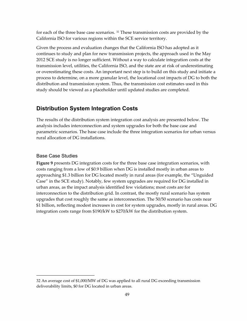
for each of the three base case scenarios. 32 These transmission costs are provided by the California ISO for various regions within the SCE service territory.

Given the process and evaluation changes that the California ISO has adopted as it continues to study and plan for new transmission projects, the approach used in the May 2012 SCE study is no longer sufficient. Without a way to calculate integration costs at the transmission level, utilities, the California ISO, and the state are at risk of underestimating or overestimating these costs. An important next step is to build on this study and initiate a process to determine, on a more granular level, the locational cost impacts of DG to both the distribution and transmission system. Thus, the transmission cost estimates used in this study should be viewed as a placeholder until updated studies are completed.

Distribution System Integration Costs

The results of the distribution system integration cost analysis are presented below. The analysis includes interconnection and system upgrades for both the base case and parametric scenarios. The base case include the three integration scenarios for urban versus rural allocation of DG installations.

Base Case Studies Figure 9 presents DG integration costs for the three base case integration scenarios, with costs ranging from a low of $0.9 billion when DG is installed mostly in urban areas to approaching $1.3 billion for DG located mostly in rural areas (for example, the “Unguided Case” in the SCE study). Notably, few system upgrades are required for DG installed in urban areas, as the impact analysis identified few violations; most costs are for interconnection to the distribution grid. In contrast, the mostly rural scenario has system upgrades that cost roughly the same as interconnection. The 50/50 scenario has costs near $1 billion, reflecting modest increases in cost for system upgrades, mostly in rural areas. DG integration costs range from $190/kW to $270/kW for the distribution system.

49

32 An average cost of $1,000/MW of DG was applied to all rural DG exceeding transmission deliverability limits, $0 for DG located in urban areas.

Figure 9: Integration Costs: Base Case Scenario

$‐

Total Cost ($ Millions

$200 $400 $600 $800 $1,000 $1,200 $1,400


)



Parametric Analysis Figure 10 presents DG integration costs under the assumption that all DG is installed in clusters at the end of the 13 distribution feeders. The impact analysis presented in prior sections resulted in findings that included frequent voltage violations and capacity overloads. Consistent with these findings, integration costs for system upgrades increase significantly—roughly twofold at the distribution level—compared to the base case. Total integration cost for scenarios presented in Figure 10 ranges from $260/kW to $420/kW for the distribution system.

Figure 10: Integration Costs: Clustered Distributed Generation (End of Feeder)

$‐

Total Cost ($ Millions

$500

$1,000

$1,500

$2,000

$2,500


)



50

Figure 11 presents the results of the high DG penetration scenario, where DG capacity is increased to 6,000 MW, or 1,200 MW above the base case. Results indicate the cost of distribution system upgrades increase modestly (about 25 percent) for the mostly urban DG scenarios: $0.9 billion versus $1.2 billion. However, the mostly rural DG case results in a 50 percent cost increase: $1.3 billion versus almost $2 billion.

Figure 11: Integration Costs: High Distributed Generation Penetration

$‐

$500

$1,000

$1,500

$2,000

$2,500





Cost Components Table 21 through Table 23 present costs by major component for the base case and parametric studies summarized in Figure 9 and Figure 10. The majority of costs are for line upgrades or replacement, as the cost of line regulators are far lower than line upgrades. Most of the upgraded lines include the replacement of smaller conductor, such as #6, #4, and #2 wire, with 336 aluminum conductor steel reinforced or equivalent. Two feeders in the 30 urban/70 rural clustered case included new feeders, as the amount of DG installed exceeded operational limits.

51

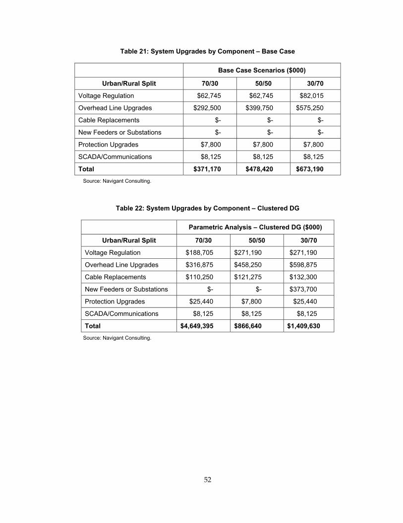
Table 21: System Upgrades by Component – Base Case

Base Case Scenarios ($000)

Urban/Rural Split 70/30 50/50 30/70

Voltage Regulation $62,745 $62,745 $82,015

Overhead Line Upgrades $292,500 $399,750 $575,250

Cable Replacements $- $- $-

New Feeders or Substations $- $- $-

Protection Upgrades $7,800 $7,800 $7,800

SCADA/Communications $8,125 $8,125 $8,125

Total $371,170 $478,420 $673,190 Source: Navigant Consulting.

Table 22: System Upgrades by Component – Clustered DG

Parametric Analysis – Clustered DG ($000)




Cable Replacements $110,250 $121,275 $132,300

New Feeders or Substations $- $- $373,700



Total $4,649,395 $866,640 $1,409,630 Source: Navigant Consulting.

52

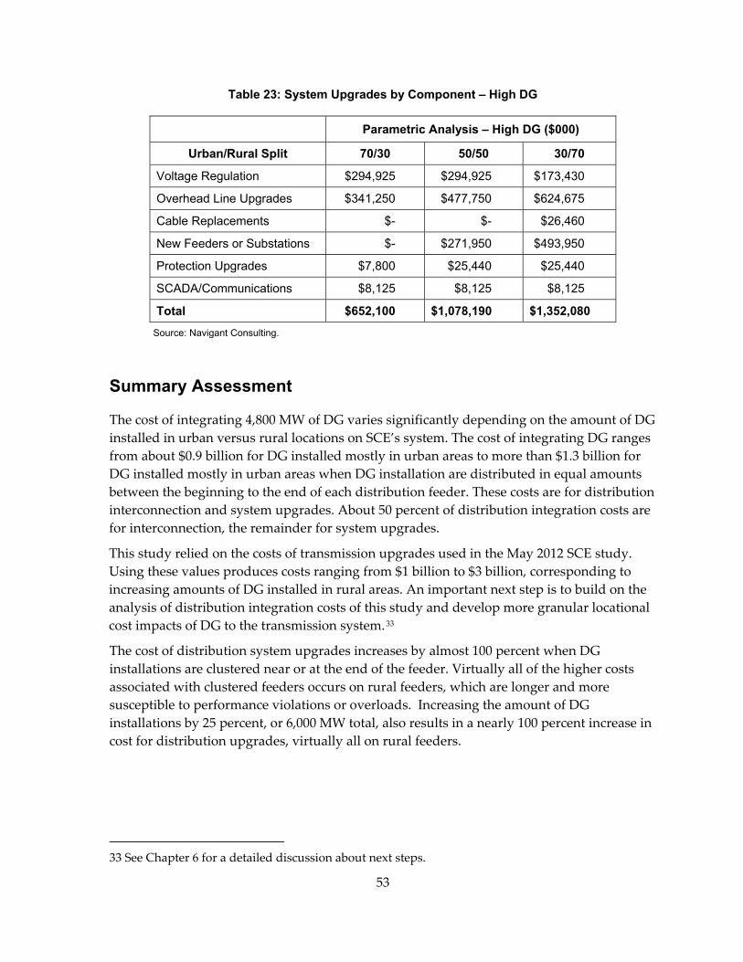
Table 23: System Upgrades by Component – High DG

Parametric Analysis – High DG ($000)




Cable Replacements $- $- $26,460

New Feeders or Substations $- $271,950 $493,950



Total $652,100 $1,078,190 $1,352,080 Source: Navigant Consulting.

Summary Assessment

The cost of integrating 4,800 MW of DG varies significantly depending on the amount of DG installed in urban versus rural locations on SCE’s system. The cost of integrating DG ranges from about $0.9 billion for DG installed mostly in urban areas to more than $1.3 billion for DG installed mostly in urban areas when DG installation are distributed in equal amounts between the beginning to the end of each distribution feeder. These costs are for distribution interconnection and system upgrades. About 50 percent of distribution integration costs are for interconnection, the remainder for system upgrades.

This study relied on the costs of transmission upgrades used in the May 2012 SCE study. Using these values produces costs ranging from $1 billion to $3 billion, corresponding to increasing amounts of DG installed in rural areas. An important next step is to build on the analysis of distribution integration costs of this study and develop more granular locational cost impacts of DG to the transmission system.33

The cost of distribution system upgrades increases by almost 100 percent when DG installations are clustered near or at the end of the feeder. Virtually all of the higher costs associated with clustered feeders occurs on rural feeders, which are longer and more susceptible to performance violations or overloads. Increasing the amount of DG installations by 25 percent, or 6,000 MW total, also results in a nearly 100 percent increase in cost for distribution upgrades, virtually all on rural feeders.

33 See Chapter 6 for a detailed discussion about next steps.

53

CHAPTER 5: Study Findings This section summarizes the study’s findings and conclusions. These include an assessment of the applicability of the analytical framework used in this study to other utilities and industry stakeholders, and how the approach can be used to identify DG impacts over a range of assumptions and scenarios. The Energy Commission and study participants are confident the approach presented in this report and the results obtained achieve this objective. Study results also provide guidance to policy makers regarding locational factors in terms of where DG should be actively promoted to help achieve renewable capacity goals and procurement objectives.

Analytical Framework

The methods and assumptions presented in this report provide an analytical framework that can be used by other California utilities. The framework, while rigorous, is not overly prescriptive with regard to the specific tools and assumptions that are required, but instead provide guidance to those seeking to employ methods that can be used to estimate DG integration costs with a reasonable level of confidence. It highlights the potential impacts that may result from integration of large amounts of DG and offers solutions to integration at least possible cost. It also illustrates how integration costs vary significantly as a function of location, both on an area or regional basis and when clustered on specific segments of a feeder. The framework also provides insight and lays the groundwork for evaluating and assessing advanced technologies, including smart systems and changes in industry guidelines and standards.

Distributed Generation Impacts and Integration Costs

Study results indicate integration impacts and the need for system upgrades are substantially greater in rural areas, where penetrations of distributed generation are high. Several of the longer, rural feeders experienced voltages above established thresholds as well as overloads on line sections equipped with smaller conductors. Few urban feeders experienced voltage violations, and none of the DG scenarios resulted in overloads on urban feeders.

Study results indicate the cost of interconnection and distribution system upgrades for 4,800 MW of DG on SCE’s distribution system could range from a low of $1 billion to a high of $2 billion, depending on DG size, location, and the amount of clustering of DG on distribution feeders. Although transmission costs were not derived for this study, estimates previously prepared by the California ISO and applied in SCE’s May 2012 study suggest transmission upgrades could add $1 billion to $3 billion, virtually all in rural areas where

54

transmission constraints are greatest. Study participants agree that transmission integration costs associated with increased penetrations of distribution connected generation should be studied sooner rather than later.

Smart Systems and Advanced Technologies

This study evaluates the impacts of DG integration and estimates the associated costs based on currently available technologies. However, the results of this and other studies, including ongoing investigations by the Energy Commission and other California agencies, suggest advanced technologies hold significant potential for reducing the impact and cost of integrating DG. Many of these technologies and approaches focus on automation and smart systems to manage the myriad size and type of DG technologies that likely will be seeking interconnection to the grid.

For lower DG penetration, the impact and cost of integrating DG are manageable for many electric grid operators. However, large amounts of DG potentially can overwhelm grid operators when conditions require adjustments to the grid configuration or status of DG units – automated systems may be essential to ensure grid reliability, operability, and safety. Although not specifically addressed in this effort, large amounts of DG also may impact bulk system operations. The same smart technologies employed to manage DG at the local level also may assist bulk system operators, particularly during major contingencies or abnormal conditions.

Conclusions

The Energy Commission study produced the following findings and conclusions associated with the integration of up to 12,000 MW of renewable DG in California:

• The cost of DG integration depends highly on locational factors for both the distribution and transmission systems.

• Generally, integration impacts and costs are lower when DG is installed in urban areas, where feeders are shorter and often equipped with larger conductor or cable along the entire length of the circuit.

• DG integration costs increase significantly as greater amounts of DG are clustered and installed near the end of distribution lines.

• Distribution planning and operational criteria and practices that ensure minimal impact to reliability and system operability can limit DG integration even on feeders where DG does not create loading or voltage violations.

• High‐penetration DG may require sophisticated communications and control systems to better manage DG impacts and reduce integration costs.

55

• Advances in smart system technology and changes in industry standards may provide an opportunity to enable greater amounts of DG at lower cost.

• Policies that guide or encourage DG in areas with fewer impacts would minimize grid integration costs; however, the lowest total cost solutions would need to factor in the procurement costs of the systems themselves.

• Results from this study, including variations in DG capacity by location, may provide guidance to the next DG deliverability study the California ISO will conduct in early 2014.

56

CHAPTER 6: Next Steps The Energy Commission considers this study as a first step toward the 2012 Integrated Energy Policy Report Update goals of identifying preferred areas for renewable distributed generation, and minimizing interconnection and integration costs and requirements.34 This study presents a framework for analyzing and quantifying the electricity system costs associated with increased penetration levels of DG. The costs provided by this study are location specific and demonstrate that a project’s financials greatly depend on its location, both from a regional perspective, and, on a more granular level. Location specific costs are important because they provide:

• More transparent price signals to developers so they can make better business decisions on where to locate projects.

• Useful information to utilities in making distribution system investment decisions.

• More granular information for the site and utilities to develop better planning assumptions with regard to where DG will be located.

This study’s scope was limited to looking at distribution system integration costs of renewable DG. It did not include a study of transmission‐level integration costs, nor did it include and evaluate other preferred resources, such as energy efficiency, demand response, or energy storage.35

The results of this study provide valuable insights, and the Energy Commission will build on this effort in the short term with two separate yet coordinated projects. First, the Energy Commission will partner with the California ISO and the utilities to develop a rigorous analysis of transmission system integration costs associated with increased penetrations of renewable DG. Second, the Energy Commission will launch a pilot project that, using the analytical framework of this study, will identify locations on the electricity system that, from a cost‐containment and value‐added perspective, are preferable for renewable DG and other preferred resources.

Future Transmission Integration Cost Analysis

One of key findings of this study is that DG integration costs depend highly on locational factors for both the distribution and transmission systems. This study focused on

57

34 California Energy Commission. 2012. 2012 Integrated Energy Policy Report Update. Publication Number: CEC‐100‐2012‐001‐CMF.

35 Energy storage was considered as a potential mitigation option, but because the study relies on existing technologies, it was determined not to be a cost‐effective option at this time.

distribution system integration costs and, due to time and funding constraints, relied on transmission integration costs that were used in the May 2012 SCE study. These transmission integration costs were derived from California ISO studies, performed specifically to determine dollar‐per‐MW estimates for transmission upgrades to accommodate DG. However, these costs are high‐level estimates based on transmission upgrade costs needed to mitigate congestion in transmission areas that were germane to the May 2012 SCE study. While they are an adequate placeholder for this study, it is critical that a more rigorous analysis of potential transmission integration costs is conducted that aligns distribution system constraints with transmission constraints. This is especially important since transmission integration costs make up a significant amount of total integration costs, particularly if DG development continues in the current unguided environment.

The Energy Commission has begun discussions with the California ISO to expand this study’s analytical framework to include an analysis of transmission integration costs. The expanded study will provide location specific transmission integration costs that can be mapped to distribution integration costs, yielding total system costs for higher DG penetration levels. The location‐specific total system costs will provide the state with much needed information to help identify preferred areas on the electricity system for DG development.

Additionally, the expanded study will explore how location‐specific total system costs can be used to develop better DG planning assumptions for the state’s Renewables Portfolio Standard portfolios. The California ISO relies on these assumptions for its DG deliverability study. The accuracy of the assumptions is important so that DG deliverability allocations are available either at transmission nodes that are not constrained, or at nodes that serve preferable locations for DG (deliverability potential can be a powerful incentive for guiding projects to preferred locations). The California ISO April 2013 DG deliverability study36 is limited by these assumptions given their overall lack of granularity, and the fact that they exclude several transmission nodes that are designated as having zero DG potential.37 Thus, there is uncertainty regarding the available transmission capacity at those transmission nodes. The next opportunity for specifying locations for DG to meet Renewables Portfolio Standard targets will be when the California ISO updates its DG deliverability study in early 2014.

58

36 http://www.caiso.com/Documents/2013DGDeliverabilityStudyResults.pdf.

37 For example, the current DG deliverability study examined only 56 out of 91 nodes in SCE service territory and identified 857 MW of DG deliverability potential, far short of the penetration levels needed to meet the 12,000 MW goal.

http://www.caiso.com/Documents/2013DGDeliverabilityStudyResults.pdf

State Planning Process Pilot

Both the Energy Commission study and the May 2012 SCE study concluded that policies that guide or encourage DG in areas with fewer electricity system impacts would help achieve state renewable goals at lower cost. The need for these policies is becoming increasingly important since current energy policy has DG becoming a larger portion of California’s generation portfolio. To date, there are almost 3,300 MW of renewable DG on‐line and another roughly 2,500 MW pending that may meet the Governor’s preferred definition of DG.38 Historically, DG penetration levels have grown slowly, with almost half of existing DG being interconnected between 1900 and 2005. Since then, the California Solar Initiative program has brought on‐line roughly 1,600 MW of customer‐side solar PV generation. To achieve a 12,000 MW DG penetration level will require interconnecting over the next seven years more than three‐and‐a‐half times the amount of DG that is currently operational.39 Additionally, recent legislation has lifted the net energy metering cap, opening the door for even more customer‐owned DG.40

To plan for and optimize the value of future DG resources, the Energy Commission, building on the findings of this study and the future expanded study discussed earlier, will launch a state planning process pilot project that identifies and evaluates areas on the utility electricity system best suited to accommodate DG. In defining the preferred areas, the initial focus will be on the utility system, as the ability to accommodate increased penetrations of DG is a significant barrier. The first phase of the planning pilot will look at the system from an available capacity, least‐cost‐to‐interconnect perspective. The second phase will look at optimizing the value of DG, as well as other preferred resources, such as energy efficiency, demand response, energy storage, and so forth.

Land‐use and environmental constraints must also be considered when identifying preferred locations for DG resources. The planning pilot will first identify areas on the electricity system; then it will evaluate the land‐use and environmental constraints within the footprint of those areas to determine where there are preferred land uses and minimal environmental impacts.41 By accounting for electricity system, land‐use, and environmental

59

38 Pending projects are not guaranteed to become operational. Furthermore, the numbers reflect projects that meet the resource type and size threshold of the definition. Whether they count toward the 12,000 MW goal depends how strictly the other criteria are applied.

39 The state has several procurement programs that incentivize development of a diverse set of DG resources, ranging from small rooftop residential PV to larger 20 MW ground‐mounted PV projects. For example, the Renewable Auction Mechanism program currently has a capacity cap of 1,299 MW, none of which are on‐line today, yet more than half of which are scheduled to be on‐line in the next few years.

40 Assembly Bill 327 (Perea, 2013).

41 Environmental impacts will vary greatly depending on DG project size, technology type, and location (for example, rooftop vs. ground‐mounted PV).

impacts, the planning pilot will provide further granularity on preferred locations by identifying where these metrics overlap. The results will yield a spectrum of locations that range from significant overlap to no overlap, with the goal of guiding projects to locations with the most overlap. The goal of the planning pilot is to develop a systemwide plan that identifies preferred locations where DG can minimize costs and provide value to the system, and where compatible land uses minimize environmental impacts.

60

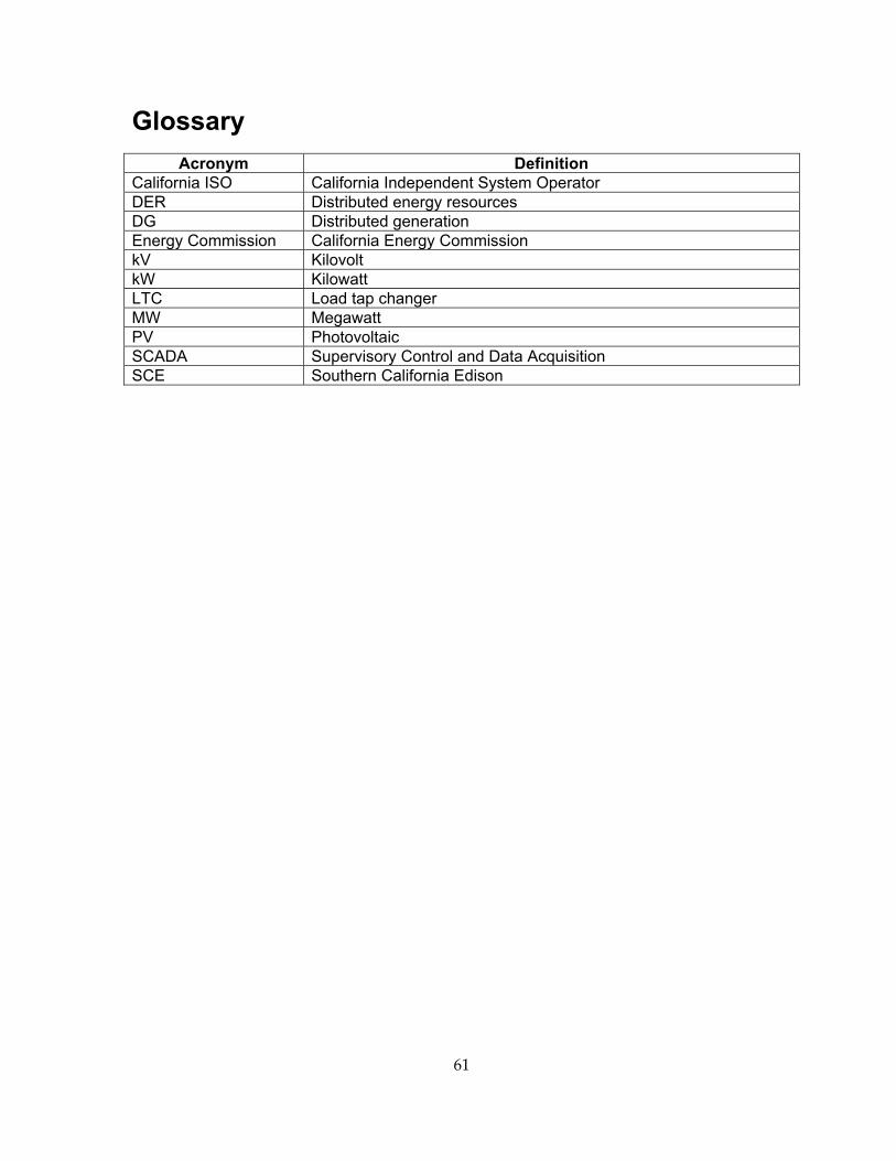
61

Glossary Acronym Definition

California ISO California Independent System Operator DER Distributed energy resources DG Distributed generation Energy Commission California Energy Commission kV Kilovolt kW Kilowatt LTC Load tap changer MW Megawatt PV Photovoltaic SCADA Supervisory Control and Data Acquisition SCE Southern California Edison

APPENDIX CYME/Milsoft Data Conversion Flowchart

CYME Input File

CYME

CYME Output File

SCE Feeder GIS Data- to- CYME Input File Auto Extraction

(contains Critical Infrastructure Information)

Milsoft Input File

Milsoft

Milsoft Output File

1SCE Feeder Characteristics

Excel Spreadsheet (contains ConfidentialInformation, no CII)

Navigant Selection Algorithm

Selected Feeders( qty ~10 - 20)

CYME - Milsoft Converter

12

11

10

9

8

7

6

5

4

3

2

Send to Navigant

Send to Navigant

13 CYME - to- Milsoft

Navigant Task

Conversion Validation

Cleanup, V alidation, & Removal of CII Geospatial Data

SCE Task


A‐1

Feeder Diagrams

All feeder diagrams are provided by Navigant Consulting.

Feeder No. 1

A‐2

Feeder No. 2

A‐3

Feeder No. 3

Feeder No. 4

A‐4

Feeder No. 5

Feeder No. 6

A‐5

Feeder No. 7

Feeder No. 8

A‐6

Feeder No. 9

Feeder No. 10

A‐7

Feeder No. 11

Feeder No. 12

A‐8

A‐9

Feeder No. 13