Dissolved Oxygen Fluctuation Regimes in Streams of the Western Corn Belt Plains Ecoregion

Report No. 130 of the Kansas Biological Survey

November 2005

By the Central Plains Center for BioAssessment

Donald G. Huggins Jeff Anderson

University of Kansas Takeru Higuchi Building

2101 Constant Avenue, Room 35 Lawrence, KS 66047-3759

www.cpcb.ku.edu

Prepared in fulfillment of USEPA Award X7-99790401

1

INTRODUCTION

As we consume more of our natural resources, it becomes increasingly apparent that

we must do everything possible to insure that these resources will still be viable in the future.

In building upon the Clean Water Act of 1972, the U.S. government developed and issued the

Clean Water Action Plan (CWAP) in 1998. The CWAP was designed to protect public

health from polluted waters, improve the control of polluted land runoff, and promote the

protection of water quality on a watershed basis. In response to the CWAP, the U.S.

Environmental Protection Agency (USEPA) developed the National Strategy for the

Development of Regional Nutrient Criteria (NSDNC). The NSDNC outlines a framework

for developing water body-specific, technical guidance used to assess nutrient status and

develop regional nutrient criteria (USEPA 1998). Within this framework, the USEPA

identified several areas in which to focus research. These areas include grey literature on

nutrient data, studies on instream chlorophyll levels, and diel dissolved oxygen fluctuation

related to instream nutrient concentrations. The USEPA formed Regional Technical

Assistance Groups (RTAG) to address these topics throughout the country. The Central

Plains Center for BioAssessment (CPCB) at the Kansas Biological Survey is a member of the

USEPA Region 7 RTAG and is working with other members from states and tribes in Iowa,

Kansas, Missouri, and Nebraska on various aspects of the research topics. CPCB has led this

study that attempts to address several of the identified research needs and focuses on how

instream nutrient concentrations (and other factors) may affect diel dissolved oxygen

fluctuation and impact primary production.

The established and quantifiable relationships commonly observed in lakes and

reservoirs, for example total phosphorus and hypolimnetic dissolved oxygen deficit (Welch

2

1992), do not exist for streams and rivers (Dodds et al. 1998). However, it is believed that

these types of relationships could be developed for streams and rivers (EPA 2000).

Incomplete and “snap shot” measures of temporal and diel dissolved oxygen (DO) patterns is

one reason that statistical analysis of instream variables and dissolved oxygen yield poor

relationships (Uehlinger and Naegeli 1998). Dissolved oxygen levels fluctuate throughout

the day and nighttime periods (i.e., diel flux) by as much as 10 mg/L. Many past projects

that attempted to draw relationships among dissolved oxygen and other instream variables

have used a single dissolved oxygen measure for each stream that may have been taken at

any point on the diel oxygen cycle and during any time of the year. The CPCB has compiled

a database of over 25,000 records from streams in EPA Region 7 from a number of sources

(i.e. U.S. Army Corps of Engineers, Iowa Department of Natural Resources, Kansas

Department of Health and Environment, Missouri Department of Natural Resources,

Nebraska Department of Environmental Quality, USEPA, U.S. Geological Survey) in which

measures for dissolved oxygen are reported as a single value for each site. Because oxygen

levels exhibit patterns that reflect the results of exogenous and endogenous factors operating

at differing time scales that cannot be discerned by single point-in-time measures, it is little

wonder that few if any relationships have been quantified. By examining continuous

measurements of dissolved oxygen, it is hypothesized that the relationships between the

watershed, water chemistry, nutrients, stream biota and dissolved oxygen will become more

apparent. This study focuses on identifying and defining potential causal relationships

among stream nutrient concentration, dissolved oxygen levels and daily oxygen flux during

summer growing periods.

3

Nutrients provide vital sustenance for both terrestrial and aquatic plants. In aquatic

ecosystems, excessive concentrations of nutrients can lead to declines in water quality as well

as undesirable changes in the ecology of water bodies. Evidence from a wide array of studies

showed that lotic systems are sensitive to anthropogenic inputs of nitrogen and phosphorus,

the two macro-nutrients essential for plant growth (Smith et al. 1999).

Cultural eutrophication is a leading cause of impairment in U.S. surface waters

(USEPA 1996). Eutrophication is often a normal part of the natural aging process of a lentic

body of waters. Cultural eutrophication occurs when nutrient loads and concentrations

increase due to anthropogenic activities and factors often associated with the watershed or

airshed of a waterbody. Nitrogen and phosphorus are the primary nutrients limiting

eutrophication in nearly all freshwater ecosystems except for some waterbodies in which

nitrogen is the limiting factor in aquatic plant production (USEPA 2000).

Nutrient impaired waters can cause problems ranging from recreational annoyances,

to serious public health concerns, to adverse effects on the ecology of the aquatic ecosystem

(Dodds and Welch 2000). High levels of algae and macrophytes can develop quickly in

response to excessive nutrient inputs. Eutrophication can restrict water use for fisheries and

recreation (Sharpley et al. 2000). Although autotrophic biomass is important in many

streams as a food source for organisms (Lamberti 1996), algal blooms can produce toxins

such as microcystin and trihalomethanes (THMs) that affect livestock and human health

(Palmstrom et al. 1988, Kotak et al. 1994, USEPA 1998, USEPA 2000). Stimulated by

nutrients, harmful algal blooms such as brown tides and Pfiesteria have lead to major fish

kills in costal areas (Palmstrom et al. 1988, Kotak et al. 1994). High concentrations of

ammonia are toxic to fish and nutrients like nitrate can have direct detrimental effects when

4

ingested by humans (Matson et al. 1997). Increased nutrient enrichment can directly and

indirectly affect the ecology of the aquatic ecosystem by degrading water quality, altering

instream habitat and changing primary producer communities and production. High algal

and macrophyte biomass may be associated with severe swings in dissolved oxygen (USEPA

1998, Sharpley et al. 2000). Low dissolved oxygen concentrations can increase the

availability of toxic substances (e.g. ammonia), thereby reducing the amount of quality

habitat for aquatic organisms.

Aside from changes in the structure and function of aquatic ecosystems, nutrient

impairment can affect the quality of drinking water resulting in increased treatment expenses

(USEPA 2000). Increases in algae and macrophytes from nutrient impairments often leads to

clogged intakes for water treatment plants. The increased biomass in water sources requires

additional chemicals and longer settling times to attain acceptable water quality.

Several factors regulate the instream concentration of dissolved oxygen and these are

compounded by eutrophication caused by macronutrients nitrogen and phosphorus. Drainage

accrual, diffusion of oxygen across the air/water interface, and stream biota control the level

of instream oxygen (Odum 1956).

The input of oxygen rich or oxygen poor waters by drainage accrual results in

changes to dissolved oxygen concentrations. Drainage accrual is attributed to the upwelling

of groundwater into the stream flow (Uehlinger and Naegeli 1998), runoff from the

surrounding watershed, inputs from agricultural drainage tiles, or through municipal

wastewater discharges. Since these waters are typically low in dissolved oxygen

concentrations, their introduction lowers the concentration of dissolved oxygen in the stream

(Naiman and Bilby 1998). However, the addition of waters by groundwater or vadose water

5

accrual may stimulate the uptake of dissolved oxygen through community respiration and

thus enhance stream community respiration.

Diffusion of oxygen across the air-water interface tends to moderate changes in

dissolved oxygen concentrations in streams. For streams that have a high surface area to

volume ratio, like the small, relatively shallow streams examined in this study, diffusion

becomes a major component in the regulation of instream oxygen concentrations. As

dissolved oxygen levels depart from saturation levels, oxygen will diffuse into or out of the

stream in order to maintain an oxygen concentration near saturation (Wilcock et al. 1995).

Changes in dissolved oxygen concentrations due to photosynthetic production or respiration

will only be detected when these biotic changes in oxygen concentration exceed the rate of

change due to diffusion.

The third component affecting dissolved oxygen concentrations in streams is stream

biota. The metabolic activity of stream organisms controls the level of productivity in the

stream. Viable macrophyte and algae populations produce oxygen as a byproduct of

photosynthesis thus increasing the concentration of dissolved oxygen while whole system

respiration demands use oxygen. The respiratory activity of fish, benthic invertebrates and

bacteria continuously utilizes dissolved oxygen while plant respiration is limited to dark

photoperiods. Bacterial decomposition of autochthonous organic mater from decaying

primary producers and stream organisms along with the decomposition of allochthonous

inputs of organic matter consume dissolved oxygen. Biological modification of the oxygen

regime leads to a more productive environment and greater fluctuations in concentrations

during the day (Horne and Goldman 1994). This production of oxygen during the day and

6

continuous consumption of oxygen throughout the day/night periods drives the fluctuating

diel cycle of dissolved oxygen.

In situations where drainage accrual is negligible and rates of diffusion are known or

can be estimated, the relationship between changes in dissolved oxygen concentrations and

the metabolic activity of stream biota can be used to calculate values of production and

respiration. Odum (1956) presented the diurnal oxygen curve method, which estimates daily

gross primary production and community respiration from changes in measured stream

dissolved oxygen concentrations over time. Since this method measures the entire stream

community it should provide more representative results than chamber measurements that

neglect many of the dynamic factors that influence whole stream metabolism (Marzolf et al.

1994). When reaeration coefficients can be accurately estimated, Odum’s diurnal curve

method provides an accurate measure of gross primary productivity (Bott et al. 1978).

Primary productivity patterns in lotic ecosystems have been shown to respond to

downstream changes in ecological processes and stream morphology (Naiman and Bilby

1998). Vannote and co-researchers describe these trends in stream function in the river

continuum theory introduced in 1980 (Vannote et al. 1980). This theory views river systems

as a continuum of geophysical and hydrological changes with an associated gradient of biotic

communities in which structure and function changes. Community metabolism is a main part

of the theory (Fleituch 1999). The theory proposes that small headwater streams are

generally strongly influenced by riparian vegetation, which reduces primary production

through shading and inputs large amounts of organic detritus. This results in gross primary

production to respiration ratios (P/R) of less than one. Minshall (1978) points out that this

concept is modeled on natural, undisturbed stream ecosystems. The longitudinal profile of

7

productivity in agriculturally dominated prairie streams, like those selected in this study, has

been shown to deviate from the current theory (Wiley et al. 1990). Anthropogenic

disturbances like those found in the agriculturally dominated watersheds of Western Corn

Belt Plains streams could increase P/R ratios.

The streams in this study are located in the Western Corn Belt Plains (WCBP) of the

U.S. and were selected because of their agriculturally dominated watersheds, relatively open

canopied stream channels and high nutrient concentrations. Nutrient inputs from fertilizers

and alteration of riparian vegetation by farming, grazing, or channelization may have a

significant impact on the metabolic activities of the stream biota. The sparse canopy

structure of many of the riparian corridors in the WCBP provides little shading. The high

light intensities, combined with high nutrient levels are expected to result in high rates of

production that cause large fluctuations in dissolved oxygen concentrations and potentially

low DO levels during all or parts of the diel period.

Study Objectives

The overall goal of this study was to quantify DO values and DO flux in small

streams under normal or low flow conditions associated with late summer and investigate

possible causal relationships among DO and a number of stream and watershed factors. This

study focused on wadeable streams of the Western Corn Belt Plains of the Central Plains

region because their watershed are dominated by cultivated cropland and thus receive high

inputs of nutrients. It was anticipated that these streams were highly productive and

therefore susceptible to large diel swings in oxygen concentrations and low DO

concentrations. It was hypothesized that relationships among DO and stream nutrients and

8

other variables could be quantified by continuously monitoring instream dissolved oxygen

concentrations through daily or weekly time periods and comparing these values with grab

sample chemistry.

The objectives of this study were:

1. Quantify the diel fluctuations of dissolved oxygen in wadeable streams within the

Western Corn Belt Plains.

2. Quantify stream production and respiration in wadeable streams within the

Western Corn Belt Plains.

3. Examine the possible relationships among dissolved oxygen, stream productivity,

and instream and watershed factors.

STUDY DESIGN AND METHODS

Ecoregional Approach and Study Sites

The Western Corn Belt Plains (WCBP) of the central U.S. (Figure 1) ecoregion was

selected as the area of study because lotic ecosystems in this region are typically low gradient

streams with fine (e.g. sand, silt) bottom substrates. In mid- to late summer water

temperatures often exceed twenty-eight degrees Celsius and flows are generally at or near

yearly low flow averages. In addition, high inputs of nutrients are the result of the rather

intense agricultural land use associated with nearly all of the ecoregion. Streams within the

Western Corn Belt Plains (WCBP) were thought to be highly susceptible to dissolved oxygen

(DO) depletion as a potential result of the cumulative effects of the factors mentioned above.

These streams reflect the nature of the landscape they drain. This regional approach reduced

the effects among stream sites of spatial differences (i.e. soils, geology, land use practices,

9

etc.) that could bias measurements if regional boundaries were ignored. Omernik’s (1987)

ecoregion classification scheme was employed because it was designed to aid in

understanding the regional patterns of aquatic and terrestrial resources and their attainable

quality. This ecoregion framework was based on climate, mineral availability, vegetation,

and physiographic factors.

The WCBP ecoregion forms part of the landscape in the states of Iowa, Kansas,

Minnesota, Missouri, and Nebraska, with the majority of the region occurring within Iowa.

With over ninety percent of the Western Corn Belt Plains used for agriculture, the WCBP is

well known for its highly productive cropland (Chapman et al. 2001). Crops such as alfalfa,

corn, sorghum, soybeans, and wheat dominate this ecoregion that was once covered by tall

grass prairies. Topography varies from level alluvial plains to gently rolling glaciated till to

hilly loess plains. Warm, fertile, moist soils cover the region and on average receive fifty-

eight to eighty-nine centimeters of precipitation annually, mainly during the harvest season.

The high concentration of cropland and livestock creates major environmental concern with

regard to surface and groundwater contamination.

During the summers of 1999 and 2000, thirty-six streams in the WCBP ecoregion

were monitored and analyzed to address basic questions regarding DO flux and

concentrations, and possible relationships with other abiotic and biotic factors (Figure 1).

Sixteen of these streams and watersheds had been previously studied for two and a half-years

as part of a grant funded by the USEPA and so were selected for study in 1999. In 2000,

twenty additional streams were added to the study to provide better spatial coverage of the

ecoregion and to examine stream systems with a history of either limited or high nutrient

concentrations. Watershed drainage areas ranged from approximately 3,000 to 55,000

10

hectares. Variation between stream sizes was controlled by limiting study streams to fourth

and fifth order streams or smaller. Also, limiting the study to low order streams provided

Figure 1. Map of the streams sampled during the summer of 1999 and 2000. The dark tan- colored region is the Western Corn Belt Plains ecoregion that occurs mainly in Iowa. less complex watersheds that both have a higher potential for isolating the variables of

interest and represent ecosystems with maximum terrestrial/aquatic interface. Unlike higher

order streams that are affected by the many separate watersheds that make up their drainage

basins, low order streams are more affected by their immediately surrounding watersheds

because of the high land/water interface. Additionally, because large watersheds are

typically aggregates of smaller watersheds, identifying and resolving relationships among

variables within the more manageable smaller watersheds directly contributes to large

watershed management. This allowed for the exploration of water quality interactions across

11

spatial scales by examining the connection between the composition of the watershed and

water quality measurements made at the stream site. Furthermore, the low order streams and

their smaller watersheds are less costly and easier to study.

Seasonal Variation

Many of the physical, biological and chemical characteristics of lotic systems vary

temporally as they respond to seasonal changes in climate and landscape conditions. Much

of the temporal variation in the data was reduced by focusing the monitoring effort into brief

sampling episodes with the late summer period that is characterized by high stream

temperatures and minimal flows. It is hypothesized that the stream ecosystem experiences

high levels of anthropogenic stress during the low flow period of late summer. Two

predominate climate variables that can have critical effects on the stream ecosystem are

naturally limited precipitation and high temperatures. Decreases in precipitation contribute

to the reduction in stream flows from the normal baseflow regime to lower, more stable flow

conditions. Thus during low flow periods, stream flow tends to be stable and with reduced

stream power, instream habitat differences are often more pronounced with pools that have

near zero velocity and reservoir-like conditions, and the heating capacity of the stream is

elevated. High temperatures of late summer increase stream temperatures, facilitating high

algal productivity and metabolic rates, while stable stream conditions promote accumulation

of algae biomass (USEPA 2000). Algal populations thrive under these conditions, which can

lead to increases in the frequency, duration and extent of algal blooms and “die offs.” Large

increases in algal production and biomass contribute to both high and low levels of DO and

large diel fluctuations of instream DO concentrations as a result of gross production and

12

community respiration demands. Collectively these factors result in DO-induced ecosystem

stress and negative impacts to stream biota.

Daily Variation

Rainfall events occurring in the study stream watersheds during the study period may

have directly and/or indirectly affected short-term primary production, DO, and water

temperature regimes for these streams. Rainfall events of sufficient intensity and duration

can result in near immediate surface runoff and increased stream flows. These elevated

flows from runoff can result in increased turbidity, increased or decreased water

temperatures, and increased nutrients and/or oxygen-demanding substances. In addition,

runoff conditions can result in the physical scouring of periphyton. Associated increases in

cloud cover may also significantly reduce in solar irradiation and air and water temperatures.

Moderate to large changes in any one of these factors or conditions as a result of single or

multiple events can affect DO values, fluctuations in these values, and/or primary production

of these streams during a sampling period. Similarly, larger scale temporal (e.g., shorter day

length, cooler temperatures) and spatial (e.g., reduced riparian shading, cultivation) changes

affect both the rate and patterns of primary production and community respiration. In order

to account for the potential effects of short-term climate phenomena (e.g., rainfall, air

temperature, and solar irradiation) on stream measurements and estimated stream processes

during the sampling period, daily precipitation data was obtained from the National Climatic

Data Center (NCDC). The NCDC’s Daily Surface Data series provided by state the station

names and identification numbers along with daily precipitation values (measured to

hundredths on an inch) and location coordinates. Each state’s monitoring network comprised

300 to 450 weather stations that record precipitation.

13

To associate DO study sites with local precipitation stations, both the NCDC

precipitation stations and DO stream study sites were mapped and displayed in ArcView. A

24-kilometer radius circle centered on each study site was delineated to help identify

precipitation stations recording rainfalls that may have influenced the site’s stream flow or

climate conditions. Precipitation data within each 24-kilometer circle were then examined to

quantify precipitation conditions just prior to and during the sampling time for each selected

site. Any day (24-hour period) with precipitation over one third of an inch (10.8 cm) was

flagged for possible significance as a potential indicator of surface runoff within the

watershed draining to the site. Since the precipitation stations are not located exactly where

the study sites are, it can be debated as to whether or not any rain actually fell at the study

site or in the watershed. Thus, each recorded precipitation event (i.e. single or multiple days)

was compared with graphs of the raw DO and water temperature data.

The corresponding segments of the raw DO and water temperature graphs were

inspected for anomalies that might be attributed to a change in local weather and/or stream

flows resulting from surface runoff. It was hypothesized that if the precipitation event

resulted in significant changes then it would cause a visual anomaly in the water temperature

or DO graphs. These visual responses most likely would be observed as changes in the

shapes and values of individual diel curves that correspond to the precipitation period when

compared to the complete series of diel curves generated during the study period. When a

graphed DO or temperature anomaly (i.e. stream disturbance) and precipitation event of one

third of an inch or greater coincided, it was assumed that a significant precipitation event was

responsible for the noted changes in the DO and temperature graphs. In this case, the

corresponding DO and temperature data were not used to calculate the average DO flux and

14

production for normal (non-runoff) days. Furthermore, if graphed anomalies did not coincide

exactly with the precipitation event, but appeared to be somewhat advanced or delayed (12-

36 hours), it was assumed that the precipitation event was still responsible for the noted

anomalies and that direct time correlations were affected by the spatial position of the

reporting precipitation stations relative to the study site and/or time-related flow responses.

In these cases, the offset associated diel data were grouped with data affected by climate and

removed from the analyses of non-runoff data.

Occasionally, a precipitation event of one third of an inch or less of precipitation was

recorded but no corresponding discernable disturbances or anomalies in the graphs were

observed. In these few instances, it was concluded that the precipitation event did not cause

sufficient changes in local weather (e.g. cloud cover, air temperature change) or stream flow

to alter the DO or temperature patterns in the monitored stream segment. Thus, the DO flux

data in these cases were retained and used to estimate values for non-runoff periods. In

practice, it was found that the majority of precipitation events over one-half inch were

correlated to a disturbance in the raw data graphs.

Procedures and Study Variables Site Selection

Stream sampling events were targeted for the low flow, high temperature period of

late summer starting in 1999 and continuing through the late summer periods of 2000 and

2001. Sampling sites were located between 50 and 100 meters upstream of bridge crossings

except where stream access was limited, in which case best professional judgment was used

to choose the site. In an effort to reduce instream variation associated with stream

15

macrohabitats (e.g. velocity, depth, mixing), only runs were sampled. A single Aqua 2002

Dissolved Oxygen and Temperature Data Logger® (BioDevices Corp, of Ames, Iowa, 1999)

was deployed at each stream site to continuously monitor stream temperature and DO. At the

sampling site, steel fencing T-posts were positioned in the thalweg of a run and driven into

the streambed at a downstream angle. Data Loggers were then attached to the backside of

the fence posts with cable ties and padlocked to the posts to reduce thief and vandalism. The

sensor heads of the Data Loggers were positioned approximately four centimeters above the

bottom substrate. The Data Loggers were positioned close to the streambed in the thalweg so

that under reduced flow conditions they would remain submerged and functioning properly.

Following the procedures outlined in the Data Logger manual, the Data Loggers were

calibrated as a group under the same aeration conditions prior to and during the study period.

Measurements of dissolved oxygen and water temperature were taken at ten minutes intervals

throughout the two-week long deployment period. At the end of this period, the logger was

removed and the data was downloaded to a laptop computer.

Water Chemistry

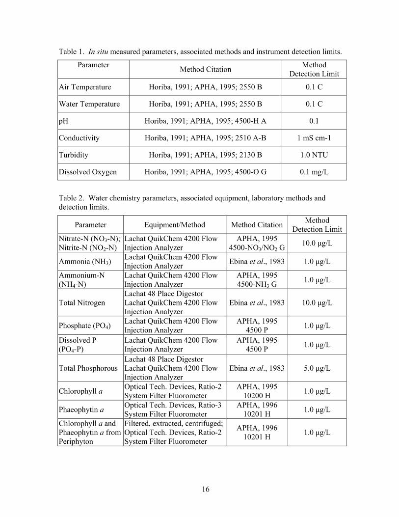
At the start and end of each logger deployment period a series of in situ water quality

measurements (Table 1) were taken using a Horiba U-10 Water Checker U10. In addition, a

water sample was collected in a one liter amber glass jar during installation and during

removal of the Data Logger. Samples were stored in coolers and packed with ice until

delivered within four days to the laboratory for analysis using standard analytical procedures

(Table 2). In addition to the parameters analyzed for in Table 2, several variables were

16

Table 1. In situ measured parameters, associated methods and instrument detection limits.

Parameter Method Citation Method Detection Limit

Air Temperature Horiba, 1991; APHA, 1995; 2550 B 0.1 C

Water Temperature Horiba, 1991; APHA, 1995; 2550 B 0.1 C

pH Horiba, 1991; APHA, 1995; 4500-H A 0.1

Conductivity Horiba, 1991; APHA, 1995; 2510 A-B 1 mS cm-1

Turbidity Horiba, 1991; APHA, 1995; 2130 B 1.0 NTU

Dissolved Oxygen Horiba, 1991; APHA, 1995; 4500-O G 0.1 mg/L

Table 2. Water chemistry parameters, associated equipment, laboratory methods and detection limits.

Parameter Equipment/Method Method Citation Method Detection Limit

Nitrate-N (NO3-N); Nitrite-N (NO2-N)

Lachat QuikChem 4200 Flow Injection Analyzer

APHA, 1995 4500-NO3/NO2 G 10.0 µg/L

Ammonia (NH3) Lachat QuikChem 4200 Flow Injection Analyzer Ebina et al., 1983 1.0 µg/L

Ammonium-N (NH4-N)

Lachat QuikChem 4200 Flow Injection Analyzer

APHA, 1995 4500-NH3 G 1.0 µg/L

Total Nitrogen Lachat 48 Place Digestor Lachat QuikChem 4200 Flow Injection Analyzer

Ebina et al., 1983 10.0 µg/L

Phosphate (PO4) Lachat QuikChem 4200 Flow Injection Analyzer

APHA, 1995 4500 P 1.0 µg/L

Dissolved P (PO4-P)

Lachat QuikChem 4200 Flow Injection Analyzer

APHA, 1995 4500 P 1.0 µg/L

Total Phosphorous Lachat 48 Place Digestor Lachat QuikChem 4200 Flow Injection Analyzer

Ebina et al., 1983 5.0 µg/L

Chlorophyll a Optical Tech. Devices, Ratio-2 System Filter Fluorometer

APHA, 1995 10200 H 1.0 µg/L

Phaeophytin a Optical Tech. Devices, Ratio-3 System Filter Fluorometer

APHA, 1996 10201 H 1.0 µg/L

Chlorophyll a and Phaeophytin a from Periphyton

Filtered, extracted, centrifuged; Optical Tech. Devices, Ratio-2 System Filter Fluorometer

APHA, 1996 10201 H 1.0 µg/L

17

calculated from these data. Organic nitrogen was taken as total Kjeldahl nitrogen minus

ammonia while organic phosphorus was calculated as total phosphorus minus dissolved

phosphate. Nitrogen to phosphorus ratios were calculated using total nitrogen and total

phosphorus. Also at the start and end of the logger deployment period, three to five

periphyton samples were collected using the techniques outlined in Bouchard and Anderson

(2001, unpublished manuscript) and returned to the laboratory for chlorophyll and

phaeophytin analysis.

Velocity and Depth

At the start and end of each logger deployment period velocity and depth were

measured along a series of five transects located at 20 to 30 meter intervals upstream from

the logger at each study site. Measurements were made using a Swoffer Model 2100 Current

Velocity Meter as outlined in the Swoffer manual. Eight or more measures were taken across

each transect. Weighted averages for velocity and depth values were calculated for each

transect and then averaged across the entire stream segment to produce a single estimate of

velocity and depth for the stream segment upstream of the logger site.

This approach was thought to provide better representation of stream flow characteristics that

could effect the reaeration potential at the logger (sampling) site than could a single set of

measurements from 1 transect at the logger site. Stream discharge was calculated from

cross-sectional transect data (i.e. velocity and depth measurements) using the methods of

Maidment (1993).

Landuse/Landcover

Land use/land cover (LULC) data were compiled using geographic information

systems and were derived from the EPA’s Multi-Resolution Land Characteristics (MRLC)

18

dataset. The MRLC project was established to provide multi-resolution land cover data of

the conterminous United States from local to regional scales (Bara 1994). This LULC

dataset was chosen because MRLC data was available in a seamless coverage for the entire

study region and utilized a high number of LULC classes that provided a detailed assessment

of the region.

Watersheds were defined as all of the land that drains to the sampling site. Based on

the coordinates of the Data Logger at each site, the watersheds were mapped using ESRI’s

ArcView 3.2 software and displayed in ArcView with the River Reach 1 stream coverage for

the WCBP and 1:24,000 scale USGS digital raster graphics (DRG) topographic maps of

drainage areas. Utilizing the contour lines on the DRGs, the watersheds were delineated by

digitizing the ridgeline that defined the area of land that drains surface water to the sampling

site. The stream coverage aided in defining the extent of the watershed, while the sampling

coordinates defined the lowest point of the watershed. Once the watersheds were delineated,

they were re-projected as necessary to match the map projection of the MRLC image and

overlaid on the MRLC image. Using ArcView’s Spatial Analyst extension package, the area

(m²) of each LULC class occurring within each watershed was computed and divided by the

total area of the watershed to determine the percent composition for each class. This was

done so that LULC comparisons could be made among watersheds using standardized

variables.

Estimates of gross primary production and community respiration were calculated

from diel oxygen and temperature data curves following the widely used and generally

accepted method of Odum (1956). To estimate production, a computer program was created

19

from Odum’s methods in Microsoft Excel. This productivity calculator is explained in detail

in the following section.

The DO and temperature data was graphed over time to check the flux patterns for

anomalies or irregularities (see Daily Variation section) that might have been due to

precipitation, siltation, or a malfunction of the logger itself. If data anomalies were

identified, those twenty-four hour cycles containing anomalies were removed from the

datasets. Next, the DO and temperature data were prepared for graphical and statistical

analysis. First, percent saturation values were calculated from the DO and temperature data

to allow standard comparisons to be made between watersheds (APHA, 1998). Next, a series

of statistical variables were calculated using both the raw DO and the percent saturation DO

values. The calculated variables included daily average, median, mode, standard deviation,

maximum, minimum, and the difference between the maximum and minimum values.

Averages for the sampling period (five to fourteen days) were calculated for each sampling

site from the daily averages.

Instream Productivity

Odum (1956) productivity methods were incorporated into the Productivity

Calculator developed for this study. The rate of change of dissolved oxygen (Q) is affected

by four main factors that include the rate of gross primary production (P), the rate of

community respiration (R), the rate of oxygen diffusion (D), and the rate of drainage accrual

(A) (Odum 1956). The majority of studies conducted on estimates of production derived

from diel oxygen data follow the method set forth by Odum (1956).

20

The rate of change of dissolved oxygen can be determined by subtracting both the

rate of community respiration (R) and oxygen diffusion (D) from the rate of gross primary

production (P) plus the rate of drainage accrual (A) as shown in Equation 1.

Q = P – R – D + A (1)

The fluctuation of dissolved oxygen levels in the stream due to drainage accrual is assumed

negligible relative to the other factors, but as a precaution, monitoring days in which

dissolved oxygen readings could have been impacted by rainfall should be removed from the

study dataset. This simplifies Equation 1 to Equation 2, the basic equation used to compute

gross production.

Q = P – R – D (2)

There are several other factors that also affect the concentration of dissolved oxygen

in streams and must be examined in order to provide more accurate estimates of production.

These factors are reaeration, temperature, salinity, and pressure.

Reaeration of streams is caused by two factors: entrainment of oxygen due to

turbulent flow and the replacement of oxygen due to a deficit from saturation caused by the

combustion of organic matter. Reaeration was originally defined in the Streeter-Phelps

(1925) equation as the reoxygenation (k2) of streams. Today it is largely understood that the

effects of the hydraulic properties of water (i.e. turbulent flow) are expressed as the

coefficient of reaeration, k2 (Langbein and Durum 1967).

The single most important factor regulating the concentration of dissolved oxygen in

water is temperature (Horne and Goldman 1994). The concentration of oxygen in water is

inversely proportionally to water temperature. Cold waters contain higher oxygen

concentrations than the same volume of warm water at a given pressure.

21

Changes in barometric pressure alter the concentration of dissolved oxygen, since all

gases are more soluble at higher pressures. This same principle is directly applicable to

increases in altitude. In these instances where pressures are less due to increased altitude,

concentrations of dissolved oxygen are reduced.

Salinity has a minor effect on dissolved oxygen concentrations in fresh waters when

compared to the other constituents. Increases in dissolved salts reduce the intermolecular

space with in the water molecules available to oxygen. Salinities must be high for increases

in salt concentrations to effect dissolved oxygen concentrations. Conductivity was used in

the calculator as an alternative input variable to salinity, because of its relationship to salinity

and greater commonality of measure.

An understanding the influencing factors leads back to Equation 2. The first

component of Equation 2 that needs to be solved for is D, the rate of oxygen diffusion. There

are several aspects that affect the rate of oxygen diffusion (D). The reaeration coefficient

k2,20, in units of 1/day, is one of the first variables to define. Several authors, Owens et al.

(1964) and O’Connor and Dobbins (1958) among others, have developed simple predictive

equations for the estimation of k2,20. Wilcock (1982) has provided an overview of some of

the most widely used reaeration equations and the stream conditions for which the equations

are most viable. The vast majority of these equations are of the form:

cb zaUk ⋅=20,2 (3)

Where U is the mean stream velocity (m/s), z is the mean stream depth (m), and a, b, and c

are constants. Once k2,20 is computed, it must be corrected for temperature. This conversion

is accomplished using the Elmore and West (1961) equation.

22

2020,2,2 024.1 −⋅= CT

T kk (4)

A new temperature corrected reaeration coefficient, k2,T, must be calculated for each recorded

measurement of dissolved oxygen since the temperature is also recorded at the same time and

does fluctuate throughout the day and night.

After calculating k2,T, the concentration of dissolved oxygen at saturation for each

recorded temperature must be calculated. During these computations corrections for salinity

and pressure will be addressed. In order to calculate the dissolved oxygen concentration in

mg/L at the standard pressure of one atmosphere, pC , all temperature values are converted

from Celsius to Kelvin, Equation 5.

15273.TT CK += (5)

The temperature in Kelvin, KT , is used to calculate the dissolved oxygen concentration in

mg/L at the standard pressure of one atmosphere, pC .

( ) ( ) ( ) ( )( )4113102 106219498102438108042366157015734411139 KKKK T.T.T,,T.,.p eC ×−×+−+−= (6)

In order to utilize the user’s conductivity value as the correction of salinity, several

steps must first take place. The conductivity units must be converted from the user entered

units mS/cm to µS/cm, Equation 7.

100012 ×= condcond (7)

Then the conductivity correction factor for salinity is computed, Equation 8.

0002.1000003.0 2 +×−= condfcond (8)

Once calculated, the correction factor is multiplied by pC to correct the dissolved oxygen

concentration at saturation and standard pressure for salinity, Equation 9.

23

pcondsalp CfC ×=, (9)

Having solved for, salpC , , we will calculate the nonstandard air pressure at the

sampling site. This is accomplished using a measure of the site altitude as a surrogate for air

pressure. The altitude is entered into the calculator in meters ( mA ) and then converted to

feet, Equation 10.

2808398953.AA mft ×= (10)

The equation that converts altitude to nonstandard pressure, P , in atmospheres was derived

from a table relating pressure and altitude created by Cole-Palmer Instrument Co.

(http://www.coleparmer.com/techinfo/techinfo.asp?htmlfile=PEquationsTables.htm). This

conversion is calculated using Equation 11.

9960103 5 .AP ft +×−= (11)

Now the partial pressure of water vapor, wvP , in atmospheres, can be computed.

Equation 12 uses the measured water temperature, in Kevin.

( ) ( )( )296121678403857111 KK T,T.,.wv eP −−= (12)

The final variable required for the calculation of the dissolved oxygen concentration at

saturation for nonstandard pressure corrected for salinity and pressure is theta, θ . Theta is a

temperature adjustment needed to calculate the final corrected concentration at saturation,

Equation 13.

( ) ( )2854 10436610426110759 CC T.T.. −−− ×+×−×=θ (13)

24

Having calculated all the necessary variables, the dissolved oxygen concentration at

saturation for nonstandard pressure corrected for salinity and pressure in mg/L, sC , can be

computed, Equation 14.

( )( )( )( )

−−−−

=θθ

1111

,wv

wvsalps P

PPPPCC (14)

These calculations result in a corrected value of dissolved oxygen at saturation for every

measure of temperature logged.

The next portion of the procedure involves calculating the reaeration exchange rate,

r . The reaeration exchange rate incorporates all the corrections previously calculated,

salinity, pressure, reaeration, and temperature, into the determination of gross production.

This begins with the calculation of the dissolved oxygen deficit in mg/L, dC , Equation 15.

tsd CCC −= (15)

The dissolved oxygen deficit, dC , is the difference between the corrected dissolved oxygen

concentration, sC , and the recorded dissolved oxygen concentration at some time, t . The

dissolved oxygen deficit is then multiplied by the temperature corrected reaeration

coefficient, Tk ,2 , and divided by the number of recording intervals per day, sdI , resulting in

the reaeration exchange rate, Equation 16.

sddT ICkr ⋅= ,2 (16)

The number of recording intervals per day, sdI , is calculated from the logging interval, il ,

selected by the user in the Stream Variables worksheet.

25

From here the uncorrected change in dissolved oxygen concentration over time,

UncortC∆

∆ , is computed. This is found by subtracting the current measure of dissolved

oxygen, tC , from the next measure, 1+tC , Equation 17.

ttUncor

CCtC −=∆

∆+1 (17)

Since the program is calculating a rate, a change in concentration over unit time, the units for

UncortC∆

∆ are in mg/L/ il , where il , the selected logging interval,

With the reaeration exchange rate and the uncorrected change in dissolved oxygen

concentration over time calculations completed, we can correct the change in dissolved

oxygen concentration over time for salinity, pressure, reaeration, and temperature by

subtracting the reaeration exchange rate, Equation 18.

rtC

tC

UncorCor−∆

∆=∆∆ (18)

With all the preliminary calculations completed, it is now possible to begin

calculating estimates of production and respiration. The first step is the estimation of

respiration, R . The calculated respiration rate is basically an estimated 24-hour community

respiration rate that includes all stream respiration including that from fish,

macroinvertebrates and microorganisms. Since photosynthesis occurs only in the presence of

light, during the nighttime period the only community respiration should be occurring. Using

this concept, the program determines the average change in dissolved oxygen concentrations

at night and then extrapolates the value over the entire day to generate a daily rate of

respiration. The average nighttime Cort

C∆

∆ is calculated by summing all Cort

C∆

∆ values

26

that occur before sunrise and after sunset. The values for sunrise and sunset are input by the

user. All individual nighttime values are summed then divided by the number of nighttime

recording intervals to obtain the average nighttime corrected change in dissolved oxygen

concentration over time, nt

C∆

∆ . To extrapolate this nighttime value over the entire day

ntC∆

∆ is multiplied by the number of recording intervals per day, sdI . And finally,

everything is multiplied by depth, z, to convert the units from volumetric to areal. The

resulting Equation 19 has units of g O2/m2/day.

zItCR sd

n⋅⋅∆

∆= (19)

By reporting oxygen rates as respiration it is understood that an oxygen deficit exists

therefore respiration values should be reported as positive numbers. For this purpose, the

absolute value of R is reported.

The next estimated component is net primary productivity. Net primary productivity,

NP′ , is the sum of the corrected change in dissolved oxygen concentration over time

multiplied by depth to produce an areal measure, Equation 20 with units g O2/m2/day.

ztCP

CorN ⋅∆

∆=′ ∑ (20)

The final production estimate is gross primary production, GP′ . Gross primary

production, units of g O2/m2/day, is computed from the addition of respiration and net

primary productivity, Equation 21. As with R and NP′ gross primary production is has the

units of g O2/m2/day.

RPP NG +′=′ (21)

27

RESULTS AND DISCUSSION Precipitation and Watershed Characteristics The low flow and limited precipitation conditions normally associated with late

summer in the WCBP were observed during the late summer sampling periods in this study.

Approximately 147 centimeters of rain fell at the sampling sites, or within the streams’

watersheds, during the sampling periods of 1999, 2000, and 2001. Almost half of the rain

impacted only four stream sites. This highly excessive amount of rain lead to questions

about the accuracy and validity of the DO and temperature data logged at the four sites.

After examining the graphs of the DO and temperature data, three of the four sites were

removed from the study based on the precipitation events’ extreme degree of impact on the

diel curves. The precipitation event at the fourth site occurred during the last few days of the

sampling period. This meant that the days prior to the event were not impacted by the

precipitation. Thus, by removing the precipitation-affected days at the end of the sampling

period the majority of the DO and temperature data could be utilized. The remainder of the

sampling sites appeared to have yielded strong datasets in which days that were affected by

precipitation events could be readily accounted for and removed.

As expected, agriculture was the dominant land use/land cover (LULC) type in the

study watersheds of the WCBP (Table 3). The average study watershed was about 13,300

hectares in size and was dominated by cropland, which covered 76% of the average

watershed area. Row crops such as corn and soybeans comprised 99% of the total cropland

of the average watershed. With the majority of watersheds located in Iowa, a state with

86.1% of the land area in agriculture (1997 Census of Agriculture,

http://www.nass.usda.gov/census/), it was expected that cropland would be the dominant the

28

LULC. The inclusion of more reference quality stream sites than impacted sites in this study

was the most likely cause for the lower cropland percentages found in some of the study

watersheds. Pasture was the next largest LULC class with an average extent of 15 percent

within a typical study watershed. No other single LULC class compromised more than 5%

of the average watershed with grassland/herbaceous and forest categories accounting for a

little less than 3.0 to 3.5 percent of the total area.

Table 5. LULC components of the average watershed associated with study streams.

LULC Class Description Hectares Percent11 Open Water 23.17 0.1712 Perennial Ice/Snow 0.00 0.0021 Low Intensity Residential 34.45 0.2622 High Intensity Residential 5.38 0.0423 Commercial/Industrial/Transportation 99.44 0.7531 Bare Rock/Sand/Clay 0.01 0.0032 Quarries/Strip Mines/Gravel Pits 0.17 0.0033 Transitional 0.00 0.0041 Deciduous Forest 370.94 2.7842 Evergreen Forest 0.11 0.0043 Mixed Forest 23.58 0.1851 Shrubland 3.20 0.0261 Orchards/Vineyards/Other 0.00 0.0071 Grasslands/Herbaceous 457.51 3.4381 Pasture/Hay 2,030.95 15.2482 Row Crops 9,926.51 74.5183 Small Grains 214.72 1.6184 Fallow 0.00 0.0085 Urban/Recreational Grasses (parklands) 17.08 0.1391 Woody Wetlands 61.28 0.4692 Emergent Herbaceous Wetlands 53.76 0.40 Average Watershed Size (ha) 13,322.26 100

29

Small extents of urban, shrubland and wetland areas made up the rest of an average

watershed (mean size = 13,322 ha), but individual watersheds varied both in size and in the

extent and composition of LULC classes that created each landscape. Watershed sizes

ranged from 2,849 to over 56,000 hectares. While land uses within these watersheds

displayed high degrees of variation, cropland areas were always present and never comprised

less than 17% of the total landscape. The largest proportion of row crop (e.g. corn, soybeans)

within a single watershed was 93%. While row crops dominated the land used for

agricultural purposes, small grains were not a major component of the watersheds. The

maximum amount of land used for small grains was 14%, some watersheds had no small

grain crop land. Pasture and hay accounted for 45% the watershed area in some watersheds

to as little as 3% in others. The grassland/ herbaceous class was also highly variable, varying

from 30% to near zero in some watersheds.

Stream Characteristics

Physical Measures

The physical measurements of each stream site were representative of stream systems

in the WCBP. The vast majority of the sites were dominated by soft substrates composed

primarily of sands, while some soft silts, clays, and gravels were also present in the

streambeds. The majority of the habitats upstream of the DO loggers were the upstream

continuation of the runs in which the loggers were positioned. Riffles and pools comprised

approximately one forth of the upstream habitats. Typical of Midwestern streams, the

riparian canopy of the study sites was sparse, on average just over 29% cover. While some

stream sites had 100% canopy cover, the median site measure was 15%.

30

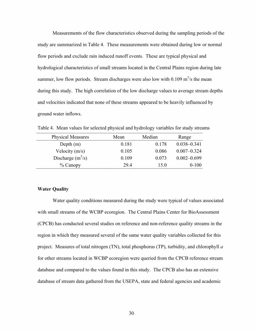
Measurements of the flow characteristics observed during the sampling periods of the

study are summarized in Table 4. These measurements were obtained during low or normal

flow periods and exclude rain induced runoff events. These are typical physical and

hydrological characteristics of small streams located in the Central Plains region during late

summer, low flow periods. Stream discharges were also low with 0.109 m3/s the mean

during this study. The high correlation of the low discharge values to average stream depths

and velocities indicated that none of these streams appeared to be heavily influenced by

ground water inflows.

Table 4. Mean values for selected physical and hydrology variables for study streams

Physical Measures Mean Median Range Depth (m) 0.181 0.178 0.038–0.341

Velocity (m/s) 0.105 0.086 0.007–0.324 Discharge (m3/s) 0.109 0.073 0.002–0.699

% Canopy 29.4 15.0 0-100

Water Quality

Water quality conditions measured during the study were typical of values associated

with small streams of the WCBP ecoregion. The Central Plains Center for BioAssessment

(CPCB) has conducted several studies on reference and non-reference quality streams in the

region in which they measured several of the same water quality variables collected for this

project. Measures of total nitrogen (TN), total phosphorus (TP), turbidity, and chlorophyll a

for other streams located in WCBP ecoregion were queried from the CPCB reference stream

database and compared to the values found in this study. The CPCB also has an extensive

database of stream data gathered from the USEPA, state and federal agencies and academic

31

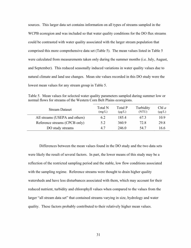
sources. This larger data set contains information on all types of streams sampled in the

WCPB ecoregion and was included so that water quality conditions for the DO flux streams

could be contrasted with water quality associated with the larger stream population that

comprised this more comprehensive data set (Table 5). The mean values listed in Table 5

were calculated from measurements taken only during the summer months (i.e. July, August,

and September). This reduced seasonally induced variations in water quality values due to

natural climate and land use changes. Mean site values recorded in this DO study were the

lowest mean values for any stream group in Table 5.

Table 5. Mean values for selected water quality parameters sampled during summer low or normal flows for streams of the Western Corn Belt Plains ecoregions.

Stream Dataset Total N (mg/L)

Total P (µg/L)

Turbidity (NTU)

Chl a (µg/L)

All streams (USEPA and others) 6.2 185.4 67.3 10.9 Reference streams (CPCB only) 5.2 360.9 72.8 29.8

DO study streams 4.7 246.0 54.7 16.6

Differences between the mean values found in the DO study and the two data sets

were likely the result of several factors. In part, the lower means of this study may be a

reflection of the restricted sampling period and the stable, low flow conditions associated

with the sampling regime. Reference streams were thought to drain higher quality

watersheds and have less disturbances associated with them, which may account for their

reduced nutrient, turbidity and chlorophyll values when compared to the values from the

larger “all stream data set” that contained streams varying in size, hydrology and water

quality. These factors probably contributed to their relatively higher mean values.

32

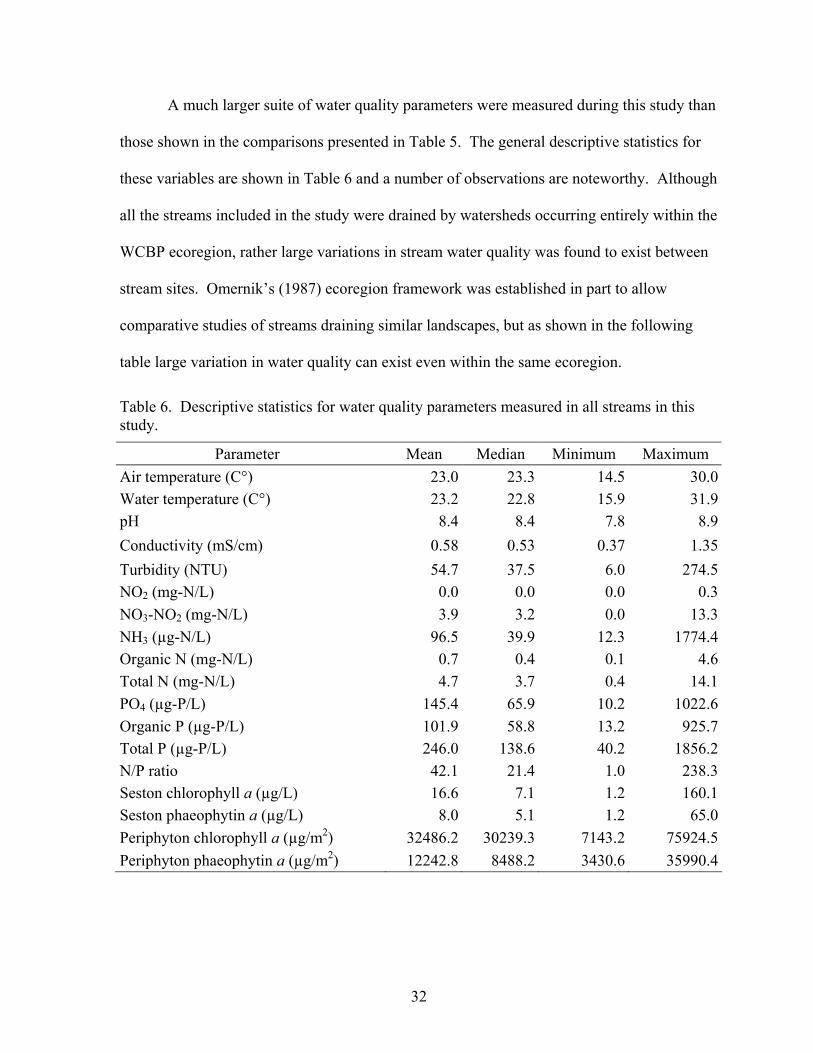
A much larger suite of water quality parameters were measured during this study than

those shown in the comparisons presented in Table 5. The general descriptive statistics for

these variables are shown in Table 6 and a number of observations are noteworthy. Although

all the streams included in the study were drained by watersheds occurring entirely within the

WCBP ecoregion, rather large variations in stream water quality was found to exist between

stream sites. Omernik’s (1987) ecoregion framework was established in part to allow

comparative studies of streams draining similar landscapes, but as shown in the following

table large variation in water quality can exist even within the same ecoregion.

Table 6. Descriptive statistics for water quality parameters measured in all streams in this study.

Parameter Mean Median Minimum Maximum Air temperature (C°) 23.0 23.3 14.5 30.0Water temperature (C°) 23.2 22.8 15.9 31.9pH 8.4 8.4 7.8 8.9Conductivity (mS/cm) 0.58 0.53 0.37 1.35Turbidity (NTU) 54.7 37.5 6.0 274.5NO2 (mg-N/L) 0.0 0.0 0.0 0.3NO3-NO2 (mg-N/L) 3.9 3.2 0.0 13.3NH3 (µg-N/L) 96.5 39.9 12.3 1774.4Organic N (mg-N/L) 0.7 0.4 0.1 4.6Total N (mg-N/L) 4.7 3.7 0.4 14.1PO4 (µg-P/L) 145.4 65.9 10.2 1022.6Organic P (µg-P/L) 101.9 58.8 13.2 925.7Total P (µg-P/L) 246.0 138.6 40.2 1856.2N/P ratio 42.1 21.4 1.0 238.3Seston chlorophyll a (µg/L) 16.6 7.1 1.2 160.1Seston phaeophytin a (µg/L) 8.0 5.1 1.2 65.0Periphyton chlorophyll a (µg/m2) 32486.2 30239.3 7143.2 75924.5Periphyton phaeophytin a (µg/m2) 12242.8 8488.2 3430.6 35990.4

33

Dissolved Oxygen Fluctuation

The DO measurements taken during this study demonstrated three facets of variation:

diel (within a day), daily, and spatial variation (stream to stream). Dissolved oxygen flux

between streams often displayed great variation, fluctuating along a diel cycle with the higher

values occurring in mid afternoon and lows occurring just after midnight of a typical

sampling day (Figure 2). The stream fluxes illustrated in Figure 2 show very different values

and flux amplitudes even though these streams were sampled under very similar climatic and

flow conditions, suggesting that other factors were contributing to the observed DO levels

and flux patterns. The mean DO flux amplitude (range) value for Big Muddy Creek was 8.18

mg/L, which was considerably higher than that the mean amplitude for the West Nishnabotna

River (2.63 mg/L). The DO flux graphs of Figure 2 in many ways typify the variations of

DO flux noted throughout this study and among the different stream systems. However,

some streams displayed anoxic and hypoxic conditions (DO levels zero or > 2.0 mg/L,

respectively) and variations among DO values, flux patterns, productivity and respiration

were apparent when examining the larger set of DO stream sites and values.

34

Big Muddy Creek

0

2

4

6

8

10

12

14

16

18

227 228 229 230 231 232 233 234 235 236 237 238 239 240 241 242

Time (days)

Dis

solv

ed O

xyge

n (m

g/L)

0

5

10

15

20

25

30

35

Temperature (C

)

Dissolved Oxygen Temperature

West Nishnabotna River

0

2

4

6

8

10

12

223 224 225 226 227 228 229 230 231 232 233 234 235 236 237 238 239 240

Time (days)

Dis

solv

ed O

xyge

n (m

g/L)

0

5

10

15

20

25

30

35

Temperature (C

)

Dissolved Oxygen Temperature

Figure 6. Diel DO flux recorded for Muddy Creek (Clay Co., IA from August 16-28, 2001) and the West Nishnabotna River (Shelby Co., IA from August 12-26, 2000).

35

Significant differences among stream variations in DO concentrations were

associated with the DO fluctuations monitored during the deployment periods of individual

streams within the WCBP ecoregion (Table 7). The daily minimums and maximums ranged

from early morning DO minimums of 2.9 to 8.6 mg/L to afternoon DO maximums of

between 6.5 to 17.6 mg/L. At some stream sites, daily fluxes in DO of nearly 10 mg/L were

recorded, although amplitudes of this magnitude were infrequent. The average daily change

in DO between afternoon maximums and nighttime minimums for all the stream sites was

4.3 mg/L. Diel variation at each stream site sometimes displayed daily changes in the flux

pattern of DO and could have very different daily averages even under apparently stable

flows. DO levels exhibited an average daily minimum of 6.0 mg/L during the early morning

hours and increased in concentration to a maximum of 10.3 mg/L in the early to mid

afternoon hours. The average daily DO concentration over the entire study was 7.7 mg/L,

with the range of mean stream site concentrations falling between 4.7 and 11.2 mg/L.

Table 7. Mean, median and range values for DO concentration and saturation values for all streams monitored during this study.

DO (mg/L) DO (% Saturation) Daily DO flux values Mean Median Range Mean Median Range

Maximum 10.3 9.7 6.5 – 17.6 125 118 77 – 228 Minimum 6.0 6.4 2.9 – 8.6 69 71 30 – 97

Mean 7.7 7.9 4.7 – 11.2 89 90 54 – 137 Flux (amplitude) 4.3 3.8 0.9 –10.2 56 49 9 – 138

Because stream temperatures affect DO levels, oxygen saturation values were

examined. Use of saturation values removed the effect of temperature and allowed between-

stream comparisons to be made on a standardized reporting variable. Just as DO

concentration values varied significantly, so did the percent saturation of dissolved oxygen.

36

The average saturation value for the entire study was 89%. The mean stream site DO value

for percent saturation fluctuated from 54% to 137%. During the daytime, daily DO

saturation values rose to an average maximum of 125%. While at night, the average

minimum for the study was 69% saturation. Individual stream sites displayed average

maximum saturation values from 77% up to a very high 228% of saturation. Like the other

mean stream site variables, the mean stream site minimums displayed a similar degree of

variability ranging from 30% to 97%.

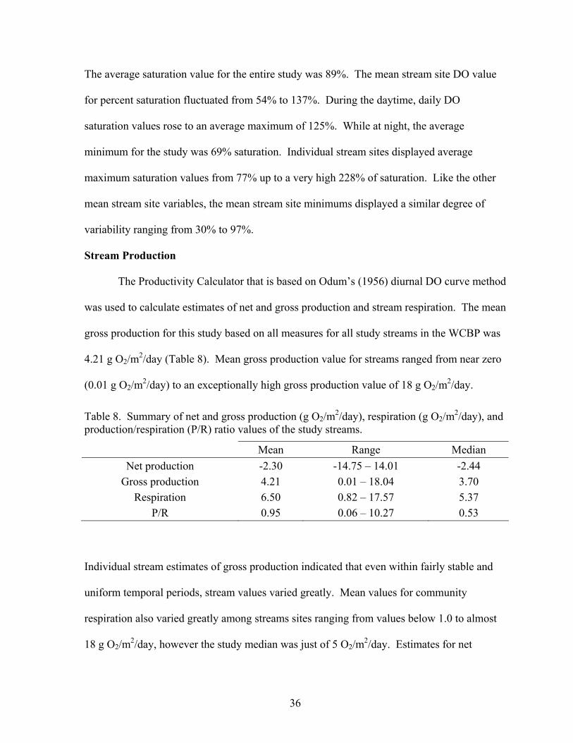
Stream Production

The Productivity Calculator that is based on Odum’s (1956) diurnal DO curve method

was used to calculate estimates of net and gross production and stream respiration. The mean

gross production for this study based on all measures for all study streams in the WCBP was

4.21 g O2/m2/day (Table 8). Mean gross production value for streams ranged from near zero

(0.01 g O2/m2/day) to an exceptionally high gross production value of 18 g O2/m2/day.

Table 8. Summary of net and gross production (g O2/m2/day), respiration (g O2/m2/day), and production/respiration (P/R) ratio values of the study streams.

Mean Range Median Net production -2.30 -14.75 – 14.01 -2.44

Gross production 4.21 0.01 – 18.04 3.70 Respiration 6.50 0.82 – 17.57 5.37

P/R 0.95 0.06 – 10.27 0.53

Individual stream estimates of gross production indicated that even within fairly stable and

uniform temporal periods, stream values varied greatly. Mean values for community

respiration also varied greatly among streams sites ranging from values below 1.0 to almost

18 g O2/m2/day, however the study median was just of 5 O2/m2/day. Estimates for net

37

productivity based on all data using either the mean or median values resulted in negative net

productivity values of more than 2 g O2/m2/day. Consequently, the P/R ratios based on either

mean or median values for respiration and gross production were below 1.00 (0.95 – 0.53)

indicating that in general these streams were autotrophic in nature. While individual site

means for P/R values ranged from 0.06 to 10.27, the vast majority (71%) of streams were

autotrophic and all but two sites had mean P/R values above 2.00.

DO and Production Relationships

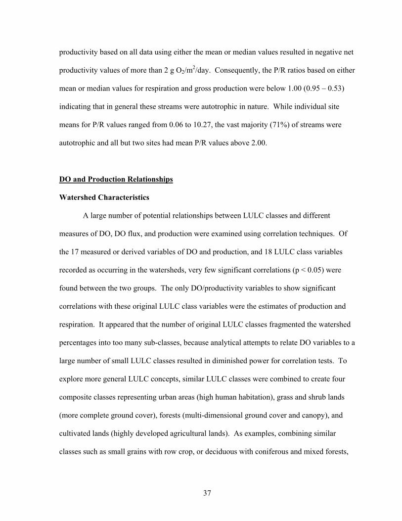
Watershed Characteristics

A large number of potential relationships between LULC classes and different

measures of DO, DO flux, and production were examined using correlation techniques. Of

the 17 measured or derived variables of DO and production, and 18 LULC class variables

recorded as occurring in the watersheds, very few significant correlations (p < 0.05) were

found between the two groups. The only DO/productivity variables to show significant

correlations with these original LULC class variables were the estimates of production and

respiration. It appeared that the number of original LULC classes fragmented the watershed

percentages into too many sub-classes, because analytical attempts to relate DO variables to a

large number of small LULC classes resulted in diminished power for correlation tests. To

explore more general LULC concepts, similar LULC classes were combined to create four

composite classes representing urban areas (high human habitation), grass and shrub lands

(more complete ground cover), forests (multi-dimensional ground cover and canopy), and

cultivated lands (highly developed agricultural lands). As examples, combining similar

classes such as small grains with row crop, or deciduous with coniferous and mixed forests,

38

formed the new LULC classes - total crop and forest, respectively. However, these

composite classes did not show any stronger or different correlation with stream variables

than many of the original variables (Table 9).

Table 9. Significant correlations among large LULC classes and primary production variables. Alpha = 0.05.

Production Estimates - g O2/m2/day LULC Class Number Description Net Respiration Gross

21 + 22 + 23 Urban -0.3483 0.3316 – 41 Deciduous forest – – -0.3298

41 + 42 + 43 Forest – – -0.3335 81 Pasture/Hay 0.3424 – – 82 Row crop -0.3228 0.3112 –

82 + 83 Total crop -0.3259 – –

The r values associated with the significant correlations shown in Table 9 indicted

weak relationships between land use and stream production.. However, most of these

relationships appeared to define plausible causal-based relationships. Certainly, the positive

relationship between the urban LULC class and respiration might be expected in streams

draining urban landscapes. More organic material (e.g. BOD, biological oxygen demand)

may be introduced to these stream systems as a result of urban runoff and sewage treatment

plant effluent, thus increasing community respiration as a result of bacterial decomposition of

the allochthonous organic matter. As increasing respiration rates consume more DO, an

associated decline in net production may be anticipated. Net production did have an inverse

correlation with the percentage of urban LULC in the watersheds. Both forest classes were

found to have inverse correlations with gross production and one hypothesis is that forest

canopy (stream shade) might be a limiting factor of instream gross productivity. Several

39

assumptions would have to be made to accept this hypothesis and even then causality cannot

be determined from these correlations. The first assumption is that the amount of forest in

the watershed is an indicator of the extent of riparian forest along the stream. Secondly, this

riparian forest results in increased canopy cover that causes a decrease in the amount of

sunlight reaching the stream. This decrease in sunlight in turn limits photosynthetic

production. (i.e. gross production).

Relationships between agriculturally developed lands and production exist as well.

Although the positive correlation between pasture/hay and net production seems

counterintuitive, an argument can be made in support of this relationship. Depending on

management practices, manure from grazing animals can lead to increased stream loads of

available phosphorous. Lotic systems in agricultural watershed often receive much of their

phosphorus from manure originating from animal confinement areas and pasturelands. As

nearly all of these streams appear to be phosphorous limited (high N: P ratios), increases in

pasture lands and the potential increase in TP could lead to elevated net production. While

the pasture/hay class showed a positive correlation with net production, the percent row crop

was negatively correlated with net production and positively correlated with respiration. A

possible hypothesis for these relationships is that row crops contributed more organic

material and sediment. While row crop did not show a significant relationship with gross

production, there may have been some limited relationship related to increased suspended

sediment, decreased light penetration and lower gross production which would result in

decreased net production even if the respiration rate remained the same (which it would not

based on the observed relationship in Table 9). It is more likely that the potential increased

transport of organic material to the stream related to increased row cropping resulted in

40

higher respiration rates and subsequently lower net production. All proposed causal

relationship were speculative and the true relationships made be only correlative at best.

Physical Characteristics

Few statistically significant relationships among stream discharge, instream habitat,

substrate composition, temperature and DO/productivity variables were observed using

correlation analyses. Again, the productivity variables tended to better correlate with

measures of physical stream properties than DO and DO flux variables.

No significant relationships were observed among DO/productivity and stream macro

habitat types (i.e. pool, riffle, run), air and water temperatures, and discharge. One might

expect that upstream macrohabitat plays a role in determining DO concentrations associated

with down stream reaches. Our hypothesis was that during low, stable flow periods, large

upstream pools functioning as highly productive run-of-the-river reservoirs or upstream

riffles with their rich periphyton growths contributed large amounts of photosynthically

produced DO that resulted in increases in downstream DO concentrations or flux. However,

no significant correlations between habitat and DO/productivity variables were found.

It would also be expected that surrounding air and water temperatures plays a role in

determining the state of stream oxygen concentrations, and that increases in both air and

water temperature correlates to increases in maximum DO concentration, DO flux, and/or

gross productivity. But again, no such relationships were found between the variables. This

could be a due to sampling procedures that limited air and water temperature measurements

to a two-sample average recorded during the installation of the logger and its removal. Thus,

the observed relationship is between continuous oxygen measurements and essentially

41

“point-in-time” measures of temperature. This temporal discrepancy is the most likely

source for the absence of a significant correlation between temperature and the DO factors.

Discharge was also considered as a factor affecting instream DO, but in this study it

too was revealed no relationship. It was hypothesized that a flushing effect due to increased

discharge would wash out in stream primary producers leading to decreased oxygen content

and lowered production levels. By examining the design of this study, which attempted to

eliminate the impact of runoff events, it should be no surprise that discharge played no

visible role in affecting DO concentrations or productivity.

In examining the significant relationships, substrate was the only physical measure to

correlate with the DO variables. The stream substrate was classified as bedrock, cobble,

gravel, sand, or clay/mud and coded 1 through 5, respectively. The correlations in Table 10

suggest that stream sites with stable substrates (larger mass and weight) also have higher

maximum DO values, higher difference in the maximum and minimum values, and larger

standard deviations in minimum/maximum values. Conversely, sites with bottom substrates

of mostly small substrate sizes (e.g. sand, clay) tended to have lower maximum DO

concentrations and lower DO difference in maximum and minimum daily values. These data

support the premise that large substrates provide stable, higher quality substrate for greater

algae growth and production, which in turn contribute to high DO levels and larger flux.

Table 10. Significant correlations between DO variables and stream substrate. Substrate size classes varied from 1 (bedrock), to 2 (cobble) on down to 5 representing clay/mud. Alpha = 0.05.

DO variables (daily means for deployment periods) Maximum Difference Std Dev % Max % Difference % Std Dev

Substrate class -0.3282 -0.3512 -0.3828 -0.3835 -0.3519 -0.3745

42

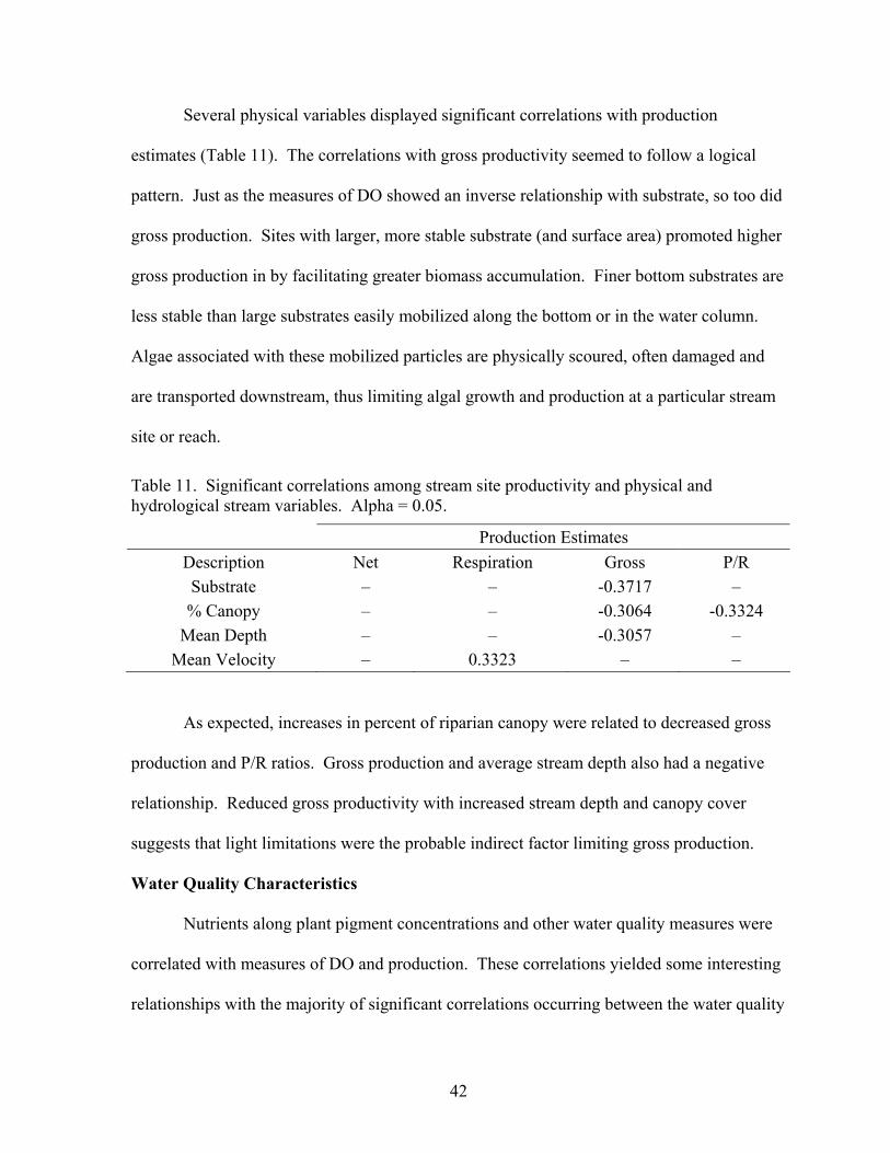
Several physical variables displayed significant correlations with production

estimates (Table 11). The correlations with gross productivity seemed to follow a logical

pattern. Just as the measures of DO showed an inverse relationship with substrate, so too did

gross production. Sites with larger, more stable substrate (and surface area) promoted higher

gross production in by facilitating greater biomass accumulation. Finer bottom substrates are

less stable than large substrates easily mobilized along the bottom or in the water column.

Algae associated with these mobilized particles are physically scoured, often damaged and

are transported downstream, thus limiting algal growth and production at a particular stream

site or reach.

Table 11. Significant correlations among stream site productivity and physical and hydrological stream variables. Alpha = 0.05.

Production Estimates Description Net Respiration Gross P/R Substrate – – -0.3717 – % Canopy – – -0.3064 -0.3324

Mean Depth – – -0.3057 – Mean Velocity – 0.3323 – –

As expected, increases in percent of riparian canopy were related to decreased gross

production and P/R ratios. Gross production and average stream depth also had a negative

relationship. Reduced gross productivity with increased stream depth and canopy cover

suggests that light limitations were the probable indirect factor limiting gross production.

Water Quality Characteristics

Nutrients along plant pigment concentrations and other water quality measures were

correlated with measures of DO and production. These correlations yielded some interesting

relationships with the majority of significant correlations occurring between the water quality

43

measures and the DO values. A number of basic statistics (e.g. mean, median) for the raw

DO values and percent saturation DO values were compared to the water quality variables.

Because no mode values were calculated for the percent saturation values, the mode values

calculated for the raw DO values were not included the correlation analysis. The raw DO

statistics and the percent DO saturation statistics yielded very similar correlations with the

same water quality parameters. Thirty-two significant correlations were observed for the raw

DO variables along with 34 correlations for the percent saturation variables. Out of these

significant correlations, 29 were between the same water quality variable and the matching

statistical measure for the raw DO and percent saturation variables, suggesting that either the

variables based on raw DO values or saturation values could be used to examine relationships

between DO and other water quality variables as illustrated in Table 12. This table shows

that the correlation values and sign relationships between raw and saturation derived

variables and nitrate/nitrite, N:P ratios and chlorophyll a concentrations are nearly identical.

In addition, the examination of correlation matrix for raw and percent saturation variables

showed that there were virtually no differences between these variables as they were highly

correlated. The mean difference between correlation pairs (raw verses % saturation) for the

29 common DO variables was only 0.005. Therefore, in order to eliminate some of the

redundancy in the analyses, only the correlations between the water quality variables and the

raw DO statistics were examined in any detail.

44

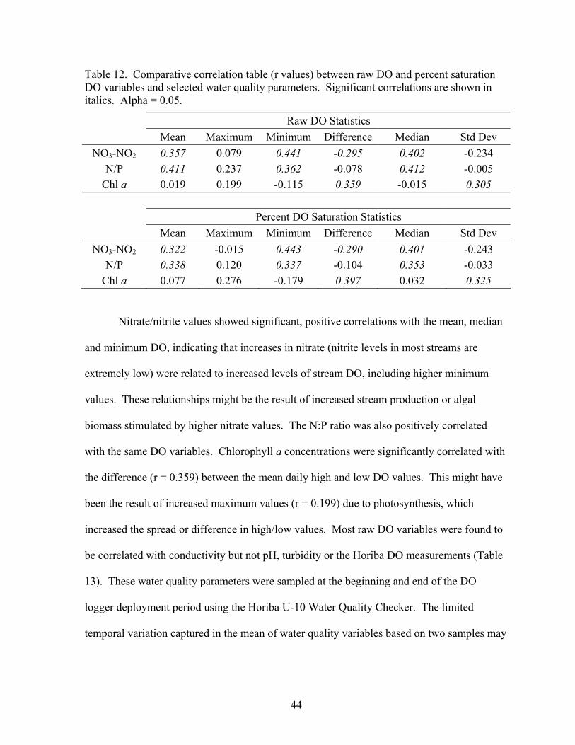
Table 12. Comparative correlation table (r values) between raw DO and percent saturation DO variables and selected water quality parameters. Significant correlations are shown in italics. Alpha = 0.05.

Raw DO Statistics Mean Maximum Minimum Difference Median Std Dev

NO3-NO2 0.357 0.079 0.441 -0.295 0.402 -0.234 N/P 0.411 0.237 0.362 -0.078 0.412 -0.005

Chl a 0.019 0.199 -0.115 0.359 -0.015 0.305

Percent DO Saturation Statistics Mean Maximum Minimum Difference Median Std Dev

NO3-NO2 0.322 -0.015 0.443 -0.290 0.401 -0.243 N/P 0.338 0.120 0.337 -0.104 0.353 -0.033

Chl a 0.077 0.276 -0.179 0.397 0.032 0.325

Nitrate/nitrite values showed significant, positive correlations with the mean, median

and minimum DO, indicating that increases in nitrate (nitrite levels in most streams are

extremely low) were related to increased levels of stream DO, including higher minimum

values. These relationships might be the result of increased stream production or algal

biomass stimulated by higher nitrate values. The N:P ratio was also positively correlated

with the same DO variables. Chlorophyll a concentrations were significantly correlated with

the difference (r = 0.359) between the mean daily high and low DO values. This might have

been the result of increased maximum values (r = 0.199) due to photosynthesis, which

increased the spread or difference in high/low values. Most raw DO variables were found to

be correlated with conductivity but not pH, turbidity or the Horiba DO measurements (Table

13). These water quality parameters were sampled at the beginning and end of the DO

logger deployment period using the Horiba U-10 Water Quality Checker. The limited

temporal variation captured in the mean of water quality variables based on two samples may

45

have prevented the identification of significant correlations with the DO variables that were

measured at both a daily (diel) and longer time sequence. The single daily measures of DO

were predominantly taken during the afternoon hours when oxygen production is at its

highest. This most likely resulted in the significant positive correlation with maximum DO

and none of the other DO variables. During periods of increased oxygen production, streams

will become less acidic as primary producers remove carbon from the water for

photosynthesis. This is shown by the significant positive correlation between pH and the DO

flux variables. The fact that pH correlated better with the measures of DO flux was because

pH follows a cyclic pattern that was expressed by these variables. Conductivity exhibited

significant negative correlations with the DO variables. Conductivity is closely correlated

with total dissolved solids, which are typically comprised of organic substances, a potential

source of BOD. The BOD may have then reduced DO concentrations. However, the

positive relationship between DO and stream conductivity is purely conjecture and based

upon several sound but unsubstantiated assumptions.

Table 13. Correlation table (r values) between DO and water quality variables. Significant correlations are shown in italics. Alpha = 0.05.

Raw DO Statistics Mean Maximum Minimum Differences Median Std Dev

pH -0.016 0.206 -0.191 0.362 -0.114 0.325 Conductivity -0.352 -0.300 -0.367 -0.027 -0.361 -0.087

Turbidity -0.103 -0.066 0.020 -0.044 -0.059 -0.103 DO (single daily measure) 0.281 0.332 0.191 0.222 0.251 0.269

Examination of significant correlations between DO and the measures of nitrogen

suggested that nitrogen does not affect DO flux. Most nitrogen species except for ammonia

were positively correlated with minimum, mean and median DO (Table 14). Increases in

46

nitrate as well as inorganic N and TN would raise the level of minimum DO but not

maximum, thus increasing the mean and median DO (see Tables 13 and14). Also, the rise in

only the minimum DO was the apparent cause for the maximum/minimum difference to

display a negative relationship with nitrate. The correlations with the inorganic component

of nitrogen followed the same pattern as those with nitrate largely because the dominant

constituent of inorganic nitrogen is nitrate. Total nitrogen also showed a positive relationship

with the minimum and median values of DO. The median relationship was no doubt a

byproduct of the increase in the minimum DO measure. Ammonia was negatively correlated

with minimum, mean and median DO levels; the strong correlation (r=-0.467) was between

mean DO and ammonia. These negative relations might be the result of several instream

processes. As Peterson et al. (2001) showed, ammonia is removed from the stream and

assimilated by photosynthetic plants and heterotrophic organisms. In addition, microbial

organisms living in anoxic conditions within the streambed or in deep pool reaches may

produce ammonia through the reduction of nitrogen.

Table 14. Correlation table (r values) between DO and nitrogen variables. Significant correlations are shown in italics. Alpha = 0.05.

Raw DO Statistics Mean Maximum Minimum Differences Median Std Dev

NO3-NO2 0.357 0.079 0.441 -0.295 0.402 -0.234 NO2 0.072 0.033 0.109 -0.120 0.097 -0.106 NH3 -0.467 -0.253 -0.430 0.035 -0.455 -0.010

Inorganic N 0.338 0.073 0.417 -0.292 0.381 -0.235 Organic N 0.118 0.141 0.038 0.161 0.105 0.157

Total N 0.267 0.023 0.359 -0.270 0.316 -0.242

47

Few correlations were found between phosphorus variables and the various measures

of DO (Table 15). All significant correlations with phosphorus were negative. Increases in

P04 concentrations resulted in lower maximum, mean and median DO levels. The

relationships with the median and average DO values were most likely a consequence of the

negative relationship with maximum DO. Total phosphorus also exhibited a negative

relationships with mean DO levels. These data suggest that increases in stream phosphorus

values could lead to lower stream DO levels. This idea is supported by the observed

correlations between nitrogen and phosphorus ratios (N/P) and mean, minimum and median

DO.

Table 15. Correlation table (r values) between DO and phosphorus variables and the N:P ratio. Significant correlations are shown in italics. Alpha = 0.05.

Raw DO Statistics Mean Maximum Minimum Difference Median Std Dev

N:P 0.411 0.237 0.362 -0.078 0.412 -0.005 PO4 -0.390 -0.400 -0.203 -0.220 -0.346 -0.259

Organic P -0.059 -0.022 -0.000 0.052 -0.027 -0.033 Total P -0.294 -0.273 -0.132 -0.130 -0.244 -0.184

All significant correlations between N:P and the DO statistics were positive

indicating that as the N:P ratio increased so did the average, median, and minimum DO

statistics (Table 15). However, the most important relationship with the N:P ratio is the

positive relationship with minimum DO values. High N:P values indicates that the system is

likely to be phosphorus limited, meaning that in these systems as N:P increase, DO values

increase and phosphorus decreases. What becomes apparent after examining these

correlations between DO and phosphorus is that limiting, phosphorus is not controlling the

increase or fluctuation of DO, but appears to be related to decreases in DO.

48

Few significant correlations between water quality variables and estimates of stream

production and respiration were observed in this study. Those few water quality variables

that did show a significant correlation with at least one stream productivity variable are

included in Table 16. The average of the two instantaneous measures of DO (single point in

time measures) taken with the Horiba U-10 Water Quality Checker at the beginning and end

of the logger deployment period correlated fairly well with gross production. This

relationship might have been the result of the fact that high productivity rates (gross

production) often occur in mid- to late afternoon with increased solar radiation and water

temperatures, which coincided with the typical mid-day measurement of stream DO with the

Horiba. Since gross production is a major component in the calculation of both net

production and the P/R ratio, it is reasonable to assume that correlations between these

estimates and instantaneous DO were a result of the relationship between gross productivity

and the DO variable. The positive relationship between pH and gross production was

assumed to be related to the uptake of carbon mostly from CO2 as a result of photosynthesis

and thus a reduction in carbonic acid.

Table 16. Correlations (r values) between the water quality variables and estimates of stream production, respiration and the P/R ration. Significant correlations are shown in italics. Alpha = 0.05.

Production and Respiration Variables Respiration Gross production Net production P/R ratio

pH 0.131 0.333 0.118 0.209 Conductivity 0.372 0.084 -0.269 -0.191

Turbidity -0.209 -0.109 0.129 0.116 DO (single point in time) -0.182 0.447 0.313 0.391

NH3 0.391 -0.186 -0.503 -0.402

49

Ammonia was the only nutrient variable to significantly correlate with the estimates

of production and respiration. It appears that increases in stream ammonia are related to

increases stream respiration, but it is unclear what this relationship represents. A similar

relationship was observed between ammonia and minimum stream DO (Table 14) where

increases in ammonia were correlated to decreases in DO. These two relationships suggest

that increased ammonia values are related to increased respiration that leads to lower

instream DO level (al least lower minimums). One explanation might be that increases in

heterotrophic activity results in increased respiration rates, and ammonia levels rise as a

result of the uptake and conversion of nitrate to ammonia by the same heterotrophic

community.

Seston and Benthic Chlorophyll

No benthic chlorophyll or phaeophytin variables were significantly correlated with

any of the DO variables, suggesting that periphyton biomass was not related to DO levels in

these streams. This does not mean that benthic chlorophyll does not contribute to instream

oxygen levels, but rather that no relationships were observed during these low-flow sampling

events. Additionally, there were few significant correlations found between sestonic

chlorophyll concentrations and stream DO (Table 17). Sestonic chlorophyll, phaeophytin

and the chlorophyll/phaeophytin ratio were positively correlated with one or both of the

measures of DO flux amplitude (e.g.the difference and standard deviation variables).

Overall, these rather weak relationships suggest that as sestonic algal biomass increases so

does DO flux, probably because of increased photosynthetic processes. Phaeophytin, a

breakdown product of chlorophyll, reflect episodes of high algal growth. When the

proportion of chlorophyll to phaeophytin is high, algal populations experience high growth

50

rates or low senescence. The positive correlation between the difference variable and the

chlorophyll/phaeophytin ratio indicates that growth in suspended algae populations lead to an

increase in DO fluctuations.

Table 17. Correlation table (r values) between DO and benthic algal pigment variables. Significant correlations are shown in italics. Alpha = 0.05.

Raw DO Statistics Mean Maximum Minimum Difference Median Std Dev

Chlorophyll a 0.019 0.199 -0.115 0.359 -0.015 0.305 Phaeophytin a 0.029 0.169 -0.106 0.285 -0.009 0.245

Chlorophyll/Phaeophytin Ratio 0.012 0.209 -0.084 0.386 -0.012 0.341

.1

1

10

100

1000

.1 1 10 100 1000Fine Sediment Chlorophyll (ug/cm2)

Larg

e S

ubst

rate

Chl

orop

hyll

(ug/

cm2)

Figure 2. Scatter plot of chlorophyll a concentration obtained from samples taken from large (e.g. cobble, logs) and fine (e.g. sand, silt) substrates within the same stream sites (n = 44)

51

Co-collected benthic algal collections were analyzed to determine if periphyton

communities colonizing different substrates were similar or different. If substrate size did

promote the establishment of different periphyton communities then comparisons of sites

with different bottom substrates would have to be evaluated with care. Data collected by

Iowa Department of Natural Resources (IDNR) and provided for this effort were analyzed to

evaluate periphyton relationships between communities occurring on large and fine

substrates found at the same sites. A scatter plot (Figure 17) of these data suggests a weak

positive relationship between benthic chlorophyll a concentrations on large verses small

substrates. However, both regression and correlation analyses indicated that there was no

statistically significant relationship between these periphyton concentrations.

Macroinvertebrates

Again using IDNR productivity, DO and macroinvertebrate data, a number of

analyses were preformed. Examination of the Spearman correlation matrix for these data

revealed only two significant correlations when examining macroinvertebrate variables and

DO and productivity measures. No significant correlations (Spearman-rank correlation,

alpha = 0.05) were observed between percent EPT (Ephemeroptera, Plecoptera, Trichoptera)

and DO or productivity variables. However, both mean daily respiration and consequently

net production were correlated with IDNR’s modification of the Hilsenhoff Biotic Index

(Hilsenhoff 1987). A significant positive correlation (r = 0.546) was found between the

modified Hilsenhoff Biotic Index scores (possible range of 1 to 10) and respiration indicating

that increases in stream respiration rates negatively affected the macroinvertebrate

community. A scatter plot with both a regression line and smoothed fit line was constructed

and the results are shown in Figure3. A threshold affect was apparent between a respiration

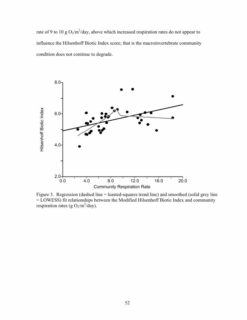
52

rate of 9 to 10 g O2/m2/day, above which increased respiration rates do not appear to

influence the Hilsenhoff Biotic Index score; that is the macroinvertebrate community

condition does not continue to degrade.

2.0

4.0

6.0

8.0

0.0 4.0 8.0 12.0 16.0 20.0Community Respiration Rate

Hils

enho

ff B

iotic

Inde

x

Figure 3. Regression (dashed line = leasted-squares trend line) and smoothed (solid grey line = LOWESS) fit relationships between the Modified Hilsenhoff Biotic Index and community respiration rates (g O2/m2/day).

53

LITERATURE CITED

APHA, AWWA, and WEF. 1998. Standard methods for the examination of water and wastewater, 20th ed. APHA, Washington, D.C. Bara, T.J., comp. ed. 1994. Multi-resolution land characteristics consortium--documentation notebook. [Environmental Monitoring and Assessment Program-Landscape Characterization, Contract 68-DO-0106]: Research Triangle Park, N.C., ManTech Environmental Technology, Inc. [variously paginated]. BioDevices Corp. 1999. AQUA 2002 Dissolved oxygen and temperature data logger instruction manual, ver. 1.4. Ames, IA: 15. Bott, T.L., J.T. Brock, C.E. Cushing, S.V. Gregory, D. King, and R.C. Peterson. 1978. A comparison of methods for measuring primary productivity and community respiration in streams. Hydrobiologia 60:3-12. Bott, T.L. 1996. Primary Productivity and Community Respiration. Methods in Stream Ecology. F.R. Hauer and G.A. Lamberti, Academic Press: 533-556. Bouchard, R.W. and J.A. Anderson, 2001. Description and Protocol for Two Quantitative Periphyton Samplers Used for Multihabitat Stream Sampling Documentation of Periphyton Sampling Techniques Employed by the Central Plains Center for BioAssessment. http://www.cpcb.ku.edu/datalibrary/html/library/index.htm#techdocs Chapman, S.S., J.M. Omernik, J.A. Freeouf, D.G. Huggins, J.R. McCauley, C.C. Freeman, G. Steinauer, R.T. Angelo, and R.L. Schlepp. 2001. Ecoregions of Nebraska and Kansas (color poster with map, descriptive text, summary tables, and photographs): Reston, Virginia, U.S. Geological Survey (map scale 1:1,950,000). Dodds, W.K., J.R. Jones, and E.B. Welch. 1998. Suggested classification of stream trophic state: distributions of temperate stream types by chlorophyll, total nitrogen, and phosphorus. Water Resources 32(5):1455-1462. Dodds, W.K. and E.B. Welch. 2000. Establishing nutrient criteria in streams. Journal of the North American Benthological Society 19(1):186-196. Ebina, J., T. Tsuyoshi, and T. Shirai. 1983. Simultaneous determination of total nitrogen and total phosphorus in water using peroxodisulfate oxidation. Water Research 17:1721–1726. Elmore, H.L. and W.F. West. 1961. Effects of water temperature on stream reaeration. Journal of the Sanitary Engineering Division ASCE. 91:59-71. Fleituch, T. 1999. Responses of benthic community metabolism to abiotic factors in a mountain river in southern Poland. Hydrobiologia 380: 27-41.

54

Horne, A.J. and C.R. Goldman. 1994. Limnology. New York, McGraw-Hill. Kelly, M.G., G.M. Hornberger, and B.J. Cosby. 1974. Continuous automated measurement of rates of photosynthesis and respiration in an undisturbed river community. Limnology and Oceanography 19(2):305-312. Konsinski, R.J. 1984. A comparison of the accuracy and precision of several open-water oxygen productivity techniques. Hydrobiologia 119(2):139-148. Kotak, B.G., E.E. Prepas, and S.E. Hrudey. 1994. Blue green algal toxins in drinking water supplies: Research in Alberta. Lake Line 14:37-40. Lamberti, G.A. 1996. The niche of benthic food webs in freshwater ecosystems. Algal Ecology, Freshwater Benthic Ecosystems. Stevenson, R.J., M.L. Bothwell, and R.L. Lowe, Academic Press: 553-564. Maidment, D.R., Ed. 1993. Handbook of Hydrology. New York, McGraw-Hill. Marzolf, E.R., P.J. Mulholland, and A.D. Steinman. 1994. Improvements to the diurnal upstream-downstream dissolved oxygen change technique for determining whole-stream metabolism in small streams. Canadian Journal of Fisheries and Aquatic Sciences 51:1591-1599. Matson, P.A., W.J. Parton, A.G. Power, and M.J. Swift. 1997. Agricultural intensification and ecosystem properties. Science 277:504-509. Minshall, G.W. 1978. Autotrophy in stream ecosystems. BioScience 28:767-771. Naiman, R.J. and R.E. Bilby, Eds. 1998. River Ecology and Management: Lessons from the Pacific Costal Ecoregion. New York, Springer. National Climatic Data Center. lwf.ncdc.noaa.gov/oa/ncdc.html O'Connor, D.J. and W.E Dobbins. 1956. Mechanism of reaeration in natural streams. Journal of the Sanitary Engineering Division, ASCE 123:641-684. Odum, H.T. 1956. Primary production in flowing waters. Limnology and Oceanography 1(2):102-117. Omernik, J.M. 1987. Ecoregions of the conterminous United States. Annals of the Association of American Geographers 77(1):118-125. Owens, M., R.W. Edwards, and J.M. Gibbs. 1964. Some reaeration studies in streams. International Journal of Air and Water Pollution 8:469-486.

55

Peterson, B.J., W.M. Wollheim, P.J. Mulholland, J.R. Webster, J.L. Meyer, J.L. Tank, E. Martí, W.B. Bowden, H.M. Valett, A.E. Hershey, W.H. McDowell, W.K. Dodds, S.K. Hamilton, S. Gregory, and D.D. Morrall. 2001. Control of nitrogen export from watersheds by headwater streams. Science 292:86-90. Palmstrom, N.S., R.E. Carlson, and G.D. Cooke. 1988. Potential links between eutrophication and formation of carcinogens in drinking water. Lake and Reservoir Manage. 4:1-15. Sharpley, A., B. Foy, and P. Withers. 2000. Practical and innovative measures for the control of agricultural phosphorus losses to water: an overview. Journal of Environmental Quality 29(1):1-9. Smith, V.H., G.D. Tilman, and J.C. Nekola. 1999. Eutrophication: impacts of excess nutrients on freshwater, marine, and terrestrial ecosystems. Environmental Pollution. Swoffer Instruments, Inc. Instructions for Operation and Maintenance of 2100 Indicator. Seattle, WA. Uehlinger, U. and M.W. Naegeli. 1998. Ecosystem metabolism, disturbance, and stability in a prealpine gravel bed river. Journal of the North American Benthological Society 17(2):165-178. USEPA. 1996. National Water Quality Inventory 1996 Report to Congress. EPA-841-R-97-008. U.S. Washington, D.C, Environmental Protection Agency, Office of Water. USEPA. 1998. National Strategy for the Development of Regional Nutrient Criteria. EPA-822-R-98-002. Washington, D.C., U. S. Environmental Protection Agency, Office of Water: 45. USEPA. 2000. Nutrient Criteria Technical Guidance Manual: Rivers and Streams. EPA-822-B-00-002. Washington, D.C., U. S. Environmental Protection Agency, Office of Water: 152. Vannote, R.L., G.W. Minshall, K.W. Cummins, J.R. Sedell, and C.E. Cushing. 1980. The River Continuum Concept. Canadian Journal of Fisheries and Aquatic Sciences 37: 130-137. Welch, E.B. 1992. Ecological Effects of Wastewater. Chapman and Hall, London. Wilcock, R.J. 1982. Simple predictive equations for calculating stream reaeration rate coefficients. New Zealand Journal of Sciences 25:53-56. Wilcock, R.J., G.B. McBride, J.W. Nagels, and G.L. Northcott. 1995. Water quality in a polluted lowland stream with chronically depressed dissolved oxygen: causes and effects. New Zealand Journal of Marine and Freshwater Research 29:277-288.

56

Wiley, M.J., L.L. Osborne, and R.W. Larimore. 1990. Longitudinal structure of an agricultural prairie river system and its relationship to current stream ecosystem theory. Canadian Journal of Fisheries and Aquatic Sciences 47:373-383. Young, R.G. and A.D. Huryn. 1999. Effects of land use on stream metabolism and organic matter turnover. Ecological Applications 9(4):1359-1376.