dissipative particle dynamics modeling of red blood...

Dissipative particledynamics modelingof red blood cells

6

D. A. Fedosov#, B. Caswell†, G. E. Karniadakis#

Division of Applied Mathematics#

Division of Engineering†

Brown UniversityProvidence

Capsules and red blood cells suspended in various flows exhibit a rich dy-namics due to the deformability of the enclosing membranes. To accuratelycapture statics and dynamics, mechanical models of the membrane must beavailable incorporating shear elasticity, bending rigidity, and membrane vis-cosity. In the approach described in this chapter, the membrane of a red bloodcell is modeled as a network of interconnected nonlinear springs emulating themembrane spectrin network. Dissipative forces in the network mimic the ef-fect of the lipid bilayer. The macroscopic elastic properties of the networkare analytically related to the spring parameters to circumvent ad-hoc ad-justment. Chosen parameters values yield model membranes that reproduceoptical tweezer stretching experiments. When probed with an attached os-cillating microbead, predicted viscoelastic properties are in good agreementwith experiments using magnetic optical twisting cytometry. In shear flow, redblood cells respond by tumbling at low shear rates and tank-treading at highshear rates. In transitioning between these regimes, the membrane exhibitssubstantial deformation controlled largely by flexural stiffness. Raising themembrane or internal fluid viscosity shift the transition threshold to highershear rates and reduces the tank-treading frequency. Simulations reveal thata purely elastic membrane model devoid of a viscous properties cannot ade-quately capture the cell dynamics. Results are presented to demonstrate thedependence of transition thresholds from biconcave to parachute shapes incapillary flow on the cell properties and the mean flow velocity.

1

2 Computational Hydrodynamics of Capsules and Cells

6.1 Introduction

Red blood cells are soft biconcave capsules with an average diameter 7.8 µmand an interior viscous liquid enclosed by a viscoelastic membrane. The cellmembrane consists of a nearly incompressible lipid bilayer attached to a spec-trin protein network held together by short actin filaments known as thecytoskeleton. This membrane structure ensures the integrity of the cell innarrow capillaries whose cross-section is smaller than the size of the biconcavedisk (e.g., Fung 1993). Consistent with the spectrin cytoskeleton structure,the membrane can be modeled as a network of viscoelastic springs mediatingelastic and viscous response. Flexural stiffness can be introduced as a networkbending energy, and constraints on the surface area and volume can be im-posed to enforce the area incompressibility of the lipid bilayer and the volumeincompressibility of the interior fluid.

A number of theoretical and numerical analyses have sought to describecell behavior and deformation in a variety of flows. Examples include mod-els of ellipsoidal cells enclosed by viscoelastic membranes (e.g., Abkarian etal. 2007, Skotheim & Secomb 2007), numerical models based on shell theory,(e.g., Fung 1993, Eggleton & Popel 1998, Pozrikidis 2005), and discrete de-scriptions at the spectrin protein level (e.g., Discher et al. 1998, Li et al. 2005)or at a mesoscopic level (e.g., Noguchi & Gompper 2005, Dupin et al. 2007,Pivkin & Karniadakis 2008). The membranes of healthy red blood cells ex-hibit nonlinear elastic response in steady stretching and viscous response indynamic testing. Most existing membrane models incorporate only the elasticresponse. Fluid-and solid-like models demand high computational costs dueto the strong coupling of solid mechanics and fluid flow.

Semicontinuum models of deformable cells employ boundary-element,immersed-boundary, and front-tracking methods to combine a discrete mem-brane representation with the interior and exterior flow (e.g., Eggleton &Popel 1998, Pozrikidis 2005). A membrane is described by a set of point par-ticles whose motion is coupled to a flow computed on an Eulerian grid. Mostmodels assume that the fluid viscosities are equal and ignore thermal fluctua-tions (e.g., Noguchi & Gompper 2005). Modeling a cell at the spectrin-proteinlevel is constrained by high computational cost.

Mesoscopic modeling of viscoelastic capsules and red blood cells are cur-rently being developed to describe three-dimensional motion (e.g., Noguchi &Gompper 2005, Dupin et al. 2007, Pivkin & Karniadakis 2008). Noguchi &Gompper (2005) simulated the deformation of vesicles enclosed by viscoelasticmembranes using the method of multi-particle collision dynamics (e.g., Mal-evanets & Kapral 1999). Dupin et al. (2007) combined a lattice-Boltzmannmethod (e.g., Succi 2001) with a discrete membrane representation neglect-

Chapter 6 Dissipative particle dynamics modeling of red blood cells 3

ing the membrane viscosity and the occurrence of thermal fluctuations. Theimplementation smears the sharp interface between the external and internalfluid requited by the impenetrability of the membrane.

The elasticity of the red blood cell membrane is attributed to a spectrinnetwork of approximately 27×103 nodes. The population number was reduced(coarse-grained) by Pivkin & Karniadakis (2008) by employing a dissipativeparticle dynamics (DPD) approach to represent cell membranes with networksof only 500 DPD particles connected with springs. (e.g., Hoogerbrugge &Koelman 1992) Their model is the starting point for the work discussed inthis chapter.

First, a theoretical analysis will be presented for a membrane networkmodel exhibiting specified macroscopic membrane properties without param-eter adjustment. The predicted cell mechanical properties will be comparedwith optical tweezers stretching experiments by Suresh et al. (2005), andthe predicted rheological properties will be compared with magnetic opticaltwisting cytometry experiments by Puig-de-Morales-Marinkovic et al. (2007).Red blood dynamics in shear flow showing tumbling and tank-treading willbe studied in detail with a view to delineating the effect of the membraneshear moduli, bending rigidity, external, internal, and membrane viscosities.Simulations of cell motion in Poiseuille flow will confirm that the biconcave-to-parachute transition depend on the flow strength and membrane properties.Comparison with available experiments will demonstrate that the computa-tional model is able to accurately describe realistic red blood cell motion.

Comparison of the numerical simulations with theoretical predictionsby Abkarian et al. (2007), Skotheim & Secomb (2007), and others will revealdiscrepancies suggesting that the current theoretical models are only qualita-tively accurate due to strong simplifications.

6.2 Mathematical framework

In the theoretical model, the membrane of a red blood cell is represented bya viscoelastic network. The motion of the internal and external fluids is de-scribed by the method of dissipative particle dynamics (DPD) (e.g., Hooger-brugge & Koelman 1992). The membrane model is sufficiently general tobe used with other simulation techniques, such as Brownian dynamics, lat-tice Boltzmann, multiparticle collision dynamics, and the immerse-boundarymethod.


6.2.1 Dissipative particle dynamics

Dissipative particle dynamics (DPD) is a mesoscopic simulation technique forcomputing the flow of complex fluids. A DPD system of N particles representslumps of atoms or molecules described by the particle position, ri, velocity,vi, and mass mi, where i = 1, . . . , N . Particle interactions are mediated byconservative (C), dissipative (D), and random (R) interparticle forces givenby

FCij = FC

ij (rij) rij , FDij = −γ ωD(rij) (vij · rij)rij ,

FRij = σ ωR(rij)

ξij√dt

rij , (6.2.1)

where rij is the distance between the ith and jth particle, rij = rij/rij isa unit vector, rij = |rij |, and vij = vi − vj . The coefficients γ and σ arethe amplitudes of the dissipative and random forces, and the factors ωD andωR are weights. The random force definition employs normally distributedrandom variables ξij with zero mean, unit variance, and pairwise symmetry,ξij = ξji. The forces vanish beyond a cutoff radius, rc, which defines the DPDlength scale.

A typical conservative force is

FCij (rij) =

{

aij(1 − rij/rc) for rij ≤ rc,0 for rij > rc,

(6.2.2)

where ai and aj are conservative force coefficients for the ith and jth particle.The random force weight function ωR(rij) is chosen to be

ωR(rij) =

{

(1 − rij/rc)m for rij ≤ rc,

0 for rij > rc.(6.2.3)

In the original DPD method, m was set to unity. Different exponent values canbe used to alter the fluid viscosity and increase the Schmidt number Sc = ν/D,where D is the self-diffusion,and ν = µ/ρ is the kinematic viscosity (e.g., Fanet al. 2006, 2008).

Temperature control is achieved by balancing random and dissipativeforces according to the fluctuation-dissipation theorem,

ωD(rij) =[

ωR(rij)]2

, σ2 = 2γkBT, (6.2.4)

where T is the equilibrium temperature and kB is the Boltzmann constant(e.g., Espanol & Warren 1995).


The particles move in space according to the Newton’s second law ofmotion,

dri

dt= vi,

dvi

dt=

1

mi

∑

j 6=i

Fij , (6.2.5)

where ri is the particle position and Fij is the force exerted on the ith by thejth particle. The particle equation of motion is integrated with the velocityVerlet algorithm (e.g., Allen & Tildesley 1987).

6.2.2 Mesoscopic viscoelastic membrane model

The cell membrane is represented by a two-dimensional curved triangulatednetwork defined by Nv vertices, xi, connected by Ns springs (edges) to formNt triangular faces, where i = 1, . . . , Nv. The total energy of the networkconsists of an in-plane elastic energy, a viscous dissipation energy (IP), abending energy (B), a surface area energy (A), and a volume energy (V),

V ({xi}) = VIP + VB + VA + VV . (6.2.6)

The individual energy components are discussed in this section.

Elastic energy and viscous dissipation

The in-plane elastic energy is given by

VIP =∑

j=1,...,Ns

[UIPS(ℓj) + UIPV (∆vj)] +

Nt∑

k=1

Cq

Aqk

, (6.2.7)

where IPS stands for the in-plane spring energy and IPV stands for the in-plane viscous dissipation. The first sum in (6.2.7) expresses the contributionof viscoelastic springs; ℓj is the length of the jth spring and ∆vj is the relativevelocity of the spring end points. The second sum expresses a stored elasticenergy assigned to each triangular patch; Ak is the area of the kth triangle.The constant Cq and exponent q will be defined.

We employ the worm-like chain (WLC) model alone or in combinationwith a stored elastic energy (WLC-C) or a power function (POW) potential(WLC-POW). The WLC energy is given by

UWLC =kBTℓm

4p

3x2 − 2x3

1 − x. (6.2.8)

where x = ℓ/ℓm ∈ (0, 1), ℓm is the maximum spring extension, and p is thepersistence length. The power-function energy is given by

UPOW =kp

(n − 1)ℓn−1, (6.2.9)


where kp is a spring constant and n is a specified exponent.

Attractive forces exerted by WLC springs cause element compression.The second term in the WLC-C model (6.2.7) contributes an elastic energythat tends to expand the area. The equilibrium state of a single triangularplaquette with WLC-C energy defines an equilibrium spring length, ℓ0. Arelationship between the WLC spring parameters and Cq can be obtained bysetting the Cauchy stress derived from the virial theorem to zero (e.g., Allen& Tildesley 1987),

CWLCq =

√3Aq+1

0

4pqℓmkBT

4x20 − 9x0 + 6

1 − x0, (6.2.10)

where x0 = ℓ0/ℓm and A0 =√

3l20/4 (e.g., Dao et al. 2006). Given theequilibrium length and spring parameters, this formula provides with a valuefor Cq in (6.2.7) for a chosen q.

Similar considerations apply to the WLC-POW model where a finitespring length can be defined by balancing the WLC and POW forces. In thismanner, p and kp can be related to the WLC parameters and a chosen expo-nent, n. Since the POW term is able to mediate WLC area compression, thestored elastic energy is omitted and Cq is set to zero. The viscous componentassociated with each spring will be defined.

Bending energy

The bending energy is concentrated at the element edges according tothe bending potential

VB =

Ns∑

j=1

kb [1 − cos(θj − θ0)] , (6.2.11)

where kb is a bending modulus, θj is the instantaneous angle formed betweentwo adjacent triangles sharing the jth edge, and θ0 is the spontaneous angle.A schematic illustration of these angles is shown in figure 6.2.1.

Area and volume constraints

The last two terms in (6.2.6) enforce area conservation of the lipid bi-layer and incompressibility of the interior fluid as area and volume constraints,

VA =ka

2Atot0

(A − Atot0 )2 +

kd

2A0

Nt∑

j=1

(Aj − A0)2, (6.2.12)


L

L

rφ

n

n

1

2

aa

o

d

Figure 6.2.1 Illustration of two equilateral triangles on the surface of asphere of radius L.

and

VV =k2

v

2V tot0

(V − V tot0 )2, (6.2.13)

where ka, kd and kv are constraint constants for global area, local area, andvolume constraints, A and V are the instantaneous membrane area and cellvolume, and Atot

0 and V tot0 are their respective specified values.

Nodal forces

Nodal forces fi are derived from the elastic network energy by takingpartial derivatives,

fi = −∂V ({xi})∂xi

, (6.2.14)

for i = 1, . . . , Nv. Exact expressions are outlined in the appendix.

6.2.3 Triangulation

According to Evans & Skalak (1980), the average shape of a normal red bloodcell is described by

z = ±D0

(

1 − 4(x2 + y2)

D20

)1/2(

a0 + a1x2 + y2

D20

+ a2(x2 + y2)2

D40

)

, (6.2.15)

where D0 = 7.82 µm is the cell diameter, a0 = 0.0518, a1 = 2.0026, anda2 = −4.491. The cell area and volume are, respectively, 135 µm2 and 94µm3.

In the simulations, the membrane network structure is generated bytriangulating the unstressed equilibrium shape described by (6.2.15). The cell


Network Continuum

shear, area-compression,Young’s modulibending rigidity

spring, bendingparameters

area, volume constraints ?

Figure 6.3.1 Illustration of a membrane network and corresponding con-tinuum model.

shape is first imported into a commercial grid generation software to producean initial triangulation based on the advancing-front method. Subsequently,free-energy relaxation is performed by flipping the diagonals of quadrilateralelements formed by two adjacent triangles, while the vertices are constrainedto move on the prescribed surface. The relaxation procedure includes onlyelastic in-plane and bending energy components.

6.3 Membrane mechanical properties

Several parameters must be chosen in the membrane network model to ensurea desired mechanical response. Figure 6.3.1 depicts a network model andits continuum counterpart. To circumvent ad-hoc parameter adjustment, wederive relationships between local model parameters and network macroscopicproperties for an elastic hexagonal network. A similar analysis for a two-dimensional particulate sheet of equilateral triangles was presented by Dao etal. (2006).

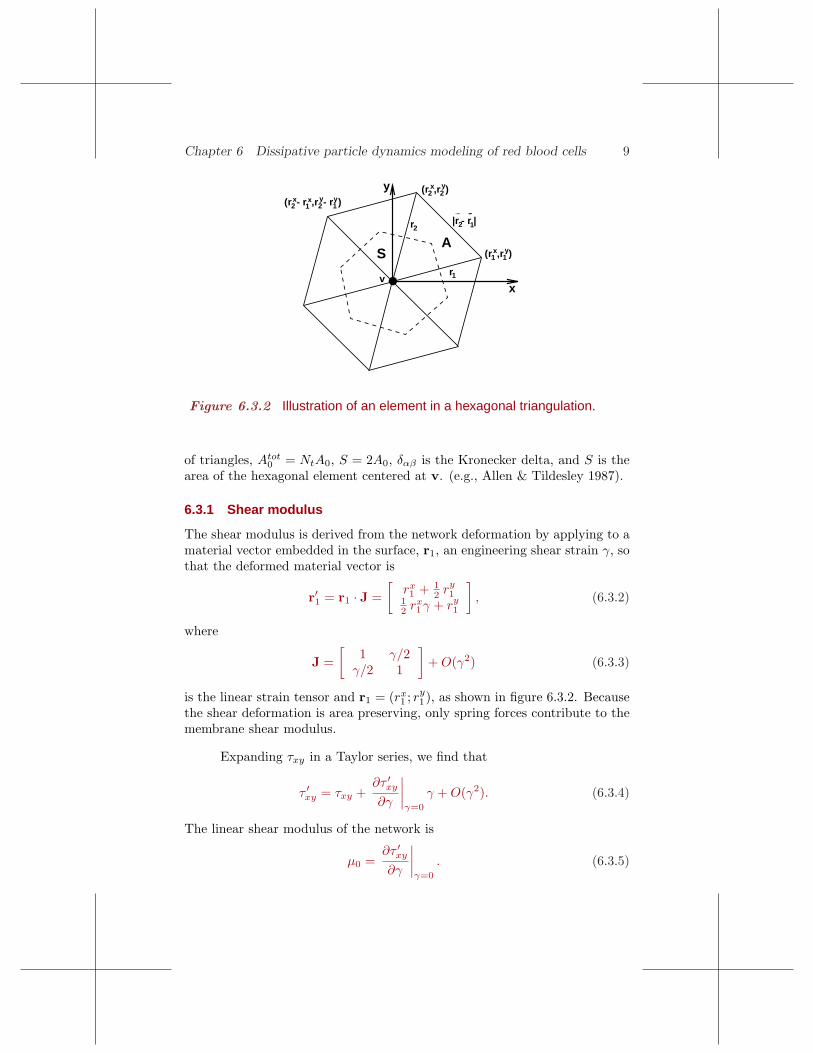
Figure 6.3.2 illustrates an element in a hexagonal network with vertexv placed at the origin of a local Cartesian system. Using the virial theorem,we find that the Cauchy stress tensor at v is

ταβ =− 1

S

[

f(r1)

r1rα1 rβ

1 +f(r2)

r2rα2 rβ

2 +f(|r2 − r1|)|r2 − r1|

(rα2 −rα

1 )(rβ2 −rβ

1 )

]

−(

qCq

Aq+1+

ka(Atot0 − NtA)

Atot0

+kd(A0 − A)

A0

)

δαβ , (6.3.1)

where α and β stand for x or y, f(r) is the spring force, Nt is the total number


(r - r ,r - r )x y(r ,r )x y

x

y

A

x y

r

r

|r - r |

v

S (r ,r )x y

1

2

1

1

2 2

12 12

1

2

Figure 6.3.2 Illustration of an element in a hexagonal triangulation.

of triangles, Atot0 = NtA0, S = 2A0, δαβ is the Kronecker delta, and S is the

area of the hexagonal element centered at v. (e.g., Allen & Tildesley 1987).

6.3.1 Shear modulus

The shear modulus is derived from the network deformation by applying to amaterial vector embedded in the surface, r1, an engineering shear strain γ, sothat the deformed material vector is

r′1 = r1 · J =

[

rx1 + 1

2 ry1

12 rx

1γ + ry1

]

, (6.3.2)

where

J =

[

1 γ/2γ/2 1

]

+ O(γ2) (6.3.3)

is the linear strain tensor and r1 = (rx1 ; ry

1), as shown in figure 6.3.2. Becausethe shear deformation is area preserving, only spring forces contribute to themembrane shear modulus.

Expanding τxy in a Taylor series, we find that

τ ′xy = τxy +

∂τ ′xy

∂γ

∣

∣

∣

∣

γ=0

γ + O(γ2). (6.3.4)

The linear shear modulus of the network is

µ0 =∂τ ′

xy

∂γ

∣

∣

∣

∣

γ=0

. (6.3.5)


For example, differentiating the first term of τxy yields

∂

∂γ

(f(r′1)

r′1rx′

1 ry′

1

)

γ=0=

(∂ f(r1)r1

∂r1

(rx1ry

1)2

r1+

f(r1)r1

2

)

r1=ℓ0. (6.3.6)

Using the vector-product definition of the area of a triangle, we obtain

(rx1ry

1)2 + (rx2ry

2)2 + (rx2 − rx

1 )2(ry2 − ry

1)2 = 2A20. (6.3.7)

The linear shear modulus of the WLC-C and WLC-POW models is

µWLC−C0 =

√3kBT

4pℓmx0

( 3

4(1 − x0)2− 3

4+ 4x0 +

x0

2(1 − x0)3)

(6.3.8)

and

µWLC−POW0 =

√3kBT

4pℓmx0

( x0

2(1 − x0)3− 1

4(1 − x0)2+

1

4

)

+

√3kp(m + 1)

4ℓm+10

.

(6.3.9)

6.3.2 Compression modulus

The linear elastic area compression modulus K is found from the in-planepressure following a small area expansion as

p = −1

2(τxx + τyy) =

3 ℓ

4Af(ℓ) + q

Cq

Aq+1+

(ka + kd)(A0 − A)

A0. (6.3.10)

Defining the compression modulus as

K = − ∂p

∂ log A

∣

∣

∣

A=A0

= −1

2

∂p

∂ log ℓ

∣

∣

∣

ℓ=ℓ0= −1

2

∂p

∂ log x

∣

∣

∣

x=x0

, (6.3.11)

and using equations (6.3.10) and (6.3.11), we obtain

KWLC−C=

√3kBT

4pℓm(1 − x0)2[

(q+1

2) (4x2

0−9x0+6)+1 + 2(1 − x0)

3

1 − x0

]

+ka+kd

(6.3.12)

and

KWLC−POW = 2µWLC−POW0 + ka + kd. (6.3.13)

For q = 1, we find

KWLC−C = 2µWLC−C0 + ka + kd. (6.3.14)


For the nearly constant-area membrane enclosing a red blood cell, the com-pression modulus is much larger than the shear elastic modulus.

The Young modulus and Poisson’s ratio of the two-dimensional sheetare given by

Y = 4Kµ0

K + µ0, ν =

K − µ0

K + µ0. (6.3.15)

As K → ∞, we obtain Y → 4µ0 and ν → 1, as required. To ensure a nearlyconstant area, we set ka + kd ≫ µ0. In practice, the values µ0 = 100 andka+kd = 5000, yield a nearly incompressible membrane with Young’s modulusabout 2% smaller than the asymptotic value 4µ0.

The analytical expressions given in (6.3.15) were verified by numericaltests on a regular two-dimensional sheet of springs. The two-dimensional sheetwas confirmed to be isotropic for small shear strains and stretches, but wasfound to be anisotropic for large deformations (e.g., Fedosov 2010).

6.3.3 Bending rigidity

Helfrich (1973) proposed an expression for the bending energy of the mem-brane of a red blood cell,

Ec =kc

2

∫∫

(C1 + C2 − 2C0)2 dA + kg

∫∫

C1C2 dA, (6.3.16)

where C1 and C2 are the principal curvatures, C0 is the spontaneous curvature,and kc, kg are bending rigidities. The second term on the right-hand sideof(6.3.16) is constant and thus inconsequential for any closed surface.

A relationship between the bending modulus, kb, and the macroscopicmembrane bending rigidity, kc, can be derived for a spherical shell. Figure6.2.1 shows two equilateral triangles with edge length r whose vertices lie ona sphere of radius L. The angle between the triangle normals n1 and n2 isdenoted by φ. In the case of a spherical shell, the total energy in (6.3.16) isfound to be

Ec = 8πkc

(

1 − C0

C1

)2

+ 4πkg = 8πkc

(

1 − L

L0

)2

+ 4πkg, (6.3.17)

where C1 = C2 = 1/L and C0 = 1/L0. In the network model, the energy ofthe triangulated sphere is

VB = Ns kb [1 − cos(φ − φ0)]. (6.3.18)

Expanding cos(φ − φ0) in a Taylor series around φ − φ0 provides us with theleading term

VB =1

2Nskb(φ − φ0)

2 + O(

(φ − φ0)4)

. (6.3.19)


With reference to figure 6.3.2, we find that 2a ≈ φL or φ = r/(√

3L), andφ0 = r/(

√3L0).

For a sphere, A = 4πL2 ≈ NtA0 =√

3Ntr2/4 =

√3Nsr

2/6, andr2/L2 = 8π

√3/Ns. Finally, we obtain

VB=1

2Nskb

( r√3L

− r√3L0

)2=

Nskbr2

6L2

(

1− L

L0

)2=

4πkb√3

(

1− L

L0

)2. (6.3.20)

Equating the macroscopic bending energy Ec to VB for kg = −4kc/3 andC0 = 0, we obtain kb = 2kc/

√3 in agreement with the limit of a continuum

approximation (e.g., Lidmar et al. 2003).

The spontaneous angle φ0 is set according to the total number of verticeson the sphere, Nv. It can be shown that cosφ = 1−1/[6(L2/r2−1/4)] and thenumber of side is Ns = 2Nv − 4. The bending stiffness, kb, and spontaneousangle, φ0, are given by

kb =2√3

kc, φ0 = arccos(

√3(Nv − 2) − 5π√3(Nv − 2) − 3π

)

. (6.3.21)

6.3.4 Membrane viscosity

Since interparticle dissipative interaction is an intrinsic part of the formula-tion, incorporating dissipative and random forces into springs fits naturallyinto the DPD scheme. Straightforward implementation of standard DPD dis-sipative and random interactions expressed by (6.2.1) is insufficient. Thereason is that, when projected onto the connecting vector, the contributionof the inter-particle relative velocity, vij , is negligible for small dissipativecoefficients γ. Large values promote numerical instability.

Best performance is achieved by assigning to each spring a viscous dis-sipation force −γvij , where γ is a scalar coefficient. However, any alterationof the dissipative forces requires a corresponding change in fluctuating forcesconsistent with the fluctuation-dissipation balance to ensure a constant mem-brane temperature, kBT . The general framework of the fluid-particle modelis employed with the following definitions

FDij = −Tij · vij , Tij = A(rij) I + B(rij) eijeij , (6.3.22)

and

FRij dt =

√

2kBT(

A(rij) dWSij

+B(rij)1

3tr[dWij ] I + C(rij) dWA

ij

)

· eij , (6.3.23)


where superscripts R and D stand for “random” and “dissipative”, I is theidentity matrix, tr[dWij ] is the trace of a random matrix of independentWiener increments dWij whose symmetric and anti-symmetric parts are de-noted with superscripts S and A, and

dWSij ≡ dWS

ij −1

3tr[dWS

ij ] I (6.3.24)

is the traceless symmetric part (e.g., Espanol 1998) . The scalar weight func-tions A(r), B(r), A(r), B(r), and C(r) are related by

A(r)=1

2

[

A2(r)+C2(r)]

,

B(r)=1

2

[

A2(r)−C2(r)]

+1

3

[

B2(r)−A2(r)]

. (6.3.25)

The standard forms of the dissipative and random forces are recovered bysetting A(r) = C(r) = 0 and B(r) = γ. We employ spatially constant weightfunctions A(r) = γT , B(r) = γC , and C(r) = 0. where γT and γC aredissipative coefficients. Accordingly,

Tij = γT I + γCeijeij (6.3.26)

and the dissipative interaction force becomes

FDij = −

(

γT 1 + γCeijeij

)

· vij = −γT vij − γC(vij · eij) eij . (6.3.27)

The first term on the right-hand side provides the main viscous contribution.The second term is identical in form to the central dissipative force of stan-dard DPD introduced in section 6.2.1. To satisfy the fluctuation-dissipationbalance, the following random interaction force ensuring 3γC > γT is used,

FRijdt = (2kBT )1/2

(

(2γT )1/2dWSij + (3γC − γT )1/2 1

3tr[dWij ] I

)

· eij .

(6.3.28)

These stipulations for the dissipative and the random forces in combinationwith an elastic spring constitute a mesoscopic viscoelastic spring.

To relate the membrane shear viscosity, ηm, to the model dissipativeparameters γT and γC , an element of the hexagonal network shown in figure6.3.2 is subjected to a constant shear rate, γ. The shear stress τxy at shorttimes can be approximated from the contribution of the dissipative force in(6.3.27),

τxy = − 1

2A0

[

γT γ(

(r1y)2 + (r2

y)2 + (r2y − r1

y)2)

+γC γ

l20

(

(r1xr1

y)2 + (r2xr2

y)2 + (r2x − r1

x)2(r2y − r1

y)2)]

(6.3.29)

= γ√

3 (γT +1

4γC ).


Figure 6.4.1 A slice through a sample equilibrium simulation. Red parti-cles are membrane vertices, blue particles represent the external fluid,and green particles represent the internal fluid. (Color coded in theelectronic file.)

The membrane viscosity is given by

ηm =τxy

γ=

√3 (γT +

1

4γC). (6.3.30)

As stated in section 6.2.1, simulations with the central viscous forcealone corresponding to γT = 0 indicate that γT accounts for the largest por-tion of the membrane dissipation. Accordingly, the numerical results areinsensitive to the value of γC . Since large values lead to numerical instability,γC is set to its minimum value, 1

3 γT , in the simulations.

6.4 Membrane-solvent interfacial conditions

The cell membrane encloses a viscous fluid and is surrounded by a liquidsolvent. Figure 6.4.1 shows a snapshot of a simulation at equilibrium. wherered particles are membrane vertices, blue particles represent the external fluid,and green particles represent the internal fluid. To prevent mixing of theinternal and external fluids, we require impenetrability and enforce adherenceor no-slip implemented by pairwise interactions between fluid particles andmembrane nodes.

Bounce-back reflection of fluid particles at the triangular plaquettessatisfies membrane impenetrability and better enforces no-slip compared tospecular reflection. However, bounce-back reflection alone does not guaran-tee no-slip, nor does it suppress large unphysical density fluctuations. Fluid


particles whose centers are located at a distance less than a cutoff radius, rc,require special treatment to account for interactions in the spherical cap lyingoutside the fluid domain. In practice, this necessitates the DPD dissipativeforce coefficient between fluid particles and membrane vertices to be properlyset (e.g., Fedosov 2010).

The continuum linear shear flow over a flat plate is used to determinethe dissipative force coefficient γ for the fluid in the vicinity of the membrane.For the continuum, the total shear force on area A of the plate is Aηγ, whereη is the fluid viscosity and γ is the local shear-rate. To mimic the membranesurface, wall particles are distributed over the plate to match the configurationof the cell network model. The force on a single wall particle in this systemexerted by the surrounding fluid under shear can be expressed as

Fv =

∫∫∫

Vh

n g(r)FD dV, (6.4.1)

where FD is the DPD dissipative force between fluid and wall particles, nis the fluid number density, g(r) is the radial distribution function of fluidparticles relative to the wall particles, and Vh is the half-sphere volume offluid above the plate. Thus, the total shear force on the area A is equal toNAFv, where NA is the number of plate particles residing in the area A. Whenconservative interactions between fluid particles and the membrane verticesare neglected, the radial distribution function simplifies to g(r) = 1.

Setting NAFv = Aηγ yields an expression for the dissipative force co-efficient γ in terms of the fluid density and viscosity and the wall density,NA/A. Near a wall where the half-sphere lies within the range of the linearwall shear flow, the shear rate cancels out. This formulation has been veri-fied to enforce satisfactory no-slip boundary conditions without unacceptablewall density fluctuations for the linear shear flow over a flat plate, and is anexcellent approximation for no-slip at the membrane surface.

6.5 Numerical and physical scaling

The dimensionless constants and variables in the DPD model must be scaledwith physical units. The characteristic length scale rM is based on the cell di-ameter at equilibrium, DM

0 , where [DM0 ] = rM and the superscript M denotes

model units. The equilibrium spring length, ℓM0 , appears to be too small a

scale since the cell dimensions depend generally on the relative volume-to-arearatio. For example, although a red blood cell and a spherical capsule withthe same volume may have different surface areas, but they may still havethe same ℓM

0 after triangulation. If the volume-to-area ratio is fixed, DM0 is

proportional to ℓM0 .


The length scale adopted in the present work is

rM =DP

0

DM0

[m], (6.5.1)

where the superscript P denotes physical units, and [m] stands for meters.Young’s modulus is used as an additional scaling parameter. An energy unitscale can be derived by equating the model and physical Young’s moduli,

Y M (kBT )M

(rM )2= Y P (kBT )P

m2, (6.5.2)

yielding the model energy scale,

(kBT )M =Y P

Y M

(rM )2

m2(kBT )P =

Y P

Y M

(

DP0

DM0

)2

(kBT )P . (6.5.3)

Once the model energy unit is defined, the membrane bending rigidity can beexpressed in energy units. With the above length and energy scales, the forcescale for membrane stretching is given by

NM =(kBT )M

rM=

Y P

Y M

DP0

DM0

(kBT )P

m=

Y P

Y M

DP0

DM0

NP . (6.5.4)

Membrane rheology and dynamics require a time scale in addition tothe scales previously defined. A general model time scale is defined as

τ =tPitMi

s =

(

DP0

DM0

ηPo

ηMo

Y M0

Y P0

)α

s, (6.5.5)

where ηo is the exterior fluid viscosity and α is a chosen scaling exponentsimilar to the power-law exponent in rheology.

6.6 Membrane mechanics

The mechanical properties of cell membranes are typically measured by defor-mation experiments using either micropipette aspiration techniques or opticaltweezers (e.g., Evans 1983, Discher et al. 1994, Henon et al. 1999, Suresh etal. 2005). It has been estimated that the shear modulus µ0 of a healthy RBClies in the range 2 – 12 µN/m, and the bending rigidity kc lies in the range1 × 10−19 – 7 × 10−19 J corresponding to 25–171 kBT at room temperature23◦C.

To set the mechanical properties of the network model, triangulationof the cell shape described by equation (6.2.15) is first performed yielding an


equilibrium spring length

ℓ0 =1

Ns

Ns∑

i=1

ℓi0. (6.6.1)

A shear modulus of a healthy cell provides us with a scaling base, µ0 = µM0 .

The WLC spring model requires setting the maximum extension length, ℓMm .

However, it is more convenient to set the ratio x0 = ℓM0 /ℓM

m governing thecell nonlinear response at large deformation. The ratio x0 is fixed at 2.2 in allsimulations (e.g., Fedosov 2010).

Necessary model parameters can be calculated from (6.3.9) for givenvalues of ℓM

0 , µM0 , and x0, thereby circumventing manual adjustment. The

calculation of the areal compression modulus KM and Young’s modulus Y M

follows from equations (6.3.13, 6.3.15). for specified area constraint parame-ters ka and kd. In the simulations, we use µM

0 = 100, ka = 4900, kd = 100, andkv = 5000. We note that the global areal compression and volume constraintsare strong, while the local area constraint is weak. The bending rigidity kc

is set to 58(kBT )M corresponding to physical units 2.4 × 10−19 J at roomtemperature. The exponent m in relation (6.2.8) is set to 2.

6.6.1 Equilibrium shape and the stress-free model

After initial setup, an equilibrium simulation is run to confirm that the cellretains the biconcave shape. Figure 6.6.1(a) shows an equilibrated shape com-puted with the WLC-C and the WLC-POW model using typical red bloodcell parameters. If all springs have the same equilibrium length, a networkon a non-developable surface cannot be constructed with triangles having thesame edge lengths. Consequently, the cell surface would necessarily developlocal bumps manifested as stress anomalies at the level of a continuum. Infact, the potential energy relaxation performed during the triangulation pro-cess produces triangles with a narrow distribution of spring lengths arounda specified equilibrium value. Accordingly, a network constructed withoutannealing implemented by further energy relaxation of the equilibrium shapewould still display pronounced bumps and would fail to relax to an equilibriumstress-free axisymmetric shape.

The relaxed cell shape is affected by the ratio of the membrane modu-lus of elasticity to the bending rigidity expressed by the Foppl-von Karmannumber

κ =Y0R

20

kc, (6.6.2)

where R0 =√

πA0/4. Figure 6.6.1 (b) displays an equilibrated shape com-puted with the WLC-C or WLC-POW model. The bending rigidity is ten


(a) (b) (c)

Figure 6.6.1 Equilibrium shape of a cell computed with the WLC-C orWLC-POW model for (a) kc = 2.4 × 10−19 J and (b) kc = 2.4 × 10−20 J.(c). Equilibrium shape with the WLC-POW stress-free model for kc =2.4 × 10−20 J.

times lower than that of the red blood cell membrane, kc = 2.4 × 10−19 J.Membrane stress artifacts are significantly pronounced under these conditions.

Shape regularization

A stress-free shape eliminating membrane stress anomalies is obtainedby computational annealing. For each spring, the equilibrium spring length ℓi

0

is adjusted to be the edge length after triangulation, while the ratio x0 is keptconstant at 2.2, for i = 1, . . . , Ns. The maximum spring extension is then setindividually to ℓi

m = li0 × x0. The initial cell network defines local areas foreach triangular plaquette, Aj

0, for j = 1, . . . , Nt. The total cell surface area,

Atot0 =

Nt∑

j=1

Aj0, (6.6.3)

and the total cell volume, V tot0 , are calculated from the triangulation. After

this adjustment, a new network that is virtually free of irregularities appears.A stretching test along a diameter repeated along several diameters is usedto verify that the red cell model behaves like a transversely isotropic body, asdiscussed in the next section.

The annealing process disqualifies the WLC-C model. The reason isthat the assumed isotropic in-plane area-expansion potential expressed bythe last term in (6.2.7) is not able to accommodate individual equilibriumspring lengths for each triangle side. Because the POW potential is defined interms of spring length, it is endowed with the necessary degrees of freedom forequilibrium length adjustment. The individual spring parameters pi and ki

s ofthe WLC-POW model are recalculated based on ℓi

0, ℓim, µM

0 using (6.3.9) in


(a) (b)

DT

DA

N

N

-

x

x

xx

xx x x x x x x x x x x x x

x x x x x x x x x x x x x x x x x

force (pN)

diam

eter

(m

)

0 50 100 150 2000

2

4

6

8

10

12

14

16

18

20ExperimentNv = 100Nv = 500Nv = 3000Nv = 9128Nv = 27344x

µ

D

D

A

T

Figure 6.6.2 (a) Schematic illustration of cell deformation. (b) Stretchingresponse with the WLC-POW stress-free model for different coarse-graining levels or number of vertices Nv in the network representation.The diamonds represent experimental results by Suresh et al. (2005).

conjunction with the relation fWLC = fPOW for the given spring equilibriumlength.

Figure 6.6.1(c) shows an equilibrium shape computed with the WLC-POW stress-free model for bending rigidity kc = 2.4×10−20 J. Because mem-brane stress artifacts are eliminated, arbitrary surface networks can be em-ployed even for small flexural stiffness. However, if the generated networkdeparts too much from a regular hexagonal triangulation, the analytic for-mulas used to estimate the network macroscopic properties are no longer bereliable.

Stretching test

The reconstructed cell is subjected to stretching analogous to that im-posed on cells in optical tweezers experiments (Suresh et al. 2005). A stretch-ing force FP

s up to 200 pN is applied to the outermost N+ = ǫNv verticeswith the largest x coordinates in the positive x direction, and to the outer-most N− = N+ vertices with the smallest x coordinates in the negative xdirection, as shown in figure 6.6.2(a). The vertex fraction ǫ is set to 0.02,corresponding to contact diameter of an attached silica bead dc = 2 µm usedin the experiments.

For each external force, the cell is allowed to relax to an equilibriumstretched state. The axial diameter, DA, defined as the maximum distance


between the sets of points N+ and N−, and the transverse diameter, DT , de-fined as the maximum distance between two points from the set of all verticesprojected on a plane perpendicular to the axial diameter, are averaged duringa specified simulation time. Results presented in figure 6.6.2(b) are in goodagreement with experimental data for all levels of coarse graining. Noticeablediscrepancies for the transverse diameter are observed inside the error barsdue to experimental error. The optical measurements were performed from asingle observation angle. Numerical simulations show that stretched cells mayrotate in the yz plane. Consequently, measurements from a single observationangle are likely to underpredict the maximum transverse diameter.

6.7 Membrane rheology from twisting torque cytometry

Early measurements of cell relaxation time employed a micropipette techniqueto study cell extension and recovery (e.g., Hochmuth et al. 1979). The relax-ation time extracted from an exponential fit of cell recovery after deformationis on the order of 0.1 s. However, since the deformation is inherently nonuni-form in these experiments, it is doubtful that the global technique produces anaccurate characteristic membrane time scale (e.g., Yoon et al. 2008, Fedosov2010).

In recent experiments, Puig-de-Morales-Marinkovic et al. (2007) ap-plied optical magnetic twisting cytometry (OMTC) to infer a dynamic com-plex modulus of the cell membrane. In this procedure, the cell membraneresponse is measured locally by observing the motion of an attached ferro-magnetic microbead driven by an oscillating magnetic field. The experimentshave confirmed that the membrane is a viscoelastic material. Our viscoelas-tic membrane model will be tested against the results of optical magnetictwisting cytometry. The numerical simulations emulate the aforementionedexperiments where the motion of a microbead attached to the flat side of thebiconcave cell due an oscillating torque is studied, as shown in figure 6.7.1(a).The data allow us to infer membrane properties such as the complex modulus.

In the numerical model, the microbead is represented by a set of verticesdeployed on a rigid sphere. A group of cell vertices near the bottom of themicrobead simulates the area of attachment. The torque on the microbead isapplied only to the bead vertices. Figure 6.7.1(b) presents a typical response toan oscillating torque. The bead motion, monitored by the displacement of thecenter of mass, oscillates with the applied torque frequency. The oscillationis shifted by a phase angle, φ, that depends on the applied frequency. In thecase of a purely elastic material and in the absence of inertia, the phase angleφ would be zero zero for any torque frequency.

The linear complex modulus of a viscoelastic material can be extracted


(a) (b)

displacement

oscillating torque on the attached bead

displacement

0 2 4 6 8 10 12−0.3

−0.2

−0.1

0

0.1

0.2

0.3

Dimensionless time − tω

Tor

que

per

unit

volu

me

(Pa)

0 2 4 6 8 10 12−300

−200

−100

0

100

200

300

Dis

plac

emen

t (nm

)

ω = 1.9 Hz

Torque Displacement

φ

Figure 6.7.1 (a) Illustration of the numerical setup of the twisting torquecytometry. (b) Response of an attached microbead subject to an oscil-lating torque exerted on the bead.

from the phase angle and torque frequency using the relations

g′(ω) =∆T

∆dcos φ, g′′(ω) =

∆T

∆dsinφ, (6.7.1)

where g′(ω) and g′′(ω) are two-dimensional storage and loss moduli and ∆Tand ∆d are the torque and bead displacement amplitudes. In the absence ofinertia, the phase angle φ ranges between 0 and π/2.

Figure 6.7.2 compares the computed complex modulus with experi-mental data by Puig-de-Morales-Marinkovic et al. (2007). Good agreementis found for bending rigidity kc = 4.8 × 10−19 J and membrane viscosityηm = 0.022 Pa s. Numerical twisting cytometry suggests that the storagemodulus behaves as

g′(ω) ∼ (kcY0)0.65. (6.7.2)

Since the Young modulus of healthy cells is fixed by the cell stretching test,figure 6.7.2 essentially illustrates the dependence of g′ on the membrane bend-ing rigidity. To ensure good agreement with experiments, the bending rigidityof a healthy cell must be in the range 4 to 5 × 10−19 J, which is twice thewidely adopted value, kc = 2.4 × 10−19 J.

For small displacements, the loss modulus g′′ depends mainly on thesurface viscosity and is insensitive to the membrane’s elastic properties. Thesimulated loss modulus follows a power law in frequency with exponent α =


10−2

10−1

100

101

102

103

104

10−5

10−4

10−3

10−2

10−1

Frequency (Hz)

g’ a

nd g

’’ (P

a/nm

)

g’ − OMTCg’’ − OMTCg’ −g’ −g’’ −g’’ −g’’ −

0 5 10−2

−1.5

−1

−0.5

0

0.5

1

1.5

2

Dimensionless time − tω

Tor

que

per

unit

volu

me

(Pa)

0 5 10−300

−200

−100

0

100

200

300

Dis

plac

emen

t (nm

)

kc= 2.4×10−19 J

kc= 4.8×10−19 J

ηm

= 0.01 Pa⋅sη

m= 0.022 Pa⋅s

ηm

= 0.04 Pa⋅sω0.85

ω0.65

ω = 94.5 HzDisplacement

φ>π/2

Torque

Figure 6.7.2 Graphs of the functions g′ and g′′ obtained from simulationswith different membrane viscosities and bending rigidities. The numer-ical results are compared with experimental data by Puig-de-Morales-Marinkovic et al. (2007). The inset illustrates the effect of inertia forhigh frequencies of the driving torque.

0.85 to be used in (6.5.5). In the experiments, the exponent is approximately0.75. The agreement is fair in view of fitting errors in only two frequencydecades in simulation and experiment. The inset in figure 6.7.2 shows thatinertial effects affect g′ at high frequencies. Decreasing the bead mass wouldallow us to obtain rheological data for higher torque frequencies, but thecomputational cost is high since a small time step is required. When the lossmodulus dominates the storage modulus, the bead-displacement amplitudeat fixed torque amplitude is extremely small and hard to measure in thelaboratory. However, bead displacements in simulations can be successfullydetected on a scale of several nanometers.

6.8 Deformation in shear flow

Experimental observations have shown that red blood cells tumble at low shearrates and exhibit a tank-treading motion at high shear rates (e.g., Tran-Son-Tay et al. 1984, Fischer 2004, 2007, Abkarian et al. 2007). Fischer (2004)attributed this behavior to a minimum elastic energy state of the cell mem-brane. Cells can be made to tank-tread in the laboratory for several hours.


When the flow is stopped, the cells relax to the original biconcave shape whereattached microbeads recover their original relative position. It appears thattank-treading is possible only when a certain elastic energy barrier has beensurpassed. Theoretical analyses have considered ellipsoidal cell models tank-treading along a fixed ellipsoidal path (e.g., Abkarian et al. 2007, Skotheim& Secomb 2007). Our simulations show that the dynamics depends on themembrane shear modulus, shear rate, and viscosity ratio λ = (ηi + ηm)/ηo,where ηi, ηm, and ηo are the interior, membrane, and outer fluid viscosities.

For viscosity ratio λ < 3, the theory predicts tumbling at low shearrates and tank-treading motion at high shear rates (e.g., Skotheim & Secomb2007). The cells exhibit an unstable behavior in a narrow intermittent regionaround the tumbling-to-tank-treading transition where tumbling can be fol-lowed by tank-treading and vice versa. For λ > 3, stable tank-treading doesnot necessarily arise. Red blood cells with viscosity ratio λ > 3 have beenobserved to tank-tread while exhibiting a swinging motion with a certain fre-quency and amplitude about an average tank-treading axis. The reliability ofthe theoretical predictions will be judged by comparison with the results ofour simulations.

In the first simulation, a cell is suspended in a linear shear flow betweentwo parallel walls. The viscosities of the external solvent and internal cytosolfluid are set to ηo = ηi = 0.005 Pa s. Consistent with results of twisting torquecytometry, the membrane viscosity is set to ηm = 0.022 Pa s. Figure 6.8.1presents information on the cell tumbling and tank-treading frequencies underdifferent conditions. Experimental observations by Tran-Son-Tay et al. (1984)and Fischer (2007) are included for comparison.

In the case of a purely elastic membrane with or without inner solvent(circles and squares), the numerical results significantly overpredict the tank-treading frequency compared with experimental measurements. The internalsolvent viscosity could be further increased to improve agreement with ex-perimental data. However, since the cytosol is a hemoglobin solution witha well-defined viscosity of about 0.005 Pa s, excess viscous dissipation mustoccur inside the membrane (e.g., Cokelet and Meiselman 1968). The dataplotted with triangles in figure 6.8.1 show good agreement with experimentaldata for increased membrane viscosity.

The tumbling frequency is nearly independent of the medium viscosi-ties. Increasing the viscosity of the internal fluid or raising the membraneviscosity slightly shifts the tumbling-to-treading threshold into higher shearrates through an intermittent regime. We estimate that the tank-treadingenergy barrier of a cell is approximately Ec = 3 to 3.5 × 10−17 J . In a theo-retical model proposed by Skotheim & Secomb (2007), the energy barrier was


Fre

quen

cy(r

ad/s

)

0 50 100 150 2000

20

40

60

80

all viscositiesTran-Son-Tay et al. (1984)Fischer (2007)

γ (s )-1

Tum

blin

g

Tan

k-tre

adin

g

Inte

rmitt

ent

ηηi

m= 0m= = 0η

Figure 6.8.1 Tumbling and tank-treading frequency of a RBC in shearflow for ηo = 0.005 Pa s, ηi = ηm = 0 (circles); ηo = ηi = 0.005 Pas, ηm = 0 (squares); ηo = ηi = 0.005 Pa s, ηm = 0.022 Pa s (triangles).

set to Ec = 10−17 J to ensure agreement with experimental data. Membranedeformation during tank treading is indicated by an increase in the elasticenergy difference with increasing shear rate to within about 20% of Ec.

An intermittent regime is observed with respect to the shear rate inall cases. Consistent with the experiments, the width of the transition zonebroadens as the membrane viscosity increases. Similar results regarding inter-mittency were reported by Kessler et al. (2008). for viscoelastic vesicles. Weconclude that theoretical predictions of cell dynamics in shear flow are qual-itative correct at best due to the assumption of ellipsoidal shape and fixedellipsoidal tank-treading path. Experiments by Abkarian et al. (2007) haveshown and the present simulations have confirmed that the cell deforms alongthe tank-treading axis with strains of order 0.1 − 0.15.

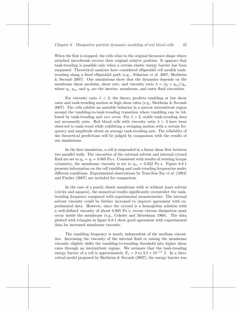
Cell deformation in shear flow depends on the ratio of the membraneelastic to bending modulus, expressed by the Foppl-von Karman number κdefined in (6.6.2). Figures 6.8.2 (a) and (b) show several snapshots of tumblingand tank-treading cells with bending rigidity set to ten times that commonlyused for red blood cells, kc = 2.4 × 10−18 J, corresponding to Foppl-vonKarman number κ = 85. Tumbling to tank-treading transition occurs at shear


(a) γ = 8 s -1

γ = 16 s -1

(b) γ = 32 s -1

γ = 190 s -1

Figure 6.8.2 Snapshots of (a) a tumbling and (b) a tank-treading cell atdifferent shear rates, for viscosities ηo = ηi = 0.005 Pa s, ηm = 0.022 Pas, bending rigidity kc = 2.4 × 10−18 J, and Foppl-von Karman numberκ = 85. Blue particles are added as tracers during post-processing forvisual clarity. (Color in the electronic file.)

rates 20–25 s−1. The results show negligible deformation during tumbling andsmall deformation during tank-treading following the transition.

Figure 6.8.3 presents analogous results for tumbling and tank-treadingcells with bending rigidity kc = 2.4 × 10−19 J corresponding to κ = 850.Significant shape deformation is observed during tumbling and tank-treading.However, the frequency of the motion is hardly changed from that corre-sponding to κ = 85. Since the discrete network cannot adequately capturethe membrane bending on length scales comparable to the element size, afurther decrease of the bending rigidity results in buckling. To screen outthe effect of the membrane discretization, simulations were performed withNv = 1000 and 3000 membrane network vertices and similar results were


(a) γ = 8 s -1

γ = 16 s -1

(b) γ = 32 s -1

γ = 190 s-1

Figure 6.8.3 Snapshots of (a) a tumbling and (b) a tank-treading cell atdifferent shear rates for viscosity ηo = ηi = 0.005 Pa s, ηm = 0.022 Pas, bending rigidity kc = 2.4 × 10−19 J, and Foppl-von Karman numberκ = 850. Blue particles are added as tracers during post-processing forvisual clarity. (Color in the electronic file.)

obtained for corresponding Foppl-von Karman numbers.

The simulations suggest that the membrane bending rigidity is severaltimes larger than the widely accepted value kc = 2.4 × 10−19 J. Simulationsof twisting torque cytometry presented previously in this chapter corroboratethis assertion. An increase in the membrane shear modulus raises the Foppl-von Karman number and the tank-treading energy barrier Ec, and hence alsoshifts the tumbling-to-tank-treading transition to higher shear rates.

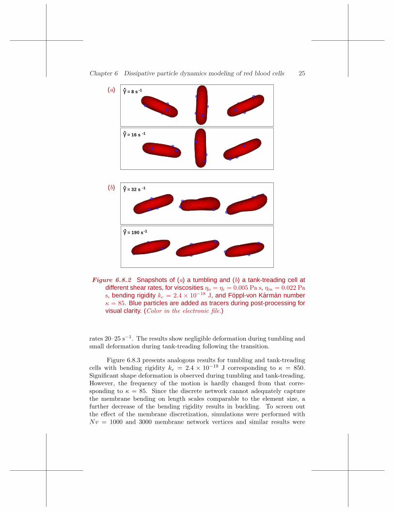
We have seen that a cell oscillates or swings around tank-treading axeswith a certain frequency and amplitude, as shown in figures 6.8.2 and 3.Figure 6.8.4 presents graphs of the average tank-treading angle and swinging


Sw

ingi

ngan

gle

and

ampl

itude

(deg

rees

)

0 50 100 150 2000

5

10

15

20

25

30

35

40

γ (s )-1

average angle

= 0ηm

amplitude

ηm

= = 0ηi

all viscosities

Figure 6.8.4 Graphs of the swinging average angle in degrees (filledsymbols) and amplitude (open symbols) for (a) ηo = 0.005 Pa s andηi = ηm = 0 (circles); (b) ηo = ηi = 0.005 Pa s and ηm = 0 (squares);(c) ηo = ηi = 0.005 Pa s and ηm = 0.022 Pa s (triangles).

amplitude. The numerical results are consistent with experimental data byAbkarian et al. (2007). The average swinging angle is larger for a purelyelastic membrane without inner cytosol. The inclination angle is independentof the internal fluid and membrane viscosities and the swinging amplitude isinsensitive to the fluid and membrane properties. The swinging frequency isexactly twice the tank-treading frequency.

6.9 Tube flow

The mean velocity of Poiseuille flow in a circular tube is defined as

v =1

S

∫∫

v(r) dS, (6.9.1)

where S is the cross-sectional area and v(r) is the axial velocity. For a New-tonian fluid, v = vc/2, where vc is the centerline velocity.

At low flow rates, a cell suspended in tube flow retains its bicon-cave shape. As the driving pressure gradient increases, the cell obtains theparachute-like shape shown in figure 6.9.1 for a tube with diameter 9µm, in


Figure 6.9.1 Parachute shape of a cell suspended in Poiseuille flowthrough a 9µm diameter tube.

agreement with experimental observations (e.g., Tsukada et al. 2001). Toidentify the biconcave-to-parachute transition, we compute the gyration ten-sor

Gmn =1

Nv

∑

i

(rim − rC

m)(rin − rC

n ), (6.9.2)

where ri are the membrane vertex coordinates, rC is the membrane centerof mass, and m,n stand for x, y, or z. (e.g., Mattice & Suter 1994). Theeigenvalues of the gyration tensor allow us to accurately characterize the cellshape. For the equilibrium biconcave shape, the gyration tensor has two largeeigenvalues corresponding to the midplane of the biconcave disk, and onesmall eigenvalues corresponding to the disk thickness. At the biconcave-to-parachute transition, the small eigenvalue increases indicating that the cellelongates along the tube axes.

Figure 6.9.2 illustrates the dependence of the axial eigenvalue on themean flow velocity for different membrane bending rigidities and shear mod-uli. The dashed line describes the biconcave-to-parachute transition. Forhealthy cells, the transition occurs at a mean velocity of about 65 µm/s. Thetransition occurs at larger bending rigidity or membrane shear modulus at


(a) (b)sh

ifted

eige

nva

lue

ofth

egy

ratio

nte

nsor

0 200 400 600 8000

0.2

0.4

0.6

µU ( m/s)

transition to parachute

k = 2.4e-19 Jk = 1.2e-18 Jk = 2.4e-18 J

c

c

c

shift

edei

gen

valu

eof

the

gyra

tion

tens

or

0 200 400 600 8000

0.2

0.4

0.6

U ( m/s)µ

transition to parachute

µ 0µ 0

µ 0= 6.3e-6 N/m

= 63e-6 N/m= 18.9e-6 N/m

Figure 6.9.2 Excess axial eigenvalue of the gyration tensor above thatfor a biconcave disk for (a) different bending rigidities and (b) differentmembrane shear moduli. The cell volume fraction is C = 0.05.

stronger flows. The critical mean velocity changes almost linearly with thebending rigidity, kc, and shear modulus, µ0. These results are consistent withnumerical simulations by Noguchi & Gompper (2005). Stiffer capsules suffersmaller elongation along at the same mean velocity. The results in figure 6.9.2corroborate the notion that stiffer cells exhibit stronger resistance to flow.

The relative apparent viscosity of the suspension is defined as

λapp =ηapp

ηo, ηapp =

nfR20

8u, (6.9.3)

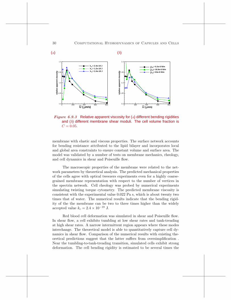
where n is the cell number density, f is the force exerted on each cell, R0 is thetube radius, ηo is the solvent viscosity, and u is the bulk velocity calculatedusing equation (6.9.1). The product nf is the streamwise pressure gradient,∆P/L, where L is the tube length. Figure 6.9.3 reveals a slight increase in theapparent viscosity with cell stiffening due to increased flow resistance. Theeffect is small even for a tenfold increase in the membrane elastic modulusdue to the low cell concentration, C = 0.05. A stronger effect is expected atat higher volume fractions.

6.10 Summary

We have presented a mesoscopic model of red blood cells implemented by thedissipative particle dynamics (DPD) method. The spectrin cytoskeleton isrepresented by a network of interconnected viscoelastic springs comprising a


(a) (b)re

lativ

eap

pare

ntvi

scos

ity

0 200 400 600 8001.2

1.25

1.3

1.35

1.4

µU ( m/s)

c

ck = 2.4e-19 Jk = 1.2e-18 Jk = 2.4e-18 J

c

rela

tive

appa

rent

visc

osity

0 200 400 600 8001.2

1.25

1.3

1.35

1.4

U ( m/s)µ

µµµ

0

0

0

= 6.3e-6 N/m

= 18.9e-6 N/m= 63e-6 N/m

Figure 6.9.3 Relative apparent viscosity for (a) different bending rigiditiesand (b) different membrane shear moduli. The cell volume fraction isC = 0.05.

membrane with elastic and viscous properties. The surface network accountsfor bending resistance attributed to the lipid bilayer and incorporates localand global area constraints to ensure constant volume and surface area. Themodel was validated by a number of tests on membrane mechanics, rheology,and cell dynamics in shear and Poiseuille flow.

The macroscopic properties of the membrane were related to the net-work parameters by theoretical analysis. The predicted mechanical propertiesof the cells agree with optical tweezers experiments even for a highly coarse-grained membrane representation with respect to the number of vertices inthe spectrin network. Cell rheology was probed by numerical experimentssimulating twisting torque cytometry. The predicted membrane viscosity isconsistent with the experimental value 0.022 Pa s, which is about twenty twotimes that of water. The numerical results indicate that the bending rigid-ity of the the membrane can be two to three times higher than the widelyaccepted value kc = 2.4 × 10−19 J.

Red blood cell deformation was simulated in shear and Poiseuille flow.In shear flow, a cell exhibits tumbling at low shear rates and tank-treadingat high shear rates. A narrow intermittent region appears where these modesinterchange. The theoretical model is able to quantitatively capture cell dy-namics in shear flow. Comparison of the numerical results with existing the-oretical predictions suggest that the latter suffers from oversimplification .Near the tumbling-to-tank-treading transition, simulated cells exhibit strongdeformation. The cell bending rigidity is estimated to be several times the


accepted value of kc = 2.4 × 10−19 J. Further experimental data on cell de-formations around the tumbling-to-tank-treading transition could confirm thecomplex dynamics observed in the simulations. Simulations of cell motion inPoiseuille flow through a 9 µm diameter tube demonstrated a transition to aparachute shape at a mean velocity of about 65 µm/s. The threshold occursat higher mean velocities for stiffer cells with a higher bending rigidity orshear modulus.

Most of the current cell models assume that the cell membrane is purelyelastic. The simulations described in this chapter show that membrane viscos-ity is essential for capturing single cell rheology and dynamics. The presentedmodel is general enough to be used with other simulation methods, includ-ing Lattice-Boltzmann, Brownian dynamics, the immersed-boundary method,and multiparticle collision dynamics.

Acknowledgement

This work was supported by the NSF grant CBET-0852948 and by the NIHgrant R01HL094270. Computations were performed at the NSF NICS facility.

Appendix

The modeled membrane is described by the potential energy V ({xi})given in (6.2.6)) with contributions defined in (6.2.7) – (6.2.13). Nodal forcescorresponding to these energies are derived according to equation (6.2.14) andthen divided into three parts: two-point interactions mediated by springs de-fined in (6.2.8) and 6.2.9), three-point interactions representing stored elasticenergy and mediating area and volume conservation constraints according to(6.2.7), (6.2.12), and (6.2.13), and four-point interactions implementing flex-ural stiffness between adjacent faces.

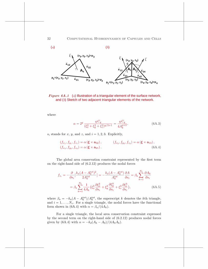
Figure 6A.1(a) shows a sample triangular element of a membrane net-work. We introduce the distance matrix aij = pi − pj , where i and j takethe values 1, 2, and 3, and the normal vector ξ = a21 × a31. The area of thetriangle is

Ak =1

2|ξ| =

1

2(ξ2

x + ξ2y + ξ2

z)1/2. (6A.1)

The stored elastic energy for a single triangle generates the following nodalforces according to (6.2.7),

fsi=−∂ (Cq/A

qk)

∂si=α

(

ξx∂ξx

∂si+ ξy

∂ξy

∂si+ ξz

∂ξz

∂si

)

, (6A.2)


(a) (b)

a21p =(x , y , z )1 1 1 (x , y , z )=p2 2 2

(x , y , z )=p3 3 3ξ

a

kA

a13

3

21

32

a21

p =(x , y , z )1 1 1

(x , y , z )2 2(x , y , z )=p4 4 4

ζ

a

2Aa13

42

1

42

(x , y , z )3 3 3

A1

ξ

θ

a34

Figure 6A.1 (a) Illustration of a triangular element of the surface network,and (b) Sketch of two adjacent triangular elements of the network.

where

α = 2q q Cq

(ξ2x + ξ2

y + ξ2z)q/2+1

=q Cq

4Aq+2k

, (6A.3)

si stands for x, y, and z, and i = 1, 2, 3. Explicitly,

(fx1, fy1

, fz1) = α (ξ × a32) , (fx2

, fy2, fz2

) = α (ξ × a13) ,

(fx3, fy3

, fz3) = α (ξ × a21) . (6A.4)

The global area conservation constraint represented by the first termon the right-hand side of (6.2.12) produces the nodal forces

fsi= − ∂

∂si[ka(A − Atot

0 )2

2Atot0

] = −ka(A − Atot0 )

Atot0

∂A

∂si= βa

Nt∑

k=1

∂Ak

∂si

= βa

Nt∑

k=1

1

4Ak

(

ξkx

∂ξkx

∂si+ ξk

y

∂ξky

∂si+ ξk

z

∂ξkz

∂si

)

, (6A.5)

where βa = −ka(A − Atot0 )/Atot

0 , the superscript k denotes the kth triangle,and i = 1, . . . , Nv. For a single triangle, the nodal forces have the functionalform shown in (6A.4) with α = βa/(4Ak).

For a single triangle, the local area conservation constraint expressedby the second term on the right-hand side of (6.2.12) produces nodal forcesgiven by (6A.4) with α = −kd(Ak − A0)/(4A0Ak).


Global volume conservation expressed by (6.2.13) produces the nodalforces

fsi= − ∂

∂si[kv(V − V tot

0 )2

2V tot0

]=−kv(V − V tot0 )

V tot0

∂V

∂si=βv

Nt∑

k=1

∂Vk

∂si, (6A.6)

where Vk = 16 (ξk · tk

c ), and tkc = (pk

1 + pk2 + pk

3)/3 is the center of mass of thekth triangle shown in figure 6.A.1. The nodal forces for a single triangle arisefrom the volume constraint as

(fx1, fy1

, fz1) =

βv

6(1

3ξ + tc × a32),

(fx2, fy2

, fz2) =

βv

6(1

3ξ + tc × a13), (6A.7)

(fx3, fy3

, fz3) =

βv

6(1

3ξ + tc × a21).

Four-point interactions are encountered in the bending energy betweentwo adjacent faces expressed by (6.2.11). Figure 6A.2(a) shows an arrange-ment of two adjacent triangular elements in the network. The triangle normalvectors are ξ = a21 × a31 and ζ = a34 × a24, and the corresponding areas areA1 = |ξ|/2, and A2 = |ζ|/2. Bending energy produces the nodal forces

fsi= − ∂

∂si

[

kb[1 − cos(θ − θ0)]]

= −kb sin(θ − θ0)∂θ

∂si, (6A.8)

where θ is the angle subtended between the normals ξ and ζ, given by

cos θ = (ξ

|ξ| ·ζ

|ζ| ). (6A.9)

We write sin(θ− θ0) = sin θ cos θ0 − cos θ sin θ0, where sin θ = ±(1− cos2 θ)1/2

taken with the plus sign if ([ξ − ζ] · [t1c − t2

c ]) ≥ 0 and with the minus signotherwise, where t1

c and t2c are the centers of mass vectors of the first and

second triangle. The derivative of θ with respect to si are given by

∂θ

∂si=

∂

∂siarccos(

ξ

|ξ| ·ζ

|ζ| ) = − 1√1 − cos2 θ

∂

∂si(

ξ

|ξ| ·ζ

|ζ| ). (6A.10)

Analytical calculation of the derivatives produces the following nodal forcesdue to four-point interactions,

(fx1, fy1

, fz1) = b11 (ξ × a32) + b12 (ζ × a32) ,

(fx2, fy2

, fz2) = b11 (ξ × a13) + b12 (ξ × a34 + ζ × a13)+b22(ζ × a34),

(fx3, fy3

, fz3) = b11 (ξ × a21) + b12 (ξ × a42 + ζ × a21)+b22(ζ × a42),

(fx4, fy4

, fz4) = b12 (ξ × a23) + b22 (ζ × a23) , (6A.11)


where

b11 = −βb cos θ/|ξ|2, b12 = βb/(|ξ||ζ|), b22 = −βb cos θ/|ζ|2, (6A.12)

and

βb = kb(sin θ cos θ0 − cos θ sin θ0)/√

1 − cos2 θ. (6A.13)

References

Abkarian, M., Faivre, M. & Viallat, A. (2007) Swinging of red bloodcells under shear flow. Phys. Rev. Lett. 98, 188302.

Allen, M. P. & Tildesley, D. J. (1987) Computer simulation of liquids.Clarendon Press, New York.

Cokelet, G. R. & Meiselman, H.J. (1968) Rheological comparison ofhemoglobin solutions and erythrocyte suspensions. Science 162, 275–277.

Dao, M., Li, J. & Suresh, S. (2006) Molecularly based analysis of de-formation of spectrin network and human erythrocyte. Materials Sci.Engin. C 26, 1232–1244.

Discher, D. E., Mohandas, N. & Evans, E. A. (1994) Molecular maps ofred cell deformation: hidden elasticity and in situ connectivity. Science266, 1032–1035.

Discher, D. E., Boal, D. H. & Boey, S. K. (1998) Simulations of theerythrocyte cytoskeleton at large deformation. II. Micropipette aspira-tion. Biophys. J. 75, 1584–1597.

Dupin, M. M., Halliday, I., Care, C. M., Alboul, L. & Munn, L. L.

(2007) Modeling the flow of dense suspensions of deformable particlesin three dimensions. Phys. Rev. E 75, 066707.

Eggleton, C. D. & Popel, A. S. (1998) Large deformation of red bloodcell ghosts in simple shear flow. Phys. Fluids 10, 1834–1845.

Espanol, P. (1998) Fluid particle model. Phys. Rev. E 57, 2930–2948.

Espanol, P. & Warren, P. (1995) Statistical mechanics of dissipativeparticle dynamics. Europhys. Lett. 30, 191–196.

Evans, E. A. & Skalak, R. (1980) Mechanics and Thermodynamics ofBiomembranes. CRC.


Evans, E. A. (1983) Bending elastic modulus of red blood cell membranederived from buckling instability in micropipette aspiration tests. Bio-phys. J. 43, 27–30.

Fan, X., Phan-Thien, N., Chen, S., Wu, X. & Ng, T. Y. (2006) Simu-lating flow of DNA suspension using dissipative particle dynamics. Phys.Fluids 18, 063102.

Fedosov, D. A., Karniadakis, G. E. & Caswell, B. (2008) Dissipativeparticle dynamics simulation of depletion layer and polymer migration inmicro- and nanochannels for dilute polymer solutions. J. Chem. Phys.128, 144903.

Fedosov, D. A., (2010) Multiscale Modeling of Blood Flow and Soft Matter.PhD thesis, Brown University, Providence.

Fischer, T. M. (2004) Shape memory of human red blood cells. Biophys.J. 86, 3304–3313.

Fischer, T. M. (2007) Tank-tread frequency of the red cell membrane:Dependence on the viscosity of the suspending medium. Biophys. J.93, 2553–2561.

Fung, Y. C. (1993) Biomechanics: Mechanical Properties of Living Tissues.Springer-Verlag, New York.

Helfrich, W. (1973) Elastic properties of lipid bilayers: Theory and pos-sible experiments. Z. Naturforschung C 28, 693–703.

Henon, S., Lenormand, G., Richert, A. & Gallet, F. (1999) A newdetermination of the shear modulus of the human erythrocyte membraneusing optical tweezers. Biophys. J. 76, 1145–1151.

Hochmuth, R. M., Worthy, P. R. & Evans, E. A. (1979) Red cellextensional recovery and the determination of membrane viscosity. Bio-phys. J. 26, 101–114.

Hoogerbrugge, P. J. & Koelman, J. M. V .A. (1992) Simulating mi-croscopic hydrodynamic phenomena with dissipative particle dynamics.Europhys. Lett. 19, 155–160.

Kessler, S., Finken, R. & Seifert, U. (2008) Swinging and tumbling ofelastic capsules in shear flow. J. Fluid Mech. 605, 207–226.

Li, J., Dao, M., Lim, C. T. & Suresh, S. (2005) Spectrin-level modelingof the cytoskeleton and optical tweezers stretching of the erythrocyte.Biophys. J. 88, 3707–3719.


Lidmar, J., Mirny, L. & Nelson, D. R. (2003) Virus shapes and bucklingtransitions in spherical shells. Phys. Rev. E 68, 051910.

Malevanets, A. & Kapral, R. (1999) Mesoscopic model for solvent dy-namics. J. Chem. Phys. 110, 8605–8613.

Mattice, W. L. & Suter, U. W. (1994) Conformational theory of largemolecules: The rotational isomeric state model in macromolecular sys-tems. Wiley Interscience, New York.

Noguchi, H. & Gompper, G. (2005) Shape transitions of fluid vesiclesand red blood cells in capillary flows. Proc. Natl. Acad. Sci. USA 102,14159–14164.

Pivkin, I. V. & Karniadakis, G. E. (2008) Accurate coarse-grained mod-eling of red blood cells. Phys. Rev. Lett. 101, 118105.

Pozrikidis, C. (2005) Numerical simulation of cell motion in tube flow.Ann. Biomed. Eng. 33, 165–178.

Puig-de-Morales-Marinkovic, M., Turner, K. T., Butler, J. P.,

Fredberg, J. J. & Suresh, S. (2007) Viscoelasticity of the humanred blood cell. Am. J. Physiol.: Cell Physiol. 293, 597–605.

Skotheim, J. M. & Secomb, T. W. (2007) Red blood cells and othernon-spherical capsules in shear flow: Oscillatory dynamics and the tank-treading-to-tumbling transition. Phys. Rev. Lett. 98, 078301.

Succi, S. (2001) The Lattice Boltzmann equation for fluid dynamics andbeyond. Oxford University Press, Oxford.

Suresh, S., Spatz, J., Mills, J. P., Micoulet, A., Dao, M., Lim, C.

T., Beil, M. & Seufferlein, T. (2005) Connections between single-cell biomechanics and human disease states: gastrointestinal cancer andmalaria. Acta Biomaterialia 1, 15–30.

Tran-Son-Tay, R., Sutera, S. P. & Rao, P. R. (1984) Determination ofRBC membrane viscosity from rheoscopic observations of tank-treadingmotion. Biophys. J. 46, 65–72.

Tsukada, K., Sekizuka, E., Oshio, C. & Minamitani, H. (20010 Directmeasurement of erythrocyte deformability in diabetes mellitus with atransparent microchannel capillary model and high-speed video camerasystem. Microvasc. Res. 61, 231–239.

Yoon, Y. Z., Kotar, J., Yoon, G. & Cicuta, P. (2008) The nonlinearmechanical response of the red blood cell. Phys. Biol. 5, 036007.

dissipative particle dynamics modeling of red blood...

Documents